5.1 Branch and Bound method - Politecnico di...
25
1 5.1 Branch and Bound method Idea: Reduce the solution of a difficult problem to that of a sequence of simpler subproblems by (recursive) partition of the feasible region X. Consider a generic optimization problem min{ c(x) : x X } Applicable to discrete and continuous optimization problems. Two main components: branching and bounding. E. Amaldi – Foundations of Operations Research – Politecnico di Milano
Transcript of 5.1 Branch and Bound method - Politecnico di...

1
5.1 Branch and Bound method
Idea: Reduce the solution of a difficult problem to that of a
sequence of simpler subproblems by (recursive) partition of the
feasible region X.
Consider a generic optimization problem
min{ c(x) : x X }
Applicable to discrete and continuous optimization problems.
Two main components: branching and bounding.
E. Amaldi – Foundations of Operations Research – Politecnico di Milano

2
z = min{ c(x) : x X }
Branching:
Partition X into k subsets X = X1 … Xk (with Xi Xj = for
each pair i j ) and
let zi = min{ c(x) : x Xi } for i =1,…, k.
Clearly z = min{ c(x) : x X } = min{z1,…, zk}
E. Amaldi – Foundations of Operations Research – Politecnico di Milano

3
Bounding technique:
For each subproblem zi = min{ c(x) : x Xi }
i) determine an optimal solution of min{ c(x) : x Xi }
(explicit), or
ii) prove that Xi = (explicit), or
iii) prove that zi ≥ z’ better feasible solution found so far
(implicit).
If the subproblem is not “solved” we generate new subproblems by
further partition.
E. Amaldi – Foundations of Operations Research – Politecnico di Milano

4
Branching:
Partition the feasible region X into subregions (subdivision in exhaustive and exclusive subregions).
Given an ILP min{ cTx : Ax = b, x ≥ 0 integer }
5.1.1 Branch and Bound for ILP
E. Amaldi – Foundations of Operations Research – Politecnico di Milano
Achieved by solving the linear relaxation of the ILP
min{ cTx : Ax = b, x ≥ 0 }
denote by x an optimal solution and zLP = cTx the optimal value.

5
Bounding:
Determine a lower “bound” (if minimization ILP) on the
optimal value zi of a subproblem of ILP by solving its
linear relaxation.
If x integer, x is also optimal for ILP, otherwise
xh fractional and we consider the two subproblems:
ILP1: min{ cTx : Ax = b, xh ≤ ⌊xh⌋, x ≥ 0 integer }
ILP2: min{ cTx : Ax = b, xh ≥ ⌊xh⌋+1, x ≥ 0 integer }
E. Amaldi – Foundations of Operations Research – Politecnico di Milano

6 5 4 3 2 1
x1
9
8
7
6
5
4
3
2
1
x2
z = 20
x = zLP = 41.25 15/4 9/4
max z = 8x1 + 5x2
x1 + x2 ≤ 6
9x1+5x2 ≤ 45
x1, x2 ≥ 0 integer
(ILP)
Example:
zLP ≥ zILP
9x1 + 5x2 = 45
x1 + x2 = 6
6
Since x1 and x2 are fractional, select one of them for branching.
for insatnce x1 E. Amaldi – Foundations of Operations Research – Politecnico di Milano

7
The feasible region X is partitioned into X1 and X2 by imposing:
x1 ≤ ⌊x1⌋ = 3 or x1 ≥ ⌊x1⌋+1 = 4 exhaustive and
exclusive constraints
6 5 4 3 2 1
x1
9
8
7
6
5
4
3
2
1
x2
z = 20
Subproblem S1 subregion X1
Subproblem S2 subregion X2
sol. x = with zLP2 = 41 4
9/5
sol. x = with zLP1 = 39 3 3
integer! ⇒ z*ILP1 ≥ zLP1
E. Amaldi – Foundations of Operations Research – Politecnico di Milano
8
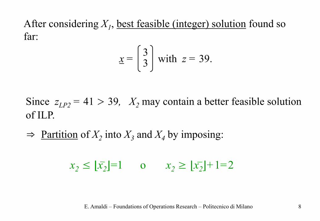
After considering X1, best feasible (integer) solution found so
far:
x = with z = 39. 3 3
Since zLP2 = 41 > 39, X2 may contain a better feasible solution
of ILP.
⇒ Partition of X2 into X3 and X4 by imposing:
x2 ≤ ⌊x2⌋=1 o x2 ≥ ⌊x2⌋+1=2
E. Amaldi – Foundations of Operations Research – Politecnico di Milano

9
z = 20
x2 = 2
x2 = 1 1
2
3
4
x2
1 2 3 4 5 6 x1
Subproblem S3
subregion X3
Subproblem S4 is infeasible (X4 = ø)
sol. x = with zLP3 = 365/9 40/9
1
E. Amaldi – Foundations of Operations Research – Politecnico di Milano

10
Branching tree:
LP
S1 S2
S3 S4
x1 ≥ 4 x1 ≤ 3
x2 ≤ 1 x2 ≥ 2
zLP2 = 41.25
zLP3 = 365/9 infeasible X4 = ø
z1LP = 39
integer sol.
Best feasible
solution found
so far
E. Amaldi – Foundations of Operations Research – Politecnico di Milano
11
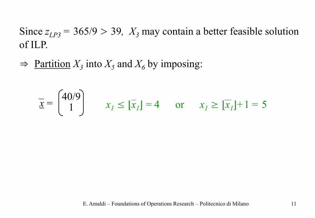
Since zLP3 = 365/9 > 39, X3 may contain a better feasible solution
of ILP.
⇒ Partition X3 into X5 and X6 by imposing:
x1 ≤ ⌊x1⌋ = 4 or x1 ≥ ⌊x1⌋+1 = 5 40/9
1 x =
E. Amaldi – Foundations of Operations Research – Politecnico di Milano
12
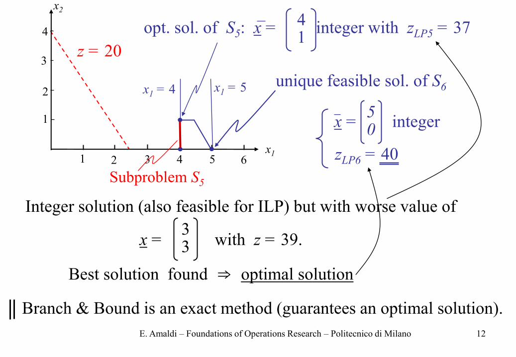
z = 20
Subproblem S5
opt. sol. of S5: x = integer with zLP5 = 37 4 1
1
2
3
4
x2
1 2 3 4 5 6 x1
x1 = 4 x1 = 5 unique feasible sol. of S6
5 0
x = integer
zLP6 = 40
Integer solution (also feasible for ILP) but with worse value of
x = with z = 39. 3 3
Best solution found ⇒ optimal solution
Branch & Bound is an exact method (guarantees an optimal solution).
E. Amaldi – Foundations of Operations Research – Politecnico di Milano
13
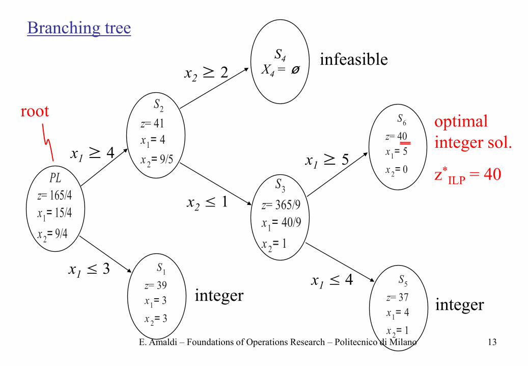
Branching tree
PL
z= 165/4
x1= 15/4
x 2= 9/4
S1
z= 39
x1= 3
x2= 3
S2
z= 41
x1= 4
x2= 9/5
S3
z= 365/9
x1= 40/9
x2= 1
S4
X4 = ø
S5
z= 37
x1= 4
x2= 1
S6
z= 40
x1= 5
x2= 0
root
integer integer
infeasible
x1 ≤ 3
x2 ≤ 1
x1 ≤ 4
x1 ≥ 4
x2 ≥ 2
x1 ≥ 5
optimal
integer sol.
z*ILP = 40
E. Amaldi – Foundations of Operations Research – Politecnico di Milano

14
The branching tree may not contain all possible nodes
(2d leaves)
A node of the tree has no child – is “fathomed”– if
• initial constraints + those on the arcs from the root are infeasible
(e.g. S4)
• optimal solution of the linear relaxation is integer (e.g. S1)
the value cTxLP of the optimal solution xLP of the linear
relaxation is worse than that of the best feasible (integer)
solution of ILP found so far. ≡ bounding criterion
E. Amaldi – Foundations of Operations Research – Politecnico di Milano

15
Observation: In the third case the feasible subregion of the
subproblem associated to that node cannot contain an integer
feasible solution that is better than the best feasible solution of
ILP found so far!
Bounding criterion often allows to “discard” a number of nodes
(subproblems).
E. Amaldi – Foundations of Operations Research – Politecnico di Milano

16
Choice of the node (subproblem) to examine:
• First deeper nodes (depth-first search strategy)
Simple recursive procedure, it is easy to reoptimize
but it may be costly in case of wrong choice.
• First more promising nodes (best-bound first strategy)
with the best value of linear relaxation
Typically generates a smaller number of nodes but suproblems are less constrained ⇒ takes longer to
find a first feasible solution and to improve it.
E. Amaldi – Foundations of Operations Research – Politecnico di Milano

17
Choice of the (fractional) variable for branching
It may turn out to be not the best choice to select the variable
xh whose fractional value is closer to 0,5 (hoping to obtain
two subproblems that are more stringent and balanced).
E. Amaldi – Foundations of Operations Research – Politecnico di Milano

No need to solve the linear relaxations of the ILP subproblems
from scratch with, for instance, the two-phase Simplex algorithm.
To efficiently find an optimal solution of the strengthened linear
relaxation with a new constraint, we can exploit the optimal
tableau of the previous linear relaxation and apply a single
iteration of the Dual simplex method (variant of the Simplex
method not covered here).
E. Amaldi – Foundations of Operations Research – Politecnico di Milano
Efficient solution of the linear relaxations
18

19
Branch & Bound is also applicable to mixed ILPs:
when branching just consider the fractional variables that must be
integer.
General method that can be adapted to tackle any discrete
optimization problem and many nonlinear optimization problems.
e.g., scheduling, traveling salesman problem,…
E. Amaldi – Foundations of Operations Research – Politecnico di Milano
Applicability of Branch and Bound approach

20
We “just” need
• Technique to partition a set of feasible solutions into two or more
subsets of feasible solutions (branch).
• Procedure to determine a bound on the cost of any solution in
such a subset of feasible solutions (bound).
E. Amaldi – Foundations of Operations Research – Politecnico di Milano
Observation: Branch-and-Bound can also be used as a heuristic by
imposing an upper bound on the computing time or on
the nmber of nodes that are examined.

21
5.1.2 B & B for a combinatorial optimization problem
Example: Scheduling problem on a single machine ( NP-hard )
Given n jobs with deadlines, and a single machine with processing
time for each job, determine a sequence that minimizes the total
delay.
n = 4 jobs processing
time
deadline
1 6 8
2 4 4
3 5 12
4 8 16
completed by
hour 8
in hours
E. Amaldi – Foundations of Operations Research – Politecnico di Milano

22
The sequence 1 – 2 – 3 – 4, has a total delay = 0 + 6 + 3 + 7 = 16.
Define xij =
Idea: partition the set of all feasible solutions based on the last job
that is processed.
Clearly x14 = 1 or x24 = 1 or x34 = 1 or x44 = 1
1 if job i is processed in j-th position
0 otherwise
hours
E. Amaldi – Foundations of Operations Research – Politecnico di Milano

23
D = total delay
If x44 = 1, job 4 is completed at the
end of hour 6 + 4 + 5 + 8 = 23,
namely with a delay of 23 – 16 = 7.
1 D ≥ 15
2 D ≥ 19
3 D ≥ 11
4 D ≥ 7
5 D ≥ 14
6 D ≥ 18
7 D ≥ 10
8 D = 12
9 D = 16
x14 = 1 x24 = 1
x44 = 1
x34 = 1
x13 = 1
x23 = 1
x33 = 1
x12 = 1 x22 = 1
⋮
Nodes with the smallest bound on D
are examined first.
Node 4; node 7; node 8;…
E. Amaldi – Foundations of Operations Research – Politecnico di Milano

24
For node 7: job 4 is the last one with a delay of 7 hours
job 3 is the next to last one with a delay of
6 + 4 + 5 – 12 = 3 hours
15 ⇒ D ≥ 7 + 3 = 10
Node 8: sequence 2 – 1 – 3 – 4 is a feasible solution with delay = 12
Observation: nodes 1, 2, 5 and 6 can be “pruned”!
E. Amaldi – Foundations of Operations Research – Politecnico di Milano

25
1 D ≥ 15
2 D ≥ 19
3 D ≥ 11
4 D ≥ 7
10 D ≥ 21
11 D ≥ 25
12 D ≥ 13
x14 = 1 x24 = 1
x44 = 1
x34 = 1
x13 = 1
x23 = 1
x43 = 1
⋮
11 + (6 + 4 + 8 – 16) = 13 11 + (6 + 4 + 8 – 8) = 21
job 1 next to last
⇒ Optimal sequence: 2 – 1 – 3 – 4 with D =12.
job 3 last
job 4 next to last
E. Amaldi – Foundations of Operations Research – Politecnico di Milano