5. Lecture SS 20005Cell Simulations1 V5: Functional inference from interaction networks.
39
5. Lecture SS 20005 Cell Simulations 1 V5: Functional inference from interaction networks
-
date post
19-Dec-2015 -
Category
Documents
-
view
217 -
download
0
Transcript of 5. Lecture SS 20005Cell Simulations1 V5: Functional inference from interaction networks.

5. Lecture SS 20005
Cell Simulations 1
V5: Functional inference from interaction networks

5. Lecture SS 20005
Cell Simulations 2
Aim: associated protein function at the proteomic scale
Even the best-studied model organisms contain a large number of proteins whose
functions are currently unknown. E.g. about one-third of the proteins in
Saccharomyces cerevisiae remain uncharacterized.
Traditionally, computational methods to assign protein function have relied largely
on sequence homology. The recent emergence of high-throughput experimental
datasets have led to a number of alternative, non-homology based methods for
functional annotation. These methods have generally exploited the concept of
guilt by association, where proteins are functionally linked through either
experimental or computational means.
Nabieva et al., Bioinformatics 21, i1 (2005)
5. Lecture SS 20005
Cell Simulations 3
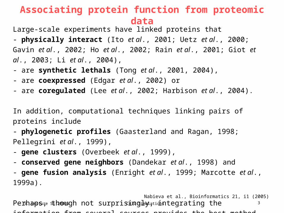
Associating protein function from proteomic data
Large-scale experiments have linked proteins that
- physically interact (Ito et al., 2001; Uetz et al., 2000; Gavin et al., 2002; Ho et
al., 2002; Rain et al., 2001; Giot et al., 2003; Li et al., 2004),
- are synthetic lethals (Tong et al., 2001, 2004),
- are coexpressed (Edgar et al., 2002) or
- are coregulated (Lee et al., 2002; Harbison et al., 2004).
In addition, computational techniques linking pairs of proteins include
- phylogenetic profiles (Gaasterland and Ragan, 1998; Pellegrini et al., 1999),
- gene clusters (Overbeek et al., 1999),
- conserved gene neighbors (Dandekar et al., 1998) and
- gene fusion analysis (Enright et al., 1999; Marcotte et al., 1999a).
Perhaps, though not surprisingly, integrating the information from several sources
provides the best method for linking proteins functionally.
Nabieva et al., Bioinformatics 21, i1 (2005)
5. Lecture SS 20005
Cell Simulations 4
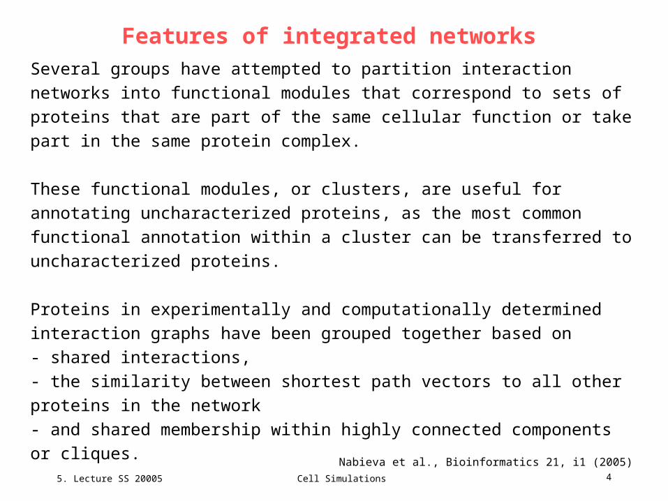
Features of integrated networks
Several groups have attempted to partition interaction networks into functional
modules that correspond to sets of proteins that are part of the same cellular
function or take part in the same protein complex.
These functional modules, or clusters, are useful for annotating uncharacterized
proteins, as the most common functional annotation within a cluster can be
transferred to uncharacterized proteins.
Proteins in experimentally and computationally determined interaction graphs
have been grouped together based on
- shared interactions,
- the similarity between shortest path vectors to all other proteins in the network
- and shared membership within highly connected components or cliques.
Nabieva et al., Bioinformatics 21, i1 (2005)

5. Lecture SS 20005
Cell Simulations 5
Features of integrated networks
Although such a simple majority vote approach, named Majority, has clear predictive value, it takes
only limited advantage of the underlying graph structure of the network. For example, in the interaction
network given in Figure 1, ‘Majority’ would assign functions to proteins d and f , but not to protein e, even
though our intuition might indicate that protein e has the same function as proteins d and f ; there are
several examples in the yeast proteome similar to this one (Schwikowski et al., 2000). Naturally, one
wishes to generalize this principle to consider functional linkages beyond the immediate neighbors in the
interaction graph, both to provide a systematic framework for analyzing the entirety of physical interaction
data for a given proteome and to make predictions for proteins with no annotated interaction partners.
Nabieva et al., Bioinformatics 21, i1 (2005)
The strategy described here is more closely related to recent attempts to classify proteins according to the functional annotations of their network neighbors; these methods do not explicitly cluster proteins. Schwikowski et al. (2000) use physical interaction data for baker’s yeast, and predict the biological process for each protein by considering its neighboring interactions and taking the three most frequent annotations.

5. Lecture SS 20005
Cell Simulations 6
Features of integrated networks
However, this approach, named Neighborhood, does not consider any aspect of
network topology within the local neighborhood.
E.g., Figure 2 shows two interaction networks that are treated equivalently when
considering a radius of 2 and annotating protein a; however, in the first case, there
is a single link that connects protein a to the annotated proteins, and in the second
case, there are several independent paths between a and the annotated proteins,
and moreover, two of these proteins are directly adjacent to a.
Nabieva et al., Bioinformatics 21, i1 (2005)
Hishigaki et al. (2001) extended Majority algorithm by predicting a protein’s function by looking at all proteins within a particular radius and finding over-represented functional annotations.

5. Lecture SS 20005
Cell Simulations 7
Method: physical interaction network
Construct the protein–protein physical interaction network using the protein
interaction dataset compiled by GRID (Breitkreutz et al., 2003).
The resulting network is a simple undirected graph G = (V , E), where there is a
vertex or node v V for each protein, and an edge between nodes u and
v if the corresponding proteins are known to interact physically (as determined by
one or more experiments).
Initially, we consider a graph with unit-weighted edges, and then consider
weighting the edges by our ‘confidence’ in the edge.
The weight of the edge between u and v is denoted by wu,v.
For all reported results, consider only the proteins making up the largest
connected component of the physical interaction map (4495 proteins and 12 531
physical interaction links).
Nabieva et al., Bioinformatics 21, i1 (2005)

5. Lecture SS 20005
Cell Simulations 8
Method: functional annotations
Several controlled vocabulary systems exist for describing biological function,
including Munich Information Center for Protein Sequences (MIPS) and the Gene
Ontology (GO) project.
We use the MIPS functional hierarchy, and consider the 72 MIPS biological
processes that comprise the second level of hierarchy.
Of the 4495 proteins in the largest connected component of the yeast physical
interaction map, 2946 have MIPS biological process annotations. We also
experimented with GO annotations; the overall conclusions made in this paper are
not affected.
Nabieva et al., Bioinformatics 21, i1 (2005)

5. Lecture SS 20005
Cell Simulations 9
Method: weighted functional linkages
The reliabilities of different data sources vary, even if they are based on the same
underlying technology.
In the context of network-based algorithms, it is possible to weight edges so as to model the
reliability of each interaction. For physical interactions, this reliability is in turn based on the
experimental sources that contribute to our knowledge
about the existence of the interaction.
To determine these values, separate all experimental sources of physical interaction data into
several groups, placing each high-throughput dataset into a separate group, and allocating
one group for the family of all specific experiments.
For each group of experiments, compute what fraction of its interactions connect proteins with
a known shared function. Assume that the reliabilities of different sources are independent,
and thus conclude by estimating the reliability of an interaction to be the noise (or unreliability)
of the underlying data sources.
If ri is the reliability of experimental group i, compute the reliability of the edge by 1 - i (1-ri ),
where the product runs over all experiments i where this interaction is found. This treats each
ri as a probability and assumes independence.
Nabieva et al., Bioinformatics 21, i1 (2005)

5. Lecture SS 20005
Cell Simulations 10
Algorithms: Majority
as in Schwikowsky et al. (2000): consider all neighboring proteins and sum up the
number of times each annotation occurs for each protein.
„The annotated functions of all neighbors of P are ordered in a list, from
the most frequent to the least frequent. Functions that occur the same number
of times are ordered arbitrarily. Everything after the third entry in the list
is discarded, and the remaining three or fewer functions are declared as
predictions for the function of P.“
In the case of weighted interaction graphs take a weighted sum.
Nabieva et al., Bioinformatics 21, i1 (2005)

5. Lecture SS 20005
Cell Simulations 11
Algorithms: Neighborhood algorithm
Adapted from Hishigaki et al. (2001) Protein interaction map (Figure B): each node represents a protein and each edge represents the interaction between two proteins.Predict function of each protein in the map (black circle in Figure C), based on the functions of ‘n-neighbouring proteins’, which are defined as a set of proteins reached via n physical interactions at most (n is an integer parameter).
E.g. all proteins enclosed by the inside dashed circle are ‘1-neighbouring proteins’, and those enclosed by the outside circle are ‘2-neighbouring proteins’. The protein of interest is assigned the function with the highest 2 value among functions of all n-neighbouring proteins. For each member of the function category, the 2 value is calculated using the following formula:
where i denotes a protein function, e.g. ‘Golgi’, ‘DNA repair’ and ‘transcription factor’, ei denotes an expectation number of i in n-neighbouring proteins expected from the distribution on the total map, and ni denotes an observed number of i in n-neighbouring proteins. Then, the function of a query protein is predicted to be the function i with the maximum 2 value. When there are multiple functions with the largest 2 value, both functions are assigned. The optimal n value is determined by a so-called self-consistency test, where the predicted functions of all proteins in the map are compared with their annotated functions for each n.
Here: consider neighborhoods of radius 1, 2 and 3.
This method does not extend naturally to the case of weighted interaction graphs.
Nabieva et al., Bioinformatics 21, i1 (2005)

5. Lecture SS 20005
Cell Simulations 12
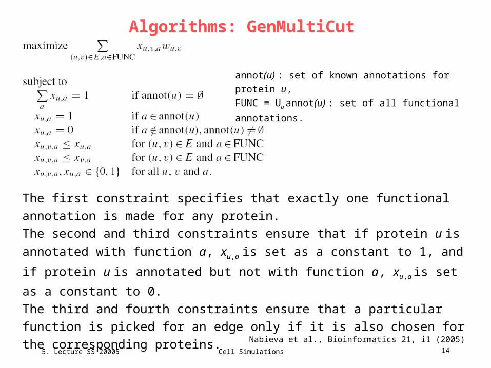
Algorithms: GenMultiCut
It was suggested that functional annotations on interaction networks should be
made in order to minimize the number of times different annotations are
associated with neighboring proteins.
Some authors used simulated annealing in an attempt to minimize this objective
function and aggregate results from multiple runs, whereas others used a
deterministic approximation, and consider the case where edges are weighted
using gene expression information.
The formulation in these two studies is similar to the minimum multiway k-cut
problem. In multiway k-cut, the task is to partition a graph in such a way that each
of k terminal nodes belongs to a different subset of the partition and so that the
(weighted) number of edges that are ‘cut’ in the process is minimized. In the more
general version of the multiway k-cut problem considered here, the goal is to
assign a unique function to all the unannotated nodes so as to minimize the sum
of the costs of the edges joining nodes with no function in common.
Nabieva et al., Bioinformatics 21, i1 (2005)

5. Lecture SS 20005
Cell Simulations 13
Algorithms: GenMultiCut
Although minimum multiway k-cut is NP-hard (Dahlhaus et al., 1994), it was
found that the particular instances of minimum multiway cut arising here can, in
practice, be solved exactly when stated as an ILP.
Introduce a node variable xu,a for each protein u and function a.
Set xu,a = 1 if protein u is predicted to have function a.
If a protein u has known functional annotations, variable xu,a is fixed as 1 for its
known annotations a and as 0 for all other annotations.
We also introduce an edge variable xu,v,a for each function a and each pair of
adjacent proteins u and v. This variable is set to 1 if both proteins u and v are
annotated with function a.
Minimizing the weighted number of neighboring proteins with different annotations
is the same as maximizing the number with the same annotation, and so we have
the following ILP:Nabieva et al., Bioinformatics 21, i1 (2005)
5. Lecture SS 20005
Cell Simulations 14
Algorithms: GenMultiCut
The first constraint specifies that exactly one functional annotation is made for any
protein.
The second and third constraints ensure that if protein u is annotated with function
a, xu,a is set as a constant to 1, and if protein u is annotated but not with function a,
xu,a is set as a constant to 0.
The third and fourth constraints ensure that a particular function is picked for an
edge only if it is also chosen for the corresponding proteins.
Nabieva et al., Bioinformatics 21, i1 (2005)
annot(u) : set of known annotations for protein u,
FUNC = Uu annot(u) : set of all functional annotations.

5. Lecture SS 20005
Cell Simulations 15
considering multiple GenMultiCut optimal solutions
An important consideration in this framework is the existence of multiple optimal
solutions. E.g. the network in Figure 3 has seven minimum cuts of value 1, and
while the GenMultiCut criterion does not favor any one cut over the
other, if we find all optimal cuts for this graph, we observe that x2 is in fact
annotated with F1 more often than with F2 in the assignments made by these cuts.
Thus, a sense of distance to annotated nodes is in fact present in the set of all
optimal solutions.
Nabieva et al., Bioinformatics 21, i1 (2005)

5. Lecture SS 20005
Cell Simulations 16
Algorithms: GenMultiCut
attempt to sample from the space of optimal solutions:
(1) add constraints to the ILP which require that each consecutive solution is
different from any previous solution in the value it assigns to at least 5% of the
node variables xu,a.
(2) introduce uniform self-weights wu,a for each protein u and function a.
These self-weights are then perturbed randomly by adding a very small offset to
each. Then maximize
a number of times
Nabieva et al., Bioinformatics 21, i1 (2005)

5. Lecture SS 20005
Cell Simulations 17
Algorithms: FunctionalFlow
The functional flow algorithm generalizes the principle of ‘guilt by association’ to groups of
proteins that may or may not interact with each other physically.
Treating each protein of known functional annotation as a ‘source’ of ‘functional flow’ for that
function. After simulating the spread over time of this functional flow through the
neighborhoods surrounding the sources, the ‘functional score’ is obtained for each protein in
the neighborhood; this score corresponds to the amount of ‘flow’ that the protein has
received for that function, over the course of the simulation.
The functional flow-based model allows us to incorporate a distance effect, i.e. the effect of
each annotated protein on any other protein depends on the distance separating these two
proteins.
Running this process for each biological function in turn, we obtain, for each protein, the
score for each function (the score may be 0 if the ‘flow’ for a function did not reach that
protein during the simulation). Thereupon, for any protein, we take the functions for which
the highest score was obtained as its predicted functions.
Nabieva et al., Bioinformatics 21, i1 (2005)

5. Lecture SS 20005
Cell Simulations 18
Algorithms: FunctionalFlow
More specifically, for each function in turn, we simulate the spread of functional flow by an
iterative algorithm using discrete time steps. We associate with each node (protein) a
‘reservoir’ which represents the amount of flow that the node can pass on to its neighbors at
the next iteration, and with each edge, a capacity constraint that dictates the amount of flow
that can pass through the edge during one iteration.
The capacity of an edge is taken to be its weight. Each iteration of the algorithm updates
the reservoirs using simple local rules: a node pushes the flow residing in its reservoir to its
neighbors proportionally to the capacities of the respective edges and subject to further
constraints that the amount of flow pushed through an edge during an iteration does not
exceed the capacity of the edge, and that flow only spreads ‘downhill’ (i.e. from proteins with
more filled reservoirs to nodes with less filled reservoirs).
Finally, at each iteration, an ‘infinite’ amount of flow is pumped into the source protein
nodes; thus, the sources always have enough flow in their reservoir to fill the capacity of
their outgoing edges.
Nabieva et al., Bioinformatics 21, i1 (2005)

5. Lecture SS 20005
Cell Simulations 19
Algorithms: FunctionalFlow
The functional score is the amount of flow that has entered a protein’s reservoir in
the course of all iterations. Since the flow is ‘pumped’ into the sources at each
step, the amount of flow a node receives from each source is greater for nodes
that are closer to that source than for nodes that are farther away from it.
Thus, a source’s immediate neighbor in the graph receives d iterationsworth of
flowfrom the source, whereas a node that is two links away from the source
receives d - 1 iterations worth of flow.
Similarly, the number of iterations for which the algorithm is run determines the
maximum shortest-path distance that can separate a recipient node from a source
in order for the flowto propagate from the source to the recipient. In the context of
protein interaction, a relatively small number of iterations is sufficient. We choose
d = 6, which is half the diameter of the yeast physical interaction network.
Nabieva et al., Bioinformatics 21, i1 (2005)
5. Lecture SS 20005
Cell Simulations 20
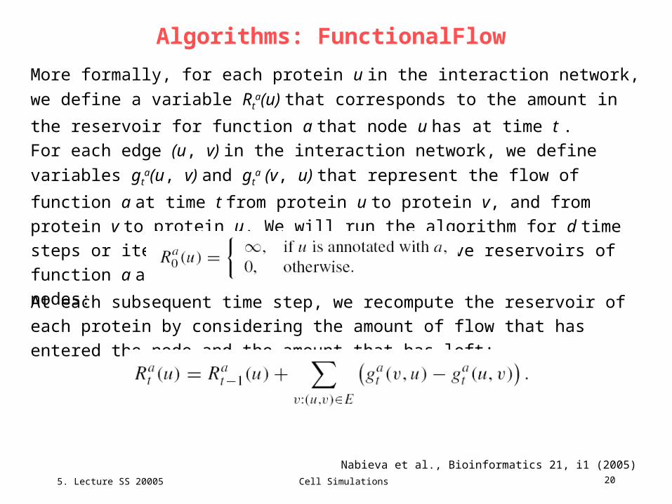
Algorithms: FunctionalFlow
More formally, for each protein u in the interaction network, we define a variable
Rta(u) that corresponds to the amount in the reservoir for function a that node u
has at time t .
For each edge (u, v) in the interaction network, we define variables gta(u, v) and gt
a
(v, u) that represent the flow of function a at time t from protein u to protein v, and
from protein v to protein u. We will run the algorithm for d time steps or iterations.
At time 0, we only have reservoirs of function a at annotated
nodes:
Nabieva et al., Bioinformatics 21, i1 (2005)
At each subsequent time step, we recompute the reservoir of each protein by
considering the amount of flow that has entered the node and the amount that has
left:

5. Lecture SS 20005
Cell Simulations 21
Algorithms: FunctionalFlow
Initially, at time 0, there is no flow on the edges, and ga
0 (u, v) = 0.
At each subsequent time step, we have the flow proceeding downhill and
satisfying the capacity constraints:
Nabieva et al., Bioinformatics 21, i1 (2005)
Finally, the functional score for node u and function a over d iterations is
calculated as the total amount of flow that has entered the node:
Why don‘t we simply take the current value of the reservoir?
5. Lecture SS 20005
Cell Simulations 22
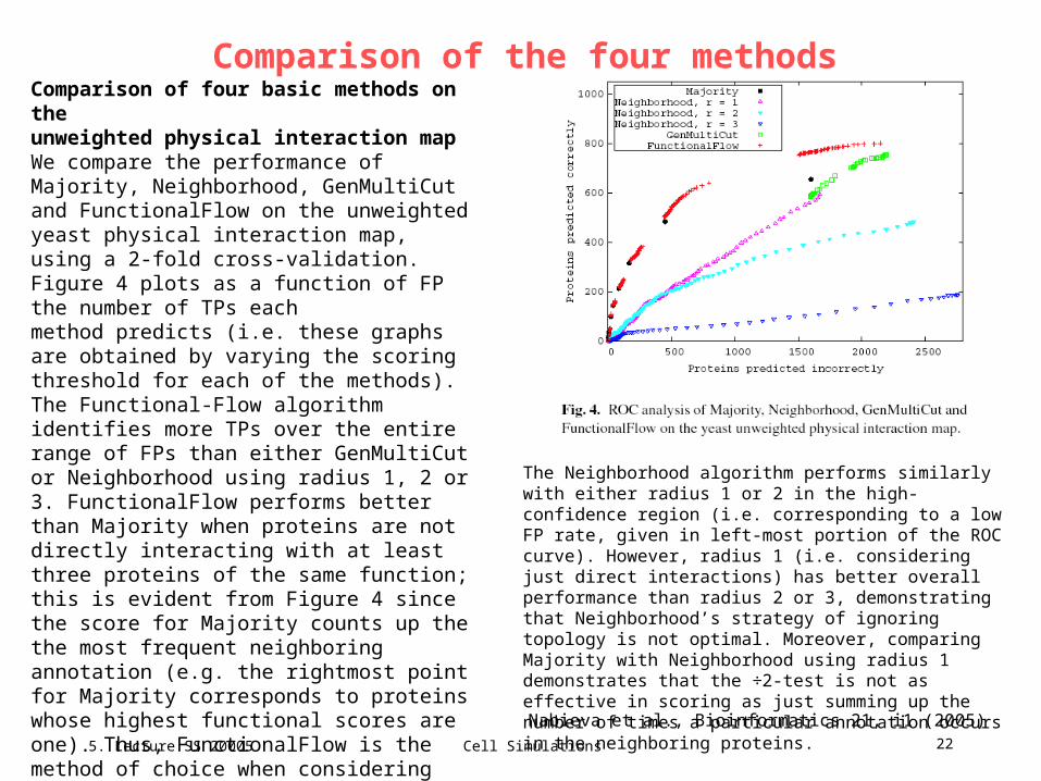
Comparison of the four methods
Comparison of four basic methods on theunweighted physical interaction mapWe compare the performance of Majority, Neighborhood, GenMultiCut and FunctionalFlow on the unweighted yeast physical interaction map, using a 2-fold cross-validation. Figure 4 plots as a function of FP the number of TPs eachmethod predicts (i.e. these graphs are obtained by varying the scoring threshold for each of the methods). The Functional-Flow algorithm identifies more TPs over the entire range of FPs than either GenMultiCut or Neighborhood using radius 1, 2 or 3. FunctionalFlow performs better than Majority when proteins are not directly interacting with at least three proteins of the same function; this is evident from Figure 4 since the score for Majority counts up the the most frequent neighboring annotation (e.g. the rightmost point for Majority corresponds to proteins whose highest functional scores are one). Thus, FunctionalFlow is the method of choice when considering proteins that do not interact with many annotated proteins. Even in well-characterized proteomes, such as baker’s yeast, there are ca. 1200 proteins that have fewer than three annotated neighbors.
Nabieva et al., Bioinformatics 21, i1 (2005)
The Neighborhood algorithm performs similarly with either radius 1 or 2 in the high-confidence region (i.e. corresponding to a low FP rate, given in left-most portion of the ROC curve). However, radius 1 (i.e. considering just direct interactions) has better overall performance than radius 2 or 3, demonstrating that Neighborhood’s strategy of ignoring topology is not optimal. Moreover, comparing Majority with Neighborhood using radius 1 demonstrates that the ÷2-test is not as effective in scoring as just summing up the number of times a particular annotation occurs in the neighboring proteins.

5. Lecture SS 20005
Cell Simulations 23
Reliability and data integration
To evaluate the approach for modeling physical interaction reliability as edge weights, we test
the performance of FunctionalFlow using three ways of assigning physical interaction
weights.
(1) assign each edge a unit weight; this corresponds to the unweighted physical interaction map.
(2) assign each experimental source a reliability score of 0.5; this rewards interactions that are
found by more than one experiment.
(3) assign each experimental source the predictive value (estimated in crossvalidation); here,
edges obtained from multiple, more reliable experiments are given higher weights.
Nabieva et al., Bioinformatics 21, i1 (2005)
Figure 5 shows that rewarding multiple experimental evidence is beneficial, but that the main advantage comes from taking into account the actual reliability values for the different experiments.

5. Lecture SS 20005
Cell Simulations 24
All methods perform better on weighted map
Figure 6 shows how Majority,
GenMultiCut and FunctionalFlow
perform on the yeast physical interaction
map, where edges are weighted by
individual experimental reliability.
The baseline performance of Majority
on the unweighted physical interaction
graph is also shown. There is substantial
improvement in predictions using all
three methods when incorporating edges
weighted by reliability.
Nabieva et al., Bioinformatics 21, i1 (2005)

5. Lecture SS 20005
Cell Simulations 25
Is it useful to provide more information?
We further explored whether the
network analysis algorithms would
perform well when other types of
experimental information are added.
As a proof of principle, we explore the
effect of adding genetic linkages to
the graph (synthetic lethals).
As is evident from the figure, adding
genetic interaction data significantly
improves prediction quality.
Nabieva et al., Bioinformatics 21, i1 (2005)

5. Lecture SS 20005
Cell Simulations 26
Conclusions
Network analysis algorithm FunctionalFlow provides an effective means for
predicting protein function from protein interaction maps.
The algorithm utilizes indirect network interactions, network topology, network
distances and edges weighted by reliability estimated from multiple data sources.
The simplest methods, such as Majority, perform well if there are enough direct
neighbors with known function.
Simple independence assumptions were made for estimating the reliability of
interactions. Although these work reasonably well, it may be even more beneficial
to use a more sophisticated approach for weight assignment and perform more
complete data integration.
Finally, although the method was applied to baker’s yeast, FunctionalFlow is
likely to be especially useful when analyzing largely uncharacterized proteomes
where computational methods are used to infer protein interaction maps.
Nabieva et al., Bioinformatics 21, i1 (2005)

5. Lecture SS 20005
Cell Simulations 27
Alternative scheme to combine information from various source: Bayesian network
Knowing the correct overall structures of gene networks will be invaluable for characterizing
the complex roles of individual genes and the interplay between the many systems in a cell.
Deriving gene networks from heterogeneous functional genomics data is often difficult,
because experiments such as microarray analyses of gene expression or systematic protein
interaction mapping measure different aspects of gene or protein associations. E.g.
Affinity purification of proteins analyzed by MS: measures the tendency for proteins to be
components of the same physical complex, although not necessarily to contact each other
directly.
Yeast two-hybrid assays: often indicate direct physical interactions (stable or transient)
between proteins.
Synthetic lethal screens: measure the tendency for genes to compensate for the loss of
other genes.
These analyses range considerably in accuracy, and it is not clear a priori which
measurements are correct.
In spite of these differences, these data sets can, in principle, be computationally integrated,
primarily by the reconstruction of network models of the relations between genes.
Lee, ..., Marcotte, Science 306, 1555 (2004)
5. Lecture SS 20005
Cell Simulations 28
Aim: construct complete network of gene association
Network reconstructions have largely focused on physical protein interaction and so
represent only a subset of biologically important relations.
Aim: construct a more accurate and extensive gene network by considering functional,
rather than physical, associations, realizing that each experiment, whether genetic,
biochemical, or computational, adds evidence linking pairs of genes, with associated error
rates and degree of coverage.
In this framework, gene-gene linkages are probabilistic summaries representing functional
coupling between genes. Only some of the links represent direct protein-protein interactions;
the rest are associations not mediated by physical contact, such as regulatory, genetic, or
metabolic coupling, that, nonetheless, represent functional constraints satisfied by the cell
during the course of the experiments.
Working with probabilistic functional linkages allows many diverse classes of
experiments to be integrated into a single coherent network which enables the linkages
themselves to be more reliably
Lee, ..., Marcotte, Science 306, 1555 (2004)
5. Lecture SS 20005
Cell Simulations 29
Method for integrating functional genomics data
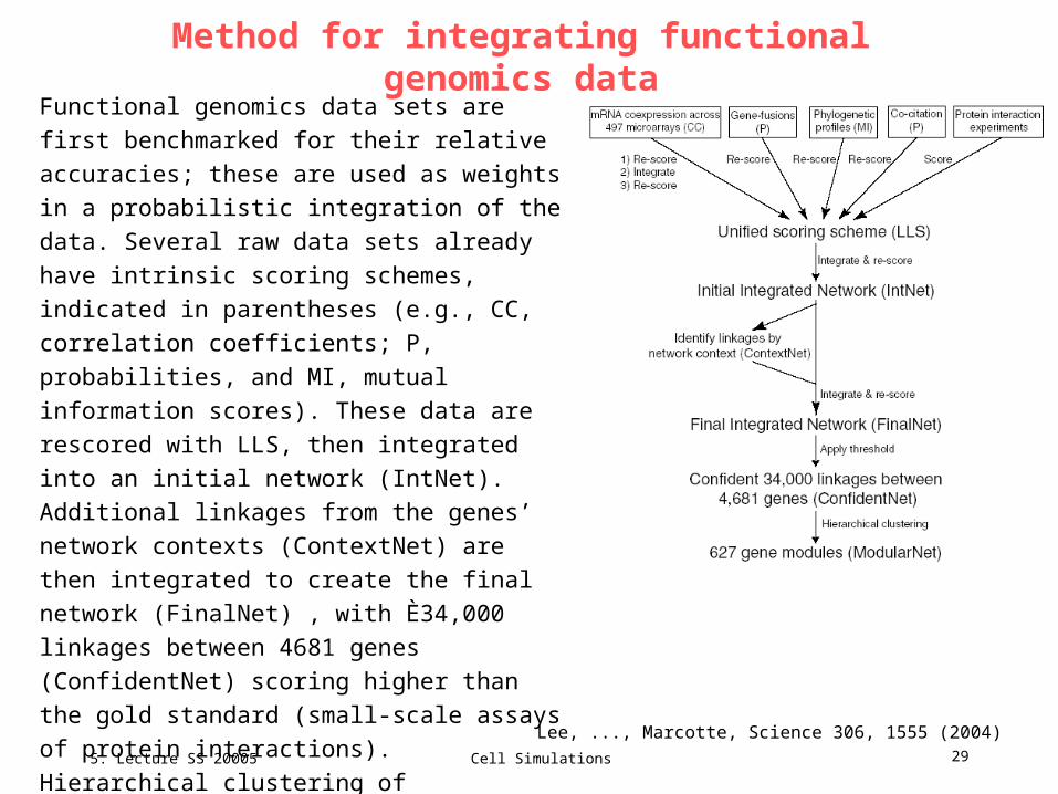
Functional genomics data sets are first
benchmarked for their relative accuracies; these
are used as weights in a probabilistic integration of
the data. Several raw data sets already have
intrinsic scoring schemes, indicated in
parentheses (e.g., CC, correlation coefficients; P,
probabilities, and MI, mutual information scores).
These data are rescored with LLS, then integrated
into an initial network (IntNet). Additional linkages
from the genes’ network contexts (ContextNet) are
then integrated to create the final network
(FinalNet) , with È34,000 linkages between 4681
genes (ConfidentNet) scoring higher than the gold
standard (small-scale assays of protein
interactions). Hierarchical clustering of
ConfidentNet defined 627 modules of functionally
linked genes spanning 3285 genes
(‘‘ModularNet’’), approximating the set of cellular
systems in yeast.Lee, ..., Marcotte, Science 306, 1555 (2004)
5. Lecture SS 20005
Cell Simulations 30
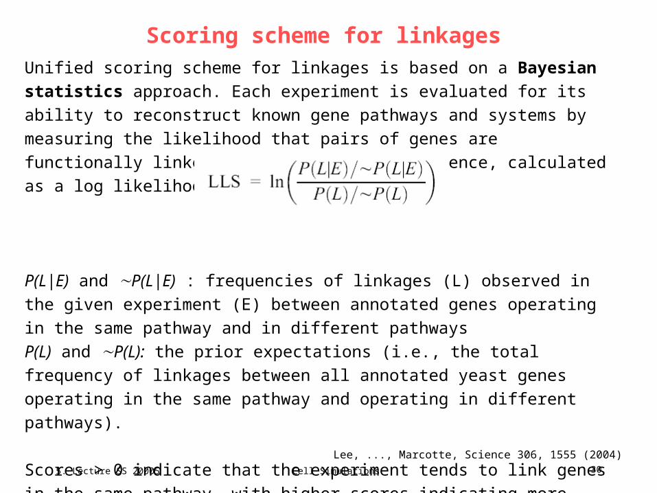
Scoring scheme for linkages
Unified scoring scheme for linkages is based on a Bayesian statistics approach.
Each experiment is evaluated for its ability to reconstruct known gene pathways
and systems by measuring the likelihood that pairs of genes are functionally
linked conditioned on the evidence, calculated as a log likelihood score:
P(L|E) and P(L|E) : frequencies of linkages (L) observed in the given
experiment (E) between annotated genes operating in the same pathway and in
different pathways
P(L) and P(L): the prior expectations (i.e., the total frequency of linkages
between all annotated yeast genes operating in the same pathway and operating
in different pathways).
Scores > 0 indicate that the experiment tends to link genes in the same pathway,
with higher scores indicating more confident linkages.
Lee, ..., Marcotte, Science 306, 1555 (2004)

5. Lecture SS 20005
Cell Simulations 31
Benchmarks
As scoring benchmarks, the method was tested against two primary annotation
references: the Kyoto-based KEGG pathway database and the experimentally
observed yeast protein subcellular locations determined by genome-wide green
fluorescent protein (GFP)–tagging and microscopy.
KEGG scores were used for integrating linkages, with the other benchmark
withheld as an independent test of linkage accuracy.
Cross-validated benchmarks and benchmarks based on the Gene Ontology (GO)
and KOG gene annotations provided comparable results.
Lee, ..., Marcotte, Science 306, 1555 (2004)

5. Lecture SS 20005
Cell Simulations 32
Functional inference from interaction networks
Benchmarked accuracy and extent of functional genomics data sets and the integrated networks. A critical point is the comparable performance of the networks on distinct benchmarks, which assess the tendencies for linked genes to share (A) KEGG pathway annotations or (B) protein subcellular locations. Each x axis indicates the percentage of protein-encoding yeast genes provided with linkages by the plotted data; each y axis indicates relative accuracy, measured as the of the linked genes’ annotations on that benchmark. The gold standards of accuracy (red star) for calibrating the benchmarks are smallscale protein-protein interaction data from DIP. Colored markers indicate experimental linkages; gray markers, computational. The initial integrated network (lower black line), trained using only the KEGG benchmark, has measurably higher accuracy than any individual data set on the subcellular localization benchmark; adding context-inferred linkages in the final network (upper black line) further improves the size and accuracy of the network.
Lee, ..., Marcotte, Science 306, 1555 (2004)

5. Lecture SS 20005
Cell Simulations 33
Features of integrated networks
Functional linkages were first inferred on the basis of genes‘ mRNA coexpression across each of 12 sets of DNA microarray experiments (497 microarray experiments in total), then integrated via a rank-weighted sum of log likelihood scores to create the combined set of coexpression-derived linkages. To construct the initial integrated network (BIntNet,[ Fig. 1), we combined 8 categories of data, including the physical and genetic interaction data sets, mRNA coexpression linkages, functional linkages from literature mining, and computational linkages from two comparative genomics methods, Rosetta stone (gene-fusion) linkages and phylogenetic profiles.
Lee, ..., Marcotte, Science 306, 1555 (2004)
Integrating functional genomics data also allowed discovery of additional relations between genes linked, in turn, to a common set of genes [BContextNet]; these linkages were scored and integrated as above to construct the final gene network (BFinalNet, see figure). The final network has 34,000 linkages at an accuracy comparable to the gold standard small-scale interaction assays, which provides linkages (BConfidentNet) for more than 4681 yeast genes (81% of the yeast proteome). The network is reasonably distinct from networks of physical interacting proteins Ee.g., sharing only È16% of linkages with (Jansen et al.).
The final network shows extensive clustering of genes into modules, evident in the ‘‘clumping’’ (A).
5. Lecture SS 20005
Cell Simulations 34
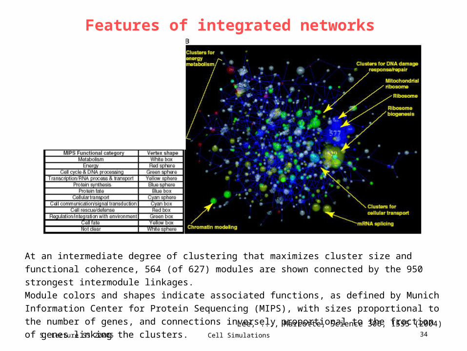
Features of integrated networks
At an intermediate degree of clustering that maximizes cluster size and functional coherence, 564 (of
627) modules are shown connected by the 950 strongest intermodule linkages.
Module colors and shapes indicate associated functions, as defined by Munich Information Center for
Protein Sequencing (MIPS), with sizes proportional to the number of genes, and connections inversely
proportional to the fraction of genes linking the clusters.
Lee, ..., Marcotte, Science 306, 1555 (2004)

5. Lecture SS 20005
Cell Simulations 35
Features of integrated networks
Adding context-inferred linkages increased clustering of genes, which produced a
highly modular gene network with well-defined subnetworks.
We expected these gene clusters to reflect gene systems and modules. We could
therefore generate a simplified view of the major trends in the network (Fig. 3B) by
clustering genes of ConfidentNet according to their connectivities. Of the 4681
genes, 3285 (70.2%) were grouped into 627 clusters, reflecting the high degree of
modularity.
Genes‘ functions within each cluster are highly coherent, and with 2 to 154 genes
per cluster (ca. 5 genes per cluster on average), the clusters effectively capture
typical gene pathways and/or systems.
Lee, ..., Marcotte, Science 306, 1555 (2004)
5. Lecture SS 20005
Cell Simulations 36
Features of integrated networks
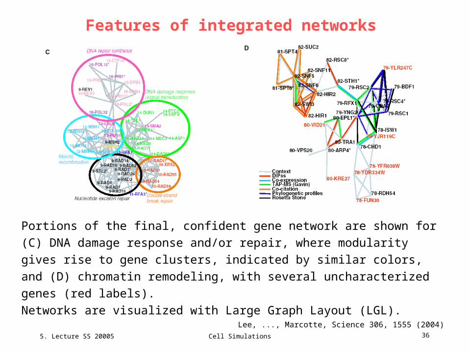
Portions of the final, confident gene network are shown for (C) DNA damage
response and/or repair, where modularity gives rise to gene clusters, indicated by
similar colors, and (D) chromatin remodeling, with several uncharacterized
genes (red labels).
Networks are visualized with Large Graph Layout (LGL).
Lee, ..., Marcotte, Science 306, 1555 (2004)

5. Lecture SS 20005
Cell Simulations 37
Features of integrated networks
A region of the modular network centered on the DNA damage response and
repair systems is shown in Fig. 3C. The network is clearly hierarchical: Individual clusters
represent distinct systems related to DNA damage response and/or repair; these clusters
are in turn connected to modules of cell cycle regulatory genes and chromatin silencing,
functionally linked to the DNA damage response and/or repair system.
One can infer individual genes‘ functions on the basis of linked neighbors. (Comment: this simple scheme can be improved by combining approach with Nabieva et al.)
For example, seven uncharacterized genes are implicated in chromatin remodeling (Fig.
3D). All but 1 of the 18 linkages made by these genes arise from the comparative genomics
analysis or from the network context methods, which represent examples of the insights that
arise only after data integration. Three of the uncharacterized proteins are predicted by
sequence homology to have helicase activity, which is reasonable for a relation to chromatin
remodeling; four of these proteins localize to the nucleus, further supporting their
association. After this network‘s construction, one gene, VID21, was implicated in chromatin
modification as a component of the NuA4 histone acetyl transferase.
Lee, ..., Marcotte, Science 306, 1555 (2004)

5. Lecture SS 20005
Cell Simulations 38
Experimental verification of one prediction
The function of the RNA helicase PRP43, previously thought to be involved only in
pre-mRNA splicing and implicated in lariatintron release from the spliceosome, is
also clarified in the network.
PRP43 is linked most strongly to genes of ribosome biogenesis and rRNA
processing. The tightest links are to ERB1, RRB1, NUG1, LHP1, and PWP1, the
first three of which are confirmed ribosome biogenesis factors. These links derive
only from the coexpression and context methods; data integration is therefore
critical.
The association of PRP43 with ribosome biogenesis has now been experimentally
validated: the growth defect conferred by a PRP43 conditional lethal mutation
corresponds to a rapid and major defect in rRNA processing.
These data indicate that rRNA processing is the essential function of PRP43, and
it joins a growing group of RNA helicases with two or more distinct functions.
Lee, ..., Marcotte, Science 306, 1555 (2004)

5. Lecture SS 20005
Cell Simulations 39
Summary
The probabilistic gene network integrates evidence from diverse sources to reconstruct an
accurate network, by estimating the functional coupling among yeast genes, and provides a
view of the relations between yeast proteins distinct from their physical interactions.
The application of this strategy to other organisms, such as to the human genome, is
conceptually straightforward:
(i) assemble benchmarks for measuring the accuracy of linkages between human genes
based on properties shared among genes in the same systems,
(ii) assemble gold standard sets of highly accurate interactions for calibrating the
benchmarks, and
(iii) benchmark functional genomics data for their ability to correctly link human genes, then
integrate the data as described.
New data can be incorporated in a simple manner serving to reinforce the correct linkages.
Thus, the gene network will ultimately converge by successive approximation to the
correct structure simply by continued addition of functional genomics data in this
framework.
Lee, ..., Marcotte, Science 306, 1555 (2004)