5 Greek Part Patras - BOKU · precipitation considers cyclonic/ anticyclonic conditions as well as...

5 Greek Part Patras

5.1 Table of contents (Greek group from Patras) 5.1 Table of contents (Greek group from Patras) ................................................................. 5-3 5.2 Study area ....................................................................................................................... 5-4 5.3 Methodology................................................................................................................... 5-4

5.3.1 Downscaling – classification and related models................................................... 5-4 5.3.1.1 Downscaling from Principal Component Analysis (PCA) and k-mean clustering CP-type classification (WCS1)....................................................................................... 5-4 5.3.1.2 Downscaling from wind direction CP-type classification (WCS2).................... 5-4 5.3.1.3 Downscaling from CP-type classification based on wind direction and cyclonic/anticyclonic conditions (WCS3) ...................................................................... 5-5 5.3.1.4 Downscaling from CP-type classification based on a reduced number of wind directions and cyclonic/anticyclonic conditions (WCS4) .............................................. 5-6 5.3.1.5 Objective indices of quality for the downscaling approach ............................... 5-7 5.3.1.6 Models ................................................................................................................ 5-7

5.4 Calibration and validation .............................................................................................. 5-8 5.4.1 Large scale pressure distribution fields .................................................................. 5-8 5.4.2 Calibration of the downscaling approach ............................................................. 5-10

5.4.2.1 Temperature and precipitation at the basin scale.............................................. 5-10 5.4.2.2 Hydrology at the basin scale............................................................................. 5-13 5.4.2.3 Possible reasons of temperature and precipitation changes in case of increased CO2-concentration........................................................................................................ 5-15 5.4.2.4 Validation of the downscaling approach .......................................................... 5-25

5.4.3 Calibration of the hydrological model.................................................................. 5-31 5.4.3.1 Quantification of the model error ..................................................................... 5-31 5.4.3.2 Calibration of ENNS-model ............................................................................. 5-31 5.4.3.3 Calibration of ARNO-model ............................................................................ 5-34

5.5 Impact studies (2*CO2)................................................................................................ 5-42 5.5.1 ........Changes in geopotential height and in the occurrence probabilities of the weather types.................................................................................................................................. 5-42 5.5.2 Hydrometeorological impact of climate change on basin ........................................42

5.5.2.1 Changes in the cumulative probability of temperature.........................................42 5.5.2.2 Changes in the cumulative probability of precipitation........................................42

5.5.3 Impact on basin hydrology .......................................................................................43 5.5.4 Uncertainties in the results .......................................................................................49

5.2 Study area The description of the Mesochora basin can be found in chapter 4.2.

5.3 Methodology

5.3.1 Downscaling – classification and related models

5.3.1.1 Downscaling from Principal Component Analysis (PCA) and k-mean clustering CP-type classification (WCS1)

Principal Component Analysis (PCA) combined with k-mean clustering (Matyasovszky et al., 1994) have been used to define ten weather types for both winter (October to March) and summer (April to September), valid for whole Europe. This classification scheme is characterised in the following as WCS1). The classification of the historic pressure distribution fields as well as of GCM output for the 1*CO2 and 2*CO2 scenario, is based on the 700hPa isobar. The circulation pattern characteristics for each weather type are described in Hebenstreit (1995).

5.3.1.2 Downscaling from wind direction CP-type classification (WCS2) For the estimation of wind directions geopotential height corresponding to 500hPa isobar at six grid points around the Mesohora basin with coordinates given in Table 5.3.1 have been used. From the geopotential height, geopotential height gradients have been estimated.

Tab. 5.3.1: Coordinates of grid points used for wind direction estimation

POINT LATITUDE LONGITUDE 1 37.50 20.00 2 37.50 22.50 3 40.00 20.00 4 40.00 22.50 5 42.50 20.00 6 42.50 22.50

By four triplets of these points, four triangles are formed and the geopotential height values are taken as heights on each of the triangle's apex. Gradients result as the pressure difference between two points over their distance, which is taken as unit length. The gradient directions are classified in eight 45-degree angles, and is given an identifier D1, D2,...,D8 starting from East and proceeding counter-clockwise (Fig. 5.3.1). With this procedure a daily time series of geopotential height gradients and geopotential height gradient directions is produced. For the elevation of 500hPa isobar, geopotential height gradient is related to wind direction. Wind direction is perpendicular to gradient in such a way that in the wind direction the low-pressure field is on the left and the high on the right side.

0° [East]

D2

45°

90° [North]

135

D1

D3

D4

Fig. 5.3.1: Directions of geopotential height used in classification scheme WCS2

5.3.1.3 Downscaling from CP-type classification based on wind direction and cyclonic/anticyclonic conditions (WCS3)

According to Maheras and Patrikas (1998, personal communication) an improvement of the classification scheme WCS2 could result if in addition to wind direction in a definite day the kind of the prevailing atmospheric system (cyclone or anticyclone) is taken into consideration. Conditions in a day are here considered to be cyclonic/ anticyclonic, if the geopotential height in this day is smaller/larger than the corresponding long term monthly mean of the geopotential height. This results to a classification scheme with 16 weather types, eight for cyclonic and eight for anticyclonic conditions. However, the increased number of weather types reduces the number of rainy days corresponding to each of them, which causes problems to the downscaling procedure. For this reason the number of weather types has been reduced grouping together those corresponding to directions D5 to D8 have low occurrence probability. Thus, classification scheme WCS3 is characterised by ten weather types, which are related to the geopotential height gradient as shows Table 5.3.2.

180° [West]

225°

270° [South]

D5

D6 D7

D8

Tab. 5.3.2: Geopotential height gradient direction for the weather types of classification scheme WCS3

WEATHER TYPE

DIRECTION OF GEOPOTENTIAL HEIGHTGRADIENT

1* D1 2 D2 3 D3 4 D4 5 D5,D6,D7,D8 6** D1 7 D2 8 D3 9 D4 10 D5,D6,D7,D8

* Weather types 1-5 correspond to cyclonic conditions ** Weather types 6-10 correspond to anticyclonic conditions

5.3.1.4 Downscaling from CP-type classification based on a reduced number of wind directions and cyclonic/anticyclonic conditions (WCS4)

Given the problems resulting in downscaling due to large number of weather types, a further classification has been used. It is characterised by a smaller number of weather types and uses different weather types for downscaling temperature and precipitation. The classification scheme used for downscaling temperature distinguishes between two weather types, the first one for cyclonic and the second one for anticyclonic conditions. Cyclonic and anticyclonic conditions are defined as described previously. The classification scheme for downscaling precipitation considers cyclonic/ anticyclonic conditions as well as two wind directions, the first one including south, south east and south west winds and the second one including north, north east and north west winds. Owing to the fact that wind direction is perpendicular to geopotential height gradient, the aforementioned two wind directions are related to geopotential height gradient directions as it is shown in Table 5.3.3, which summarises the definition of WCS4.

Tab. 5.3.3: Definition of classification scheme WCS4

WEATHER TYPE

GRADIENT DIRECTION

CYCLONIC COND.

ANTICYCL. COND.

DOWNSCALING OF

1 2

- -

+ -

- +

temperature temperature

1 2 3 4

D3, D4, D5, D6 D1, D2, D7, D8 D3, D4, D5, D6 D1, D2, D7, D8

+ + - -

- - + +

precipitation precipitation precipitation precipitation

5.3.1.5 Objective indices of quality for the downscaling approach In Table 5.3.4 the values of the performance indices for downscaling of precipitation (see definition of these indices in the contribution of the German group) are given. For the estimation the mean basin precipitation has been used, which is calculated taking into consideration the orography of the basin (see Annex of Second Annual Report). Classification schemes WCS3 and WCS4 appear the largest values of all performance indices, which indicates that these are the most appropriate for the Mesohora basin. However, it is difficult to decide which of them is the most appropriate because, as it can be seen directly from the definition of the indices I1 and I2, their values increase when the rainy days are concentrated in less weather types. Thus, although performance indices are higher for WCS4 it can not be said that it is a better classification scheme than WCS3. Therefore both schemes have been applied in the downscaling procedure. Tab. 5.3.4: Values of performance indices for the classification schemes

WCS1 WCS2 average W+S Winter Summer average W+S Winter Summer

I1 I2 I3 KI

0.098 2.343 0.361 0.016

0.164 4.002 0.502 0.031

0.032 0.683 0.220 0.0014

0.118 2.762 0.555 0.0248

0.158 4.190 0.681 0.040

0.078 1.334 0.429 0.0095

WCS3 WCS4 average W+S Winter Summer average W+S winter Summer

I1 I2 I3 KI

0.184 3.795 0.762 0.063

0.221 5.459 0.759 0.086

0.146 2.131 0.765 0.039

1.191 3.953 0.787 0.071

0.239 5.945 0.831 0.111

0.143 1.960 0.744 0.030

5.3.1.6 Models For space-time modeling of temperature and precipitation conditioned on weather types the models developed by Matyasovszky et al. (1994) have been used. A short description of the model is given also by the Austrian group in the Annex of the first annual report. For rainfall - runoff simulation in Mesohora basin the ENNS model developed by the Austrian group (Nachtnebel et al., 1993) as well as the ARNO model developed by the Italian group (Todini, 1996) have been used. The models are described in the contributions of these groups.

5.4 Calibration and validation

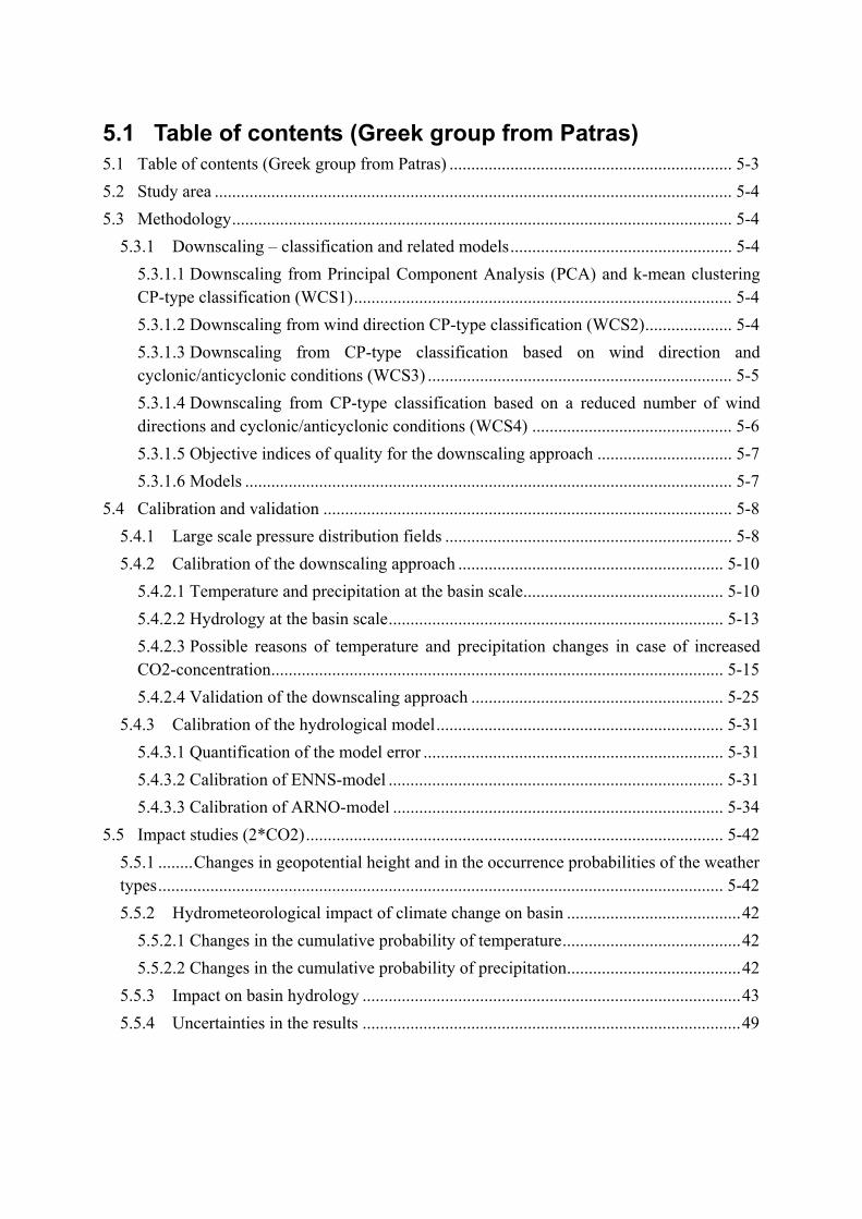
5.4.1 Large scale pressure distribution fields The historical data of pressure distribution fields used in this study have been provided by the National Center for Atmospheric Research (NCAR) in USA. They contain the geopotential height of 500hPa and 700hPa pressure level. Geopotential heights for the CO2-scenarios (1*CO2 and 2*CO2) have been taken from the results of General Circulation Model ECHAM-3 T42 of Max Plank Institute in Germany. In Fig. 5.4.1 the spatial mean of geopotential height for the period 1972-1992 estimated from the values at the grid points given in Table 5.3.1, is compared with the GCM results for the scenario 2*CO2 and a period of twenty years. Geopotential height in 2*CO2 case is slightly increased compared to historic case (see also Table 5.4.1). However, from Fig. 5.4.2 it can be concluded that GCM values are probably overestimated. In this figure mean values of geopotential height for the weather types corresponding to classification scheme WCS3 are given for the historic, the 1*CO2 and 2*CO2 case. It can be seen that the differences between historic case and 1*CO2 are larger than the differences between 1*CO2 and 2*CO2. The fact that 1*CO2 should be closer to historic case than to 2*CO2 indicates that the geopotential height values of the aforementioned GCM are overestimated. Thus, the actual differences between historic data and 2*CO2 cases are probably smaller than those given in Table 5.4.1. Tab. 5.4.1: Comparison of spatially mean of geopotential height for 500hPa pressure level for a period of 20 years

GEOPOTENTIAL HEIGHT WINTER (MEAN FOR 20 YEARS)

GEOPOTENTIAL HEIGHT SUMMER (MEAN FOR 20 YEARS)

historic 5602.78m 5741.94m 2*CO2 5702.26m 5793.78m increase 1.8% 0.9%

-500 0 500 1000 1500 2000 2500 3000 3500 4000

52005300540055005600570058005900600061006200

winter half year historic '72-'92 2xCO2

geop

oten

tial h

eigh

t

time in days

( a )

-500 0 500 1000 1500 2000 2500 3000 3500 4000

540055005600570058005900600061006200

summer half year historic '72-'92 2xCO2

geop

oten

tial h

eigh

t

time in days

Fig. 5.4.1: Change of geopotential height for the 500hPa isobar, due to CO2 increase: a) winter half year b) summer half year

1 2 3 4 5 6 7 8 9 105500

5550

5600

5650

5700

5750

5800

winter half year

spat

ially

ave

rage

d ge

opot

entia

l he

ight

in m

for 5

00hP

a

Weather type

historical '72-'92 1xCO2 2xCO2

( b )

( a )

1 2 3 4 5 6 7 8 9 105600

5650

5700

5750

5800

5850

5900summer half year

spat

ially

ave

rage

d ge

opot

entia

l

heig

ht in

m fo

r 500

hPa

Weather type

historical '72-'92 1xCO2 2xCO2

Fig. 5.4.2: Spatially averaged geopotential height (500 hPa) for different weather types: a) winter half year b) summer half year

5.4.2 Calibration of the downscaling approach

5.4.2.1 Temperature and precipitation at the basin scale The hydrological data (temperature and precipitation) for the Mesohora basin used in this study have been provided by Dr. D. Panagoulia in the frame of a cooperation with the group of University of Thessaloniki. Precipitation data (daily values) are available for nine stations in and around the Mesohora basin. The position of the precipitation stations is shown in Fig. 5.4.3. For temperature, data from the station Vakari have been used. Mean daily temperatures have been calculated as the mean of minimal and maximal temperature of a day. Temperatures in elevation zones different from the elevation of Vakari, which are required for hydrological modeling, are estimated using a lapse rate of 0.70C/100m. Fig. 5.4.4 shows the annual mean temperature. The trend of temperature is statistically not significant. Fig. 5.4.5 shows

( b )

6 4 08 0 09 6 0

1 1 2 01 2 8 01 4 4 01 7 6 01 9 2 02 0 8 02 2 4 02 4 0 0

Altitude [m]

N

Paleochori

Matsouk

Pahtouri

Katafyto

Pertouli

Vakari

Tyrna

Vathyrema

Stournareika

Fig. 5.4.3: Digital terrain model of the Mesohora basin with locations of stations the long term mean monthly temperature. The lowest values appear in December, January and February and the highest in June, July and August. In Table 5.4.2 the correlation matrix of the precipitation stations for lag=0 is given. The strongest correlation exists between the stations Vakari and Vathirema. Both of them are also well correlated to four other stations (correlation coefficients > 0.7). Between the other stations the correlation is not significant, probably due to local processes resulting from the orography, which in Mesohora basin is, as Fig. 5.4.3 shows, complicated. The lag 1 correlation of the precipitation stations (Table 5.4.3) is considerably reduced. Fig. 5.4.6(a) shows the annual precipitation height in the investigated period for five stations. Precipitation height varies considerably in the basin. The stations show different trends. Katafyto Pertouli and Vakari show an increasing trend in the investigated period whereas Pahtouri and Matsouki a decreasing trend. Fig. 5.4.6(b) shows the distribution over the year of the basin mean precipitation. The main precipitation amount is concentrated in the period from October to February. Tab. 5.4.2: Correlation matrix (lag=0) for the precipitation stations in Mesohora basin. (KAT=Katafyto, MAT=Matsouki, PAH=Pahtouri, PAL=Paleohori, PER=Pertouli, STO=Stournareika, TYR=Tyrna, VAK=Vakari, VAT=Vathyrema)

KAT MAT PAH PAL PER STO TYR VAK VAT KAT 1 0,526 0,552 0,437 0,458 0,543 0,351 0,543 0,633 MAT 0,526 1 0,762 0,635 0,659 0,568 0,487 0,785 0,753 PAL 0,552 0,762 1 0,583 0,618 0,611 0,464 0,781 0,725 PAH 0,437 0,635 0,583 1 0,689 0,540 0,660 0,660 0,687 PER 0,458 0,659 0,618 0,689 1 0,576 0,665 0,730 0,697 STO 0,543 0,568 0,611 0,540 0,576 1 0,504 0,640 0,780 TYR 0,351 0,487 0,464 0,660 0,665 0,504 1 0,551 0,600 VAK 0,543 0,785 0,781 0,660 0,730 0,640 0,551 1 0,816

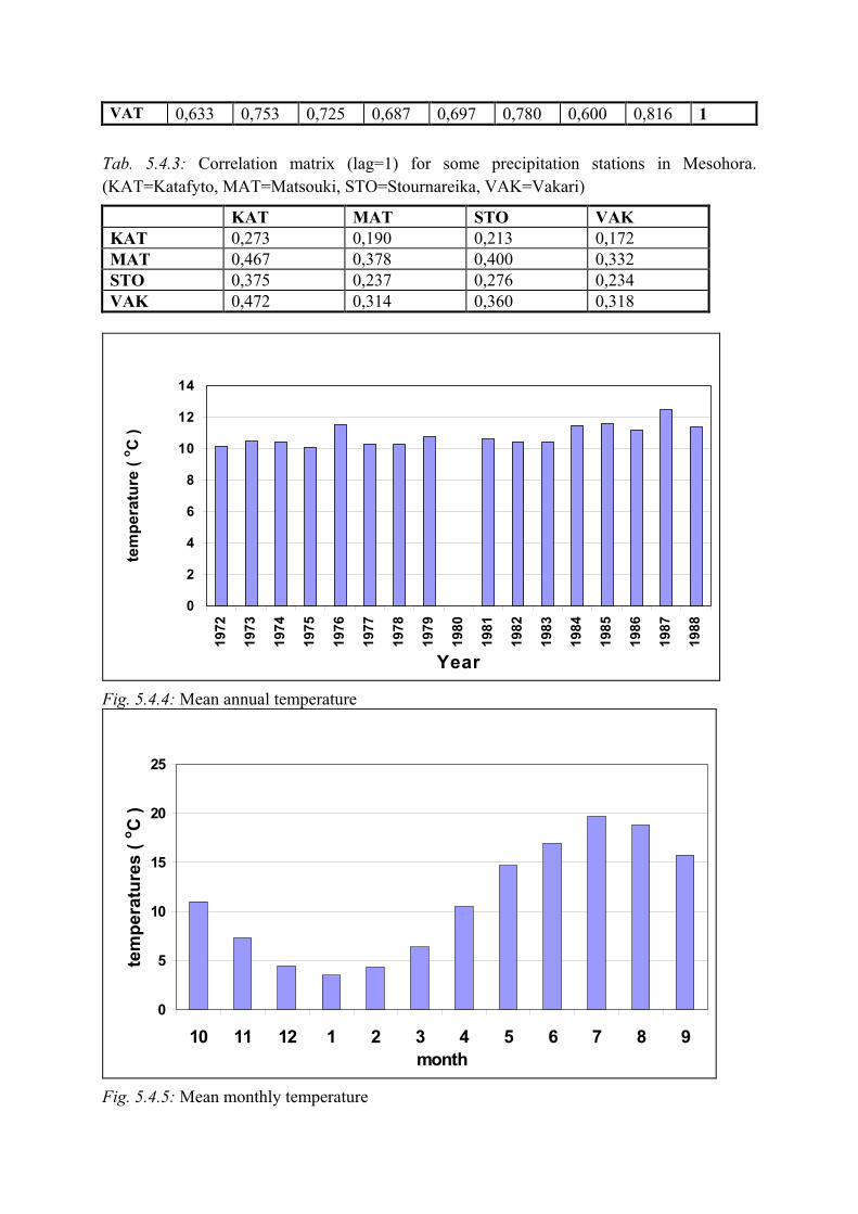
VAT 0,633 0,753 0,725 0,687 0,697 0,780 0,600 0,816 1 Tab. 5.4.3: Correlation matrix (lag=1) for some precipitation stations in Mesohora. (KAT=Katafyto, MAT=Matsouki, STO=Stournareika, VAK=Vakari)

KAT MAT STO VAK KAT 0,273 0,190 0,213 0,172 MAT 0,467 0,378 0,400 0,332 STO 0,375 0,237 0,276 0,234 VAK 0,472 0,314 0,360 0,318

0

2

4

6

8

10

12

14

1972

1973

1974

1975

1976

1977

1978

1979

1980

1981

1982

1983

1984

1985

1986

1987

1988

Year

tem

pera

ture

( o C

)

Fig. 5.4.4: Mean annual temperature

0

5

10

15

20

25

10 11 12 1 2 3 4 5 6 7 8 9month

tem

pera

ture

s ( o C

)

Fig. 5.4.5: Mean monthly temperature

1972

1973

1974

1975

1976

1977

1978

1979

1980

1981

1982

1983

1984

1985

1986

1987

0

500

1000

1500

2000

2500

3000

3500an

nual

pre

cip.

hei

ght (

mm

)

year

PAHTOURI KATAFYTO MATSOUKI PERTOULI VAKARI

Fig. 5.4.6a: Total precipitation height in five stations

0

50

100

150

200

250

300

10 11 12 1 2 3 4 5 6 7 8 9month

prec

ipita

tion

( mm

)

Fig. 5.4.6b: Monthly mean of basin mean precipitation for the period 1972 - 1989

5.4.2.2 Hydrology at the basin scale Except of precipitation, the only measured water balance component in Mesohora basin is total runoff. Fig. 5.4.7 shows the mean annual runoff in the investigated period. Fig. 5.4.8 shows the long term monthly mean of runoff. The largest runoff values appear from

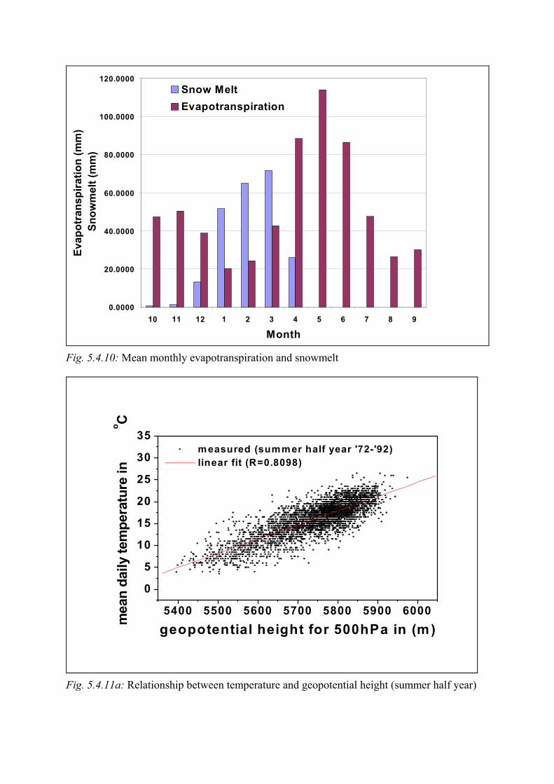
November to March. For the estimation of the water balance components (evapotranspiration, snow melt, surface flow, interflow and base flow) the runoff model ENNS, which has been calibrated for the conditions of the Mesohora basin has been used. Fig. 5.4.9 presents mean monthly values of runoff components (surface flow, interflow and base flow) as they result from the simulation. Surface flow appears only during the winter half year and is small compared to the other components. Interflow exists only from October to April and in this period it is the most important component. Base flow exists over the whole year and has its maximal values from November to May. Fig. 5.4.10 shows the mean monthly values of actual evapotranspiration and snowmelt as they result from the simulation. Evapotranspiration follows the variation of the temperature and the water availability in the soil over the year. The maximal value of evapotranspiration (≈110mm) appears in May. Snowmelt contributes to runoff from December to April. It should be noticed that snowfall data are not available. They were hypothetically determined by considering precipitation measurements as snowfall where temperature falls below zero. The hypothesis is checked so that snow accumulation and water from snowmelt appear together when the measured runoff shows that clearly these processes are taking place.

5.4.2.3 Possible reasons of temperature and precipitation changes in case of increased CO2-concentration

As already seen (Fig. 5.4.1), increased CO2-concentration in the atmosphere causes the increase of pressure. Further it causes changes of the occurrence probability of the weather types. In order to find out if the increase of pressure and the change of the occurrence probability of the weather types cause changes of temperature and precipitation, it is important to investigate if: • there is a functional relationship between geopotential height and local hydrologic

variables (temperature and precipitation) • the value of the local variables depends on the weather types and • the occurrence probability of the weather types changes significantly in case that CO2-

concentration is doubled.

5.4.2.3.1 Dependence of temperature and precipitation on geopotential height Owing to the fact that with increasing CO2-concentration geopotential height of the 500hPa isobar increases, changes of temperature and precipitation at the basin scale should be expected if there is a functional relationship between geopotential height and temperature as well as geopotential height and precipitation. Fig. 5.4.11 shows the relationship between temperature and spatial mean of geopotential height for the Mesohora basin. The correlation is stronger for the summer than for the winter half-year but changes of temperature in Mesohora basin should be expected in both winter and summer half year because of the changes of the geopotential height.

0,00

5,00

10,00

15,00

20,00

25,00

30,00

35,00

1972

1973

1974

1975

1976

1977

1978

1979

1980

1981

1982

1983

1984

1985

1986

1987

1988

Year

Run

off(m

3 /sec

)

Fig. 5.4.7: Mean annual runoff

0

200

400

600

800

1000

1200

1400

10 11 12 1 2 3 4 5 6 7 8 9Month

Run

off (

m3 /s

ec)

Fig. 5.4.8: Monthly mean of measured runoff for the period 1972 – 1989

0.0000

100.0000

200.0000

300.0000

400.0000

500.0000

600.0000

700.0000

800.0000

10 11 12 1 2 3 4 5 6 7 8 9

Month

Run

off (

m3 /s

ec)

Surface FlowInter FlowBase Flow

Fig. 5.4.9: Mean monthly components of runoff

0.0000

20.0000

40.0000

60.0000

80.0000

100.0000

120.0000

10 11 12 1 2 3 4 5 6 7 8 9

Month

Evap

otra

nspi

ratio

n (m

m)

Sno

wm

elt (

mm

)Snow MeltEvapotranspiration

Fig. 5.4.10: Mean monthly evapotranspiration and snowmelt

5400 5500 5600 5700 5800 5900 6000

0

5

10

15

20

25

30

35 measured (summer half year '72-'92) linear fit (R=0.8098)

mea

n da

ily te

mpe

ratu

re in

o C

geopotential height for 500hPa in (m)

Fig. 5.4.11a: Relationship between temperature and geopotential height (summer half year)

5200 5300 5400 5500 5600 5700 5800 5900

-5

0

5

10

15

20

25 measured (w inter half year '72-'92) linear fit (R=0.5759)

mea

n da

ily te

mpe

ratu

re in

0 C

geopotential height for 500 hPa in (m)

Fig. 5.4.11b: Relationship between temperature and geopotential height (winter half year) Fig. 5.4.12 shows that for the station Katafyto in Mesohora there is no functional relationship between precipitation and geopotential height. Similar results have been obtained for all other stations. Additionally, this relationship has been calculated for each weather type of the classification schemes discussed in chapter 5.3.1. Also in this case no better results have been obtained. Consequently, the increase of geopotential height in case of 2*CO2 do not justify changes of precipitation height. For the classification schemes WCS2, WCS3 and WCS4, which are based on the geopotential height gradient, it has been investigated if there is a functional relationship between precipitation and geopotential height gradient. The results shown in Fig. 5.4.13 have been obtained for classification scheme WCS3. The correlation estimated for the weather type 3, which corresponds to geopotential height gradient direction D3 (see Fig 5.3.1), is weak. Similar results have been obtained for the other directions as well as for the classification schemes WCS2 and WCS4. Thus, eventual changes of geopotential height gradients in case of 2*CO2 do not justify changes of precipitation height too.

5.4.2.3.2 Dependence of temperature and precipitation on weather type Owing to the fact that one of the consequences of climate change is the change of the occurrence probability of the different weather types, changes of temperature and precipitation should be expected if these local hydrological variables are related to the weather types. Fig. 5.4.14 shows the dependence of mean daily temperature on the weather types for the classification schemes WCS1, WCS2, WCS3 and WCS4. All classification schemes show that in winter half year, mean daily temperature depends stronger on the weather type than in summer. In all classification schemes, standard deviation (sd) of daily temperature conditioned on the weather type is in the winter half year large compared to the mean value. In the summer half year sd is small. In classification schemes WCS2 and WCS3 the highest temperatures appear for the directions D2, D3 and D4. In classification scheme WCS3 (Fig.

5.4.14(c)) this is valid for cyclonic as well as for anticyclonic conditions. Fig. 5.4.14(c) as well as Fig. 5.4.14(d) demonstrates also that for each weather type temperature for cyclonic conditions is lower than temperature for anticyclonic conditions. Figs. 5.4.15 and 5.4.16 show the dependence of the mean daily precipitation on the weather type for all classification schemes used. In all classification schemes there are dominating weather types. In WCS3 there is a stronger concentration of the large precipitation heights in few weather types (3 and 4 corresponding to geopotential height gradient directions D3 and D4 and cyclonic conditions) than it is the case in WCS1 and WCS2. Particularly in WCS4, large precipitation heights are concentrated in one weather type (weather type 1 corresponding to south, southeast, southwest winds and cyclonic conditions). For WCS3 and WCS4, which according to Table 5.3.4 have the largest performance indices and for this reason they are used below to downscale precipitation according to method of Matyasovszky et al. (1994), the probability of precipitation for the different weather types is given in Fig. 5.4.17. Precipitation probability has been calculated using the mean precipitation in the basin. Fig. 5.4.17(a) shows that in WCS3 the weather types corresponding to geopotential height gradient directions D3 and D4 and to cyclonic conditions are those with significantly higher precipitation probability than the other weather types. Fig. 5.4.17(b) shows that weather type 1 corresponding to south, southeast, southwest winds and cyclonic conditions have significantly higher precipitation probability than all other weather types in classification scheme WCS4.

0 20 40 60 80 100

5300

5400

5500

5600

5700

5800

5900

6000winter half year '72-'89 KATAFYTO (measured) linear fit (R=-0.205)

geop

oten

tial h

eigh

t in

m

precipitation height in mm

Fig. 5.4.12a: Dependence of precipitation height in Katafyto station on geopotential height for 500 hPa (winter half year)

0 10 20 30 40 50 605400

5500

5600

5700

5800

5900

6000summer half year '72-'89

KATAFYTO (measured) linear fit (R=-0.264)

geop

oten

tial h

eigh

t in

m

precipitation height in mm

Fig. 5.4.12b: Dependence of precipitation height in Katafyto station on geopotential height for 500 hPa (summer half year)

0 20 40 60 80 100 120

0

50

100

150

200 linear fit (R=0.36)PAHTOURIwinter half year '72-'89Weather type WT3

daily

pre

cipi

tatio

n in

mm

geopotential height gradient

Fig. 5.4.13: Dependence of precipitation height on geopotential height gradient for the classification scheme WCS3 and weather type 3

5.4.2.3.3 Occurrence probability of weather types Fig. 5.4.18 shows the occurrence probability of the weather types for the classification schemes WCS1, WCS2 and WCS3 whereas Fig. 5.4.19 shows the occurrence probability for

WCS4. Occurrence probability for the historic case is given along with occurrence probability for the cases 1*CO2 and 2*CO2. In all classification schemes there are dominating weather types (weather types with higher occurrence probability than the others). Particularly in classification scheme WCS2 weather types 5, 6, 7 and 8, which correspond to geopotential height gradient directions D5, D6, D7 and D8 in Fig. 5.3.1, have significantly smaller occurrence probability than the other weather types. This was the reason, why these weather types in classification scheme WCS3 were grouped together. In all classification schemes dominating weather types are the same in winter and summer half year. In WCS3 and WCS4 occurrence probability for cyclonic conditions is smaller than occurrence probability for anticyclonic conditions in both winter and summer half year. In 1*CO2 and 2*CO2 case the dominating weather types in all classification schemes are the same as for the historic data. The differences between the occurrence probability of historic and 1*CO2 case are for all classification schemes larger than the differences between 1*CO2 and 2*CO2. This is a further indication that the quality of the used GCM results is questionable, as 1*CO2 case should be closer to the historic than to 2*CO2 case.

1 2 3 4 5 6 7 8 9 100

1

2

3

4

5

6

7

8

9winter half year '72-'92

mea

n da

ily te

mpe

ratu

re in

0 C

Weather type

mean sd

1 2 3 4 5 6 7 8 9 1002468

101214161820

summer half year '72-'92m

ean

daily

tem

pera

ture

in 0 C

Weather type

mean sd

Fig. 5.4.14a: Dependence of mean daily temperature on weather type for classification WCS1

1 2 3 4 5 6 7 80

1

2

3

4

5

6

7

8

9winter half year '72-'92

mea

n da

ily te

mpe

ratu

r in

0 C

Weather type

mean sd

1 2 3 4 5 6 7 8 9 1002468

101214161820

mean sdsummer half year '72-'92

mea

n da

ily te

mpe

ratu

re in

0 C

Weather type

Fig. 5.4.14b: Dependence of mean daily temperature on weather type for classification WCS2

( b )

1 2 3 4 5 6 7 8 9 100

1

2

3

4

5

6

7

8

9 mean sdwinter half year '72-'92

mea

n da

ily te

mpe

ratu

re in

0 C

Weather type1 2 3 4 5 6 7 8 9 10

02468

101214161820

mean sdsummer half year '72-'92

mea

n da

ily te

mpe

ratu

re in

0 C

Weather type

Fig. 5.4.14c: Dependence of mean daily temperature on weather type for classification WCS3

1 20

2

4

6

8

10

12

14

16

18

20

22

24

mea

n da

ily te

mpe

ratu

re in

n0 C

Weather type

mean sd (winter half year '72-'92) mean sd (summer half year '72-'92)

Fig. 5.4.14d: Dependence of mean daily temperature on weather type for classification WCS4

1 2 3 4 5 6 7 8 9 100

2

4

6

8

10

12

14

16

18

20

22

Weather type

KatafytoMatsoukiPahtouriPaliochoriPertouliStournar.TyrnaVakari

Mean dailyprecipitationheight(mm)

Fig. 5.4.15a: Dependence of precipitation height on weather type for classification WCS1

1 2 3 4 5 6 7 802468

101214161820

winter half year '72 - '89

mea

n da

ily p

reci

pita

tion

(mm

)

Weather type

Katafyto Matsouki Pahtouri Paleohori Pertouli Stournareik Tyrna Vakari Vathyrema

Fig. 5.4.15b: Dependence of precipitation height on weather type for classification WCS2

1 2 3 40

1

2

3

4

5

6

7 summer '72-'89

mea

n da

ily p

reci

pita

tion

(mm

)

WT

KAT MAT PAH PAL PER STO TYR VAK VAT

1 2 3 4 5 6 7 8 9 1002468

1012141618202224262830

winter half year '72-'89

mea

n da

ily p

reci

pita

tion

in m

m

Weather type


Fig. 5.4.16a: Dependence of precipitation height on weather type for classification WCS3

1 2 3 4 5 6 7 8 9 100123456789

10111213

summer half year '72-'89

mea

n da

ily p

reci

pita

tion

in m

m

Weather type


1 2 3 40

2

4

6

8

10

12

14

16

18

20

22

24 winter '72-'89m

ean

daily

pre

cipi

tatio

n (m

m)

weather type


Fig. 5.4.16b: Dependence of precipitation height on weather type for classification WCS4

1 2 3 4 5 6 7 8 9 100 .0

0 .1

0 .2

0 .3

0 .4

0 .5

0 .6

0 .7

0 .8

prob

abili

ty o

f pre

cipi

tatio

n

W ea th e r typ e

w in te r h a lf ye ar '7 2 -'89 su m m er h a lf year '72 -'8 9

Fig. 5.4.17a: Probability of precipitation for classification concept WCS3

1 2 3 40 .0

0 .1

0 .2

0 .3

0 .4

0 .5

0 .6

0 .7

0 .8pr

obab

ility

of p

reci

pita

tion

w ea th e r typ e

w in te r h a lf ye a r '7 2 - '8 9 s u m m e r h a lf ye a r '7 2 - '8 9

Fig. 5.4.17b: Probability of precipitation for classification concept WCS4

5.4.2.4 Validation of the downscaling approach In this study the downscaling approach proposed by Matyasovszky et al. (1994) has been used. For validation the method has been used to calculate cumulative probabilities of measured temperature and precipitation. The results have been compared with the cumulative probabilities resulting from the data. Validation presented below concerns classification schemes WCS3 and WCS4, which have the largest performance indices (Table 5.3.4). Results obtained by using classification scheme WCS1 have been presented in the Annex of Second Annual Report of this project. WCS2 gives similar results as WCS3. Therefore it is not discussed separately.

5.4.2.4.1 Downscaling of temperature and precipitation based on WCS3 Fig. 5.4.20 shows the cumulative probability estimated from the temperature data and from the simulation using the method of Matyasovsky et al. (1994) for November, March, April and September. Similar results have been obtained for all months of the year. In Table 5.4.4 the differences between measured and simulated cumulative probabilities are given. For some months these differences are 1.50C and appear over the whole range of the temperature values. Owing to the fact that the expected changes of temperature in 2*CO2 case are of the order of 20C, the error of the downscaling model in simulating the historic data is not negligible. It is of the order of climate change impact. The most probable reason for this error is that in Mesohora basin, temperature distribution conditioned on the weather types is not binormal. Chi-square tests showed that in many cases the conditioned empirical temperature distribution could not be approximated appropriately by the binormal distribution for the usual significance level of 5%.

Tab. 5.4.4: Comparison between measured and simulated cumulative probability of temperature

DIFFERENCE BETWEEN SIMULATED AND MEASURED TEMPERATURE IN OC

REMARKS

October +0,20 over the whole interval of values November +1,50 over the whole interval of values December +1,50 over the whole interval of values January +0,50 over the whole interval of values February +1,50 over the whole interval of values March ----- ----- April +1,50 over the upper interval of values May +1,50 over the upper interval of values June +0,50 over the whole interval of values July +1,10 over the whole interval of values August +0,50 over the whole interval of values September +0,50 over the lower interval of values

Fig. 5.4.21 shows the cumulative probability estimated from precipitation data and simulated using the model of Matyasovszky et al. (1994) for four stations in the Mesohora basin. The model does not approximate the cumulative probability of historic data appropriately. This occurs particularly for small precipitation heights.

1 2 3 4 5 6 7 8 9 100.000.020.040.060.080.100.120.140.160.180.20

winter half year

occu

rren

ce p

roba

bilit

y

Weather type

historic '72-'89 1xCO2 2xCO2

1 2 3 4 5 6 7 8 9 100.00

0.02

0.04

0.06

0.08

0.10

0.12

0.14

0.16

0.18summer half year

occu

rren

ce p

roba

bilit

y

Weather type


Fig. 5.4.18a: Occurrence probability of different weather types for classification concept WCS1

1 2 3 4 5 6 7 8 9 100.000.020.040.060.080.100.120.140.160.180.200.22

winter half yearoc

curr

ence

pro

babi

lity

Weather type


1 2 3 4 5 6 7 80.000.050.100.150.200.250.300.350.400.45 summer half year

occu

rren

ce p

roba

bilit

y

Weather type

hisroric '72-'92 1xCO2 2xCO2

Fig. 5.4.18b: Occurrence probability of different weather types for classification concept WCS2

1 2 3 4 5 6 7 80.00

0.05

0.10

0.15

0.20

0.25

0.30

0.35 winter half year

occu

rren

ce p

roba

bilit

y

Weather type


1 2 3 4 5 6 7 8 9 100.00

0.05

0.10

0.15

0.20

0.25 summer half year

occu

rren

ce p

roba

bilit

y

Weather type


Fig. 5.4.18c: Occurrence probability of different weather types for classification concept WCS3

1 20.0

0.1

0.2

0.3

0.4

0.5

0.6

0.7

winter

occu

rren

ce p

roba

bilit

y

Weather type


1 20.0

0.1

0.2

0.3

0.4

0.5

0.6

summer

occu

rrenc

e pr

obab

ility

Weather type


Fig. 5.4.19a: Occurrence probability of different weather types for classification concept WCS4

1 2 3 40.00

0.05

0.10

0.15

0.20

0.25

0.30

0.35

0.40summer

occu

rren

ce p

roba

bilit

y

WT


1 2 3 40.00

0.05

0.10

0.15

0.20

0.25

0.30

0.35

0.40

winter

occu

rren

ce p

roba

bilit

y

Weather type


Fig. 5.4.19b: Occurrence probability of different weather types for classification concept WCS4

-10 -5 0 5 10 15 20 25 30

0

20

40

60

80

100 November

historic '72-'92 simulated

cum

ulat

ive

prob

abili

ty

temperature in0C

-10 -5 0 5 10 15 20 25 30

0

20

40

60

80

100 March


cum

ulat

ive

prob

abili

ty

temperature in 0C

Fig. 5.4.20a: Cumulative probability for temperature in November and March

-10 -5 0 5 10 15 20 25 30

0

20

40

60

80

100 April


cum

ulat

ive

prob

abili

ty

temperature in 0C

-10 -5 0 5 10 15 20 25 30

0

20

40

60

80

100September


cum

ulat

ive

prob

abili

ty

temperature in 0C

Fig. 5.4.20b: Cumulative probability for temperature in April and September

The most probable reason for these deviations is the small number of days belonging to each weather type due to the relatively large number of weather types considered in this classification scheme combined with the relatively short precipitation time series, which are available.

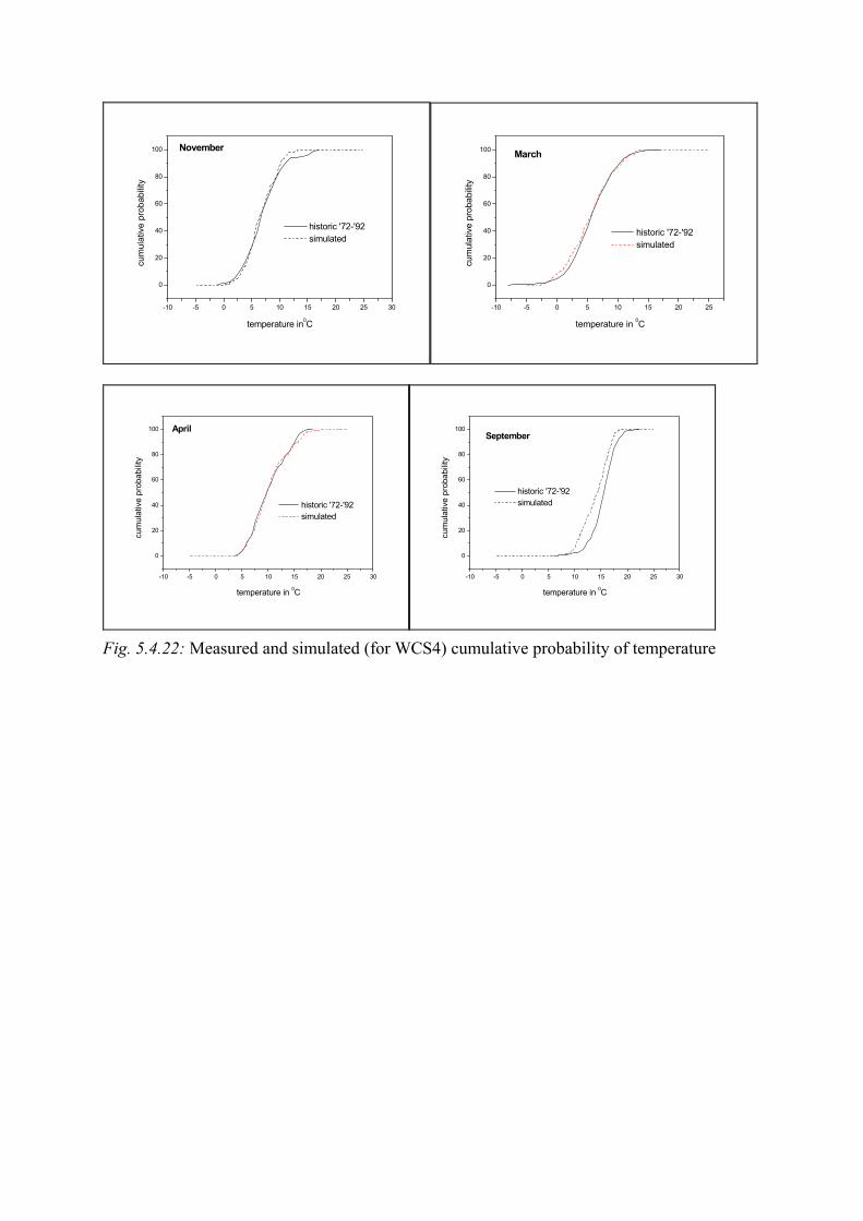
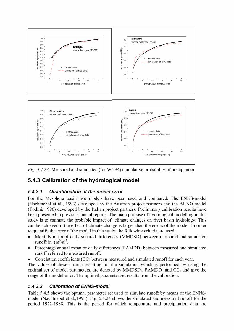
5.4.2.4.2 Downscaling of temperature and precipitation based on WCS4 For WCS4, the cumulative probability estimated from the temperature data and from the simulation for November, March April and September is shown in Fig. 5.4.22. Comparing Figs. 5.4.20 and 5.4.22 it can be seen that WCS4 does not give better results than WCS3. This is valid for all months of the year. Investigation of temperature distribution conditioned on weather types for WCS4 has shown that also for this classification, the distribution is not binormal. This is the most probable reason for the deviations between measured and simulated occurrence probability. Fig. 5.4.23 shows the measured and simulated occurrence probability for WCS4 and for the same stations as those in Fig. 5.4.22 for WCS3. Comparing the results in Figs. 5.4.22 and 5.4.23 it can be seen that for WCS4 the model approximates the precipitation cumulative probability much better than for WCS3. The most probable reason is that in WCS4, the number of weather types is smaller than in WCS3 and consequently the number of days belonging to each weather type is larger than in WCS3. However, also for WCS4 there are no negligible deviations between measured and simulated cumulative probability of precipitation.

0 10 20 30 40 500.65

0.70

0.75

0.80

0.85

0.90

0.95

1.00

Katafytowinter half year '72-'87

historic data simulation of hist. dataoc

curr

ence

pro

babi

lity

precipitation height (mm)0 10 20 30 40 50

0.5

0.6

0.7

0.8

0.9

1.0

Matsoukiwinter half year '72-'87

historic data simulation of hist. data

occu

rren

ce p

roba

bilit

y

precipitation height (mm)

0 10 20 30 40 500.55

0.60

0.65

0.70

0.75

0.80

0.85

0.90

0.95

1.00

Stournareika winter half year '72-'87


occu

rrenc

e pr

obab

ility


0.5

0.6

0.7

0.8

0.9

1.0

Vakari winter half year '72-'87


curr

ence

pro

babi

lity


Fig. 5.4.21: Measured and simulated (for WCS3) cumulative probability of precipitation

-10 -5 0 5 10 15 20 25 30

0

20

40

60

80

100 November


cum

ulat

ive

prob

abilit

y

temperature in0C

-10 -5 0 5 10 15 20 25

0

20

40

60

80

100 March


cum

ulat

ive

prob

abilit

y

temperature in 0C

-10 -5 0 5 10 15 20 25 30

0

20

40

60

80

100 April


cum

ulat

ive

prob

abilit

y

temperature in 0C

-10 -5 0 5 10 15 20 25 30

0

20

40

60

80

100September


cum

ulat

ive

prob

abilit

y

temperature in 0C

Fig. 5.4.22: Measured and simulated (for WCS4) cumulative probability of temperature

0 10 20 30 40 50

0.40

0.45

0.50

0.55

0.60

0.65

0.70

0.75

0.80

0.85

0.90

0.95

1.00

Katafyto winter half year '72-'87


curr

ence

pro

babi

lity


0.5

0.6

0.7

0.8

0.9

1.0 Matsouki winter half year '72-'87


occu

rren

ce p

roba

bilit

y


0 10 20 30 40 50

0.55

0.60

0.65

0.70

0.75

0.80

0.85

0.90

0.95

1.00 Stournareika winter half year '72-'87


occu

rrenc

e pr

obab

ility


0.5

0.6

0.7

0.8

0.9

1.0 Vakari winter half year '72-'87


occu

rren

ce p

roba

bilit

y


Fig. 5.4.23: Measured and simulated (for WCS4) cumulative probability of precipitation

5.4.3 Calibration of the hydrological model

5.4.3.1 Quantification of the model error For the Mesohora basin two models have been used and compared. The ENNS-model (Nachtnebel et al., 1993) developed by the Austrian project partners and the ARNO-model (Todini, 1996) developed by the Italian project partners. Preliminary calibration results have been presented in previous annual reports. The main purpose of hydrological modelling in this study is to estimate the probable impact of climate changes on river basin hydrology. This can be achieved if the effect of climate change is larger than the errors of the model. In order to quantify the error of the model in this study, the following criteria are used: • Monthly mean of daily squared differences (MMDSD) between measured and simulated

runoff in (m3/s)2. • Percentage annual mean of daily differences (PAMDD) between measured and simulated

runoff referred to measured runoff. • Correlation coefficients (CC) between measured and simulated runoff for each year. The values of these criteria resulting for the simulation which is performed by using the optimal set of model parameters, are denoted by MMDSD0, PAMDD0 and CC0 and give the range of the model error. The optimal parameter set results from the calibration.

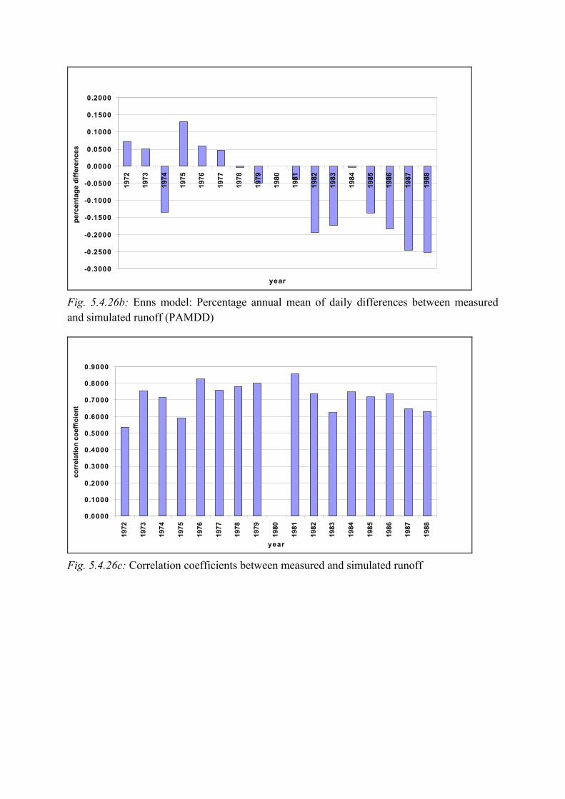
5.4.3.2 Calibration of ENNS-model Table 5.4.5 shows the optimal parameter set used to simulate runoff by means of the ENNS-model (Nachtnebel et al.,1993). Fig. 5.4.24 shows the simulated and measured runoff for the period 1972-1988. This is the period for which temperature and precipitation data are

available. Fig. 5.4.25 shows the simulation results for three years (1972-1973, 1981-1982, and 1983-1984). In both figures there is generally good agreement between measurements and simulation, particularly in the dry period of the year. Snowmelt can not be simulated reliably as it results from the simulation of the year 1983-1984. High values of measured runoff in May are probably caused by snowmelt, as precipitation during this period is not significant. This effect can not be described by the model because, as already referred, snowfall data are not available. Fig. 5.4.26 shows MMDSD0, PAMDD0 and CC0 for the investigated period. The largest values of MMDSD0 result for the period of the year with the highest precipitation (compare Fig. 5.4.6). Correlation coefficients are for the most years larger than 0.7, which corresponds to a relatively high correlation. The maximal value of PAMDD0 is 25%. The most PAMDD0 values are less than 15%. Tab. 5.4.5: Optimal set of model parameters for ENNS-model.

PARAMETER SYMBOL VALUE Field Capacity FK 0,20 Wilting point PWP 0,12 Thickness of soil layer M 4000,00 (mm) Infiltration parameter BETA 5,50 Constant for soil moist. reduction

KBF 4000,00

Threshold value for reservoir 1 H1 5,0 (mm) Threshold value for reservoir 2 H2 20,0 (mm) Constant for reservoir 1 TVS1 5,0 (hr) Constant for reservoir 2 TVS2 259,0 (hr) Storage factor for reservoir 1 TAB1 5 ,0 (hr) Storage factor for reservoir 2 TAB2 78,0 (hr) Storage factor for reservoir 3 TAB3 300 ,0 (hr) Storage factor for reservoir 4 TAB4 5, 0 (hr) Min. soil temperature TSOILMIN - 5,0 (OC) Max. soil temperature TSOILMAX 25 (OC) New snow height variance Zone 1 Zone 2-3 Zone 4

VAR 0,250 (mm) 0,319 (mm) 1,693 (mm)

Maximal degree – day factor Zone 1, 2 Zone 3, 4

CTMAX 2,30 (mm/oC) 9,30 (mm/oC)

Minimal degree - day factor CTMIN 0,50 (mm/oC) Degree – day factor for melting CTNEG 0,50 Snow max. density SHROMAX 0,50

0

5 0

1 0 0

1 5 0

2 0 0

2 5 0

3 0 0

3 5 0

4 0 0

4 5 0

1

258

515

772

1029

1286

1543

1800

2057

2314

2571

2828

3085

3342

3599

3856

4113

4370

4627

4884

5141

5398

5655

5912

6169

d a y s

Run

off(m

3 /sec

)m e a s u r e ds i m u l a t e d

Fig. 5.4.24: Runoff measured and simulated by means of the Enns model for the period 1972-1988

Y e a r 1 9 7 2 - 7 3

0

5 0

1 0 0

1 5 0

2 0 0

2 5 0

3 0 0

3 5 0

4 0 0

4 5 0

1 17 33 49 65 81 97 113

129

145

161

177

193

209

225

241

257

273

289

305

321

337

353

d a y s

Run

off(m

3 /sec

)

m e a s u r e ds i m u l a t e d

Y e a r 1 9 8 1 -8 2

0

5 0

1 0 0

1 5 0

2 0 0

2 5 0

3 0 0

3 5 0

4 0 0

4 5 0

1 16 31 46 61 76 91 106

121

136

151

166

181

196

211

226

241

256

271

286

301

316

331

346

361

d a y s

Run

off(m

3 /sec

) m e a s u re ds im u la te d

Y e a r 1 9 8 3 -8 4

0

5 0

1 0 0

1 5 0

2 0 0

2 5 0

3 0 0

3 5 0

4 0 0

4 5 0

1 17 33 49 65 81 97 113

129

145

161

177

193

209

225

241

257

273

289

305

321

337

353

d a y s

Run

off(m

3 /sec

) m e a s u re ds im u la te d

Fig. 5.4.25: Runoff measured and simulated by means of the Enns model for the period

5.4.3.3 Calibration of ARNO-model Simulation of runoff in the Mesohora basin by means of the ARNO-model using daily values of precipitation have been presented in the previous annual report. Here an attempt has been undertaken in order to improve the simulation by using, instead of daily, hourly values of precipitation. Hourly time steps are more consistent with the concentration time of the Mesohora basin, which is less than 24 hours. For this purpose daily precipitation values were distributed uniformly over the 24 hours. In Table 5.4.6 the optimal combination of the parameters used for the simulation on daily and hourly basis are given. Tab. 5.4.6: Calibrated parameter values for ARNO-model.

PARAMETER VALUE FOR DT=1D

VALUE FOR DT=1H

potential evapotranspiration (AL,BE) 1.6935, 0.5749 1.6935, 0.5749 field capacity in mm (WM) 50.0 50.0 soil saturation rating curve exponent (B) 1.0 0.2 drainage maximum value in mm/h (DRMAX) 2.0 1.0 drainage exponent (CESP) 2.0 1.0 drainage base curve maximum in mm/h (DRMIN)

0.03 0.1

drainage threshold in mm (SOL) 230.0 130.0 threshold in mm (SOL1) 30.0 30.0 percolation maximum in mm/h (PERC) 1.1 4.0 percolation exponent (PESP) 2.0 0.5 groundwater linear reservoir number (NP) 1 1 groundwater linear reservoir constant in h (KFA) 1.0 1.0 snow threshold temperature (TS) 0.0 0.0

0

5 0 0 0

1 0 0 0 0

1 5 0 0 0

2 0 0 0 0

2 5 0 0 0

3 0 0 0 0

3 5 0 0 0

4 0 0 0 0

4 5 0 0 0

1 0 1 1 1 2 1 2 3 4 5 6 7 8 9m o n th

squa

red

diffe

renc

es (m

3 /sec

)2

Fig. 5.4.26a: Enns model: Monthly mean of daily squared differences between measured and simulated runoff (MMDSD)

-0.3000

-0.2500

-0.2000

-0.1500

-0.1000

-0.0500

0.0000

0.0500

0.1000

0.1500

0.2000

1972

1973

1974

1975

1976

1977

1978

1979

1980

1981

1982

1983

1984

1985

1986

1987

1988

year

perc

enta

ge d

iffer

ence

s

Fig. 5.4.26b: Enns model: Percentage annual mean of daily differences between measured and simulated runoff (PAMDD)

0.0000

0.1000

0.2000

0.3000

0.4000

0.5000

0.6000

0.7000

0.8000

0.9000

1972

1973

1974

1975

1976

1977

1978

1979

1980

1981

1982

1983

1984

1985

1986

1987

1988

year

corr

elat

ion

coef

ficie

nt

Fig. 5.4.26c: Correlation coefficients between measured and simulated runoff

Year 1972-73

0

50

100

150

200

250

300

350

400

450

1 22 43 64 85 106

127

148

169

190

211

232

253

274

295

316

337

358

days

runo

ff ( m

3 /sec

)

measuredsimulated

Year 1981-82

0

50

100

150

200

250

300

350

400

450

1 21 41 61 81 101

121

141

161

181

201

221

241

261

281

301

321

341

361

days

runo

ff ( m

3 /sec

)

measuredsimulated

Year 1983-84

0

50

100

150

200

250

300

350

400

450

1 21 41 61 81 101

121

141

161

181

201

221

241

261

281

301

321

341

361

days

runo

ff ( m

3 /sec

)

measuredsimulated

Fig. 5.4.27: Simulation of runoff by means of ARNO model using one day time steps

Year 1972-73

0

50

100

150

200

250

300

350

400

450

1 21 41 61 81 101

121

141

161

181

201

221

241

261

281

301

321

341

361

days

runo

ff ( m

3 /sec

)

measuredsimulated

Year 1981-82

0

50

100

150

200

250

300

350

400

450

1 24 47 70 93 116 139 162 185 208 231 254 277 300 323 346days

runo

ff ( m

3 /sec

)

measuredsimulated

Year 1983-84

0

50

100

150

200

250

300

350

400

450

1 21 41 61 81 101

121

141

161

181

201

221

241

261

281

301

321

341

361

days

runo

ff (m

3/se

c ) measured

simulated

Fig. 5.4.28: Simulation of runoff by means of ARNO model using one hour time steps

period : 1972 - 1989

0

10000

20000

30000

40000

50000

60000

10 11 12 1 2 3 4 5 6 7 8 9month

squa

red

diffe

renc

es (

m3 /s

ec )2

Fig. 5.4.29a: Monthly mean of daily squared differences between measured and simulated (by means of ARNO model) runoff for one day time step

period : 1972 - 1989

0

10000

20000

30000

40000

50000

60000

10 11 12 1 2 3 4 5 6 7 8 9month

squa

red

diffe

renc

es (

m3 /s

ec)2

Fig. 5.4.29b: Monthly mean of daily squared differences between measured and simulated (by means of ARNO model) runoff for one hour time step The optimal values of the parameters B, DRMAX, CESP, DRMIN, SOL, PERC and PESP resulted for one-day and one-hour time steps are considerably different. Fig. 5.4.27 shows the results of simulation for three years (1972-1973, 1981-1982, and 1983-1984) based on one day time steps. Fig. 5.4.28 shows the corresponding results based on one hour time step. For the one hour time step the reaction of the basin to rainfall is much more intensive (quick increase and decrease of runoff, large peaks) than measured runoff shows, although the parameter combination used almost eliminates the surface runoff component. Runoff includes

only interflow and base flow. A possibility to overcome this problem is to use parameters, which reduce drastically interflow and transform it to base flow. However, strong reduction of interflow does not correspond to the conditions in the basin studied. MMDSD values given in Fig. 5.4.29 are generally smaller for one day time step. On the other hand PAMDD values given in Fig. 5.4.30 are smaller for the simulation with one hour time step. Finally, correlation coefficients for one day time steps are larger than the corresponding values for one hour time steps as Fig. 5.4.31 shows. MMDSD values of ARNO model for one day time steps are smaller than the corresponding values of ENNS-model as it results from the comparison of Figs. 5.4.26(a) and 5.4.29(a). Correlation coefficients of both models are comparable (see Fig. 5.4.26(c) and 5.4.31(a)), whereas PAMDD values are better for the ENNS-model (see Fig. 5.4.26(b) and 5.4.30(a)). Thus, the quality of simulation results obtained by means of the ENNS and the ARNO model for one day time steps are comparable.

-0,8

-0,6

-0,4

-0,2

0

0,2

0,4

1972

1973

1974

1975

1976

1977

1978

1979

1980

1981

1982

1983

1984

1985

1986

1987

1988

year

perc

enta

ge d

iffer

ence

s

Fig. 5.4.30a: Percentage annual mean of daily differences between measured and simulated runoff for one day time step

-0,1

-0,05

0

0,05

0,1

0,15

0,2

0,25

0,3

0,35

0,4

1972

1973

1974

1975

1976

1977

1978

1979

1980

1981

1982

1983

1984

1985

1986

1987

1988

year

perc

enta

ge d

iffer

ence

s

Fig. 5.4.30b: Percentage annual mean of daily differences between measured and simulated runoff for one hour time step

00,1

0,20,3

0,40,5

0,60,7

0,80,9

1

1972

1973

1974

1975

1976

1977

1978

1979

1980

1981

1982

1983

1984

1985

1986

1987

1988

year

corr

elat

ion

coef

ficie

nt

Fig. 5.4.31a: Correlation coefficient between measured and simulated runoff for one day time step

0

0,1

0,2

0,30,4

0,5

0,6

0,7

0,8

0,91

1972 1974 1976 1978 1980 1982 1984 1986 1988year

corr

elat

ion

coef

ficie

nt

Fig. 5.4.31b: Correlation coefficient between measured and simulated runoff for one hour time step

5.5 Impact studies (2*CO2)

5.5.1 Changes in geopotential height and in the occurrence probabilities of the weather types

The change of the geopotential height in 2*CO2 case compared to historic data has already been discussed in chapter 5.4.1. However, the estimation of the cumulative probability of temperature and precipitation for the 2*CO2 case according to Matyasovszky et al. (1994), is not performed by using the original GCM output but by using values which are reduced analogously to the difference between historic and 1*CO2 values. Thus, the increase of geopotential height, by means of which the calculation of cumulative probability of temperature and precipitation in 2*CO2 case is carried out, is less than that given in Table 5.4.1. The occurrence probabilities for the classification schemes WCS3 and WCS4 in 2*CO2 case are given in Fig. 5.4.18. They differ from the corresponding values of the historic case less than 10%. However, it should be noticed that the occurrence probabilities in 1*CO2 case, which result from the GCM geopotential heights, are probably overestimated just as they are closer to 2*CO2 case than to historic case. Therefore occurrence probabilities of 2*CO2 case can be overestimated too. Thus, their difference from the historic case can be smaller than shown in Fig. 5.4.18. The smaller are the differences between historic and 2*CO2 case, the smaller changes of the cumulative probability of temperature and precipitation in 2*CO2 case compared to the historic case must be expected.

5.5.2 Hydrometeorological impact of climate change on basin

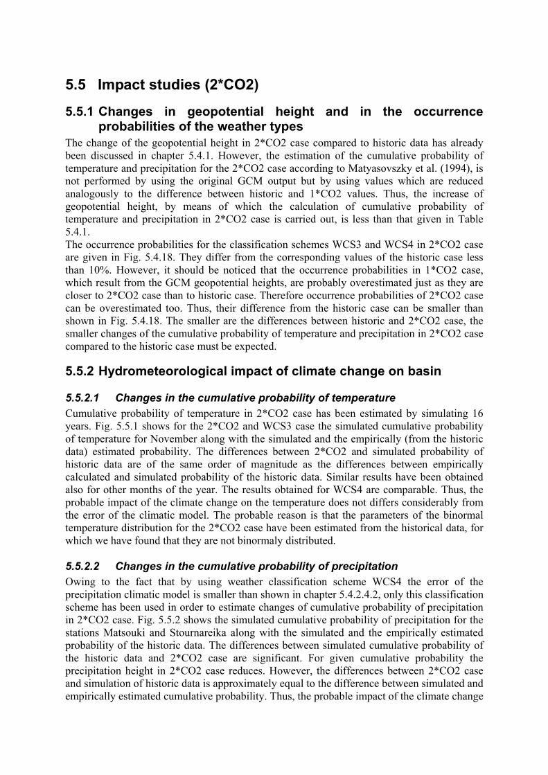
5.5.2.1 Changes in the cumulative probability of temperature Cumulative probability of temperature in 2*CO2 case has been estimated by simulating 16 years. Fig. 5.5.1 shows for the 2*CO2 and WCS3 case the simulated cumulative probability of temperature for November along with the simulated and the empirically (from the historic data) estimated probability. The differences between 2*CO2 and simulated probability of historic data are of the same order of magnitude as the differences between empirically calculated and simulated probability of the historic data. Similar results have been obtained also for other months of the year. The results obtained for WCS4 are comparable. Thus, the probable impact of the climate change on the temperature does not differs considerably from the error of the climatic model. The probable reason is that the parameters of the binormal temperature distribution for the 2*CO2 case have been estimated from the historical data, for which we have found that they are not binormaly distributed.

5.5.2.2 Changes in the cumulative probability of precipitation Owing to the fact that by using weather classification scheme WCS4 the error of the precipitation climatic model is smaller than shown in chapter 5.4.2.4.2, only this classification scheme has been used in order to estimate changes of cumulative probability of precipitation in 2*CO2 case. Fig. 5.5.2 shows the simulated cumulative probability of precipitation for the stations Matsouki and Stournareika along with the simulated and the empirically estimated probability of the historic data. The differences between simulated cumulative probability of the historic data and 2*CO2 case are significant. For given cumulative probability the precipitation height in 2*CO2 case reduces. However, the differences between 2*CO2 case and simulation of historic data is approximately equal to the difference between simulated and empirically estimated cumulative probability. Thus, the probable impact of the climate change

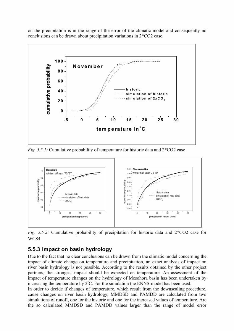
on the precipitation is in the range of the error of the climatic model and consequently no conclusions can be drawn about precipitation variations in 2*CO2 case.

-5 0 5 10 1 5 20 2 5 30

0

2 0

4 0

6 0

8 0

10 0N o vem b er

h is to ric s im u la tio n o f h is to ric s im u la tio n o f 2xC O 2

cum

ulat

ive

prob

abili

ty

tem p era tu re in 0C

Fig. 5.5.1: Cumulative probability of temperature for historic data and 2*CO2 case

0 10 20 30 40 50

0.5

0.6

0.7

0.8

0.9

1.0 Matsoukiwinter half year '72-'87

historic data simulation of hist. data 2xCO2oc

curr

ence

pro

babi

lity


0.55

0.60

0.65

0.70

0.75

0.80

0.85

0.90

0.95

1.00 Stournareika winter half year '72-'87

historic data simulation of hist. data 2XCO2

occu

rren

ce p

roba

bilit

y


Fig. 5.5.2: Cumulative probability of precipitation for historic data and 2*CO2 case for WCS4

5.5.3 Impact on basin hydrology Due to the fact that no clear conclusions can be drawn from the climatic model concerning the impact of climate change on temperature and precipitation, an exact analysis of impact on river basin hydrology is not possible. According to the results obtained by the other project partners, the strongest impact should be expected on temperature. An assessment of the impact of temperature changes on the hydrology of Mesohora basin has been undertaken by increasing the temperature by 2°C. For the simulation the ENNS-model has been used. In order to decide if changes of temperature, which result from the downscaling procedure, cause changes on river basin hydrology, MMDSD and PAMDD are calculated from two simulations of runoff, one for the historic and one for the increased values of temperature. Are the so calculated MMDSD and PAMDD values larger than the range of model error

MMDSD0 and PAMDD0 given in Fig. 5.4.26, then it can be considered that the change of temperature or precipitation has an impact on river basin hydrology. Fig. 5.5.3 shows the percentage annual mean of daily differences (PAMDD) estimated from the simulation for the increased temperature (case T+∆T) and the simulation for the historic temperature data (case T). The differences are less than 9% and consequently they are less than the model error PAMDD0 given in Fig. 5.4.26(b)). Monthly mean of daily squared differences (MMDSD) estimated from the simulations for case T and case (T+ ∆T) shown in Fig. 5.5.4, are much smaller than the values of MMDSD0 given in Fig. 5.4.26(a). Owing to the fact that the optimal set of model parameters on which the values of PAMDD0 and MMDSD0 depends, have been estimated empirically by trial and error, it can not be excluded that there exists an other parameter set that gives values of PAMDD0 and MMDSD0 smaller than those estimated from the simulation of the cases T and T+∆T. In order to investigate if there exists such a parameter set, which reduces the range of the model error, an optimal parameter set has been estimated separately for each of the 17 years, for which data exist. The parameters optimised were the thickness of the soil zone and the field capacity of this zone, which have the strongest influence on total runoff. The criterion of the optimization was to minimise the value of PAMDD0 and MMDSD0 separately. Thus, for each year the thickness of the soil zone and the field capacity have been varied systematically, as shown in Fig. 5.5.5, and the parameter combination minimizing each of the aforementioned criteria has been selected. For those optimal parameter combinations a further control has been made, based on the value of the correlation coefficient in each year and the agreement between measured and simulated time series, which has been checked optically. If for a year the last two controls were not satisfactory, an other parameter set, which is close to the optimal but satisfies the additional criteria (correlation coefficient and agreement of time series), has been found. Table 5.5.1 gives the values satisfying all the aforementioned criteria in each year. The values of PAMDD0 and MMDSD0 estimated for each year by using the values in Table 5.5.1 are given in Fig. 5.5.6. For some of the years result the same parameter sets.

Tab. 5.5.1: Optimal values of soil zone thickness and field capacity for each year.

72 73 74 75 76 77 78 79 80 81 82 83 84 85 86 87 88

m 5 5 5 5 5 5 4 1 2 2 5 1 4 1 2 1 1 Min PAMDD0 Fk 0.2 0.2 0.3 0.2 0.2 0.3 0.2 0.2 0.2 0.3 0.3 0.2 0.2 0.2 0.2 0.2 0.2

m 5 3 1 3 5 3 3 5 5 1 2 1 3 1 2 2 1 Min MMDSD0

Fk 0.2 0.2 0.2 0.2 0.3 0.3 0.2 0.2 0.2 0.4 0.2 0.4 0.2 0.3 0.2 0.2 0.2

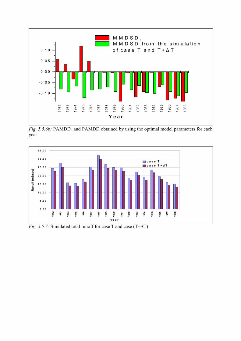
In Fig. 5.5.6 the values of PAMDD and MMDSD estimated for 2°C temperature increase are given along with PAMDD0 and MMDSD0. It can be seen (Fig. 5.5.6(a)) that MMDSD values are still significantly smaller than MMDSD0 values. Thus, it can be practically excluded that the effect of a temperature increase of 20C on runoff process is larger than the model error if MMDSD0 is used as criterion. On the other hand Fig. 5.5.6(b) shows that for the most of the years (11 out of 17) PAMDD is larger than PAMDD0. Thus, based on PAMDD0 an impact of climate change resulting from 2°C-temperature increase can be concluded. However, considering that this was possible only by using different parameter sets for the simulation of different periods, indicates the difficulty to identify the impact of a 2°C-temperature increase also by using the PAMDD criterion.

0,00

0,01

0,02

0,03

0,04

0,05

0,06

0,07

0,08

0,09

0,10

1 2 3 4 5 6 7 8 9 10 11 12 13 14 15 16 17year

perc

enta

ge d

iffer

ence

s

Fig. 5.5.3: Percentage annual mean daily differences between simulated runoff in case T and simulated runoff in case (T+∆T)

0

500

1000

1500

2000

2500

10 11 12 1 2 3 4 5 6 7 8 9month

squa

red

diffe

renc

es (

m3 /s

ec )2

Fig. 5.5.4: Monthly mean of daily differences between simulated runoff in case T and simulated runoff in case (T+∆T)

1 2 3 4 50.03

0.04

0.05

0.06

0.07

0.08

0.09

0.10

0.11 Field Capacity 0.20 Field Capacity 0.30 Field Capacity 0.40

perc

enta

ge d

iffer

ence

s

soil zone thickness (m)

Fig. 5.5.5a: Estimation of the optimal values of soil zone thickness and field capacity by minimising PAMDD0

1 2 3 4 5

650700750800850900950

10001050110011501200 Field Capacity

Field Capacity Field Capacity

squa

re d

iffer

ence

s

soil zone thickness (m)

Fig. 5.5.5b: Estimation of the optimal values of soil zone thickness and field capacity by minimising MMSD0

1972

1973

1974

1975

1976

1977

1978

1979

1980

1981

1982

1983

1984

1985

1986

1987

1988

0

200

400

600

800

1000

Year

MMDSD0 MMDSD from the simulation

of case T and T+∆T

Fig. 5.5.6a: MMDSD0 and MMDSD obtained by using the optimal model parameters for each year

1972

1973

1974

1975

1976

1977

1978

1979

1980

1981

1982

1983

1984

1985

1986

1987

1988

- 0 . 1 0

- 0 .0 5

0 .0 0

0 .0 5

0 .1 0

Y e a r

M M D S D 0 M M D S D f r o m th e s im u la t io n

o f c a s e T a n d T + ∆ T

Fig. 5.5.6b: PAMDD0 and PAMDD obtained by using the optimal model parameters for each year

0 .0 0

5 .0 0

1 0 .0 0

1 5 .0 0

2 0 .0 0

2 5 .0 0

3 0 .0 0

3 5 .0 0

1972

1973

1974

1975

1976

1977

1978

1979

1980

1981

1982

1983

1984

1985

1986

1987

1988

y e a r

Run

off (

m3/

sec)

c a s e Tc a s e T + d T

Fig. 5.5.7: Simulated total runoff for case T and case (T+∆T)

0 . 0 0 0 0

5 . 0 0 0 0

1 0 . 0 0 0 0

1 5 . 0 0 0 0

2 0 . 0 0 0 0

2 5 . 0 0 0 0

1 0 1 1 1 2 1 2 3 4 5 6 7 8 9

m o n t h

Run

off(m

3/se

c)

S u r f a c e F l o wI n t e r F l o wB a s e F l o w

Fig. 5.5.8: Monthly mean of runoff components for case T and case (T+∆T)

0 .0 0 0 0

2 0 .0 0 0 0

4 0 .0 0 0 0

6 0 .0 0 0 0

8 0 .0 0 0 0

1 0 0 .0 0 0 0

1 2 0 .0 0 0 0

1 4 0 .0 0 0 0

1 0 1 1 1 2 1 2 3 4 5 6 7 8 9

m o n th

evap

otra

nspi

ratio

n (m

m)

snow

mel

t (m

m)

S n o w M e ltE v a p o tra n s p ira t io n

Fig. 5.5.9: Monthly mean of evapotranspiration and snow melt for case (T+∆T) However, the model gives qualitative information concerning the possible change of the water balance components in case of temperature increase. Fig. 5.5.7 indicates that annual mean of daily runoff decreases with increasing temperature. Mean monthly values of runoff components do not change considerably due to temperature increase as it results from the comparison of the corresponding values in Figs. 5.4.9 and 5.5.98. In case (T+∆T) evapotranspiration increases and snowmelt decreases as it results from the comparison of the corresponding values in Figs. 5.4.10 and 5.5.9.

5.5.4 Uncertainties in the results The investigations carried out for the Mesohora basin shows that impact of climate change on the basin hydrology should be expected in case that CO2-concentration in the atmosphere is doubled. The main reasons are (a) that the increase of the geopotential height of 500hPa isobar, which occurs in 2*CO2 case causes the increase of mean daily temperature and (b)

that the occurrence probability of the weather types defined according to different weather classification schemes changes. The latter influences both local hydrological variables (temperature and precipitation) due to their dependence on the occurrence probability of the weather types. However, for Mesohora basin a reliable quantification of climate change impact was not possible. The reason is that the error of data and models used in the quantification procedure is of the same order of magnitude as the climate change effect. Important are the errors of the geopotential heights estimated by GCM, just as geopotential heights have crucial influence on climate change impact assessment. Reliable geopotential heights for the 2*CO2 case is an essential presupposition for the quantification of climate change impact. Concerning the estimation of temperature changes in 2*CO2 case, further errors result from the violation of the assumption that temperature distribution conditioned on the weather types is binormal, on which the climatological model used in this study is based. In Mesohora basin this probability distribution is not binormal at the 5% significance level. Concerning the estimation of precipitation changes in 2*CO2 case, errors seem to depend on the length of the available precipitation time series and the number of weather types assumed in the weather classification scheme. It has been found that in Mesohora basin the error in the prediction of the precipitation cumulative probability is smaller for a weather classification scheme with four weather types than for a classification scheme for ten weather types. This is due to the fact that with increasing number of weather types, the number of days corresponding to each of them decreases. Finally, for the prediction of changes of runoff regime important are the errors of the hydrological model. For the quantification of these errors a set of parameters has been defined. Their values, which characterise the ability of the hydrological model to simulate the historic runoff data, result from the differences between measured and simulated runoff. Changes of runoff regime due to changes of temperature and precipitation can be predicted, if the values of the aforementioned parameters resulting from the differences between simulated runoff for the historic data and simulated runoff for the changed temperature and precipitation are larger than their values characterising the ability of the hydrological model to simulate the historic runoff data. Using the ENNS model to simulate runoff in the Mesohora basin, it has been shown that for changes of temperature +20C, which is the expected order of magnitude of temperature change, it is difficult to prove changes of runoff.

References Hebenstreit, K., (1995). "Auswirkungen von Klimaanderung auf das Abflu?geschehen", Diplomarbeit, Institut fur Hydologie, Universitat fur Bodenkultur, Wien. Matyasovszky I., Bogardi I., Duckstein L., (1994). "Comparison of two general circulation models to downscale temperature and precipitation under climate change", Water Resources Research, vol.30, No.12, pp 3437-3448. Nachtnebel, H.P., W. Lettl, St. Baumung, (1993). Abflussmodelle fuer das Einzugsgebiet der Enns und der Steyr (Handbuch), Institut fuer Wasserwirtschaft, Hydrologie und konstruktiven Wasserbau, Wien. Todini E., (1996). “The ARNO rainfall-runoff model”, Journal of hydrology, vol. 175, pp 339-382.

5 Greek Part Patras - BOKU · precipitation considers cyclonic/ anticyclonic conditions as well as...

Documents

Transcript of 5 Greek Part Patras - BOKU · precipitation considers cyclonic/ anticyclonic conditions as well as...