Estimating Impacts and Trade‐offs in Solar Geoengineering ...
Upload
dangkhuongCategory
view
221download
3
176
5 Estimating the global impacts of climate variability and
change during the 20th century
Estimates of the impacts of observed climate change during the 20th century obtained by
different integrated assessment models (IAMs) are separated into their main natural and
anthropogenic components. The estimates of the costs that can be attributed to natural
variability factors and to the anthropogenic intervention with the climate system in
general tend to show that: 1) during the first half of the century, the amplitude of the
impacts associated to natural variability is considerably larger than that produced by
anthropogenic factors and according to most models the effects of natural variability
fluctuated between negative and positive. These non monotonic impacts are mostly
determined by the low-frequency variability and the persistence of the climate system; 2)
IAMs do not agree on the sign (nor on the magnitude) of the impacts of anthropogenic
forcing but indicate that they steadily grew over the first part of the century, rapidly
accelerated since the mid 1970's, and decelerated during the first decade of the 21st
century. The economic impacts of anthropogenic forcing range in the tenths of percent of
the world GDP by the end of the 20th century; 3) the impacts of natural forcing are about
one order of magnitude lower than those associated to anthropogenic forcing and are
dominated by the solar forcing. Human activities became dominant drivers of the
estimated economic impacts at the end of the 20th century, producing larger impacts than
those of low-frequency natural variability. FUNDn3.6 allows to further decompose the
natural and anthropogenic contributions into different sectors. The benefits of
anthropogenic contribution in agriculture and energy are shown to outweigh the losses in
health and water resources.
5.1 Introduction
This paper is based on Estrada F., Tol R.S.J. Estimating the global impacts of climate variability and
change during the 20th century. Submitted for publication.

177
Integrated assessment models (IAMs) have been widely used for estimating the potential
costs of climate change over the 21st and later centuries and for advising policy regarding
the desirability of alternative mitigation and adaptation portfolios. However, these models
have seldom been applied to the 20th century. Recently, Tol (2013) applied the FUND
model in its national version for projecting the impacts of climate change during the 20th
century using observed global temperatures averaged over 5-year periods. His main
findings are that while global average impact over the century was positive, regional and
temporal differences are important: most countries benefited from climate change until
1980, but since then the impacts for poor countries have been negative and positive for
the rich. The largest negative impacts occur in water and human health.
However, even when filtering out part of the high-frequency variability in observed
global temperatures (e.g., by averaging over periods, running means or filters), the
underlying climate change signal is still distorted by the intrinsic low-frequency
variability of the climate system and the different contributions of natural and
anthropogenic forcing factors to this signal cannot be identified (e.g., Wu et al., 2011;
Swanson et al., 2009; Estrada et al., 2013b). A better understanding of the economic
impacts of the observed climate during the 20th century and of the relative importance of
their anthropogenic and natural drivers can provide relevant information for policy-
making, socioeconomic research and the society at large. In the present paper, we extend
the analysis in Tol (2013) in two directions. First, we use five IAMs, rather than one.
Second, we separate the estimated impacts of climate change into their anthropogenic and
natural components.
IAMs are widely used for advising climate policy and are one of the few available tools
for analyzing the economics of climate change at the global level in an internally
consistent manner (e.g., Nordhaus, 2011; Parson and Fisher-Vanden, 1997). However,
given the large complexity of the systems and interactions these models are designed to
represent, IAMs are inevitably fraught with epistemic uncertainty, large simplifications
and omissions as well as some ad-hoc and subjective constructs (Schneider, 1997; Tol
and Fankhauser, 1998; Pindyck, 2013; Stern, 2013; Ackerman et al., 2009). At best, these

178
models can only crudely represent the current fragmented and incomplete knowledge
regarding climate change science and economics. Therefore, caution should be exerted
when interpreting their numerical results, as they can give an illusory impression of
precision when they are only gross approximations that are conditional on a large set of
factors, limitations and incomplete knowledge.
A large part of the recent discussion about IAMs has focused on the behavior of their
impact functions for large increases in warming and the possible occurrence of
catastrophic events (e.g., Weitzman, 2009; Pindyck, 2013). Much less attention has been
devoted to the uncertainty of these impact functions for small increases in global
temperatures such as that observed in the 20th century or those that are commonly
projected to occur during the next few decades. The analyses presented here contribute to
the IAMs literature by exploring the multi-model uncertainty for such small increases in
warming.
The structure of this paper is as follows: Section 5.2 describes the data, scenarios and
methods that are used in this paper. The results are presented in Section 5.3 and the
influence of anthropogenic and natural factors over the estimated economic impacts is
discussed. Section 5.4 presents a decomposition of the anthropogenic and natural
contributions to the estimated impacts at the sector level. Section 5.5 concludes.
5.2 Data and methods
5.2.1 Climate and radiative forcing databases
We use the HadCRUT3 global surface temperature anomalies time series (Brohan et al.,
2006)8. Commonly considered to be the most important natural sources of inter-annual
global and hemispheric climate variability (Trenberth, 1984; Enfield et al., 2001; Hurrell,
8 http://hadobs.metoffice.com/hadcrut3/diagnostics/index.html. These are temperature anomalies with
respect to the 1961-1990 period. For projecting the economic impacts this reference period is changed to
match that of the impact functions.

179
1995; Wolter and Timlin, 1998), we take into account the following indices: the Southern
Oscillation Index (SOI) from the National Center for Atmospheric Research (NCAR;
Trenberth, 1984)9 as a proxy for El Niño/Southern Oscillation; the North Atlantic
Oscillation (NAO) from Climatic Research Unit10
; the Atlantic Multidecadal Oscillation
(AMO)11
from the National Oceanic and Atmospheric Administration (NOAA); and the
Pacific Decadal Oscillation (PDO)12
from the Joint Institute for the Study of the
Atmosphere and Ocean.
The radiative forcing series used in this paper are those in Hansen et al. (2011); available
at http://data.giss.nasa.gov/modelforce/RadF.txt). We use the following variables (in
W/m2): well mixed greenhouse gases (RFGHG; carbon dioxide (CO2), methane (NH4),
nitrous oxide (N2O); chlorofluorocarbons (CFCs)); ozone (O3); stratospheric water
vapor; solar irradiance (SOLAR); land use change; snow albedo; black carbon; reflective
tropospheric aerosols (RAER) and; the indirect effect of aerosols. As in Estrada et al.
(2013a) the total radiative forcing (TRF) is defined as the sum of all the radiative forcing
variables mentioned above.
5.2.2 Statistical methods for the attribution of
climate change and temperature scenarios
generation
The detection and attribution of climate change has been an area of intense research that
has proven to be of interest for a wide range of applications including climate modeling,
risk and impact assessment, mitigation and adaptation studies, economics and policy
making (IPCC, 2013a). The separation of the anthropogenic warming signal from the
natural variability in global temperatures has received significant attention during the last
decades, leading to the development and adaptation of a variety of statistical and physical
9 http://www.cgd.ucar.edu/cas/catalog/climind/soi.html
10 http://www.cru.uea.ac.uk/cru/data/nao/
11 http://www.esrl.noaa.gov/psd/data/timeseries/AMO/
12 http://jisao.washington.edu/pdo/

180
modeling methodologies to tackle this task (e.g., IPCC, 2013a; Hasselmann, 1993; Tol
and Vos, 1993; Tol and Vos, 1998; Kaufmann and Stern, 1997; Kaufmann et al., 2006a,b;
Estrada et al., 2013a,b). Although these studies are characterized by strong
methodological differences (e.g., Estrada et al., 2010), most of them have conclude that
global temperature and the total radiative forcing series share a common secular trend,
being anthropogenic forcing a major contributor to the observed warming and natural
variability is characterized as a stationary process.
The existence of this common secular trend allows separating this warming signal from
observed global temperature series. For constructing the scenarios used in this paper we
apply a simple regression model to detrend observed global temperatures as follows:
ttt uTRFT ++= βα (5.1)
tttt tuTRFT ~=+=− αβ (5.2)
( ) *~~ttt tRAERRFGHGTRFt =−−+ β (5.3)
where tT is the observed global temperature series and tu are the regression residuals.
Equations (5.2) and (5.3) are used to detrend and partially detrend observed global
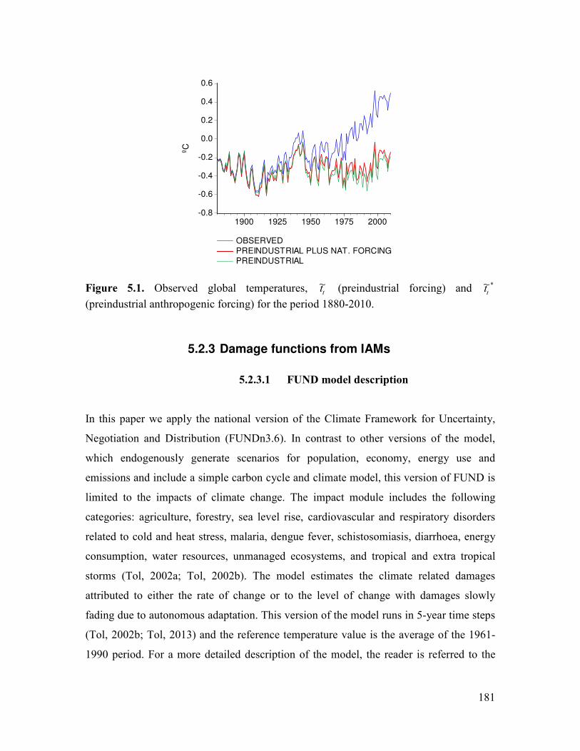
temperatures, respectively. These time series, depicted in Figure 5.1, provide alternative
climate scenarios for running the selected IAMs. The first scenario, tt~ from equation
(5.2), represents natural variability under a stationary climate where all external radiative
forcings are held constant at their preindustrial values (preindustrial scenario). The
second scenario, *~tt from equation (5.3), represents the evolution of global temperatures
holding the main anthropogenic forcing factors (GHG and RAER) constant at their
preindustrial values, but allowing all other forcing factors to vary according to the
observed records (natural forcing scenario). The third scenario, represented by equation
(5.1), corresponds to the observed temperature records.
181
-0.8
-0.6
-0.4
-0.2
0.0
0.2
0.4
0.6
1900 1925 1950 1975 2000
OBSERVED
PREINDUSTRIAL PLUS NAT. FORCINGPREINDUSTRIAL
ºC
Figure 5.1. Observed global temperatures, tt
~ (preindustrial forcing) and *~tt
(preindustrial anthropogenic forcing) for the period 1880-2010.
5.2.3 Damage functions from IAMs
5.2.3.1 FU�D model description
In this paper we apply the national version of the Climate Framework for Uncertainty,
Negotiation and Distribution (FUNDn3.6). In contrast to other versions of the model,
which endogenously generate scenarios for population, economy, energy use and
emissions and include a simple carbon cycle and climate model, this version of FUND is
limited to the impacts of climate change. The impact module includes the following
categories: agriculture, forestry, sea level rise, cardiovascular and respiratory disorders
related to cold and heat stress, malaria, dengue fever, schistosomiasis, diarrhoea, energy
consumption, water resources, unmanaged ecosystems, and tropical and extra tropical
storms (Tol, 2002a; Tol, 2002b). The model estimates the climate related damages
attributed to either the rate of change or to the level of change with damages slowly
fading due to autonomous adaptation. This version of the model runs in 5-year time steps
(Tol, 2002b; Tol, 2013) and the reference temperature value is the average of the 1961-
1990 period. For a more detailed description of the model, the reader is referred to the

182
original papers and technical documentation available at http://www.fund-model.org/; the
model code for this version is at http://dvn.iq.harvard.edu/dvn/dv/rtol.
5.2.3.2 The DICE damage function
The damage function of DICE was developed from estimates from 12 world regions and
includes damages to major sectors such as agriculture, the cost of sea-level rise, adverse
impacts on health, and nonmarket damages, as well as estimates of the potential costs of
catastrophic damages (Nordhaus, 2008). The aggregated impact function can be
described as follows:
2
21 ttt TTD θθ += (5.4)
where tD represents the climate damage as fraction of output, 1θ and
2θ are the
parameters of the damage function calibrated for the world, tT is global temperature
increase over its 1900 value. For this paper we consider the DICE99 (Nordhaus and
Boyer, 2000) and the DICE2007 (Nordhaus, 2008; Nordhaus, 2010). Parameterizations
are shown in Table C1. The main difference in the parameterization of DICE99 and
DICE2007 consists in that in the former the climate impacts for small temperature
increases were estimated to produce net positive benefits, while in the latter all
temperature increases lead to net negative impacts (Nordhaus, 2008). A one-year time
step was chosen for all estimates presented here.
5.2.3.3 The PAGE2002 damage function
The PAGE2002 model damage functions include the uncertainty in the functions'
coefficients by means of triangular distributions parameterized to cover the range of
possible impacts that have been reported in the literature. The main aim is to offer a
probabilistic representation of the potential climate change damages to inform decision-
making (Hope, 2006).

183
The impact functions of PAGE2002 can be expressed as follows:
,
, , , ,2.5
β
α∆
=
t r
t d r d r t r
TI Y (5.5)
, , ,γ π=t r t r t t rD Y (5.6)
where , ,t d rI represents the economic impacts in time t, in the sector d (d=1,2;
representing the economic and the noneconomic sectors, respectively) and in region r;
rtT ,∆ is the increment in regional temperature with respect to its preindustrial value (in
this case, its value in 1880); β is the exponent that determines the functional form of the
impact function; and ,α d r are regional parameters to express the percentage of GDP ( rtY , )
lost for a benchmark warming of 2.5°C in each impact sector and region. Equation (5.6)
represents the impacts associated to the occurrence of a large-scale discontinuity in the
climate system. ,t rD represents the economic impacts of a discontinuity at time t and
region r; ,γ t r is the economic impact of a discontinuity at time t in region r; and π is the
probability of occurrence of the discontinuity. The total economic impacts are the sum of
equations (5.5) and (5.6).
Given that the observed warming during the 20th century was below the lower limit for
the occurrence of large-scale discontinuities, the economic damages presented here come
from equation (5.5) only. The regional weights for scaling the impact functions are those
from the PAGE2002 model (reproduced in Table C2; see Hope, 2006) and the regional
estimates of temperature where produced using the scaling factors obtained from the
emulation of the UKMOHADCM3 General Circulation Model of the Magicc/Scengen
software (http://www.cgd.ucar.edu/cas/wigley/magicc/)13
. The outcomes of the damage
functions described above were estimated using simulation experiments of 1,000
realizations and the time-step was chosen to be one year. The global estimates of the
13
The regional scaling factors are: 1.56 for Europe; 1.39 for Latin America; 1.49 for North
America/OECD; 1.30 for Africa; 2.04 for North Asia; 1.33 for South Asia and; 1.45 for China.

184
climate damages during the 20th century presented here are simple averages of the
regional damage functions. The updated version PAGE2009 includes significant changes
in its climate, impacts, emissions and adaptation modules (Hope, 2011a,b). However, in
this study we focus on the PAGE2002 since it has been used in influential studies (e.g.,
Stern, 2006) and has been widely discussed in the literature. Besides, PAGE2009 cannot
be used without permission.
5.2.3.4 Damage function from recent literature
review
Based on a literature review of all published estimates of the global costs of climate
change, Tol (2009; 2014) estimates a damage function that synthesizes all findings. The
damage function takes the same functional form of equation (4), but the parameters
values are -0.251 =θ and -0.162 =θ . This damage function is calibrated with respect to
the preindustrial climate (in this case, global temperature in 1880). We will refer to this
impact function as MA (for meta-analysis).
5.3 Results and discussion
In this section we present estimates of the contributions of natural and anthropogenic
factors to the projected costs of observed global temperature during a period comprising
the 20th century. Based on the three temperature scenarios in section 2.2, five economic
impact scenarios are defined:
1. S_OBS: The expected economic costs given the observed global temperature
evolution, obtained using tT .
2. S_NV: The expected costs associated to natural variability under a stationary
climate holding all external forcing factors constant at their preindustrial levels,
obtained using tt~ .

185
3. S_NVF: The expected costs associated to the observed natural external forcing
and internal variability, obtained using *~tt . This scenario is used only for
estimating S_AF and S_NF described below.
4. S_AF: The expected costs associated to the anthropogenic radiative forcing,
obtained as the difference of S_OBS and S_NVF.
5. S_NF: The expected costs associated to the natural radiative forcing, obtained as
the difference of S_NVF and S_NV.
Note that this approach for separating the contributions of internal variability and
anthropogenic and natural forcing preserves their interaction effects (e.g., the effects of
natural variability under a stationary climate are not the same that under an externally
forced climate due to the nonlinearities in the damage functions).
5.3.1 Estimates of costs obtained from observed
global temperatures
Panel a) of Figure 5.2 shows the estimated impacts of the observed climate during the
20th century according to the 5 different IAMs. These models do not agree on the sign or
the magnitude of the estimated welfare impacts. Nevertheless, as in the case of global
temperature series, the costs obtained from the different IAMs show, in general, a slight
trend from the beginning of the sample until the mid-1970's when a large increase in their
rates of growth occurred. A slight deceleration since the mid-1990s is also noticeable,
which is in line with the recent slowdown in the rate of warming that has been reported
(Estrada et al., 2013b; Kaufmann et al., 2011). According to PAGE2002, MA and
DICE2007, by the end of the century the observed global temperature had a negative
effect on welfare. For DICE99 and FUNDn3.6 the effect was positive. While DICE99,
DICE2007, MA and PAGE2002 suggest that the economic impacts during the last decade
are small (about -0.26% to 0.14% of global GDP), FUNDn3.6 shows considerably larger
(positive) impacts reaching about 1% of GDP in 2000. FUNDn3.6 equity weighting

186
results show the highest benefits14
: 1.19% in 2000 and a maximum of 1.61% in the mid-
1970s. Note that the magnitude of the impacts over the last three decades is
unprecedented over the last century. Only in the case of DICE99 the impacts before the
anthropogenic intervention became significant are larger than those estimated for the end
of the 20th century.
a)
-0.4
0.0
0.4
0.8
1.2
1.6
1900 1920 1940 1960 1980 2000
PAGE2002 DICE2007 DICE99MA FUND average FUND equity
S_OBS
% G
DP
b)
-0.4
0.0
0.4
0.8
1.2
1.6
1900 1920 1940 1960 1980 2000
PAGE2002 DICE2007 DICE99MA FUND average FUND equity
S_AF
% G
DP
c)
-0.4
0.0
0.4
0.8
1.2
1.6
1900 1920 1940 1960 1980 2000
PAGE2002 DICE2007 DICE99MA FUND average FUND equity
% G
DP
S_NF
d)
-0.4
0.0
0.4
0.8
1.2
1.6
1900 1920 1940 1960 1980 2000
PAGE2002 DICE2007 DICE99MA FUND average FUND equity
S_NV
% G
DP
Figure 5.2. Estimated economic effects over the 20th century obtained from S_OBS
(panel a), S_AF (panel b), S_NF (panel c) and S_NV (panel d).
Figure 5.3 panel a) shows the multimodel mean of S_OBS and the corresponding two
standard deviation intervals representing the uncertainty in this estimate. For the
14
According to the FUND model during the 20th century the poorer countries experienced greater benefits,
primarily from CO2 fertilization, than the richer countries and therefore the equity weighted impacts are
more positive than the non-weighted average (see Tol, 2009).

187
estimates in Figure 5.3 all IAMs are weighted equally, implying that all of them produce
equally credible estimates. Although this is probably not the case, until now IAMs'
projections have not been validated and their performance is unknown. The multimodel
mean in Figure 5.3 panel a) shows a steady positive trend that leads to net benefits of
about 0.30% of GDP in 2000. Note however that throughout the 20th century, the
multimodel mean value is always smaller than the standard deviation of the models'
outcomes, underlying the very large uncertainty in these estimates (e.g., the standard
deviation in 2000 was 0.56%).
In the following subsections, the costs associated to observed climate variability and
change are decomposed into their natural and anthropogenic components.
a)
-1.5
-1.0
-0.5
0.0
0.5
1.0
1.5
2.0
1900 1920 1940 1960 1980 2000
S_OBS
% G
DP
b)
-1.5
-1.0
-0.5
0.0
0.5
1.0
1.5
2.0
1900 1920 1940 1960 1980 2000
S_AF
% G
DP
c)
-1.5
-1.0
-0.5
0.0
0.5
1.0
1.5
2.0
1900 1920 1940 1960 1980 2000
% G
DP
S_NF
d)
-1.5
-1.0
-0.5
0.0
0.5
1.0
1.5
2.0
1900 1920 1940 1960 1980 2000
S_NV
% G
DP
Figure 5.3. Multimodel mean of the estimated economic effects over the 20th century.
S_OBS (panel a), S_AF (panel b), S_NF (panel c) and S_NV (panel d).

188
5.3.2 Contributions of the natural and
anthropogenic radiative forcing to the
estimated impacts from the observed global
temperatures
Panels a), b) and c) of Figure 5.2 show that the trending behavior of the estimated global
economic impacts S_OBS can only be explained by S_AF and S_NF. As clearly shown
in panel d), the costs associated to natural variability describe oscillatory patterns around
a fixed mean that cannot account for the trend in global impacts (see Section 5.3.3 for an
analysis of the natural variability impacts).
S_AF (Figure 5.2b) describes quite closely the general nonlinear trend in S_OBS.
Although estimates of the different IAMs do not agree on the sign (nor on the magnitude)
of the effects of anthropogenic forcing, all of them describe the anthropogenic
contribution steadily increased over the first part of the century and rapidly accelerated
since the mid 1970's. They also show a deceleration during the first decade of the 21st
century, which is consistent with the reported slowdown in the warming during the last
two decades (e.g., Estrada et al., 2013b). Note that S_NF also shows a similar nonlinear
trend, but as described below, the effects of natural forcing at the end of the century are,
for most models, about one order of magnitude lower than those associated to
anthropogenic forcing (see Figure C1 for a comparison of natural and anthropogenic
contributions per model). Moreover, its impacts where practically zero until the late
1940s.
According to PAGE2002, MA, DICE99 and DICE2007, the welfare impacts of
anthropogenic forcing lie in the range of a few tenths of percent of the world GDP by the
end of the 20th century (from -0.23% in PAGE2002 to 0.24% in DICE99). This figure is
considerably larger for FUNDn3.6 which indicates benefits in the range of about 0.60%
to 1.37%. It is also worth noting that DICE2007 provides the smallest estimates of
impacts, reaching only about -0.1% at the end of the century.

189
The multimodel mean of S_AF indicates that the human contribution to the observed
warming during the 20th century produced net benefits in the world average. The benefits
increased from about 0.08% at the beginning of the century to about 0.19% of GDP in
2000 after reaching about 0.33% in the 1990's (Figure 5.3 panel b). As before, the
uncertainty is quite large: the multimodel mean is always smaller than the standard
deviation of the models' outcomes.
The contribution of S_NF to the overall impacts is depicted in panel c) of Figure 5.2. The
effects of natural forcing are dominated by the eleven-year cycle in solar forcing. The
correlation between the impacts attributed to natural forcing factors with solar forcing is
very large and positive for DICE99, DICE2007, MA and FUNDn3.6 ranging from 0.62
to 0.91, while for PAGE2002 is -0.84. Note that in all cases except DICE2007, the
increases in natural forcing observed since the mid-20th century make S_NF contribute in
the same direction as S_AF to the estimated total costs. This is expected from climate
physics: irrespective of their origin, increases in radiative forcing simply add up, leading
to larger climate transient response and equilibrium temperatures (Schwartz, 2012). Thus,
increases in radiative forcing from natural and anthropogenic origin should not produce
opposite effects (trends), but reinforce the impacts in the same direction instead.
The multimodel mean shows that the impacts of S_NF where practically zero until the
1940s. In the second half of the century natural forcing (mainly solar) produced small but
increasing benefits reaching around 0.04% of GDP in 2000. When the magnitude of the
anthropogenic contribution is compared to the other sources of impacts, it can be argued
that at the end of the 20th century human activities became dominant drivers of the
estimated economic impacts, producing similar or larger impacts than those of low-
frequency natural variability.

190
5.3.3 Estimates of costs obtained from the
preindustrial radiative forcing scenario
All of the impact functions indicate that the natural variability alone can lead to impacts
that are comparable in magnitude to those that can be attributed to anthropogenic factors
until the last three decades of the 20th century and are much larger than those that can be
associated to the observed natural forcing (Figure 5.2d). The main difference is that the
natural variability impacts follow low-frequency oscillations instead of sustained trends.
Only in the case of DICE2007 the impacts of natural variability are strictly negative,
while for DICE99 are mostly negative and for PAGE2002 and MA they are mainly
positive. These non-monotonic impacts are dominated by the low-frequency variability
and large persistence of the climate system.
The impacts under the preindustrial scenario can be associated with some of the main
modes of interannual climate variability. As shown in Table C3, S_NV is highly and
significantly correlated with AMO and to a lesser extent with SOI, PDO and NAO. The
magnitude of these correlations is broadly similar for the estimates obtained using the
PAGE2002, MA, DICE99 and DICE2007 impact functions (about 0.70, 0.30, 0.20 and
0.24 in absolute value for AMO, SOI, PDO and NAO, respectively) although the signs
are different depending on the specification of the impact functions. In the case of
FUNDn3.6, the correlation coefficients between these climate modes and S_NV are
generally lower in magnitude and not statistically significant (with the exception of AMO
and FUNDn3.6 equity), probably due to the 5 year time-step of this model, the limited
number of observations available for estimating these quantities (22 data points) and
possibly to the model structure, as discussed below.
Linear regression models using AMO, SOI, PDO and NAO as explanatory variables were
estimated but only the first two (AMO and SOI) were found to significantly contribute to
explain the variability of the estimated costs. The following specification was found to be

191
statistically adequate for most of the IAMs projections15
(see Tables C4 and C5 for
parameter estimates and misspecification tests):
ttttitit SOIAMOAMO>VSc>VS εγδδα +++++= −− 1211__ (5.7)
where it>VS _ are the estimated costs for model 5,...,1=i . This regression model has a
similar specification to those in Estrada et al. (2013b) and Estrada and Perron (2012) for
global temperature series. In all cases AMO and SOI are highly significant, except for the
estimates obtained with FUNDn3.6 where only AMO is significant. This result probably
has to do with the limited number of observations (and time-step) in the projections
obtained with FUNDn3.6 and more importantly, with the large differences in the
structure and complexity of FUNDn3.6 compared to the other IAMs. The impact
functions of PAGE2002, DICE99, DICE2007 are simple power functions of temperature,
and results thus preserve strong similarities with the characteristics of global
temperatures. However, this is not the case of FUNDn3.6 as its impact functions
significantly modify the characteristics of the input temperature series.
For most IAMs, the estimated regressions explain about 60% of the variance of the
impacts associated to natural variability. Furthermore, AMO and SOI generate important
fluctuations from the mean of it>VS _ : a one standard deviation shock to AMO produces
a cumulative long-run response of about 0.60 times the standard deviation of it>VS _
(positive for DICE99 and DICE2007, negative for PAGE2002 and MA) while a shock of
one standard deviation to SOI generates a long-term response 0.45 times the standard
deviation of it>VS _ (negative for DICE99 and DICE2007, the opposite occurs with
PAGE2002. See Table C6). For FUNDn3.6 a one standard deviation shock in AMO
produces a response of 0.39 (average) and 0.77 (equity) times the standard deviation of
it>VS _ .
15
Most of the regression models are statistically adequate according to the misspecification tests that were
applied. Only in the case of DICE2007 and FUNDn3.6 average deviations from the normality assumption
were found. In addition, the CUSUMQ test suggests some evidence of parameter instability for FUNDn3.6.
In the case of MA, SOI was omitted due to functional form problems.
192
The multimodel mean of S_NV is mainly negative and shows a low-frequency oscillatory
pattern similar to AMO (correlation coefficient of 0.60) varying in a range of -0.08% to
0.17% of GDP during the 20th century. The multimodel mean of S_NV suggest that until
the last three decades of the 20th century, natural variability was the main source of
economic impacts. Since then, the main driver of impacts is anthropogenic forcing. It is
worth noticing that the standard deviation of the models' outcome is in average almost 3
times larger than the multimodel mean, indicating the large uncertainty in this estimate.
5.4 The anthropogenic and natural components of the estimated impacts per sector.
As mentioned above, FUNDn3.6 allows us to investigate the projected impacts separately
for each sector. Figure 5.4 shows the anthropogenic and natural contributions to the
economic costs of observed 20th century climate for agriculture, health, water resources,
and energy.
Agriculture is the sector for which the observed climate had the largest effect, leading to
benefits of about 0.8% of GDP in 2000 (Figure 5.4 panel a). This sector is by far where
the anthropogenic influence is more evident, leading at the end of the 20th century to
gains of 0.68% of GDP. This is the only sector for which the anthropogenic contribution
is considerably larger than the effects of natural variability. Carbon dioxide fertilization
contributes most to these gains. The effects of natural forcing became positive around the
1930's and reached 0.06% in 2000, about one order of magnitude lower than the
estimates of the anthropogenic contribution. For this sector, natural variability produced
fluctuations in the range of about -0.15% to 0.06% of GDP, substantially larger than the
contribution of natural forcing.

193
a)
-0.2
0
0.2
0.4
0.6
0.8
1
1895
1900
1905
1910
1915
1920
1925
1930
1935
1940
1945
1950
1955
1960
1965
1970
1975
1980
1985
1990
1995
2000
%G
DP
S_OBS
S_NV
S_AF
S_NF
b)
-0.4
-0.3
-0.2
-0.1
0
0.1
0.2
0.3
1895
1900
1905
1910
1915
1920
1925
1930
1935
1940
1945
1950
1955
1960
1965
1970
1975
1980
1985
1990
1995
2000
% G
DP
S_OBS
S_NV
S_AF
S_NF
c)
-0.3
-0.2
-0.1
0
0.1
0.2
0.3
0.4
0.5
1895
1900
1905
1910
1915
1920
1925
1930
1935
1940
1945
1950
1955
1960
1965
1970
1975
1980
1985
1990
1995
2000
% G
DP
S_OBS
S_NV
S_AF
S_NF
d)
-0.5
-0.4
-0.3
-0.2
-0.1
0
0.1
0.2
0.3
0.4
0.5
1895
1900
1905
1910
1915
1920
1925
1930
1935
1940
1945
1950
1955
1960
1965
1970
1975
1980
1985
1990
1995
2000
% G
DP
S_OBS
S_NV
S_AF
S_NF
Figure 5.4. Estimated economic effects over the 20th century per sector: panel a)
agriculture, panel b) water resources, panel c) energy and panel d) health.
In the water resources sector, both anthropogenic and natural forcing imparted a trend on
losses (Figure 5.4 panel b). The anthropogenic contribution led to losses of up to -0.12%
of GDP and, in the last decades of the past century, it became about five times larger than
the effects of natural forcing. However, the amplitude of the costs produced by low-
frequency natural variability is considerably larger compared to the individual or joint
contributions of natural and anthropogenic factors.
Low-frequency natural variability plays a dominant role on the costs of the two
remaining sectors (Figure 5.4 panels c and d). The interaction effects between natural
variability and forcing factors are large and add significant noise to the anthropogenic
and natural forcings signals. In the energy sector benefits from the observed global
temperature of about 0.36% were attained in 2000 (Figure 5.4 panel c). The
anthropogenic forcing contributed to these gains during the whole 20th century reaching
up to 0.20% in the 1990s. In comparison, the positive effects of natural forcing started

194
around the 1930s and due to the interaction effects, the benefits from natural forcing
reached 0.34% in 1990. In 1995, the anthropogenic and natural contributions generated
gains of about 0.17% and 24%, respectively, and then dropped considerably. Although in
all sectors the effects of the slowdown in the warming can be detected, in the energy
sector this is more evident due to the large interaction effects of forcing factors and
natural variability. In 2000 the benefits of anthropogenic and natural forcing amounted to
only 0.02% and 0.08%, respectively.
In the health sector, the negative impacts of the 20th century climate reached about 0.2%
of GDP in 2000 (Figure 5.4 panel d). Although the contribution of anthropogenic forcing
was negative during most of the century it was not until the 1970s that a negative trend
became noticeable. For this sector, both anthropogenic and natural contributions to the
costs of the 20th century climate are well within the amplitude of the effects of natural
variability.
Nevertheless, as shown in Figure 5.5, the anthropogenic contribution to the estimated
number of deaths per million people related to climate is dominant (panel b). As shown in
panels a) and b) of Figure 5.5, the trend in the estimated number of deaths of these of
climate related diseases is mainly imparted by the anthropogenic forcing. The largest
contribution of anthropogenic forcing to these numbers occurs in diarrhoea, respiratory
diseases and malaria. Natural forcing (panel c) and internal variability (panel d) mainly
provided the low-frequency oscillatory pattern shown by the proportion of deaths.

195
a)
b)
c)
d)
Figure 5.5. Estimated deaths per million people during the 20th century per disease
obtained from S_OBS (panel a), S_AF (panel b), S_NF (panel c) and S_NV (panel d).
5.5 Discussion and conclusion
The decomposition of the estimated impacts of observed global temperature reveals a
clear anthropogenic influence that at the end of the century becomes even larger in
magnitude than the impacts of natural variability. Anthropogenic impacts increased over
the period of analysis in a non monotonic way, slowly for the first part of the 20th
century, accelerating significantly after the 1970s and reducing their rate of increase after
the 1990s when a slowdown in global warming started (Gay-Garcia et al., 2009; Estrada
et al., 2013b). As expected, natural forcing is shown to reinforce the impacts attributed to
anthropogenic forcing. The contribution of natural forcing to the total estimated impacts
is about one order of magnitude lower than that of the anthropogenic forcing or that of

196
the internal interannual variability. The main driver of the impacts associated to natural
factors is solar forcing, which imprinted its 11-year cycle and a slight positive trend.
In the intra- and inter-decadal scales the amplitude of the impacts associated to natural
variability is considerably larger than that produced by anthropogenic factors during the
first half of the century. These non monotonic impacts are mostly determined by the low-
frequency variability modes and persistence of the climate system.
IAMs do not agree in the sign nor the magnitude of the impacts for small changes in
temperature. In the case of FUNDn3.6 and DICE99 the observed warming has brought
benefits to the global GDP, while according to DICE2007, MA and PAGE2002 the
opposite is true. With the exception of FUNDn3.6, which estimates the magnitude of the
impacts in about 1% of GDP at the end of the 20th century, the rest of the IAMs
considered value the impacts in only a few tenths of percent.
According to the sectoral decomposition of the estimated impacts obtained by
FUNDn3.6, the effects of anthropogenic forcing in agriculture account for most of the
economic benefit in the past century. Benefits attributable to the anthropogenic forcing
are also found for the energy sector, while this forcing imparted a trend to economic
losses in human health and water resources. The model strongly suggests that the
contribution of anthropogenic forcing to the estimated number of deaths per thousand
people is dominant in the case of diarrhoea, respiratory diseases and malaria.
This chapter adds to the recent discussion regarding IAMs by illustrating the large
differences in the projections obtained from model to model for small increases in
temperatures. This is related to the problem of model validation which could help to
improve the specification and calibration of the impact functions in IAMs, to reduce the
large uncertainty characterizing these models, and to increase their credibility. However,
while the assessment of the performance of other types of models (e.g., general
circulation models) is straightforward due to the existence of readily available observed
datasets covering long periods of time and with high spatial resolution (e.g., temperature

197
and precipitation), this is not the case of the welfare impacts of observed climate. Until
now the performance of the different IAMs has not been assessed and the validity of their
projections thus remains unknown. The current lack of proper validation methods and of
research efforts devoted to develop them constitutes a significant challenge for the
advancement of integrated assessment models.

198
Appendix C
a)
-0.28
-0.24
-0.20
-0.16
-0.12
-0.08
-0.04
0.00
0.04
0.08
0.12
1880
1900
1920
1940
1960
1980
2000
PAGE_OBS PAGE_AFPAGE_NF PAGE_NV
% G
DP
PAGE2002
b)
-0.30
-0.20
-0.10
0.00
0.10
0.20
0.30
1880
1900
1920
1940
1960
1980
2000
S_OBS S_AFS_NF S_NV
% G
DP
DICE99
c)
-0.15
-0.13
-0.10
-0.08
-0.05
-0.03
0.00
0.02
0.05
1880
1900
1920
1940
1960
1980
2000
S_OBS S_AFS_NF S_NV
% G
DP
DICE2007
d)
-0.25
-0.20
-0.15
-0.10
-0.05
0.00
0.05
0.10
1880
1900
1920
1940
1960
1980
2000
S_OBS S_AFS_NF S_NV
% G
DP
MA
e)
-0.4
-0.2
0.0
0.2
0.4
0.6
0.8
1.0
1900 1920 1940 1960 1980 2000
S_OBS S_AFS_NF S_NV
% G
DP
FUNDn3.6 average
f)
-0.4
0.0
0.4
0.8
1.2
1.6
2.0
1900 1920 1940 1960 1980 2000
S_OBS S_AFS_NF S_NV
% G
DP
FUNDn3.6 equity
Figure C1. Estimated economic effects for the 20th century per IAM. Panel a)
PAGE2002, panel b) DICE99, panel c) DICE2007, panel d) MA, panel e) FUNDn3.6
average and panel f) FUNDn3.6 equity.

199
Table C1. Parameter values of the damage functions in the DICE99 and DICE2007
models.
Model 1θ
2θ
DICE99 -0.00450 0.00350
DICE2007 0.00000 0.00284
Table C2. Parameter values for the economic and non-economic sectors for EU and
regional weights from PAGE2002.
Mean Min Mode Max
Economic impact in EU (%GDP for 2.5°C) 0.5 -0.1 0.6 1
Non-economic impact EU (%GDP for 2.5°C) 0.73 0 0.7 1.5
Impact function exponent 1.76 1 1.3 3
Eastern Europe & FSU weights factor -0.35 -1 -0.25 0.2
USA weights factor 0.25 0 0.25 0.5
China weights factor 0.2 0 0.1 0.5
India weights factor 2.5 1.5 2 4
Africa weights factor 1.83 1 1.5 3
Latin America weights factor 1.83 1 1.5 3
Other OECD weights factor 0.25 0 0.25 0.5
Table C3. Correlation coefficients between the estimated impacts from the preindustrial
scenario and AMO, SOI, NAO and PDO.
DICE99 DICE2007 MA PAGE2002 FUND
average
FUND
equity
AMO 0.70
(0.000)
-0.65
(0.000)
-0.70
(0.000)
-0.68
(0.000)
0.38
(0.097)
0.77
(0.000)
NAO -0.24
(0.012)
0.23
(0.017)
0.24
(0.012)
0.24
(0.011)
0.16
(0.506)
-0.19
(0.428)
SOI -0.30
(0.002)
0.31
(0.001)
0.28
(0.004)
0.31
(0.001)
0.18
(0.452)
0.10
(0.673)
PDO 0.21
(0.025)
-0.18
(0.061)
-0.23
(0.015)
-0.20
(0.032)
-0.05
(0.829)
-0.06
(0.817) P-values in parenthesis.

200
Table C4. Regression models for it>VS _ based on key variability modes and the
persistence of impacts.
it>VS _ c α 1δ 2δ γ 2R
DICE99 -0.0638
(-7.41)
0.4147
(5.55)
0.2500
(8.27)
-0.1041
(-2.92)
-0.0174
(-4.75)
0.65
DICE2007 -0.0099
(-7.06)
0.3632
(4.66)
0.0463
(6.87)
-0.0169
(-2.24)
-0.0374
(-4.61)
0.58
MA 0.0211
(-6.34)
0.4721
(6.04)
-0.0915
(-9.34)
0.0518
(4.46)
-- 0.62
PAGE2002 0.0160
(6.79)
0.3941
(5.21)
-0.0925
(-7.83)
0.0387
(2.85)
0.0070
(4.88)
0.63
FUND
average
0.0311
(1.01)
-- 0.3917
(1.89)
-- -- 0.15
FUND
equity
0.1595
(3.91)
-- 1.4678
(5.35)
-- -- 0.59
Bold and italic figures indicate statistical significance at the 5% and 10 levels. t-statistics are given in
parenthesis.

201
Table C5. Misspecification testing for the models for it>VS _ based on key variability
modes and the persistence of impacts. Misspecification test DICE99 DICE2007 PAGE2002 MA FUND average FUND equity
RESET
(F-statistic)
1 0.399
(0.529)
1.887
(0.062)
0.149
(0.700)
1.498
(0.137)
0.545
(0.469)
1.028
(0.317)
2 0.218
(0.805)
2.355
(0.099)
0.077
(0.926)
1.114
(0.332)
0.311
(0.737)
1.096
(0.355)
3 0.245
(0.865)
2.123
(0.101)
0.078
(0.972)
1.041
(0.377)
0.241
(0.866)
0.692
(0.569)
4 0.590
(0.670)
2.117
(0.083)
0.911
(0.460)
1.003
(0.409)
0.401
(0.805)
0.602
(0.667)
Jarque-Bera
1.064
(0.588)
6.654
(0.036)
2.904
(0.234)
1.483
(0.476)
9.54
(0.009)
0.509
(0.775)
Ljung-Box
(Q-statistic)
1 0.094
(0.759)
0.023
(0.879)
0.016
(0.900)
0.123
(0.726)
0.523
(0.470)
2.564
(0.109)
2 1.813
(0.404)
3.877
(0.144)
3.122
(0.210)
0.504
(0.777)
2.809
(0.246)
4.595
(0.101)
3 1.825
(0.609)
3.928
(0.269)
3.140
(0.371)
0.829
(0.843)
5.270
(0.153)
6.151
(0.104)
4 7.631
(0.106)
8.099
(0.088)
8.539
(0.074)
3.876
(0.423)
5.324
(0.256)
6.152
(0.188)
White (F-statistic)
1.252
(0.249)
1.620
(0.084)
1.580
(0.095)
1.230
(0.283)
0.724
(0.498)
0.442
(0.649)
McLeod-Li
1 0.064
(0.800)
2.857
(0.091)
1.080
(0.299)
1.404
(0.236)
0.359
(0.549)
0.889
(0.346)
2 0.193
(0.908)
4.408
(0.110)
1.334
(0.513)
1.520
(0.468)
2.530
(0.282)
2.180
(0.336)
3 0.224
(0.974)
7.485
(0.058)
2.430
(0.488)
1.698
(0.637)
2.610
(0.456)
2.569
(0.463)
4 0.708
(0.950)
7.743
(0.101)
2.664
(0.616)
1.741
(0.783)
3.099
(0.541)
3.238
(0.519)
Breusch-Godfrey
(F-statistic)
1 0.277
(0.599)
0.081
(0.777)
0.048
(0.827)
0.525
(0.470)
0.417
(0.526)
2.184
(0.156)
2 2.161
(0.120)
2.564
(0.081)
2.730
(0.069)
0.281
(0.756)
1.299
(0.297)
3.288
(0.061)
3 1.481
(0.223)
1.700
(0.171)
1.834
(0.145)
0.299
(0.826)
1.230
(0.330)
2.071
(0.142)
4 2.363
(0.057)
1.901
(0.115)
2.328
(0.060)
1.041
(0.389)
0.880
(0.498)
1.492
(0.251)
ARCH
(F-statistic)
1 0.062
(0.804)
2.803
(0.097)
1.046
(0.309)
1.360
(0.246)
0.278
(0.605)
0.713
(0.409)
2 0.091
(0.913)
1.861
(0.160)
0.582
(0.560)
0.800
(0.451)
0.864
(0.439)
0.679
(0.520)
3 0.082
(0.970)
1.907
(0.132)
0.668
(0.574)
0.590
(0.623)
0.502
(0.686)
0.433
(0.732)
4 0.174
(0.951)
1.637
(0.169)
0.569
(0.686)
0.434
(0.784)
0.536
(0.712)
0.581
(0.682)
CUSUM Stability Stability Stability Stability Stability Stability
CUSUMQ Stability Stability Stability Stability Instability Stability
Bold figures indicate statistical significance at the 5% level. P-values are given in parenthesis.

202
Table C6. Long-run response of estimated impacts to one standard deviation shocks to
AMO and SOI as a percentage of GDP.
DICE99 DICE2007 MA PAGE2002 FUND
average
FUND
equity
AMO 0.046
[0.635]
-0.009
[-0.587]
-0.014
[-0.598]
-0.017
[-0.602]
0.058
[0.390]
0.216
[0.767]
SOI -0.033
[-0.451]
0.007
[0.444]
-- 0.014
[0.470]
-- --
Numbers in brackets represent the response of the estimated impacts as a fraction of their standard
deviation.