5. ACSC performance under windy conditions

i

A numerical investigation of air-cooled steam condenser

performance under windy conditions

by

Michael Trevor Foxwell Owen

March 2010

Thesis presented in partial fulfilment of the requirements for the degree

Master of Science in Engineering at the University of Stellenbosch

Supervisor: Prof. Detlev Kröger

Department of Mechanical and Mechatronic Engineering

i

Declaration

By submitting this thesis electronically, I declare that the entirety of the work contained

therein is my own, original work, that I am the owner of the copyright thereof (unless to the

extent explicitly otherwise stated) and that I have not previously in its entirety or in part

submitted it for obtaining any qualification.

Date: 10 February 2010

Copyright © 2010 Stellenbosch University All rights reserved

Stellenbosch University http://scholar.sun.ac.za

ii

Abstract

This study is aimed at the development of an efficient and reliable method of evaluating the

performance of an air-cooled steam condenser (ACSC) under windy conditions, using

computational fluid dynamics (CFD). A two-step modelling approach is employed as a result

of computational limitations. The numerical ACSC model developed in this study makes use

of the pressure jump fan model, amongst other approximations, in an attempt to minimize the

computational expense of the performance evaluation. The accuracy of the numerical model

is verified through a comparison of the numerical results to test data collected during full

scale tests carried out on an operational ACSC. Good correlation is achieved between the

numerical results and test data. Further verification is carried out through a comparison to

previous numerical work. Satisfactory convergence is achieved for the most part and the few

discrepancies in the results are explained. The effect of wind on ACSC performance at El

Dorado Power Plant (Nevada, USA) is investigated and it is found that reduced fan

performance due to distorted flow at the inlet of the upstream fans is the primary contributor

to the reduction in performance associated with increased wind speed in this case. An attempt

is subsequently made to identify effective wind effect mitigation measures. To this end the

effects of wind screens, solid walkways and increasing the fan power are investigated. It is

found that the installation of an appropriate wind screen configuration provides a useful

means of reducing the negative effects of wind on ACSC performance and an improved wind

screen configuration is suggested for El Dorado. Solid walkways are also shown to be

beneficial to ACSC performance under windy conditions. It is further found that ACSC

performance increases with walkway width but that the installation of excessively wide

walkways is not justifiable. Finally, increasing the fan power during periods of unfavourable

ambient conditions is shown to have limited benefit in this case. The model developed in this

study has the potential to allow for the evaluation of large ACSC installations and provides a

reliable platform from which further investigations into improving ACSC performance under

windy conditions can be carried out.


iii

Opsomming

Hierdie studie is daarop gemik om die ontwikkeling van 'n geskikte en betroubare metode

van evaluering van die verrigting van ’n lugverkoelde stoom-kondensator (air-cooled steam

condenser, ACSC) onder winderige toestande, met behulp van numeriese vloei-dinamika. ’n

Twee-stap modelleringsbenadering is aangewend as gevolg van rekenaar beperkings. Die

numeriese ACSC-model wat in hierdie studie ontwikkel is, maak gebruik van die druksprong

waaier model, asook ander benaderings, in ’n poging om die berekeningskoste van die

verrigting-evaluering te verminder. Die akkuraatheid van die numeriese model is bevestig

deur middel van ’n vergelyking van die numeriese resultate met toetsdata ingesamel tydens

die volskaal toetse uitgevoer op ’n operasionele ACSC. Goeie korrelasie is bereik tussen die

numeriese resultate en toetsdata. Verdere bevestiging is uitgevoer deur middel van ’n

vergelyking met vorige numeriese werk. Bevredigende konvergensie is in die algemeen

bereik en die paar verskille in die resultate word verduidelik. Die effek van wind op ACSC

verrigting by El Dorado Power Plant (Nevada, VSA) is ondersoek, en daar is bevind dat

verlaagde waaierverrigting, as gevolg van vervormde vloei by die inlaat van die stroomop

waaiers, die primêre bydraer is tot die afname in ACSC werkverrigting geassosieer met

verhoogde windsnelheid in hierdie geval. ’n Poging word dan aangewend om effektiewe

wind-effek velagingsmaatreëls te identifiseer. Windskerms, soliede wandelvlakke en die

verhoging van die waaierkrag word gevolglik ondersoek. Daar is bevind dat die installasie

van ’n toepaslike windskerm-opset ’n nuttige middel tot ’n vermindering van die negatiewe

effekte van wind op ACSC verrigting bied, en ’n verbeterde windskerm opset is voorgestel

vir El Dorado. Soliede wandelvlakke word ook aanbeveel as voordelig vir ACSC verrigting

onder winderige toestande. Dit is verder bevind dat die ACSC prestasie verhoog met

wandelvlak breedte, maar dat die installasie van ’n te ruim wandelvlak nie regverdigbaar is

nie. Ten slotte, word bewys dat die verhoging van die waaierkrag tydens periodes van

ongunstige omgewingsomstandighede ’n beperkte voordeel in hierdie geval het. Die model

wat ontwikkel is in hierdie studie het die potensiaal om voorsiening te maak vir die

evaluering van groot ACSC- installasies en bied ’n betroubare platform vanwaar verdere

ondersoeke tot die verbetering van ACSC verrigting onder winderige toestande uitgevoer kan

word.


iv

Acknowledgements

I would like to express my sincerest gratitude to the following people/organizations for their

contribution towards making this study possible:

• Prof. D.G. Kröger for his support, knowledge and guidance.

• My family for their support and encouragement.

• Dr. J Maulbetsch for his generosity, hospitality and assistance.

• Mrs. F. Allwright and Mrs. S. van der Spuy for their willingness to assist.

• Mr. S.J. van der Spuy and Mr. H.C. Reuter for their help and enthusiasm.

• The California Energy Commission and the National Research Foundation for their

financial support.


v

Table of contents

Page

Declaration ………………………………………………………………………. i

Abstract ………………………………………………………………………….. ii

Opsomming ……………………………………………………………………...... iii

Acknowledgements ……………………………………………………………… iv

List of figures ........................................................................................................ viii

List of tables …………………………………………………………………… xiii

Nomenclature …………………………………………………………………… xiv

1. Introduction …………………………………………………………….... 1

1.1 Background and motivation ………………………………………... 1

1.2 Literature study …………………………………………………….. 4

1.3 Problem statement and objectives ………………………………… 8

2. System description ………………………………………………………... 9

2.1 System components ……………………………………………….... 9

2.1.1 Finned tube heat exchanger ………………………………. 10

2.1.2 Axial flow fan …………………………………………….... 11

2.2 Thermal-flow analysis …………………………………………….... 11

2.2.1 Energy equation …………………………………………... 12

2.2.2 Draft equation …………………………………………... 13

3. Numerical modelling ………………………………………………………. 14

3.1 CFD code overview ……………………………………………….... 14

3.1.1 Governing equations ………………………………………. 14

3.1.2 Discretization ………………………………………. 15

3.1.3 Turbulence model ………………………………………. 17

3.1.4 Buoyancy effects ………………………………………. 18

3.1.5 Boundary and continuum conditions ……………………... 19

3.2 Numerical ACSC model ……………………………………………. 20

3.2.1 Global flow field ……………………………………. 21


vi

3.2.2 Detailed ACSC model …………………………………… 24

3.2.3 Ideal flow model …………………………………… 29

3.3 Performance measures ……………………………………………... 30

4. Evaluation of the numerical models ………………………………………. 33

4.1 Sensitivity analysis ……………………………………………….... 33

4.1.1 Grid resolution …………………………………………… 33

4.1.2 Boundary proximity ………………………………………. 35

4.1.3 Global-to-detailed ACSC model iteration frequency …..….. 37

4.2 Evaluation of the numerical model through a comparison to

test data …………………………………………………………….... 38

4.2.1 Turbine operation under ideal conditions ……………….... 38

4.2.2 Test operating points ………………………………………. 39

4.2.3 Comparison of numerical results to test data …………….. 40


previous numerical work …………………………………………...... 41

5. ACSC performance under windy conditions ……………………………... 43

5.1 Reduced fan performance due to distorted inlet conditions ..……. 45

5.2 Hot plume recirculation …………………………………………… 47

5.3 Identification of the primary cause of ACSC performance

reduction under windy conditions …………………………………… 48

6. Evaluation of wind effect mitigation measures …………………..……….. 50

6.1 Wind screens …………………………………………………….... 50

6.1.1 Evaluation of the current wind screen configuration

at El Dorado ………………………………………………… 50

6.1.2 Evaluation of alternative wind screen configurations ……….. 52

6.2 Walkways …………………………………………………………... 56

6.3 Increasing fan power ……………………………………………...... 58

7. Conclusion ………………………………………………………………...... 63

7.1 The development of an accurate and efficient numerical

ACSC model ………………………………………………………... 63


vii

7.2 ACSC performance under windy conditions ………………………. 64

7.3 Evaluation of wind effect mitigation measures ………………….... 65

7.3.1 Wind screens ……………………………………………... 65

7.3.2 Walkways ………………………………………………….. 66

7.3.3 Increasing fan power ……………………………………... 67

7.4 Importance of this study …………………………………………..... 67

References ……………………………………………………………………... 69

Appendix A - System specifications ……………………………………. 73

A.1 Finned tube heat exchanger… ………………………………………... 73

A.2 Axial flow fan ………………………………………………………... 74

Appendix B - Supplementary results ……………………………….. 76

B.1 A-frame vs. simple heat exchanger model …..……………………….. 76

B.2 Verification of the pressure jump fan and heat exchanger models ....... 77

Appendix C - Derivation of the fan performance characteristic for

the pressure jump fan model ……………………………........ 78

Appendix D - System loss coefficients ……………………………………. 80

D.1 Definition of losses in an ACSC system ............................................... 80

D.2 Evaluation of the loss coefficients for the generic ACSC ………….... 82

Appendix E - Derivation of the viscous and inertial loss coefficients ........... 85

Appendix F - Derivation of the heat exchanger energy source term ............. 87

Appendix G - Test operating periods ……………………………………… 89

G.1 Test period 1 (TP1) …………………………………………………... 91

G.2 Test period 2 (TP2) ………………………………………………….. 93

G.3 Test period 3 (TP3) ………………………………………………….. 95

G.4 Test period 4 (TP4) ………………………………………………….. 97

G.5 Power law profiles for wind and temperature data ............................. 99

Appendix H - Wind screen material tests ...................................................... 100


viii

List of Figures

Page

Figure 1.1 Combined cycle power plant schematic ……………………….. 1

Figure 1.2 Mechanical draft ACSC fan unit, (a) Schematic, (b) During

installation ………….…………………........................................ 3

Figure 1.3 Typical fan inlet flow distortions caused by (a) wind effects,

(b) the proximity of buildings, and (c) cross-draft induced

by other fans …………………………………………………….. 6

Figure 1.4 ACSC fan unit configuration, (a) El Dorado, (b) Generic ACSC ... 8

Figure 2.1 Schematic of a typical ACSC fan unit ………………………… 9

Figure 2.2 Finned tube heat exchanger (a) Typical elliptical finned tube,

(b) Two tube row configuration ……………………………….... 10

Figure 2.3 Finned tube heat exchanger arrangement ……………………… 11

Figure 3.1 Schematic of an ACSC, (a) Side elevation, (b) Side elevation

(simplified for global flow field model) ………………………… 21

Figure 3.2 Global flow field model ……………………………………….. 22

Figure 3.3 Section view (B-B) of the global flow field computational grid

(a) Expanded view illustrating mesh expansion in non-critical

areas, (b) Close-up view of the mesh in the region of interest ….. 23

Figure 3.4 Detailed ACSC model schematic ……………………………… 24

Figure 3.5 ACSC fan unit, (a) Numerical model, (b) Numerical model

dimensions ……..………………………………………………... 25

Figure 3.6 Computational grid in the region of each ACSC fan unit ……… 25

Figure 3.7 ACSC fan unit models, (a) Simplified version,

(b) A-frame version ……………………………………………... 26

Figure 3.8 Fan performance characteristics, (a) El Dorado, (b) Generic

ACSC ……………………………………………………………. 27

Figure 3.9 Ideal flow model schematic ...................................................... 29

Figure 3.10 Ideal flow model computational mesh ………………………… 29


ix

Figure 4.1 Fan numbering scheme, (a) El Dorado, (b) Generic ACSC …… 33

Figure 4.2 The effect of grid resolution on the predicted volumetric

effectiveness of certain ACSC fans ……………………………... 34

Figure 4.3 Boundary proximity cases …………………………………….. 36

Figure 4.4 The effect of profile boundary proximity on the predicted

volumetric effectiveness of certain ACSC fans ..………...…….... 36

Figure 4.5 The effect of global-to-detailed ACSC model iteration frequency

on the predicted volumetric effectiveness of certain ACSC fans .... 37

Figure 4.6 Turbine performance under ideal conditions ………………….. 38

Figure 4.7 Comparison of numerically predicted and measured steam

turbine backpressure ……...……………………………………... 40

Figure 4.8 Comparison of the numerically predicted volumetric

effectivenesses of fans in (a) the upstream fan row, and (b) non-

upstream fan rows, under straight-flow wind conditions ……….. 41

Figure 4.9 Comparison of the numerically predicted ACSC thermal

effectiveness ……………………………………………………. 42

Figure 5.1 Effect of ambient conditions on ACSC heat transfer effectiveness

under (a) straight-flow, and (b) cross-flow wind conditions ….... 43

Figure 5.2 Effect of ambient conditions on steam turbine backpressure

under (a) straight-flow, and (b) cross-flow wind conditions …… 44

Figure 5.3 Fan volumetric effectiveness under straight-flow wind

conditions ……………………………………………………….. 45

Figure 5.4 Reason for the reduced performance of the windward fans:

(a) Static pressure (ps, N/m2), and (b) Vector plot (v, m/s) on

a section through the centre of fan (1,1) for a straight-flow wind

speed of vw = 9m/s ....................................................................…. 46

Figure 5.5 Static pressure (ps, N/m2) along a fan row for a straight-flow

wind speed of vw = 9m/s ………………………………………… 46

Figure 5.6 Inlet temperatures at ACSC fans under straight-flow wind

conditions ……………………………………………………….. 47

Figure 5.7 Vortex formed due to the presence of a straight wind (vw = 9m/s).. 48


x

Figure 5.8 Plume angle for straight-flow wind speeds of (a) vw = 3 m/s,

(b) vw = 6 m/s, and (c) vw = 9 m/s ..…………………………….... 48

Figure 5.9 Illustration of the contribution of reduced fan performance

and hot plume recirculation to reduced ACSC performance

under straight-flow wind conditions at El Dorado ....…….…...... 49

Figure 6.1 Wind screen configuration at El Dorado …………………...... 50

Figure 6.2 Effect of the current wind screen configuration on ACSC

performance at El Dorado ………………………………………. 51

Figure 6.3 Effect of the current wind screen configuration on fan

volumetric effectiveness for a straight-flow wind speed of

vw = 9m/s at El Dorado ………...………………………………... 52

Figure 6.4 Effect of alternative wind screen configurations on ACSC

performance for (a) straight-flow, and (b) cross-flow wind

conditions …….…………………………………………………. 53

Figure 6.5 A comparison of the effect of an alternative wind screen

configuration on ACSC fan performance at El Dorado ………… 54

Figure 6.6 Effect of wind screen loss coefficient on ACSC performance

under (a) straight-flow, and (b) cross-flow wind conditions

for Screen Configuration 6 ……………………………………… 55

Figure 6.7 Effect of wind screen height on ACSC performance for Ksc = 10

under straight-flow wind conditions …………………………….. 56

Figure 6.8 Static pressure distribution below the fan platform (a) with no

walkway present, and (b) with a solid walkway present

(Lw/dF = 0.29); for a straight-flow wind of vw = 9m/s …….......… 57

Figure 6.9 Effect of walkway width on ACSC performance under

windy conditions for the generic ACSC ………………………... 58

Figure 6.10 Effect of increasing fan power on steam turbine

backpressure under straight-flow wind conditions

(a) All fans case, and (b) Periphery fans case …………………... 60


xi

Figure 6.11 Typical relationship between steam turbine power output

and backpressure in a combined-cycle power plant with

an ACSC ………………………………………………………… 60

Figure 6.12 Net plant output gain associated with increasing the power of

(a) All fans, and (b) Periphery fans only ………………………... 62

Figure A.1 Fan dimensions ………………………………………………… 74

Figure B.1 Comparison of fan volumetric effectivenesses using the A-frame

and simplified heat exchanger models ………..………………… 76

Figure B.2 Theoretical determination of the fan operating point under ideal

operating conditions …….………………………………………. 77

Figure C.1 BS848 Type A fan test facility schematic (courtesy Bredell,

2005) ………………….……………………………………….… 78

Figure D.1 Section of an array of A-frames illustrating relevant dimensions ... 82

Figure G.1 El Dorado ACSC layout and fan numbering scheme …………... 89

Figure G.2 Illustration of the source elevation of the air for certain

fans for straight-flow wind speeds of (a) vw = 3 m/s and

(b) vw = 9 m/s ................................................................................ 90

Figure G.3 Ambient temperature data recorded for TP1 ................................ 91

Figure G.4 Power law fit through temperature data for TP1 .......………….. 91

Figure G.5 Wind speed data recorded for TP1 …………………………….. 91

Figure G.6 Wind direction data recorded for TP1 ………………………… 92

Figure G.7 Power law fit through wind data for TP1 ……………………… 92

Figure G.8 Ambient temperature data recorded for TP2 ………………….. 93

Figure G.9 Power law fit through temperature data for TP2 ………………... 93








xii








Figure H.1 Wind tunnel test setup ………………………………………….. 100

Figure H.2 Wind screen material loss coefficients ………………………… 102


xiii

List of Tables

Page

Table 3.1 Governing equations for steady flow of a viscous incompressible

fluid …………………………………………………………………... 14

Table 3.2 Realizable k-ε turbulence model constants ………………………… 18

Table 3.3 ACSC dimensions ………………………………………………….. 22

Table 3.4 ACSC fan unit numerical model dimensions ……………………….. 25

Table 3.5 Momentum sink terms for the heat exchanger model ……………….. 28

Table 3.6 Heat exchanger loss coefficients …………………………………... 28

Table 4.1 Grid resolution sensitivity cases: manual adaptation ……………….. 34

Table 4.2 Test data operating points …………………………………………… 39

Table 6.1 Loss coefficients (Ksc) of wind screens used in the current

configuration at El Dorado …………………………………………… 50

Table 6.2 Wind screen material loss coefficients …………………………….. 51

Table 6.3 Alternative wind screen configurations …………………………….. 52

Table A.1 Finned tube heat exchanger specifications (generic ACSC) ................. 73

Table A.2 Axial flow fan specifications (generic ACSC) .................................... 75

Table B.1 Comparison of theoretical and numerically determined operating

points under ideal operating conditions ……………………………… 77


xiv

Nomenclature

Symbols

A - Area, m2

B - Variable

C - Constant or inertial loss coefficient, m-1

c - Specific heat

d - Diameter, m

E - East

e - Effectiveness

F - Force, N

G - Turbulent kinetic energy generation,

H - Height, m

i - Unit vector or latent heat, J/kg

j - Unit vector

K - Loss coefficient

k - Thermal conductivity, W/mK; turbulent kinetic energy, m2/s2; or unit vector

L - Length, m

m - Mass flow rate, kg/s

N - Number, North or fan speed, rpm

Ny - Characteristic heat transfer parameter, m-1

n - Number

P - Power, W

Pr - Prandtl number

p - Pressure, N/m2

Q - Heat transfer rate, W

Ry - Characteristic flow parameter, m-1

S - Source term, South or modulus of the mean strain rate tensor

T - Temperature, °C or K


xv

TP - Test period

U* - Function

UA - Overall heat transfer coefficient, W/K

u - x-component of velocity, m/s

V - Volume, m3; or volume flow rate, m3/s

v - Velocity or y-component of velocity, m/s

W - West

w - z-component of velocity, m/s

x - Co-ordinate or distance, m

Y - Approach velocity factor

y - Co-ordinate

z - Co-ordinate or elevation, m

Greek symbols

φ - Expansion factor

1/α - Viscous loss coefficient, m-2

β - Thermal expansion coefficient, K-1

Γ - Diffusion coefficient

∆ - Change

ε - Turbulent energy dissipation rate, m2/s3

η - Efficiency or variable

θ - Direction, °

µ - Viscosity, kg/ms

ρ - Density, kg/m3

σ - Turbulent Prandtl number or ratio

Φ - Energy dissipation term

φ - Variable

ψ - Blade angle, °


xvi

Subscripts

0 - Reference or ambient

a - Air

adj - Adjusted

b - Bundles

b - Buoyancy, support beam or bellmouth shroud

CV - Control volume

c - Casing or contraction

d - Design

dj - Downstream jetting loss

do - Downstream

E - Energy

ED - El Dorado

e - Effective

F - Fan

f - Face index

fg - Vaporisation

fr - Frontal

Gen - Generic

g - Gas

h - Hub

he - Heat exchanger

i - Inlet or numerical index

id - Ideal

j - Numerical index

k - Numerical index or turbulent kinetic energy

M - Momentum

m - Mean

o - Outlet


xvii

orig - Original

p - Constant pressure

r - Rows

ref - Reference

s - Static, shear or fan inlet screen

sc - Screen

st - Steam turbine

T - Temperature

t - Total or turbulent

tb - Tube bundles

ts - Tower supports

up - Upstream

v - Vapour or constant velocity

vp - Vapor passes

w - Wind or windwall

x - Direction

y - Direction

z - Direction

θ - Finned tube heat exchanger


1

1. Introduction

1.1 Background and motivation

Air-cooled condensers (ACCs) use ambient air to cool and condense a process fluid.

Mechanical draft ACCs are used extensively in the chemical and process industries and are

finding increasing application in the global electric power producing industry due to

economic and environmental considerations (Kröger, 2004).

The generation of electric power is traditionally a water intensive activity, and with the

sustainability of fresh water resources becoming a major concern in many parts of the world,

there is increasing pressure on this industry to find ways to reduce their fresh water

consumption. Modern thermoelectric power plants with steam turbines are equipped with a

cooling system to condense the turbine exhaust steam and maintain a certain turbine exhaust

pressure (often referred to as turbine backpressure) in a closed cycle (Kröger, 2004), as

illustrated in Figure 1.1 for a combined cycle gas/steam power plant. To date, most power

plants employ a wet-cooling system which typically accounts for a vast majority of plant

water consumption (DiFillipo, 2008). Alternative means of cooling therefore represent the

greatest potential for water consumption reduction in thermoelectric power plants.

Figure 1.1: Combined cycle power plant schematic

Combustor

Fuel

Air intake

Compressor

Gas turbine

Generator

Electricity

Pump Heat recovery steam generator

Steam turbine

Generator

Electricity

ACSC (cooling system)

Condensate tank

Exhaust

Steam cycle


2

Mechanical draft air-cooled steam condensers (ACSCs) consisting of multiple fan units are

used in direct cooled thermoelectric power plants to condense steam in a closed cycle using

ambient air as the cooling medium (Kröger, 2004). No water is directly consumed in the

cooling process and as such the total fresh water consumption of a power plant with an ACSC

is significantly less than one employing wet-cooling. There are a number of advantages over

and above water consumption reduction, such as increased plant site flexibility and shortened

licensing periods, associated with the use of ACSCs.

In a direct cooled steam turbine cycle with an ACSC, low pressure steam is ducted from the

turbine exhaust to steam headers that run along the apex of a number of ACSC fan units (also

referred to as A-frame units or cells). A typical forced draft ACSC fan unit, shown in Figure

1.2, consists of an axial flow fan located below a finned tube heat exchanger bundle. The

steam condenses inside the finned tubes as a result of heat transfer to ambient air forced

through the heat exchanger by the fan. The finned tubes are typically arranged in an A-frame

configuration for cooling applications of this magnitude so as to maximize the available heat

transfer surface area while keeping the ACSC footprint to a minimum. The inclined tube

configuration also aids in the effective drainage of the condensate which is ultimately

pumped back to the boiler (Kröger, 2004), or heat recovery steam generator in the case of a

combined-cycle plant, to complete the closed cycle.

(a)

Cooling air

Steam

Steam header

Heat exchanger

Fan

Condensate duct


3

(b)

Figure 1.2: Mechanical draft ACSC fan unit, (a) Schematic, (b) During

installation (courtesy Wurtz and Nagel, 2006)

The use of air as the cooling medium in an ACSC means that the heat transfer rate is

influenced by ambient conditions such as wind, temperature and atmospheric instabilities.

Under unfavourable operating conditions, for instance hot and/or windy periods, the

performance of ACSCs has been found to decrease. Due to the dynamic relationship between

the ACSC and the steam turbine, a decrease in ACSC heat transfer rate results in increased

turbine backpressure and subsequently reduced turbine efficiency. The steam turbine output

and/or plant fuel consumption is therefore affected by ACSC performance.

As the use of ACSCs becomes more widespread the importance of ensuring adequate and

predictable cooling performance becomes critical to the efficient operation of the plant and

ultimately the entire energy network (Maulbetsch and DiFilippo, 2007). An understanding of

the flow in the vicinity of an ACSC can be applied in an attempt to optimize the performance

of these systems. This study will use computational fluid dynamics (CFD) to investigate the

effects of wind on ACSC performance characteristics.


4

1.2 Literature study

Securing sufficient supplies of fresh water for societal, industrial and agricultural uses, while

protecting the natural environment, is becoming increasingly difficult (Barker, 2007). In the

USA, thermoelectric power production accounts for approximately 40% of the total annual

fresh water withdrawals and about 2% of the total fresh water consumption, corresponding to

27% of non-agricultural consumption (Carney, 2008). Approximately 48% of existing power

plants make use of evaporative or wet cooling (Carney, 2008). These cooling systems loose

approximately 2% of the cooling water they withdraw to evaporation and drift.

Approximately a further 0.4% must be continuously discharged to prevent the build up of

impurities. A 480 MW power plant that employs evaporative cooling would thus consume

approximately 14.4 ML of fresh water on a daily basis (Gadhamshetty et al., 2006). It is

therefore clear that power plants can have a major impact on local water availability.

With water sustainability being a major concern in most areas of the world where population

pressures are mounting (Barker, 2007), increased concerns regarding the effects of climate

variability on fresh water resources (Mills, 2008), and increasing demand for environmental

protection and enhancement (Turnage, 2008), the electric power sector is under increasing

pressure to reduce water consumption. Considering that in a wet cooled power plant the

cooling system accounts for more than 80% of the total plant water consumption (DiFilippo,

2008), specific emphasis must be placed on cooling. This point is substantiated by the United

States Environmental Protection Agency’s fairly recent proposal that power plants that utilize

more than 7.6 ML of fresh water a day, in other words any plant exceeding approximately

250 MW capacity, must consider alternative means of cooling (Gadhamshetty et al., 2006).

As mentioned previously, ACSCs use air as the cooling medium and so no water is required.

Over and above the water conservation advantages of ACSCs, many other environmental

drawbacks associated with wet cooling are eliminated. These drawbacks include plume

formation, brine disposal and Legionella health risks (Gadhamshetty et al., 2006). ACSCs

also hold potential economic and collateral advantages since power plant location will no

longer be dependent on the location of abundant water supplies. Plants can therefore be

located closer to load centres; resulting in reduced transmission losses, increased supply

reliability, and increased security (Gadhamshetty et al., 2006). Recently ACSCs are being

selected for use in projects where the “time-to-market” is an important consideration since


5

the use of dry-cooling can significantly reduce the power plant licensing process (EPRI,

2004).

Dry cooling systems such as ACSCs are, however, more capital intensive and typically exact

a penalty in terms of plant performance and subsequently increase the cost of power

generation (Barker, 2008). This is primarily due to the poor thermo-hydraulic properties of

air as a cooling medium. Air’s low density and specific heat mean that large volumes need to

be circulated through the heat exchanger in order to achieve satisfactory cooling. Fan power

consumption in ACSCs is therefore significant. Expensive finned tubes are also required to

maximize heat transfer. Also, the allowable pressure drop across the ACSC is low if adequate

circulation is to be achieved (Hassani et al., 2003). This means that the air flow velocity has

to be kept low and subsequently large cross-sectional flow areas are required in order to

achieve the required mass flow rate for adequate heat transfer. As a result of the above, the

capital cost of an ACSC can be as much as three times that of a wet cooling system of

equivalent capacity, while the annual running costs are typically double (at current water

prices) (Maulbetsch, 2008). However, with escalating water prices and the potential

transmission cost savings associated with dry cooling, the annual costs of the two cooling

alternatives mentioned are expected to become increasingly comparable (Gadhamshetty et al.,

2006).

Cost issues aside, a general reluctance exists in the power producing industry to accept ACSC

technology. In the USA less than 1% of power plants are dry cooled (Carney, 2008). The

primary reason for this reluctance is the reduced performance ACSCs experience during

periods of high ambient temperatures and strong winds. ACSCs can experience losses in

cooling effectiveness of up to 10% under the above mentioned conditions (Gadhamshetty et

al., 2006), resulting in a measurable reduction in steam turbine efficiency.

A number of investigations have been undertaken to attempt to identify, quantify and reduce

the effects of wind on ACSC performance. It has been found that the negative effects of wind

are a result of both distorted fan inlet conditions and hot plume recirculation (Duvenhage and

Kröger, 1996). Distorted inlet flow conditions (see Figure 1.3), identified experimentally by

Van Aarde (1990), result in reduced flow rates through the fans and subsequently reduced

ACSC heat transfer rates (Bredell, 2005). These distortions are predominant on the windward

or leading edge fans in an ACSC, and can result in significant reductions in flow rates (50%


6

to 70%) in some of these fans (Maulbetsch, 2008; McGowan et al., 2008). With regard to

plume recirculation, when hot plume air is drawn back into the ACSC the effective cooling

air temperature is increased resulting in decreased heat transfer rates (Duvenhage and Kröger,

1996). This recirculation effect is most predominant at the downwind edges and corners of

the ACSC. It has, however, been found that the magnitude of the hot air recirculation is small

for most wind conditions at specific plants (Maulbetsch, 2008; McGowan et al., 2008; Liu et

al., 2009).

Figure 1.3: Typical fan inlet flow distortions, caused by (a) wind effects, (b) the

proximity of buildings, and (c) cross-draft induced by other fans

Distorted fan inlet conditions occur during windless periods since flow can only enter at the

edges of the fan platform and so the inner fans automatically induce a cross-flow component

across the periphery fans (Stinnes and von Backström, 2002). This component may be

Induced cross-draft

(c)

Separated flow

Wind

Separated flow

Building


7

exacerbated by unfavourable wind conditions (Stinnes and von Backström, 2002) and result

in off-axis inflow to the fans. The proximity of buildings or other structures can also

contribute to these distorted inflow conditions (Thiart and von Backström, 1993). The flow

rate through the fans is adversely affected by these distorted inflow conditions (Duvenhage

and Kröger, 1996; Bredell et al., 2006) due to a reduction in the static pressure rise across

each fan. This pressure rise reduction is caused by increased kinetic energy per unit volume at

the fan exit, and greater dissipation through the fan itself (Hotchkiss et al., 2006).

Several approaches have been investigated in an attempt to minimize distorted inflow to fans

in large ACSCs. It is well documented that fan performance can be improved by increasing

the fan platform height above the ground (Salta and Kröger, 1995; Duvenhage and Kröger,

1996). This is primarily due to the fact that raising the fan platform results in an increase in

the flow area under the fans and, subsequently, reduced cross-flow accelerations (Duvenhage

and Kröger, 1996). An empirical relationship between fan volumetric effectiveness and fan

platform height is derived by Salta and Kröger (1995). Furthermore, Salta and Kröger (1995)

found through experimental methods that the addition of a solid walkway or skirt around the

periphery of the ACSC at the fan platform height reduces the negative effects of wind on the

performance of the periphery fans. This was later confirmed numerically by Bredell et al.

(2006) and will be expanded on in subsequent chapters of this document. It has also been

shown that the type of fan inlet shroud has a marked effect on fan performance under windy

conditions (Duvenhage et al., 1996), but that the optimum shroud configuration is dependent

on factors such as fan platform height amongst others (Meyer, 2005).

Computational Fluid Dynamics (CFD) has been identified as a useful tool to investigate large

scale air-cooled heat exchangers that are characteristically difficult (Meyer, 2005) and

prohibitively expensive (Meyer and Kröger, 2004) to investigate experimentally. This is in

part due to the fact that CFD is an effective tool for generating detailed parametric studies

that allow for the evaluation of far more design alternatives than build and test methods

(Kelecy, 2000). CFD also provides more complete information than physical experimentation

and thus provides more insight into reasons for designs performing in certain ways (Kelecy,

2000). CFD therefore provides extensive opportunities for rapid design optimization. It is,

however, essential to validate CFD results with well documented test cases (Kelecy, 2000).


8

1.3 Problem statement and objectives

The effects of wind on ACSC performance will be investigated through CFD simulations of

the flow about and through two ACSCs, illustrated in Figure 1.4. Both ACSCs consist of 30

fan units.

Figure 1.4: ACSC fan unit configuration, (a) El Dorado, (b) Generic ACSC

El Dorado power plant is a modern, high efficiency combined cycle plant located in the

Mojave Desert in Nevada, USA. This study will focus primarily on the effects of wind on the

performance of this specific ACSC (note that wind screens are installed under this ACSC in

the locations indicated in Figure 1.4). The generic ACSC corresponds with that considered by

Van Rooyen (2008). This ACSC provides a useful means of comparing the results generated

in this study to previous numerical work, as well as providing a platform to investigate

potential ACSC modifications that are not suited to El Dorado.

The objectives of this study are to generate an efficient and reliable method of modelling

large ACSC installations, and to apply the resulting models in an effort to evaluate the

performance of an ACSC under windy conditions. Furthermore, an attempt will be made to

identify and evaluate strategies aimed at mitigating the negative effects of wind on ACSC

heat transfer rates. The findings may increase the ability of El Dorado, and other power plants

employing ACSCs, to ensure adequate and predictable cooling performance and subsequently

maintain optimum steam turbine efficiencies and rated output.

(a) (b)

y

x

Wind screens

y

x


9

2. System description

2.1 System components

A typical ACSC fan unit, is illustrated in Figure 2.1 (this particular unit is located at the

ACSC periphery).

Figure 2.1: Schematic of a typical ACSC fan unit

During operation, ambient air at (1) is accelerated towards the fan platform supports at (2)

under the influence of the axial flow fan. The air flows through the fan inlet screen at (3) into

the inlet shroud, through the fan, and into the plenum chamber at (4). Heat is transferred to

the air as it is forced through the finned tube heat exchanger from (5) to (6) after which it is

exhausted into the atmosphere at (7). Windwalls are installed along the periphery of the

ACSC to reduce plume recirculation. The finned tube heat exchanger and axial flow fan are

arguably the two most important components in the system and will be described in more

detail hereafter.

1

2

3

4

5

6

7

Steam header

Heat exchanger

Plenum chamber

Walkway

Fan

Inlet screen

Screen support

Platform support

Inlet shroud

Condensate duct

Windwall


10

2.1.1 Finned tube heat exchanger

Various finned tube heat exchanger configurations exist in practice. The ACSCs evaluated in

this study make use of heat exchangers consisting of two rows of finned tubes. The tubes

employed in the generic ACSC are flattened while those used at El Dorado are elliptically

shaped, similar to the ones illustrated in Figure 2.2. The tubes are shaped in this way to

reduce their resistance to flow while the rectangular plate fins serve to increase the air-side

heat transfer area and in so doing increase the effective heat transfer coefficient through the

heat exchanger. The flow and heat transfer characteristics of the finned tubes used in the

ACSC heat exchangers considered in this study are described in Appendix A.1.

Figure 2.2: Finned tube heat exchanger (a) Typical elliptical finned tube, (b) Two

tube row configuration

The finned tubes are typically arranged in bundles consisting of a certain number of tubes,

ntb1 and ntb2, in the first and second tube rows respectively. The fin pitch is reduced in

subsequent tube rows in an attempt to ensure a near uniform condensation rate in each row

despite the increase in air temperature as it moves through the heat exchanger. The heat

exchanger in each ACSC fan unit will consist of multiple tube bundles as illustrated in Figure

2.3. Details regarding the number of tube bundles, nb, and the numbers of tubes per row in

each bundle are included in Appendix A.1.

A

A

(a) (b)

First tube row

Second tube row

Elliptical finned tube

Expanded section view A-A


11

Figure 2.3: Finned tube heat exchanger arrangement

2.1.2 Axial flow fan

Axial flow fans typically provide high volume flow rates at relatively low pressure rise and

are therefore ideally suited to dry cooling applications. A wide variety of fans are available

for industrial applications. The selection of a fan is based primarily on its performance

characteristics; however, factors such as cost, noise production and structural strength also

play a role.

Fan characteristics are determined according to international test codes and standards. It is

important to note, however, that the aforementioned tests are typically carried out on an

isolated fan under axial inlet flow conditions in the absence of any significant flow

distortions. Such conditions are hereafter referred to as ideal flow conditions. In actual fan

installations, the proximity of buildings and other fans, as well as the presence of wind, may

result in distorted, or off-axis, conditions at the fan inlet. It can therefore be expected that the

performance of an operational full scale fan will differ somewhat from that predicted by the

test data in conjunction with the fan laws. The degree to which fan performance in an actual

installation conforms to the specified characteristics is primarily a function of the operating

conditions and the ACSC geometry. The details of the fans used by the ACSCs considered in

this investigation are included in Appendix A.2.

2.2 Thermal-flow analysis

The purpose of an ACSC is to reject a certain amount of heat to the atmosphere, and in so

doing condense the required amount of steam, under prescribed operating conditions

(Bredell, 2005). The heat transfer between the steam and the air in the heat exchanger is

described by the energy equation. In order to facilitate the necessary heat transfer, air must

Tube bundle

Plan view Side view


12

flow through the heat exchanger. This flow rate is a function of the relationship between the

pressure rise induced by the fan and the losses associated with flow through the ACSC

system. This relationship is described by the draft equation. In the thermal-flow analysis of an

ACSC the draft and energy equations are inherently coupled and must be solved

simultaneously. A description of the aforementioned equations, as given by Kröger (2004),

follows.

2.2.1 Energy equation

The heat transfer between the condensing steam and the air flowing through the finned tube

heat exchanger, consisting of nr tube rows, in an ACSC is described by equation (2.1).

( ) ( )∑∑==

−=−=rr n

iiaiviipaa

n

iiaiiaoipaa TTecmTTcmQ

1)()()(

1)()()( (2.1)

where Tai(i) and Tao(i) are respectively the air inlet and outlet temperatures for tube row i and

Tv is the steam temperature. The heat transfer effectiveness of a finned tube bundle, e(i), is of

the form shown in equation (2.2).

( ))()()( exp1 ipaaii cmUAe −−= (2.2)

The overall heat transfer coefficient between the steam and the air, UA(i), is primarily

dependent on the air-side heat transfer characteristics of the finned tube bundles due to the

relatively low thermal resistance of the condensate film on the inside of the tubes, and is

calculated as shown in equation (2.3)

)()(333.0)()()( Pr iifrbiaiai NyAnkUA = (2.3)

where Afr(i) is the frontal area of a single tube bundle and Ny(i) is the characteristic heat

transfer parameter of the tubes used in the bundle in question.


13

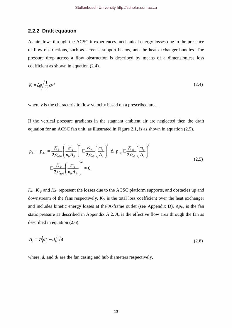
2.2.2 Draft equation

As air flows through the ACSC it experiences mechanical energy losses due to the presence

of flow obstructions, such as screens, support beams, and the heat exchanger bundles. The

pressure drop across a flow obstruction is described by means of a dimensionless loss

coefficient as shown in equation (2.4).

2

2

1vpK ρ∆= (2.4)

where v is the characteristic flow velocity based on a prescribed area.

If the vertical pressure gradients in the stagnant ambient air are neglected then the draft

equation for an ACSC fan unit, as illustrated in Figure 2.1, is as shown in equation (2.5).

02

222

2

56

2

3

2

3

2

5671

≈

+

+∆−

+

=−

frb

a

a

t

e

a

a

doFs

e

a

a

up

frb

a

a

tsaa

An

mK

A

mKp

A

mK

An

mKpp

ρ

ρρρ

θ

(2.5)

Kts, Kup and Kdo represent the losses due to the ACSC platform supports, and obstacles up and

downstream of the fans respectively. Kθt is the total loss coefficient over the heat exchanger

and includes kinetic energy losses at the A-frame outlet (see Appendix D). ∆pFs is the fan

static pressure as described in Appendix A.2. Ae is the effective flow area through the fan as

described in equation (2.6).

( ) 422hce ddA −= π (2.6)

where, dc and dh are the fan casing and hub diameters respectively.


14

3. Numerical modelling

3.1 CFD code overview

The commercially available CFD code, FLUENT, was used in this study. This section will

discuss the governing equations, numerical methods and models, and boundary conditions

applied in this study.

3.1.1 Governing equations

The governing equations of fluid flow represent mathematical statements of the conservation

laws of mass, momentum and energy (Versteeg and Malalasekera, 2007). FLUENT

numerically solves these equations using the finite volume method relevant to viscous

incompressible fluids. The governing equations are presented in Table 3.1.

Table 3.1: Governing equations for steady flow of a viscous incompressible fluid

Continuity ( ) 0=vdivvρ

x-momentum ( ) ( ) ( )[ ] Mxt Sugraddivx

pvudiv +++

∂∂−= µµρ v

y-momentum ( ) ( ) ( )[ ] Myt Sugraddivy

pvvdiv +++

∂∂−= µµρ v

z-momentum ( ) ( ) ( )[ ] Mzt Sugraddivz

pvwdiv +++

∂∂−= µµρ v

Energy ( ) ( ) ( )[ ] ESTkgraddivvpdivvTdiv +Φ++−= vvρ

In Table 3.1 above vv is the velocity vector as described in equation (3.1) whiletµ is the

turbulent fluid viscosity and will be discussed later.

kwjviuvvvvv ++= (3.1)

where iv

, jv

and kv

are unit vectors in the x, y and z directions respectively.


15

The momentum source terms SMx, SMy and SMz take into account viscous effects and make

provision for the effects of external momentum sources or sinks such as gravity, buoyancy

and flow obstructions. Φ is an energy dissipation term and is defined in equation (3.2).

( )

∂∂+

∂∂+

∂∂+

∂∂+

∂∂+

∂∂+

∂∂+

∂∂+

∂∂

+=Φ2

22222

2

y

w

z

v

x

w

z

u

x

v

y

u

z

w

y

v

x

u

tµµ (3.2)

Finally, the energy source term, SE, makes provision for energy source or sink terms that may

come about as a result of, amongst other phenomena, heat transfer to or from the fluid.

The governing equations are discretized, as described in Section 3.1.2 hereafter, and solved

numerically using the SIMPLE solution algorithm for pressure-velocity coupling (Patankar,

1980).

3.1.2 Discretization

The governing equations are integrated over each control volume or cell in the numerical grid

and then discretized. For convenience consider the generalized form of the steady state

governing equations presented in equation (3.3).

( ) ( )[ ] ϕϕ ϕρϕ Sgraddivvdiv +Γ=r (3.3)

In this equation, by setting the variable φ equal to 1, u, v, w or T and selecting appropriate

values of the diffusion coefficient Γφ and source terms, the equations listed in Table 3.1 are

obtained (Versteeg and Malalasekera, 2007).

Integrating equation (3.3) over a control volume yields,

( ) [ ] dVSdVgraddivdVvdivCVCVCV ∫∫∫ +Γ= ϕϕ ϕρϕ )(

r (3.4)

where V represents the cell volume.


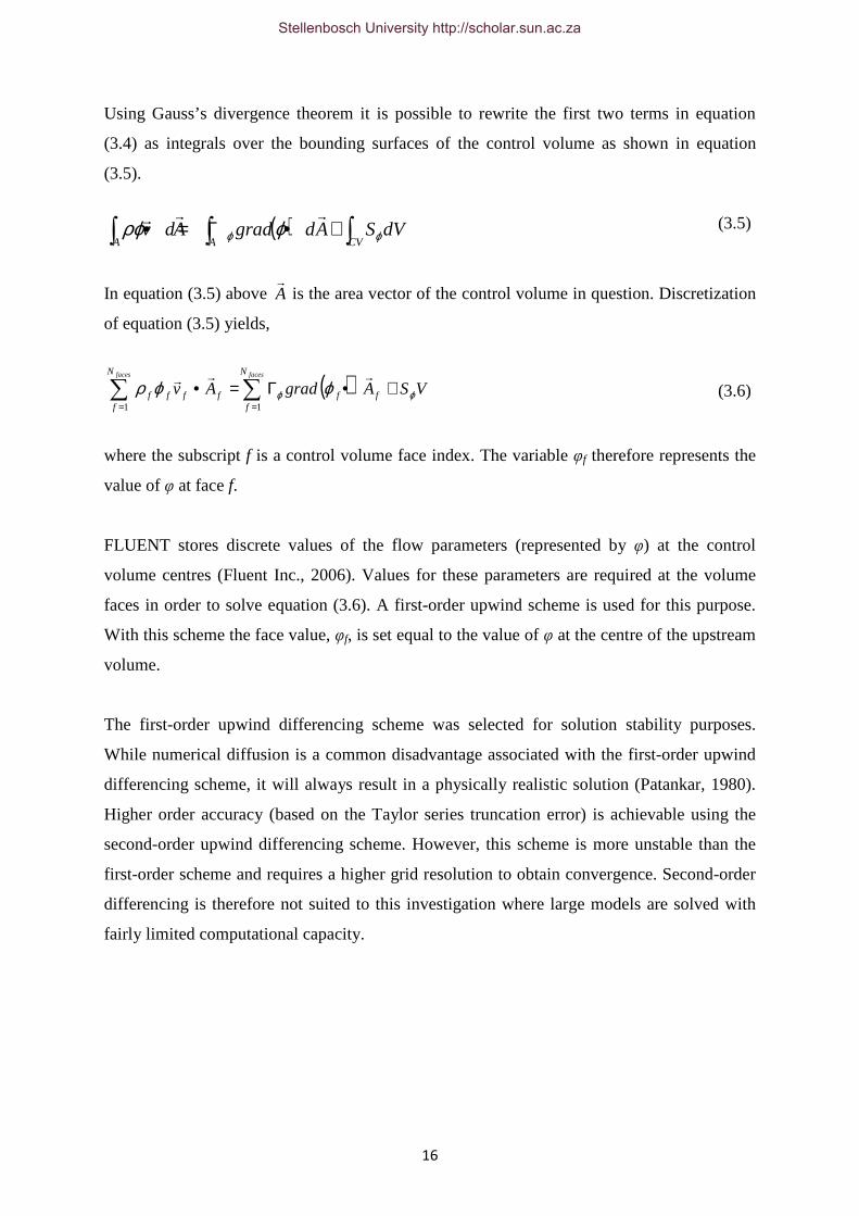
16

Using Gauss’s divergence theorem it is possible to rewrite the first two terms in equation

(3.4) as integrals over the bounding surfaces of the control volume as shown in equation

(3.5).

( ) ∫∫∫ +•Γ=•CVAA

dVSAdgradAdv ϕϕ ϕρϕrrr

(3.5)

In equation (3.5) above A

r is the area vector of the control volume in question. Discretization

of equation (3.5) yields,

( )∑∑==

+•Γ=•facesfaces N

fff

N

fffff VSAgradAv

11ϕϕ ϕϕρ

rrr (3.6)

where the subscript f is a control volume face index. The variable φf therefore represents the

value of φ at face f.

FLUENT stores discrete values of the flow parameters (represented by φ) at the control

volume centres (Fluent Inc., 2006). Values for these parameters are required at the volume

faces in order to solve equation (3.6). A first-order upwind scheme is used for this purpose.

With this scheme the face value, φf, is set equal to the value of φ at the centre of the upstream

volume.

The first-order upwind differencing scheme was selected for solution stability purposes.

While numerical diffusion is a common disadvantage associated with the first-order upwind

differencing scheme, it will always result in a physically realistic solution (Patankar, 1980).

Higher order accuracy (based on the Taylor series truncation error) is achievable using the

second-order upwind differencing scheme. However, this scheme is more unstable than the

first-order scheme and requires a higher grid resolution to obtain convergence. Second-order

differencing is therefore not suited to this investigation where large models are solved with

fairly limited computational capacity.


17

3.1.3 Turbulence model

Turbulence is accounted for using the realizable k-ε turbulence model (Shih et al., 1995). This

model is an improvement on the standard k-ε model (Launder and Spalding, 1974), used by

Bredell (2005) and Van Rooyen (2008), and provides superior performance for flows

involving separation, recirculation, rotation and boundary layers under strong adverse

pressure gradients (Fluent Inc., 2006). The steady state governing equations for the turbulent

kinetic energy, k, and the turbulent energy dissipation rate, ε, in a viscous incompressible

fluid are presented in equations (3.7) and (3.8) respectively.

( ) ( ) kbkk

t SGGkgraddivvkdiv +−++

+= ρε

σµµρ v

(3.7)

( ) ( ) εεε

ενε

ερερεσµµρε SG

kC

kCSCgraddivvdiv b

t +++

−+

+= 1

2

21

v (3.8)

In equations (3.7) and (3.8), Gk and Gb represent the generation of turbulent kinetic energy

due to mean velocity gradients and buoyancy respectively (Fluent Inc., 2006), while Sk and Sε

respectively make provision for additional sources of turbulent kinetic energy or dissipation

rate. The turbulent Prandtl numbers for turbulent kinetic energy and turbulent energy

dissipation rate are represented by σk and σε respectively (see Table 3.2). Furthermore,

( )[ ]54301 += ηη,.maxC (3.9)

where,

εη kS⋅= (3.10)

and S is the modulus of the mean strain rate tensor as described in Shih et al. (1995).

The turbulent viscosity, which appears in Table 3.1 and equations (3.7) and (3.8), is defined

as shown in equation (3.11).

ερµ µ2kCt = (3.11)


18

One of the primary differences between the standard and realizable k-ε turbulence models is

that in the standard model Cµ is a constant while in the realizable model it is a function of the

mean strain and rotation rates, as well as k and ε (Fluent Inc., 2006), as shown in equation

(3.12) below.

1*

0

−

+=

εµkU

BBC s (3.12)

In equation (3.12), Bs is a function of the shear tensor and U* is a function of both the shear

tensor and the rate of rotation of the fluid as described in detail in Shih et al. (1995).

The values of the realizable k-ε turbulence model constants are given in Table 3.2 below.

Table 3.2: Realizable k-ε turbulence model constants

C1ε C2 σk σε B0

1.44 1.90 1.00 1.20 4.04

3.1.4 Buoyancy effects

The effects of buoyancy due to air density gradients, caused by temperature variations in the

flow domain, are taken into account using the Boussinesq model. This model treats density as

a constant value in all the governing equations, except for the buoyancy term in the

momentum equations (see Table 3.1) where the Boussinesq approximation shown in equation

(3.13) is used.

( )T∆−≈ βρρ 10 (3.13)

In equation (3.13) ρ0 is the air density at the ambient temperature, and ∆T represents the

difference between the localized and ambient air temperatures. The thermal expansion

coefficient, β, is approximated as a function of the ambient air temperature as illustrated in

equation (3.14).


19

aT1=β (3.14)

FLUENT also makes provision for the definition of fluid density as a function of

temperature. Use of the Boussinesq model, however, results in more rapid convergence of the

numerical solution than is possible for the previously mentioned case. Furthermore, density

fluctuations as a result of temperature differences are small on average and have a negligible

effect on the governing equations except in the buoyancy terms. Therefore, while the

Boussinesq model results in an additional approximation in the numerical solution, the

convergence rate advantage outweighs this drawback.

3.1.5 Boundary and continuum conditions

The solution of the governing equations requires specified boundary conditions. The

appropriate selection and positioning of these numerical boundaries is of paramount

importance to the accuracy of the results. The boundary conditions used in this study are

discussed hereafter.

a) Velocity boundary: The velocity boundary condition allows the user to specify the inlet

velocity vector on a flow domain boundary. Specification of the temperature and turbulence

parameters is also required. The static pressure varies as required to meet the specified flow

velocity. While this boundary condition is typically used as a flow domain inlet boundary, it

is also possible to use it as an outlet boundary as long as overall continuity is maintained in

the flow domain (Fluent Inc., 2006).

b) Pressure boundary: This boundary condition allows the user to specify the static pressure

at a flow domain boundary where the flow rate and velocity profile across the boundary are

unknown. Pressure boundaries allow flow to enter or leave the flow domain depending on the

conditions adjacent to the boundary. When outflow takes place, the temperature and

turbulence parameters at the boundary are extrapolated from the upstream cells. Inflow from

a pressure boundary is always normal to the boundary and is subject to user specified

temperature and turbulence parameters.


20

c) Wall boundary: This boundary condition is used to model all solid surfaces in the flow

domain. As a default the no-slip condition is applied in FLUENT at the wall surface.

FLUENT does, however, allow the user to specify a surface shear stress. A slip wall

boundary condition can be achieved by setting the wall shear stress equal to zero.

d) Pressure jump fan: FLUENT’s pressure jump fan model applies a discontinuous static-

to-static pressure rise across an infinitely thin face. The pressure rise is determined as a

function of the normal component of the flow velocity immediately upstream of the fan face.

The pressure jump fan method will be described in greater detail in Section 3.2.2.1.

e) Radiator: The radiator boundary condition allows for the specification of a loss

coefficient, of the form described in equation (2.4), and/or heat transfer coefficient based on

the normal component of the flow through an infinitely thin radiator element.

f) Interior face: An interior face has no effect on the flow but provides a defined surface on

which flow parameters can be monitored and/or recorded for later use.

g) Porous zone: A porous zone is a bounded cell zone within the flow domain in which an

empirically determined momentum sink term is added to the governing momentum equations

(Fluent Inc., 2006). The momentum sink term is defined by means of viscous and inertial loss

coefficients (described in Section 3.2.2.2). Provision is also made for the addition of source

or sink terms in the energy equation of the flow as it passes through the zone.

3.2 Numerical ACSC model

Due to computational limitations the numerical modelling of the ACSC was carried out in

two stages. The first stage involves the solution of the flow field in the vicinity of a simplified

representation of the ACSC. This stage is referred to as the global flow field stage. In the

second stage, the ACSC is modelled in detail in a smaller flow domain with boundary

conditions derived from the global flow field simulation results. The global flow field and

detailed models are described in detail in the sections that follow.


21

An iterative solution procedure was followed during the numerical ACSC performance

evaluation. First the global flow field was solved assuming all the fans are operating at the

design point and the air temperature at the heat exchanger outlet is equal to the steam

temperature. The necessary profiles were then extracted from the global flow field and

applied to the boundaries of the detailed model. The predicted fan performances and average

heat exchanger outlet temperature generated during the detailed model simulation were then

used to update the ACSC behaviour in the global flow field model. The global flow field was

subsequently solved again and updated profiles extracted for use in the final detailed model

simulation. The sensitivity of the solution to the number of iterations was investigated and it

was found that a single iteration was sufficient (see Section 4.1.2).

Numerical investigations of ACSCs of similar size to those considered in this study can be

carried out using a single numerical model. The use of a single model simplifies and

accelerates the solution process. However, for much larger installations consisting of many

more fans a single model is not feasible. This investigation therefore serves as a useful means

of evaluating the two-step solution procedure.

3.2.1 Global flow field

A schematic of the global flow field model is presented in Figure 3.1.

Figure 3.1: Schematic of an ACSC, (a) Side elevation, (b) Side elevation

(simplified for global flow field model)

In this model the ACSC is represented by a rectangle with uniform flow velocities specified

across its inlet and outlet. The magnitudes of these velocities depend on the expected

performance of the ACSC fans and the average density of the air at the ACSC inlet and outlet

x

z

x

z

(a) (b)


22

respectively. The default turbulent kinetic energy and turbulent energy dissipation rate values

of k = 1 m2/s2 and ε = 1 m2/s3 provided by FLUENT were applied at these boundaries.

The global flow field model is illustrated in Figure 3.2.

Figure 3.2: Global flow field model

The flow domain sides are modelled using slip walls for straight-flow simulations and

velocity inlet/pressure boundary conditions for cross-flow simulations. In this case straight-

flow refers to a positive x-direction wind, while cross-flow describes a xy-direction wind

(45° with respect to the x-direction). The flow domain roof is modelled using a slip wall for

solution stability purposes. The side and roof boundaries are located sufficiently far from the

ACSC and have a negligible influence on the flow in the region of interest. The ground is

represented by a no slip wall. The dimensions of the El Dorado and generic global flow field

models are included in Table 3.3.

Table 3.3: ACSC dimensions

H i, m Hw, m Lxt, m Lyt, m

El Dorado 19.20 8.27 82.83 74.94

Generic system 20.00 10.00 59.00 63.36

Hw

1000 m

2000 m

2000 m

2000 m B

B

A A

20 m

Hi

Lxt

Lyt

Global inlet

Profile faces

Slip wall Global outlet

Model sides

ACSC model

Side elevation End elevation

Plan

z

x

y

x

y

z


23

A power law wind profile of the form shown in equation (3.15) is specified for the velocity

inlet boundary used to represent the global inlet.

( )biwz Hzvv = (3.15)

In equation (3.15) above, vw is the wind velocity at fan platform height Hi, while b is a

constant. Where experimental data is absent, b = 1/7 as used by Bredell (2005) and Van

Rooyen (2008).

The global outlet boundary is modelled using the pressure boundary condition with a

specified backpressure of 0 N/m2 (gauge). Once again, the default turbulence parameters were

applied at these boundaries.

Interior faces were placed at a distance of 20 m from the ACSC in all directions. Profiles of

x-, y- and z-velocity, temperature, turbulent kinetic energy and turbulent energy dissipation

rate were extracted from the global flow field model on these faces.

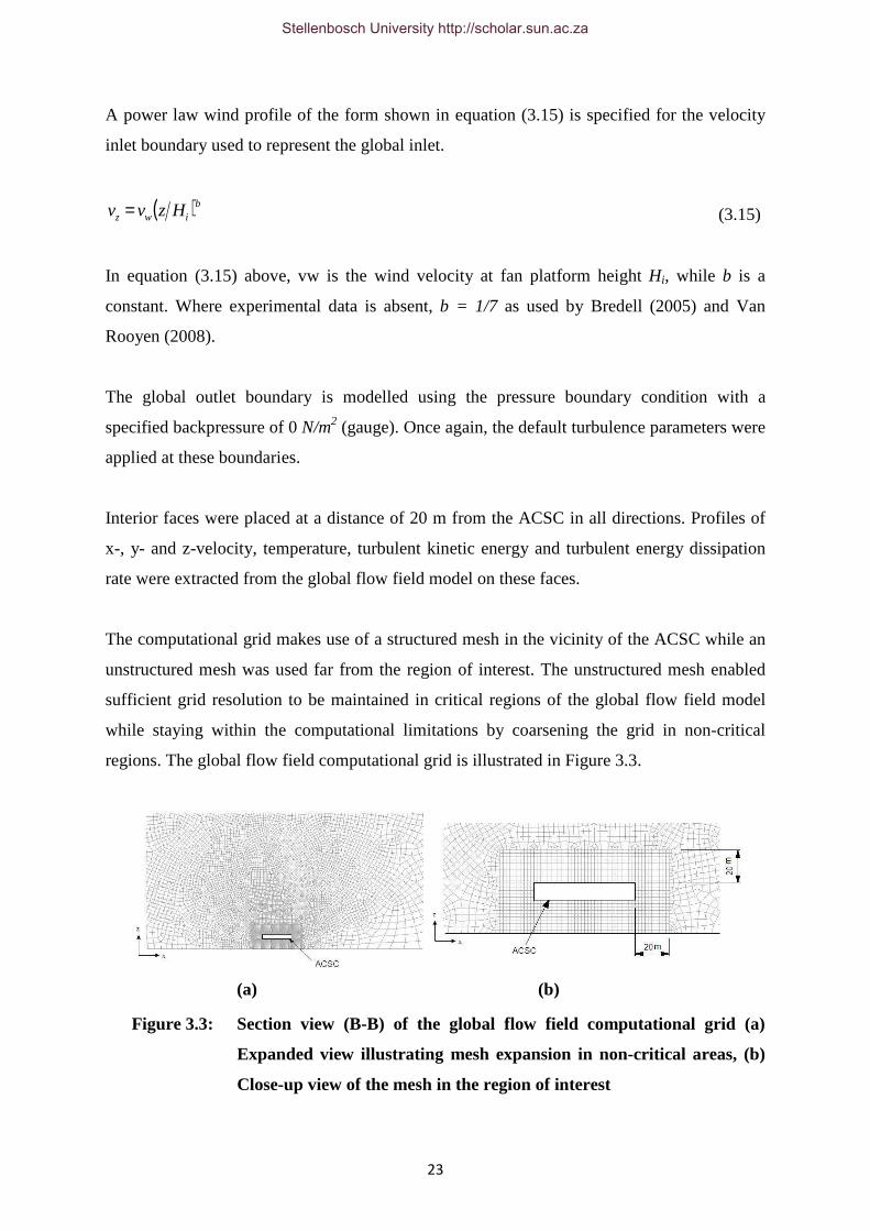
The computational grid makes use of a structured mesh in the vicinity of the ACSC while an

unstructured mesh was used far from the region of interest. The unstructured mesh enabled

sufficient grid resolution to be maintained in critical regions of the global flow field model

while staying within the computational limitations by coarsening the grid in non-critical

regions. The global flow field computational grid is illustrated in Figure 3.3.

(a) (b)

Figure 3.3: Section view (B-B) of the global flow field computational grid (a)

Expanded view illustrating mesh expansion in non-critical areas, (b)

Close-up view of the mesh in the region of interest


24

3.2.2 Detailed ACSC model

A schematic of the detailed ACSC model is shown in Figure 3.4 below (dimensions are as

given in Table 3.3). In this model the ground is represented using the no slip wall boundary

condition. The flow domain boundaries are represented using the velocity boundary condition

and profiles of x-, y- and z-velocity, temperature, turbulent kinetic energy and turbulent

energy dissipation rate, extracted from the global flow field model, are applied to these

boundaries. The ACSC consists of multiple fan units arranged in an array, as described in

Section 1.3. The modelling of each fan unit and its components is described hereafter.

Figure 3.4: Detailed ACSC model schematic

Fan unit

Side elevation

Walkway location

ACSC Flow domain boundaries

Hw

20 m

x

z Hi

Pla

Lxt 20 m 20 m

Lyt

20 m

20 m

Flow domain boundaries Walkway location

x

y

Plan


25

Each ACSC fan unit (see Figure 2.1) consists of a fan inlet shroud, a fan, a plenum chamber

and a heat exchanger; and is modelled as illustrated in Figure 3.5 below.

Figure 3.5: ACSC fan unit, (a) Numerical model, (b) Numerical model dimensions

Table 3.4 gives the dimensions of the fan unit models for El Dorado and the generic ACSC.

The fan and heat exchanger models are described in Sections 3.2.2.1 and 3.2.2.2 respectively.

The computational grid in the vicinity of each fan unit is illustrated in Figure 3.6.

Table 3.4: ACSC fan unit numerical model dimensions

Lx, m Ly, m Lz, m

El Dorado 13.805 14.988 0.2

Generic system 11.8 10.56 0.2

Figure 3.6: Computational grid in the region of each ACSC fan unit

The effect of modelling the actual A-frame heat exchanger as opposed to using the simplified

version (see Figure 3.7) was investigated and was found to have a negligible effect on the

z

x

Heat exchanger model

Plenum chamber

Fan model

Ly

Lx

Hw

z

x

y

Lz

(a) (b)


26

numerically predicted ACSC fan performances. Furthermore, the modelling of the A-frame

did not significantly affect the nature of the flow in the vicinity of the ACSC. A comparison

of the results generated using the different heat exchanger models is included in Appendix

B.1. The use of the simplified ACSC fan unit model is therefore reasonable since the purpose

of this study is to investigate fan and ACSC performance and not the flow in the plenum or at

the heat exchanger outlet (Van Rooyen, 2008).

Figure 3.7: ACSC fan unit models, (a) Simplified version, (b) A-frame version

3.2.2.1 Numerical fan model

The pressure jump method (default FLUENT model) was used to represent the fans in the

detailed ACSC model. As mentioned previously, the pressure jump across the fan is defined

as a static-to-static pressure jump. The pressure jump method calculates the static pressure

jump to be added to the static pressure term in the linear momentum equation in the flow

field immediately upstream of the fan (Van der Spuy et al., 2009) based on a user-defined fan

performance characteristic. This characteristic is sourced from the fan specifications. It must,

however, be noted that the fan static pressure rise, as referred to by suppliers, is actually a

total-to-static pressure rise since performance tests are carried out with a settling chamber

immediately upstream of the fan. It is therefore necessary to add the dynamic pressure at the

fan inlet to the specified fan static pressure characteristic, as described in Appendix C, in

order to ensure realistic performance of the pressure jump fan model.

Due to the lack of information regarding the fan behaviour at very low flow rates or during

backflow, it was assumed that the static-to-static pressure rise across the fan remains constant

under these conditions. This assumption is reasonable since only small segments of a few

fans operate under backflow conditions in the simulations carried out in this study. The

(a) (b)

Heat exchanger

y z

y z

Heat exchanger


27

performance characteristics of the fans used in ACSCs considered in this study are illustrated

in Figure 3.8 below (the units have been removed from El Dorado’s fan performance

characteristic for confidentiality purposes).

(a)

(b)

Figure 3.8: Fan performance characteristics (a) El Dorado, (b) Generic system

3.2.2.2 Heat exchanger model

The heat exchanger is modelled using FLUENT’s porous zone continuum condition which

accounts for losses in the mechanical energy of the air due to the effective system resistance

to the flow, as well as heat transfer to the air.

-500 0 500 1000

∆p

F, N

/m2

VF, m3/s

Specified fan performance data

Fan static pressure characteristic

Adjusted characteristic including

assumptions

0

50

100

150

200

250

300

350

400

450

-500 0 500 1000 1500

Δp

F, N

/m2

VF, m3/s

Specified fan

performance data

Fan static pressure

characteristic

Adjusted characteristic

including assumptions

dF = 10.362 m

Ψ = 5.3°

ρa = 1.128 kg/m3

N = 99 rpm

dF = 9.145 m

Ψ = 34.5°

ρa = 1.0857 kg/m3

N = 125 rpm


28

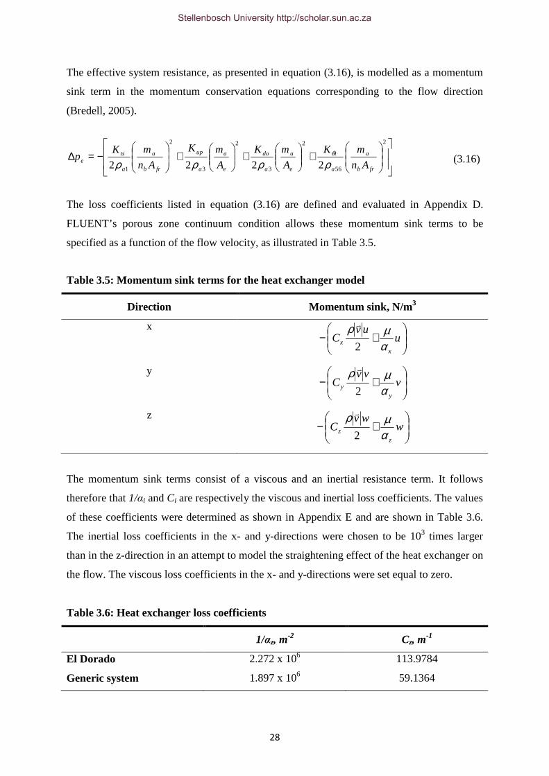
The effective system resistance, as presented in equation (3.16), is modelled as a momentum

sink term in the momentum conservation equations corresponding to the flow direction

(Bredell, 2005).

+

+

+

−=∆

2

56

2

3

2

3

2

1 2222 frb

a

a

t

e

a

a

do

e

a

a

up

frb

a

a

tse An

mK

A

mK

A

mK

An

mKp

ρρρρθ (3.16)

The loss coefficients listed in equation (3.16) are defined and evaluated in Appendix D.

FLUENT’s porous zone continuum condition allows these momentum sink terms to be

specified as a function of the flow velocity, as illustrated in Table 3.5.

Table 3.5: Momentum sink terms for the heat exchanger model

Direction Momentum sink, N/m3

x

+− u

uvC

xx α

µρ2

v

y

+− v

vvC

yy α

µρ2

v

z

+− w

wvC

zz α

µρ2

v

The momentum sink terms consist of a viscous and an inertial resistance term. It follows

therefore that 1/αi and Ci are respectively the viscous and inertial loss coefficients. The values

of these coefficients were determined as shown in Appendix E and are shown in Table 3.6.

The inertial loss coefficients in the x- and y-directions were chosen to be 103 times larger

than in the z-direction in an attempt to model the straightening effect of the heat exchanger on

the flow. The viscous loss coefficients in the x- and y-directions were set equal to zero.

Table 3.6: Heat exchanger loss coefficients

1/αz, m-2 Cz, m

-1

El Dorado 2.272 x 106 113.9784

Generic system 1.897 x 106 59.1364


29

An energy source term of the form shown in equation 3.17 is added to the energy

conservation equation to account for heat transfer to the air as it passes through the heat

exchanger. The derivation of this source term and its application in the numerical model are

illustrated in Appendix F.

( ) zaiaopaaE LTTcwS −= ρ (3.17)

3.2.3 Ideal flow model

In order to determine the effects of wind on fan performance in an ACSC it is first necessary

to determine the performance of the fan when operating under ideal flow conditions. A

schematic of the numerical model used for this purpose is shown in Figure 3.9. The fan unit

model is as described in Section 3.2.2.

Figure 3.9: Ideal flow model schematic

The numerical grid employed in the ideal flow model is illustrated in Figure 3.10 below. The

meshing of the fan unit is as illustrated in Figure 3.6.

Figure 3.10: Ideal flow model computational mesh

Fan unit

x

z

8dF 5dF

φ4dF

Pressure boundaries

Air flow Outlet Inlet


30

This model allowed the numerically determined operating point under ideal flow conditions

to be compared to the theoretically calculated operating point to ensure that no significant

errors had been introduced into the system through some of the assumptions and numerical

simplifications made. A comparison of the two is illustrated in Appendix B.2.

3.3 Performance measures

In order to evaluate the performance of an ACSC and its components it is necessary to

identify performance measures that provide meaningful information. In this study three

performance measures were identified and utilized.

a) Fan volumetric effectiveness describes the performance of individual ACSC fans by

comparing the volumetric flow rate through the fan under the prescribed operating conditions

to the volumetric flow rate through the fan under ideal conditions.

Volumetric effectiveness = )(idFF VV (3.18)

Fan volumetric effectiveness is a useful means of identifying where fan inlet distortions are

most severe.

b) Heat transfer effectiveness describes the performance of individual ACSC fan units by

comparing the heat transfer rate achieved by the fan unit under the prescribed operating

conditions to the heat transfer rate expected under ideal operating conditions. The heat

transfer rate associated with a fan unit is given by,

( )aivpaa TTcemQ −= (3.19)

where e is the heat transfer effectiveness of the finned tube heat exchanger as described in

Section 2.2.1. The thermal effectiveness is defined as,

Heat transfer effectiveness = idQQ (3.20)


31

This measure can also be applied to an ACSC consisting of nF fan units to determine the

overall thermal effectiveness.

Overall heat transfer effectiveness = idF

n

jj QnQ

F

∑=1

(3.21)

Heat transfer effectiveness takes into account the combined effects of reduced fan

performance due to inlet distortions and plume recirculation, and is therefore a useful

indicator of the effects of wind on ACSC performance.

c) Steam turbine backpressure is used as the final performance measure in this study. It has

been mentioned previously that a dynamic relationship exists between the ACSC and the

steam turbine, and that reduced ACSC performance results in increased turbine backpressure.

Turbine backpressure is also monitored continuously at the power plant. It follows that steam

turbine backpressure is a useful indicator of overall ACSC performance.

In order to calculate the steam turbine backpressure it is assumed that the heat rejected by the

ACSC is constant for a given operating point regardless of wind conditions. This is untrue

since the steam turbine efficiency is related to backpressure. The turbine efficiency therefore

fluctuates with ACSC performance. For the same heat input, the heat to be rejected by the

ACSC must therefore fluctuate along with the turbine backpressure. As a first approximation,

however, it is useful to make the assumption that the heat rejected by the ACSC is constant.

The heat rejected by the ACSC under prescribed operating conditions is calculated as the sum

of the heat rejected by each of the ACSC fan units.

( )∑=

−=Fn

jaijactualvjpaaj TTecmQ

1)( (3.22)

The heat transfer rate for the entire ACSC under ideal conditions can be calculated as shown

in equation (3.23)

)( )()( aidvidpaidaFid TTecmnQ −= (3.23)


32

Rearranging equation (3.22) and equating it to equation (3.23) yields the following

expression used to calculate the actual steam turbine exhaust temperature under prescribed

operating conditions,

∑∑

∑∑

= =

= =

+=

6

1

5

1

6

1

5

1)(

i jijpaaij

i jaijijpaaijid

actualv

ecm

TecmQ

T (3.24)

This actual steam turbine exhaust temperature can then be used to determine the steam

turbine backpressure using equations (3.25) and (3.26), as given by Kröger (2004).

zvp 10= , N/m2 (3.25)

where,

( ) ( )( )[ ]

( )[ ] 786118312.2110102873.4

1011050474.1

16.273log02808.516.273179586.10

)(

)(

16.273176955.44

116.27329692.84

)(10)(

+−×+

−×+

+−=

−−

−−−

actualv

actualv

T

T

actualvactualv TTz

(3.26)


33

4. Evaluation of the numerical models

The accuracy of the numerical models used in this study will be examined in this section

through a sensitivity analysis, as well as through a comparison of the results to test data and

previous numerical work. The fan numbering scheme used hereafter is illustrated in Figure

4.1.

Figure 4.1: Fan numbering scheme, (a) El Dorado, (b) Generic ACSC

4.1 Sensitivity analysis

Various user controllable model parameters have an influence on the accuracy of the results

generated during a numerical simulation. It is necessary to design the numerical model to be

as insensitive to these parameters as possible. The effects of grid resolution, profile boundary

proximity to the ACSC, and global-to-detailed model iteration frequency are investigated in

this section. The analyses were carried out using the generic ACSC subject to a straight-flow

wind speed of vw = 3 m/s.

4.1.1 Grid resolution

The effect of grid resolution on the numerical results was investigated through both manual

and adaptive mesh refinement techniques. Special attention was paid to the region of the fan

inlets and the upstream edge of the fan platform since it is expected that this is where

(1,6) (2,6) (3,6) (4,6) (5,6)

(1,5) (2,5) (3,5) (4,5) (5,5)

(1,4) (2,4) (3,4) (4,4) (5,4)

(1,3) (2,3) (3,3) (4,3) (5,3)

(1,2) (2,2) (3,2) (4,2) (5,2)

(1,1) (2,1) (3,1) (4,1) (5,1)

(1,1) (2,1) (3,1) (4,1) (5,1) (6,1)

(1,4) (2,4) (3,4) (4,4) (5,4) (6,4)

(1,5) (2,5) (3,5) (4,5) (5,5) (6,5)

(1,3) (2,3) (3,3) (4,3) (5,3) (6,3)

(1,2) (2,2) (3,2) (4,2) (5,2) (6,2)

Wind screen

(a) (b)


34

separation is likely to be most severe and, therefore, sufficient grid resolution most important.

The effect of grid resolution on the numerical results is illustrated in Figure 4.2 for the cases

described in Table 4.1.

Table 4.1: Grid resolution sensitivity cases: manual adaptation

Grid case number Total number of cells Number of cells on fan face

1 701 620 90

2 2 669 488 348

3 3 572 915 864

Figure 4.2: The effect of grid resolution on the predicted volumetric effectiveness

of certain ACSC fans

Figure 4.2 indicates that the numerical results for grid cases 2 and 3 are similar and as such

grid refinement beyond that of case 2 is not necessary. It can be concluded that the grid used

in case 2 is of sufficient resolution that the results are largely grid independent.

Adaptive meshing was also used to investigate grid dependence in the numerical model.

FLUENT’s dynamic adaptive grid tool allows the user to run simulations where the grid is

automatically refined in regions where a flow parameter gradient exceeds a set value.

Gradients of static pressure were selected as the grid refinement criterion in an attempt to

isolate grid refinement to the primary regions of interest, namely, in the vicinity of the fans

0.0

0.2

0.4

0.6

0.8

1.0

1.2

(1,1) (1,2) (1,3) (3,1) (3,2) (3,3) (5,1) (5,2) (5,3)

VF/

VF

(id

)

Fan no.

Grid 1 Grid 2 Grid 3


35

and in regions where separation occurs. Grid case 1 was used as the starting point and the

solution finally converged at a grid resolution of 1.326x106 total cells with 1440 cells on the

upstream fan faces. The predicted fan volumetric effectivenesses were comparable to those

generated using grid case 2. The higher grid resolution on the fan face in the adaptive

meshing solution, as opposed to grid case 2, can be attributed to the fact that FLUENT refines

the grid in regions of high static pressure gradient. The static pressure discontinuity across the

fan face will result in this face being refined during every refining operation.

Grid case 2 is of sufficient resolution that further mesh refinement is not justified. This grid

was used in all simulations carried out as part of this study.

4.1.2 Boundary proximity

The effect of the proximity of the profile faces to the ACSC was investigated. These faces are

the surfaces on which the necessary profiles are extracted from the global flow field model

(see Figure 3.2), and form the flow domain boundaries in the detailed model (see Figure 3.4).

The cases described below, and illustrated in Figure 4.3, were considered.

a) Case 1: All boundaries located 20 m from the ACSC (as for Figure 3.2).

b) Case 2: The upstream and downstream boundaries were moved to 50 m (x-direction

expansion) while the top and side boundaries remained at 20 m.

c) Case 3: The side boundaries were moved to 50 m (y-direction expansion) while the

upstream, downstream and top boundaries remained at 20 m.

d) Case 4: The top boundary was moved to 50 m (z-direction expansion) while the

upstream, downstream and side boundaries remained at 20 m.


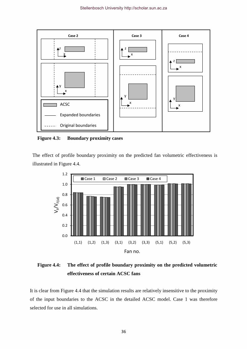
36

Figure 4.3: Boundary proximity cases

The effect of profile boundary proximity on the predicted fan volumetric effectiveness is

illustrated in Figure 4.4.

Figure 4.4: The effect of profile boundary proximity on the predicted volumetric

effectiveness of certain ACSC fans

It is clear from Figure 4.4 that the simulation results are relatively insensitive to the proximity

of the input boundaries to the ACSC in the detailed ACSC model. Case 1 was therefore

selected for use in all simulations.

0.0

0.2

0.4

0.6

0.8

1.0

1.2

(1,1) (1,2) (1,3) (3,1) (3,2) (3,3) (5,1) (5,2) (5,3)

VF/

VF

(id

)

Fan no.

Case 1 Case 2 Case 3 Case 4

ACSC

Expanded boundaries

Original boundaries

Case 2

y

x

z

x

Case 4

x

y

x

z

Case 3

x

y

x

z


37

4.1.3 Global-to-detailed ACSC model iteration frequency

The iterative process followed during the numerical simulation of ACSC performance was

described in Section 3.2. The effect of the number of global-to-detailed ACSC model

iterations was investigated using the cases described below. A comparison of the simulation

results, presented in Figure 4.5, clearly indicates that only a single iteration is necessary.

a) Zero iterations: The profiles used in the detailed model are extracted from the global

flow field model with the ACSC inlet and outlet velocities based on fan performance under

ideal conditions.

b) Single iteration: The ACSC inlet and outlet velocities in the global flow field model are

updated using the predicted fan performance based on the zero iteration boundary profiles.

The updated profiles from the global flow field are then used in the detailed model.

c) Double iteration: The fan performance determined in the detailed ACSC model based

on the single iteration boundary profiles is used to determine the ACSC inlet and outlet

velocities in the global flow field model and generate an updated set of profiles for use in the

detailed model.

Figure 4.5: The effect of global-to-detailed ACSC model iteration frequency on

the predicted volumetric effectiveness of certain ACSC fans

0.0

0.2

0.4

0.6

0.8

1.0

1.2

(1,1) (1,2) (1,3) (3,1) (3,2) (3,3) (5,1) (5,2) (5,3)

VF/

VF

(id

)

Fan no.

Zero iterations Single iteration Double iteration


38


test data

In any numerical investigation it is necessary to validate the results through a comparison

with test or experimental data. Full scale ACSC performance tests were carried out at El

Dorado during September 2007 as described in Owen (2007). The data collected during these

tests will be used for the purpose of verification of the numerical models employed in this

study.

4.2.1 Turbine operation under ideal conditions

In order to determine the effect of various parameters on ACSC performance it is first

necessary to know how the ACSC is expected to perform under ideal operating conditions.

The turbine performance under ideal conditions is illustrated in Figure 4.6 (units have been

removed for the purpose of confidentiality). This characteristic is based on test data for

periods where there was no wind present (vw ≤ 0.5 m/s) and all ACSC fans were operating at

full speed.

Figure 4.6: Turbine performance under ideal conditions

A curve fit through the data yields a power law relationship between turbine backpressure

and ambient temperature (in °C) under ideal operating conditions with all ACSC fans

operating at full speed, as illustrated in equation (4.1).

21)(

Caidv TCp = (4.1)

0

5000

10000

15000

20000

25000

20 25 30 35 40 45

pv,

N/m

2

Ta, °C


39

The turbine exhaust steam temperature, calculated as being the saturation temperature of

steam at the turbine backpressure, is determined according to equation (4.2), as given by

Kröger (2004).

)ln(10437169.1)ln(161488.161001204.7

10738954.31027215.410832295.1630366.164425

132103

vvvv

vvvv

pppp

pppT−−

−−−

×−+×−

×+×+×+=

(4.2)

4.2.2 Test operating points

Periods of relatively stable wind conditions needed to be identified to provide suitable data

for comparison with the numerical results. Wind speed stability was the primary

consideration in the selection of suitable test periods. It was, however, attempted to select

periods exhibiting consistent wind directions as well. Ultimately, four test periods, described

in Table 4.2, were identified for comparison with the numerical results. Full descriptions of

the wind and temperature data for each test period are included in Appendix G.

Table 4.2: Test data operating points

TP1 TP2 TP3 TP4

Ta, °C 30.1814 38.4999 36.2650 32.7049

pv(actual), N/m2 14078.29 20692.84 18615.79 14164.87

vw, m/s 5.5981 11.4495 7.9316 4.3333

θw, ° 206.2440 234.1740 236.503 261.1180

b 0.2850 0.2040 0.2179 0.1475

mv, kg/s 128.9389 132.6066 131.1391 128.4598

In Table 4.2 Ta is the ambient temperature at fan platform height, pv(actual) is the pressure

measured at the turbine exhaust. The mean wind direction over the test period is given by θw.

The wind velocity at fan platform height and power law exponent, as described in equation

(3.15), are given by vw and b respectively. The mass flow rate of dry steam measured at the

turbine exhaust is represented by mv.


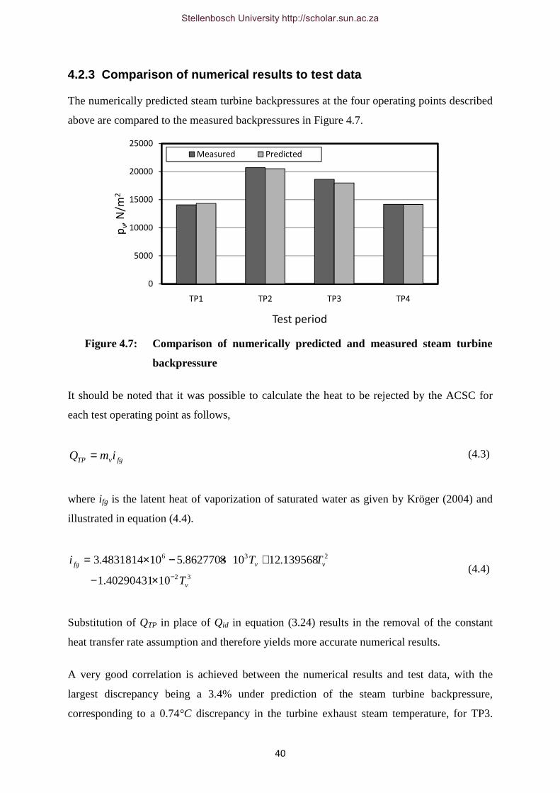
40

4.2.3 Comparison of numerical results to test data

The numerically predicted steam turbine backpressures at the four operating points described

above are compared to the measured backpressures in Figure 4.7.

Figure 4.7: Comparison of numerically predicted and measured steam turbine

backpressure

It should be noted that it was possible to calculate the heat to be rejected by the ACSC for

each test operating point as follows,

fgvTP imQ = (4.3)

where i fg is the latent heat of vaporization of saturated water as given by Kröger (2004) and

illustrated in equation (4.4).

32

236

1040290431.1

139568.12108627703.5104831814.3

v

vvfg

T

TTi−×−

+×−×= (4.4)

Substitution of QTP in place of Qid in equation (3.24) results in the removal of the constant

heat transfer rate assumption and therefore yields more accurate numerical results.

A very good correlation is achieved between the numerical results and test data, with the

largest discrepancy being a 3.4% under prediction of the steam turbine backpressure,

corresponding to a 0.74°C discrepancy in the turbine exhaust steam temperature, for TP3.

0

5000

10000

15000

20000

25000

TP1 TP2 TP3 TP4

pv,

N/m

2

Test period

Measured Predicted


41

Possible reasons for the small discrepancies include slight instabilities in the ambient

conditions over the test periods (fluctuations in wind speed and direction for example); as

well as numerical inaccuracies brought about by the pressure jump fan model, two step

modelling approach and simplified heat exchanger model.


previous numerical work

Van Rooyen (2008) carried out a numerical performance analysis on the generic ACSC

considered in this study. The results generated using the numerical model described in this

document will be compared to those presented by Van Rooyen (2008) in this section. Straight

and cross-flow wind speeds of vw = 3 m/s, vw = 6 m/s and vw = 9 m/s were considered. Figure

4.8 illustrates a comparison of the numerically predicted volumetric effectivenesses of

selected ACSC fans.

(a)

(b)

Figure 4.8: Comparison of the numerically predicted volumetric effectivenesses of

fans in (a) the upstream fan row, and (b) non-upstream fan rows,

under straight-flow wind conditions

0.00.10.20.30.40.50.60.70.80.91.01.1

0 3 6 9 12

VF/

VF

(id

)

vw, m/s

Van Rooyen

(2008) (1,1)Present (1,1)

Van Rooyen

(2008) (1,3)Present (1,3)

0.00.10.20.30.40.50.60.70.80.91.01.1

0 3 6 9 12

VF/

VF

(id

)

vw, m/s

Van Rooyen (2008) (3,3)

Present (3,3)

Van Rooyen (2008) (5,3)

Present (5,3)

pa = 90000 N/m2

Ta = 15.6 °C

Tv = 60 °C

pa = 90000 N/m2

Ta = 15.6 °C

Tv = 60 °C


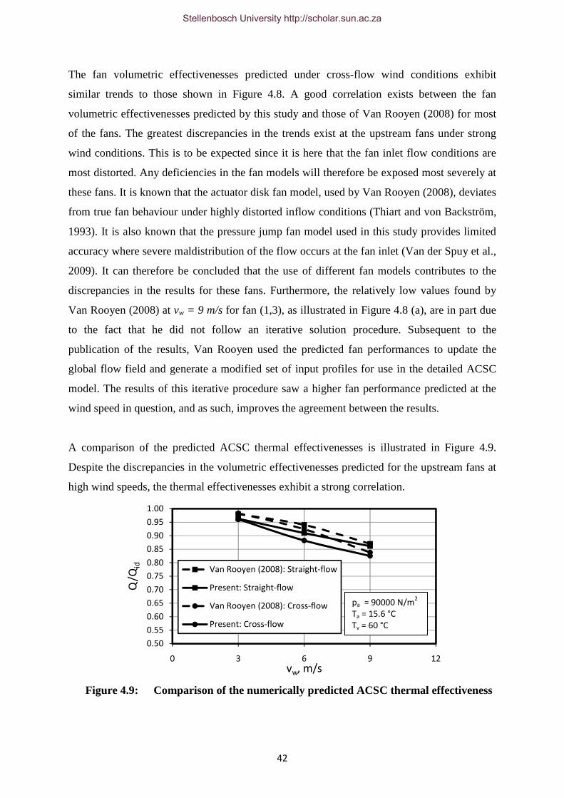
42

The fan volumetric effectivenesses predicted under cross-flow wind conditions exhibit

similar trends to those shown in Figure 4.8. A good correlation exists between the fan

volumetric effectivenesses predicted by this study and those of Van Rooyen (2008) for most

of the fans. The greatest discrepancies in the trends exist at the upstream fans under strong

wind conditions. This is to be expected since it is here that the fan inlet flow conditions are

most distorted. Any deficiencies in the fan models will therefore be exposed most severely at

these fans. It is known that the actuator disk fan model, used by Van Rooyen (2008), deviates

from true fan behaviour under highly distorted inflow conditions (Thiart and von Backström,

1993). It is also known that the pressure jump fan model used in this study provides limited

accuracy where severe maldistribution of the flow occurs at the fan inlet (Van der Spuy et al.,

2009). It can therefore be concluded that the use of different fan models contributes to the

discrepancies in the results for these fans. Furthermore, the relatively low values found by

Van Rooyen (2008) at vw = 9 m/s for fan (1,3), as illustrated in Figure 4.8 (a), are in part due

to the fact that he did not follow an iterative solution procedure. Subsequent to the

publication of the results, Van Rooyen used the predicted fan performances to update the

global flow field and generate a modified set of input profiles for use in the detailed ACSC

model. The results of this iterative procedure saw a higher fan performance predicted at the

wind speed in question, and as such, improves the agreement between the results.

A comparison of the predicted ACSC thermal effectivenesses is illustrated in Figure 4.9.

Despite the discrepancies in the volumetric effectivenesses predicted for the upstream fans at

high wind speeds, the thermal effectivenesses exhibit a strong correlation.

Figure 4.9: Comparison of the numerically predicted ACSC thermal effectiveness

0.50

0.55

0.60

0.65

0.70

0.75

0.80

0.85

0.90

0.95

1.00

0 3 6 9 12

Q/Q

id

vw, m/s

Van Rooyen (2008): Straight-flow

Present: Straight-flow

Van Rooyen (2008): Cross-flow

Present: Cross-flow

pa = 90000 N/m2

Ta = 15.6 °C

Tv = 60 °C


43

5. ACSC performance under windy conditions

Since air is used as the cooling medium in ACSCs, the achievable heat transfer rate is

strongly influenced by atmospheric conditions. Gadhamshetty et al. (2006) mentions

reductions in ACSC cooling effectiveness of up to 10% under unfavourable atmospheric

conditions, namely strong winds and high ambient temperatures. Figure 5.1 illustrates the

numerically predicted effect of wind and ambient temperature on ACSC heat transfer

effectiveness at El Dorado.

(a)

(b)

Figure 5.1: Effect of ambient conditions on ACSC heat transfer effectiveness under

(a) Straight-flow, and (b) cross-flow wind conditions

Figure 5.1 clearly illustrates the negative effect of both high ambient temperatures and strong

winds on ACSC performance. It can be seen that an increase in ambient temperature of ∆Ta =

0.84

0.86

0.88

0.90

0.92

0.94

0.96

0.98

1.00

1.02

10 20 30 40

Q/Q

id

Ta, °C

vw = 3 m/s vw = 6 m/s vw = 9 m/s

0.84

0.86

0.88

0.90

0.92

0.94

0.96

0.98

1.00

1.02

10 20 30 40

Q/Q

id

Ta, °C

vw = 3 m/s vw = 6 m/s vw = 9 m/s


44

20°C results in a decrease in ACSC heat transfer effectiveness in the region of 4%, while

increasing the wind speed from vw =3 m/s to vw = 9 m/s, at a constant ambient temperature

results in a heat transfer effectiveness reduction in the region of 8%. It is clear that wind has a

significant impact on ACSC performance. The effect of winds on ACSC performance will

therefore be the focus of this study.

The effect of the decreased ACSC heat transfer effectiveness, illustrated in Figure 5.1, on the

steam turbine backpressure, is illustrated in Figure 5.2. The trends exhibited in this figure

correspond well with those identified by Maulbetsch and DiFilippo (2007) using test data

from a number of ACSCs.

(a)

(b)

Figure 5.2: Effect of ambient conditions on steam turbine backpressure under (a)

Straight-flow, and (b) cross-flow wind conditions

6000

8000

10000

12000

14000

16000

18000

10 20 30 40

pv,

N/m

2

Ta, °C

vw = 3 m/s

vw = 6 m/s

vw = 9 m/s

No Wind

6000

8000

10000

12000

14000

16000

18000

20000

10 20 30 40

pv,

N/m

2

Ta, °C

vw = 3 m/s

vw = 6 m/s

vw = 9 m/s

No Wind


45

Duvenhage and Kröger (1996) found that the negative effects of wind are as a result of

reduced fan performance, brought about by distorted flow at the fan inlets, and hot plume

recirculation. These phenomena will be examined in more detail hereafter.

5.1 Reduced fan performance due to distorted inlet conditions

Reduced fan performance due to distorted flow at the fan inlets occurs predominantly at the

windward, or leading edge, fans. Previous studies have found reductions in the flow rates

through these fans to be as high as 50% to 70% (Maulbetsch, 2008; McGowan et al., 2008).

Figure 5.3 illustrates the numerically predicted fan volumetric effectivenesses for El Dorado

under straight-flow wind conditions.

Figure 5.3: Fan volumetric effectiveness under straight-flow wind conditions

It can be seen that the performance of the windward fans, namely fans (1,1) - (1,5), are the

worst affected by wind. This is the result of distorted, or off-axis, flow conditions at the inlet

to these fans caused by separation of the flow as it strikes the upstream edge of the ACSC.

Figure 5.4 illustrates the low pressure zone under fan (1,1), as well as the off-axis flow at the

fan inlet, caused by this separation.

0.0

0.2

0.4

0.6

0.8

1.0

1.2

1.4

(1,1

)

(1,3

)

(1,5

)

(2,2

)

(2,4

)

(3,1

)

(3,3

)

(3,5

)

(4,2

)

(4,4

)

(5,1

)

(5,3

)

(5,5

)

(6,2

)

(6,4

)

VF/

VF

(id

)

Fan no.

vw = 3 m/s vw = 6 m/s vw = 9 m/s


(a)

Figure 5.4: Reason for the reduced performance of the windward fans:

(a) Static pressure (

through the centre of fan (1,1) for a straight wind speed of

It should also be noted that the fans located immediately upstream of the windscreens,

namely fans (2,1) - (2,5) and (3,1)

predicted that the performance of some of these fans can be enhanced above that achieved

under ideal conditions. This can be attributed to the stagnation effect of the wind screens on

the flow immediately upstream of their loca

Figure 5.5: Static pressure (

vw = 9m/s

46

Reason for the reduced performance of the windward fans:

(a) Static pressure (ps, N/m2), and (b) Vector plot (v, m/

through the centre of fan (1,1) for a straight wind speed of


(2,5) and (3,1) - (3,5), perform well under windy conditions. It is



the flow immediately upstream of their location, as illustrated in Figure 5.5.

Static pressure (ps, N/m2) along a fan row for a straight wind speed of

(b)

Reason for the reduced performance of the windward fans:

v, m/s) on a section

through the centre of fan (1,1) for a straight wind speed of vw = 9m/s


nder windy conditions. It is



tion, as illustrated in Figure 5.5.

) along a fan row for a straight wind speed of


47

The installation of windscreens therefore holds potential for improving ACSC performance

under windy conditions and warrants further investigation. With El Dorado's current screen

configuration, however, the fans immediately downstream of the windscreens perform

relatively poorly. It is suspected that the current screen configuration may be causing an

excessive blockage effect and is effectively suffocating the downstream fans. The

identification of some optimum windscreen configuration where the performance of the

upstream fans is improved without reducing the performance of the downstream fans

significantly would be a worthwhile exercise and is addressed later in this document.

5.2 Hot plume recirculation

Hot plume recirculation is predominant at the downstream ACSC edges and corners, as

illustrated in Figure 5.6 where the inlet temperatures of the fans (5,1) - (5,5) and (6,1) - (6,5)

are higher than the ambient temperature of Ta = 19.44°C.

Figure 5.6: Inlet temperatures at ACSC fans under straight-flow wind conditions

Plume recirculation is caused by entrainment of hot air from the heat exchanger outlet in

vortex's that form from the leading edge of the fan platform under windy conditions. Figure

5.7 illustrates the vortex formed at El Dorado's ACSC for a straight wind speed of vw = 9 m/s.

The size of the vortex increases in the downstream direction resulting in increased

entrainment of the plume. Eventually the vortex diameter grows large enough to force hot air

below the fan platform and into the region from which the fans draw their air. The

downstream fans lie in this large vortex region and are therefore worst affected by plume

0

5

10

15

20

25

30

(1,1

)

(1,3

)

(1,5

)

(2,2

)

(2,4

)

(3,1

)

(3,3

)

(3,5

)

(4,2

)

(4,4

)

(5,1

)

(5,3

)

(5,5

)

(6,2

)

(6,4

)

Ti,

°C

Fan no.

vw = 3 m/s vw = 6 m/s vw = 9 m/s


48

recirculation. Figure 5.6 also illustrates an increase in the severity of recirculation with

increasing wind speed. This can be attributed to the plume being forced closer to horizontal

with increasing wind speed. This effect is shown in Figure 5.8

Figure 5.7: Vortex formed due to the presence of a straight wind (vw = 9m/s)

Figure 5.8: Plume angle for straight wind speeds of (a) vw = 3 m/s,

(b) vw = 6 m/s, and (c) vw = 9 m/s

5.3 Identification of the primary cause of ACSC performance

reduction under windy conditions

Maulbetsch (2008) states that, at the ACSCs tested by him, the effect of hot plume

recirculation on ACSC performance is small for most wind conditions while fan performance

reductions are often significant. The separate effects of reduced fan performance and plume

recirculation on ACSC heat transfer effectiveness, as well as the effect of the two phenomena

combined, is illustrated in Figure 5.9. Reduced fan performance is clearly the largest


49

contributor to the reduction in ACSC performance under windy conditions and will

subsequently be the focus of the remainder of this study.

Figure 5.9: Illustration of the contribution of reduced fan performance and hot

plume recirculation to reduced ACSC performance under straight-flow

wind conditions at El Dorado

0.80

0.84

0.88

0.92

0.96

1.00

1.04

0 3 6 9 12

Q/Q

id

vw, m/s

Recirculation

Reduced fan performance

Combined effect


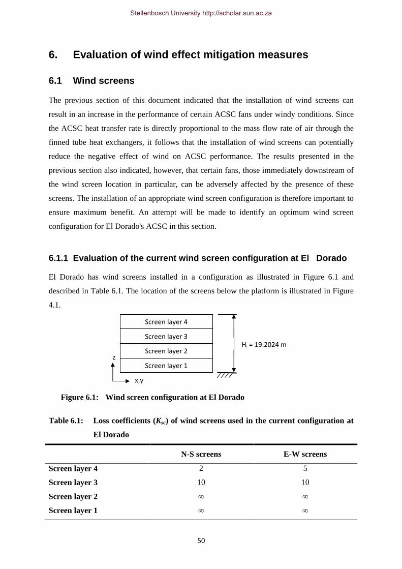
50

6. Evaluation of wind effect mitigation measures

6.1 Wind screens

The previous section of this document indicated that the installation of wind screens can

result in an increase in the performance of certain ACSC fans under windy conditions. Since

the ACSC heat transfer rate is directly proportional to the mass flow rate of air through the

finned tube heat exchangers, it follows that the installation of wind screens can potentially

reduce the negative effect of wind on ACSC performance. The results presented in the

previous section also indicated, however, that certain fans, those immediately downstream of

the wind screen location in particular, can be adversely affected by the presence of these

screens. The installation of an appropriate wind screen configuration is therefore important to

ensure maximum benefit. An attempt will be made to identify an optimum wind screen

configuration for El Dorado's ACSC in this section.

6.1.1 Evaluation of the current wind screen configuration at El Dorado

El Dorado has wind screens installed in a configuration as illustrated in Figure 6.1 and

described in Table 6.1. The location of the screens below the platform is illustrated in Figure

4.1.

Figure 6.1: Wind screen configuration at El Dorado

Table 6.1: Loss coefficients (Ksc) of wind screens used in the current configuration at

El Dorado

N-S screens E-W screens

Screen layer 4 2 5

Screen layer 3 10 10

Screen layer 2 ∞ ∞

Screen layer 1 ∞ ∞

Hi = 19.2024 m

z

x,y

Screen layer 1

Screen layer 2

Screen layer 3

Screen layer 4


51

Three wind screen materials are used at El Dorado; namely a 90% closed area screen

material, a 65% closed area screen material, and a 55% closed area screen material. A double

layer of the 65% closed area wind screen material is installed in Screen layer 3 of both the N-

S and E-W orientated wind screen configurations. Wind tunnel tests were used to determine

the loss coefficients of the wind screen materials (see Appendix H for a full description of the

test setup and results). The screen material loss coefficients are listed in Table 6.2.

Table 6.2: Wind screen material loss coefficients

Wind screen material description 22aasc vK ρρρρ====

55% closed area 2

65% closed area 5

90% closed area ∞

The 55% and 65% closed area wind screens were represented using the radiator boundary

condition (see Section 3.1.5) in the numerical ACSC model, with the loss coefficients as

listed in Table 6.2, and with the radiator heat transfer coefficient set to zero. The 90% closed

area screen material essentially behaved as a solid obstruction to the flow in the wind tunnel

tests and these screens were subsequently modelled using the wall boundary condition.

Figure 6.2 illustrates the effect of El Dorado's current wind screen configuration on ACSC

performance under windy conditions. It is clear from this figure that the wind screens are

beneficial to ACSC performance under windy conditions.

Figure 6.2: Effect of current wind screen configuration on ACSC performance at

El Dorado

0.70

0.75

0.80

0.85

0.90

0.95

1.00

0 3 6 9 12

Q/Q

id

vw, m/s

No screens (Straight-flow)

Current config. (Straight-flow)

No screens (Cross-flow)

Current config. (Cross-flow)


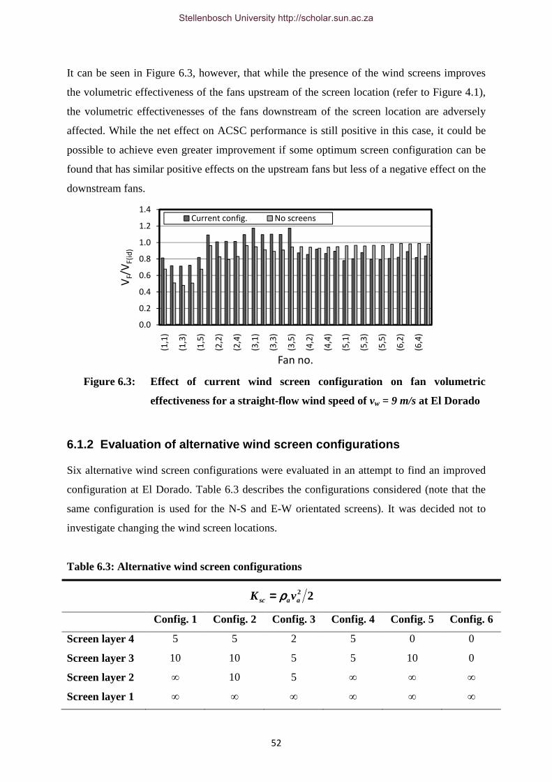
52

It can be seen in Figure 6.3, however, that while the presence of the wind screens improves

the volumetric effectiveness of the fans upstream of the screen location (refer to Figure 4.1),

the volumetric effectivenesses of the fans downstream of the screen location are adversely

affected. While the net effect on ACSC performance is still positive in this case, it could be

possible to achieve even greater improvement if some optimum screen configuration can be

found that has similar positive effects on the upstream fans but less of a negative effect on the

downstream fans.

Figure 6.3: Effect of current wind screen configuration on fan volumetric

effectiveness for a straight-flow wind speed of vw = 9 m/s at El Dorado

6.1.2 Evaluation of alternative wind screen configurations

Six alternative wind screen configurations were evaluated in an attempt to find an improved

configuration at El Dorado. Table 6.3 describes the configurations considered (note that the

same configuration is used for the N-S and E-W orientated screens). It was decided not to

investigate changing the wind screen locations.

Table 6.3: Alternative wind screen configurations

22aasc vK ρρρρ====

Config. 1 Config. 2 Config. 3 Config. 4 Config. 5 Config. 6

Screen layer 4 5 5 2 5 0 0

Screen layer 3 10 10 5 5 10 0

Screen layer 2 ∞ 10 5 ∞ ∞ ∞

Screen layer 1 ∞ ∞ ∞ ∞ ∞ ∞

0.0

0.2

0.4

0.6

0.8

1.0

1.2

1.4

(1,1

)

(1,3

)

(1,5

)

(2,2

)

(2,4

)

(3,1

)

(3,3

)

(3,5

)

(4,2

)

(4,4

)

(5,1

)

(5,3

)

(5,5

)

(6,2

)

(6,4

)

VF/

VF

(id

)

Fan no.

Current config. No screens


53

The effect of the wind screen configurations on ACSC heat transfer effectiveness is

illustrated in Figure 6.4.

(a)

(b)

Figure 6.4: Effect of alternative wind screen configuration on ACSC performance

for (a) Straight-flow, and (b) Cross-flow wind conditions

Figure 6.4 shows that it is possible to improve the ACSC performance at El Dorado through

the installation of an alternative wind screen configuration in the current wind screen

location. Configuration 6 (where high loss coefficient screens are installed to a height of

Hsc/Hi = 0.5) appears to provide the best performance in general, with performance

enhancements comparable to the other configurations at low and intermediate wind speeds

and superior performance at high wind speeds.

A comparison of the volumetric effectivenesses of the ACSC fans for the current screen

configuration and Configuration 6 is shown in Figure 6.5. It can be seen that the current wind

0.84

0.86

0.88

0.90

0.92

0.94

0.96

0.98

1.00

0 3 6 9 12

Q/Q

id

vw, m/s

Config. 1

Config. 2

Config. 3

Config. 4

Config. 5

Config. 6

Current config.

0.89

0.90

0.91

0.92

0.93

0.94

0.95

0.96

0.97

0.98

0.99

0 3 6 9 12

Q/Q

id

vw, m/s

Config. 1

Config. 2

Config. 3

Config. 4

Config. 5

Config. 6

Current config.

pa = 94800 N/m2

Ta = 19.44 °C

Tv = 43.95 °C

pa = 94800 N/m2

Ta = 19.44 °C

Tv = 43.95 °C


54

screen configuration has a larger positive effect on the performance of the fans upstream of

the wind screen location. This is to be expected since the current configuration provides a

greater obstruction to the flow under the ACSC and as such has a more significant stagnation

effect. The superior performance of Configuration 6 is as a result of the improved

performance of the fans downstream of the wind screen location. This is caused by a

reduction of the choking effect of the wind screens on the downstream fans brought about by

the removal of the screens in Screen layers 3 and 4.

Figure 6.5: A comparison of the effect of an alternative wind screen configuration

on ACSC fan performance at El Dorado

It appears that an improved wind screen configuration has been identified in the form of

Configuration 6. It was hypothesized that reducing the wind screen loss coefficient in this

configuration may result in further ACSC performance improvement. The results of an

investigation into the effect of the wind screen loss coefficient on ACSC performance,

illustrated in Figure 6.6, indicate that an optimum loss coefficient exists in the range 5 ≤ Ksc ≤

10 for Screen Configuration 6. For vw = 9 m/s the optimum lies closer to Ksc = 10. Since

ACSC performance is most severely affected at high wind speeds, Ksc = 10 was selected as

the optimum wind screen loss coefficient for Configuration 6.

0.0

0.2

0.4

0.6

0.8

1.0

1.2

1.4

(1,1

)

(1,3

)

(1,5

)

(2,2

)

(2,4

)

(3,1

)

(3,3

)

(3,5

)

(4,2

)

(4,4

)

(5,1

)

(5,3

)

(5,5

)

(6,2

)

(6,4

)

VF/

VF

(id

)

Fan no.

Current config. Config. 6

pa = 94800 N/m2

Ta = 19.44 °C

Tv = 43.95 °C


55

(a)

(b)

Figure 6.6: Effect of wind screen loss coefficient on ACSC performance under (a)

Straight-flow, and (b) Cross-flow wind conditions for Screen

Configuration 6

The question now remains whether the wind screen height, Hsc/Hi = 0.5, remains the

optimum height if the screen loss coefficient is reduced to Ksc = 10. Figure 6.7 shows the

results of an investigation into the effect of wind screen height on ACSC performance for a

screen loss coefficient of Ksc = 10, and indicates that Hsc/Hi = 0.5 remains the optimum

screen height.

0.84

0.86

0.88

0.90

0.92

0.94

0.96

0.98

1.00

0 5 10 15 20

Q/Q

id

Ksc

vw = 3 m/s

vw = 6 m/s

vw = 9 m/s

0.84

0.86

0.88

0.90

0.92

0.94

0.96

0.98

1.00

0 5 10 15 20

Q/Q

id

Ksc

vw = 3 m/s

vw = 6 m/s

vw = 9 m/s

pa = 94800 N/m2

Ta = 19.44 °C

Tv = 43.95 °C

pa = 94800 N/m2

Ta = 19.44 °C

Tv = 43.95 °C


56

Figure 6.7: Effect of wind screen height on ACSC performance for Ksc = 10 under

straight-flow wind conditions

6.2 Walkways

The effect of the addition of solid walkways on ACSC performance under windy conditions

has been investigated in previous studies. Salta and Kröger (1994) recommend the addition of

a solid walkway along the periphery of the fan platform, with a width in the range 0.159 ≤

Lw/dF ≤ 0.476 (where Lw is the walkway width), based on experimental data. Bredell (2006)

numerically investigated the effect of a solid walkway (Lw/dF = 0.333) on fan performance in

an ACSC and predicts a significant improvement in the performance of the edge fans under

windy conditions.

El Dorado has solid walkways, of width Lw/dF = 0.12, installed along the periphery of the fan

platform. It was therefore decided not to investigate walkways as a wind mitigation measure

at El Dorado. The use of walkways as a means of reducing the negative effects of wind on

ACSC performance, however, remains an interesting topic and will be investigated here using

the generic ACSC.

Bredell (2006) deduced that the installation of walkways along the periphery of the fan

platform results in increased flow rates through the edge fans as a result of a reduction in the

cross-flow velocity and abatement of the separation or distortion that occurs at the inlet of

these fans. Figure 6.8 illustrates the effect of a solid walkway of width Lw/dF = 0.29 on the

0.82

0.84

0.86

0.88

0.90

0.92

0.94

0.96

0.98

1.00

0.00 0.25 0.50 0.75 1.00

Q/Q

id

Hsc/Hi

vw = 3 m/s

vw = 6 m/s

vw = 9 m/s

pa = 94800 N/m2

Ta = 19.44 °C

Tv = 43.95 °C


57

static pressure distribution below the ACSC fan platform for a straight-flow wind speed of vw

= 9 m/s. The walkway appears to shift the low pressure region associated with separation, or

distorted flow, further upstream. A smaller portion of the upstream fan row is therefore

exposed to the distorted inflow conditions, resulting in improved performance at these fans

relative to the no walkway case.

(a) (b)

Figure 6.8: Static pressure distribution below the fan platform (a) With no

walkway present, and (b) With a solid walkway present (Lw/dF = 0.29);

for a straight-flow wind of vw = 9 m/s

While it is clear that the addition of a solid walkway along the periphery of the fan platform

is valuable, some questions regarding optimum walkway width remain. The effect of

walkway width on ACSC performance under windy conditions was subsequently

investigated. The results illustrated in Figure 6.9 indicate that ACSC performance under

windy conditions increases with walkway width but that the gain in ACSC performance per

unit walkway width increase diminishes as the width increases.


58

Figure 6.9: Effect of walkway width on ACSC performance under windy

conditions for the generic ACSC

6.3 Increasing fan power

Since the ACSC heat transfer rate is directly proportional to the mass flow rate of air through

the finned tube heat exchanger, it is possible to improve ACSC performance during periods

of strong winds and/or high ambient temperatures by increasing the mass flow rate through

the fans. One way of achieving this is to increase the fan power. However, while increasing

fan power may result in improved ACSC and steam turbine performance under unfavourable

operating conditions, the additional fan power required must be compared to the gain

associated with the improved turbine performance in order to determine the net benefit of this

method. The value of increasing fan power, as a method to improve net steam turbine power

output under windy conditions, at El Dorado will be investigated here.

The effects of increasing the power of all the ACSC fans, hereafter referred to as the “all

fans” case, as well as the effects of increasing the power of only the periphery fans, as

suggested by Liu et al. (2008) and hereafter referred to as the “periphery fans” case, were

investigated. Fan power increases of 5%, 12.5%, 20%, 30% and 40% were considered.

New fan performance characteristics were generated for the increased fan power cases based

on the design fan performance characteristic and the fan laws, as given in Kröger (2004) and

presented in equations (6.1) - (6.4).

0.80

0.82

0.84

0.86

0.88

0.90

0.92

0.94

0.96

0.98

1.00

0.0 0.1 0.2 0.3 0.4 0.5

Q/Q

id

Lw/dF

vw = 3 m/s

vw = 6 m/s

vw = 9 m/s

pa = 94800 N/m2

Ta = 19.44 °C

Tv = 43.95 °C


59

=

ad

a

Fd

F

Fd

F

N

N

P

P

ρρ

3

(6.1)

=

∆∆

ad

a

Fd

F

Fsd

Fs

N

N

p

p

ρρ

2

(6.2)

Fd

F

ad

a

N

N

V

V= (6.3)

FdF ηη = (6.4)

In equations (6.1) to (6.4) NF and NFd are the fan rotational speed at the increased fan power

and the design power respectively. PF is the increased fan power, while PFd is the design fan

power. The same applies for the fan static pressure ∆pFs, volume flow rate Va, and static

efficiency ηF. The actual and design air densities are ρa and ρad respectively.

Figure 6.10 shows how increasing fan power results in decreased turbine backpressure and

subsequently improved turbine efficiency. While this is expected, it remains to be proven

whether or not increasing fan power results in a net plant power output gain.

In order to determine the net plant power output gain/loss it is necessary to know the

relationship between the steam turbine power output and backpressure. In the absence of this

information for the turbine used at El Dorado, the turbine characteristic illustrated in Figure

6.11 was used. This curve is typical of a steam turbine selected for use in a combined-cycle

power plant with an ACSC (EPRI, 2005). It must therefore be noted that the results presented

hereafter are not accurate for El Dorado but should, none the less, give some indication of the

value of increasing fan power as a means of improving steam turbine performance under

windy conditions.


60

(a)

(b)

Figure 6.10: Effect of increasing fan power on steam turbine backpressure under

straight-flow wind conditions (a) All fans case, and (b) Periphery fans

case

Figure 6.11: Typical relationship between steam turbine power output and

backpressure in a combined-cycle power plant with an ACSC

7500

8000

8500

9000

9500

10000

10500

11000

11500

12000

0 3 6 9 12

pv,

N/m

2

vw, m/s

Original

5%

12.5%

20%

30%

40%

7500

8000

8500

9000

9500

10000

10500

11000

11500

12000

0 3 6 9 12

pv,

N/m

2

vw, m/s

Original

5%

12.5%

20%

30%

40%

-15

-10

-5

0

5

0 5000 10000 15000 20000 25000Co

rre

ctio

n t

o t

urb

ine

po

we

r o

utp

ut,

%

pv, N/m2


61

Using the gradient of the near linear portion of the curve illustrated in Figure 6.11, in the

range 8500 N/m2 < pv < 24000 N/m2 it is possible to determine the percentage change in

turbine output per unit backpressure change. The data presented in Figure 6.10 can now be

used to determine the turbine output increase associated with increasing fan power.

The power required by the fan motors is calculated as illustrated in equation (6.5). It is

assumed that the fan drive and gear box efficiencies are equal to unity.

FaFsF VpP η∆= (6.5)

The net plant power output gain, ∆Pnet, is calculated as shown in equation (6.6),

( )%100

)(

6

1

6

1

5

1)(

5

1)()()(

×

−−−

=∆∑ ∑∑∑

= = ==

origst

i i jorigFij

jadjFijorigstadjst

net P

PPPP

P (6.6)

where Pst(orig) and Pst(adj) are the steam turbine outputs for the original case (no adjustment to

fan power) and the increased fan power case respectively, while PFij(orig) and PFij(adj) are

respectively the fan power consumptions of fan (i,j) for the original and increased fan power

cases. The predicted net output gains are illustrated in Figure 6.12 for straight-flow wind

conditions.

The results presented in Figure 6.12 indicate that at high wind speeds (vw > 6 m/s) increasing

the power of all the fans by approximately 20% provides a maximised net turbine output.

Increasing the fan power by more than 20% is not justifiable since the net output gain,

although still positive, begins to diminish as a result of the large amount of power consumed

by the fans. A fan power increase in the region of 20% should also be readily achievable

without having to change the fan motors since most motors are designed with some reserve

capacity. A maximum net plant power output increase of approximately 0.12% is predicted.


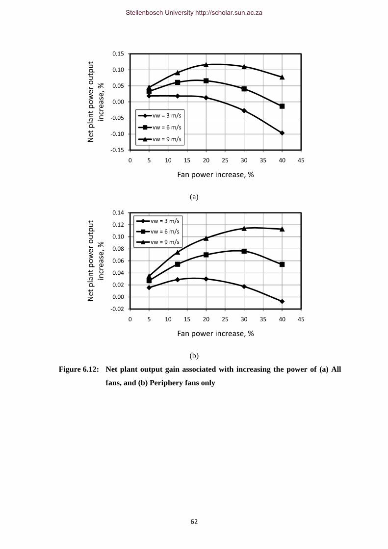
62

(a)

(b)

Figure 6.12: Net plant output gain associated with increasing the power of (a) All

fans, and (b) Periphery fans only

-0.15

-0.10

-0.05

0.00

0.05

0.10

0.15

0 5 10 15 20 25 30 35 40 45

Ne

t p

lan

t p

ow

er

ou

tpu

t

incr

ea

se,

%

Fan power increase, %

vw = 3 m/s

vw = 6 m/s

vw = 9 m/s

-0.02

0.00

0.02

0.04

0.06

0.08

0.10

0.12

0.14

0 5 10 15 20 25 30 35 40 45

Ne

t p

lan

t p

ow

er

ou

tpu

t

incr

ea

se,

%

Fan power increase, %

vw = 3 m/s

vw = 6 m/s

vw = 9 m/s


63

7. Conclusion

The objective of this study was to develop an accurate and efficient way of modelling, and

subsequently evaluating, ACSC performance using CFD. A suitable numerical model could

then be used to evaluate the performance of a specific ACSC under windy conditions in an

attempt to identify the causes of any wind induced heat transfer rate reductions. Finally, the

model could be used to evaluate the effect of certain wind effect mitigation measures on

ACSC performance.

7.1 The development of an accurate and efficient numerical

ACSC model

In order to achieve these objectives an iterative two-step modelling approach was adopted

whereby the numerical ACSC modelling was divided into global flow field and detailed

ACSC modelling stages. This approach allows for larger ACSC installations to be modelled

with relatively limited computational resources. Furthermore, the pressure jump fan model

was used to further reduce the computational expense of the ACSC performance evaluation

simulations.

A comparison of numerical results to test data was used to evaluate the accuracy of the

numerical ACSC model developed in this study. The test data was collected during the full

scale testing of El Dorado's ACSC carried out in September 2007. Good correlation was

achieved between the numerical results and test data for a number of operating points.

Discrepancies in the results, although small, can be attributed to instabilities in the ambient

conditions over the test periods considered as well as numerical inaccuracies arising from the

use of the pressure jump fan model, two step modelling approach, and other modelling

assumptions. Nonetheless, the numerical model was able to predict the actual steam turbine

backpressure to within a few percent of its measured value over each of the test periods (a

3.4% under prediction of the backpressure, corresponding to a 0.74°C discrepancy in the

turbine exhaust temperature, being the greatest discrepancy).

The numerical results were also compared to the results presented by Van Rooyen (2008) as

an additional model accuracy evaluation exercise. Van Rooyen (2008) investigated wind

effects on fan performance in the generic ACSC considered in this study. A strong correlation


64

between the predicted fan performances in the two studies was achieved for most of the fans.

However, discrepancies existed for the upstream fans. These discrepancies are thought to

have three possible sources. Firstly, Van Rooyen (2008) uses the actuator disk fan model

whereas this study employed the pressure jump method. Since the upstream fans are most

severely impacted by inlet flow distortions caused by windy conditions, it is here that any

inadequacies in the fan models will be most prevalent. It has been shown that the actuator

disk model deviates from true fan behaviour under severely distorted inflow conditions

(Thiart and von Backström, 1993) while the pressure jump method is said to provide limited

accuracy under similar conditions (Van der Spuy et al., 2009). Neither fan model appears to

be suited to modelling fan performance at the upstream fans and one model can therefore not

be recommended above the other with confidence. The second cause of discrepancy between

the results is that Van Rooyen (2008) used a two-step modelling approach without

implementing an iterative procedure. This study found that at least a single global-to-detailed

model iteration is necessary. Subsequent to the publication of his results, Van Rooyen applied

the iterative solution procedure and predicted upstream fan performances that illustrate

improved correlation with the results of this study. The third possible source of discrepancy is

that Van Rooyen (2008) only modelled a single fan at a time in his detailed ACSC model.

The influence of the remaining ACSC fans was accounted for using a uniform velocity

inlet/outlet boundary similar to that used in the global-flow-field model. This study illustrated

that the fan flow rates differ depending on the fan unit location in the ACSC. The effect of

this flow rate maldistribution on the flow field in the vicinity, and subsequently the

performance, of the fan under investigation is therefore not accounted for. Despite the

discrepancies in the predicted performances of the upstream fans the overall heat transfer

effectivenesses showed a strong correlation.

The strong correlation of the numerical results with previous numerical work and, more

importantly, with test data instils confidence in the accuracy of the results and the suitability

of the modelling method for use as an efficient ACSC performance evaluation tool.

7.2 ACSC performance under windy conditions

The results of an evaluation of El Dorado's ACSC under windy conditions identified reduced

fan performance due to distorted flow at the fan inlets, particularly those in the windward fan

rows, and hot plume recirculation as contributors to the reduction in ACSC heat transfer rate


65

associated with these conditions. These findings are consistent with literature relating to

ACSC performance reductions under windy conditions (Duvenhage and Kröger, 1996).

It was further shown that reduced fan performance has a more significant impact on reduced

ACSC heat transfer rates than plume recirculation at El Dorado. This finding is also

supported by current literature (Maulbetsch, 2008). Despite this, many studies (Liu et al.,

2009 for example) have focused on the mitigation of hot plume recirculation in an attempt to

improve ACSC performance under windy conditions. It is clear from the findings of this

study, however, that in this case greater ACSC performance enhancement potential lies in the

mitigation of reduced fan performance under windy conditions. This topic therefore formed

the focus of the wind effect mitigation measure evaluation portion of this study. It must

however be stressed that the magnitude of the contribution of hot plume recirculation and

reduced fan performance to the ACSC performance reduction under windy conditions will be

influenced by the ACSC size, geometry and the wind direction.

It was also found that the presence of wind screens at El Dorado, while appearing to have a

positive effect on the performance of the fans immediately upstream of the screen location,

seemed to reduce the performance of the downstream fans. The identification of an optimum

wind screen configuration that improves the performance of the upstream fans without being

detrimental to the performance of the downstream fans was identified as a topic for further

investigation.

7.3 Evaluation of wind mitigation measures

7.3.1 Wind screens

It was found that the installation of wind screens, in any configuration, was always beneficial

to the performance of the fans upstream of the screen location but could be detrimental to the

performance of the fans located downstream of the screen location. The magnitude of the

upstream fan performance increase was sufficient that the net effect on ACSC heat transfer

rate under windy conditions was positive for all screen configurations considered at El

Dorado (relative to the case where no screens are present). It made sense, however, that some

wind screen configuration must exist that provides the best overall performance. This would

be achieved by a screen configuration that created a significant enough stagnation effect


66

under the ACSC fan platform to benefit the upstream fans measurably without providing too

large an obstruction to the flow under the ACSC and effectively suffocating the downstream

fans.

A screen configuration consisting of medium loss coefficient screens, Ksc = 10 in this case,

installed to a height of Hsc/Hi = 0.5 was identified as an improved wind screen configuration

for El Dorado. The screens provided a large enough obstruction to the flow under the ACSC

to create a stagnation effect that benefited the upstream fans. On the other hand, the open

space immediately below the fan platform and the use of a medium loss coefficient wind

screen material allows for sufficient flow so as not to restrict the flow to the downstream

fans.

This screen configuration is also attractive from an economic point of view. It requires no

structural modification to the ACSC since the current wind screen location at El Dorado was

not altered. Also, the new configuration requires less screen material than the current

configuration and so future replacements of the screens will be cheaper. Finally, the new

screen configuration is easier to maintain and clean since it doesn't extend to the full fan

platform height.

7.3.2 Walkways

The installation of solid walkways along the ACSC periphery was shown to improve the

performance of the edge fans, and subsequently the ACSC heat transfer rate, under windy

conditions. It was also shown that increasing the width of the walkway has a positive

influence on ACSC performance. The gain per unit walkway width increase, however,

declines as the width increases. The selection of an appropriate walkway width depends on a

combination of the ACSC geometry and prevailing wind conditions. The results of this study

indicate the optimum walkway width increases with increasing wind speed and as such

ACSCs operating in high wind regions would benefit from installing wider walkways. The

installation of walkways is recommended for all ACSCs while the choice of walkway width

should be based on an appropriate lifecycle cost analysis.


67

7.3.3 Increasing fan power

Increasing the fan power was investigated as a means of improving ACSC performance

during windy periods by increasing the flow rate though the heat exchanger bundles. ACSC

fans are typically installed with some reserve capacity over and above their rated power and

so can be operated at higher powers safely without the need to install new, more powerful fan

motors. At El Dorado, the problematic high prevailing wind speed period is also in summer.

ACSC fans are typically specified based on a design air density associated with a specific

design ambient temperature. In this case the design ambient temperature is lower than the

average summer temperature and as such, according to the fan law presented in equation

(6.1), the fan power in summer will be less than the design fan power. It follows that even

more reserve power becomes available during the periods when it would be required most.

The results indicated that increasing the fan power by anything up to approximately 20%

above rated can result in net plant power output gains, relative to the design fan power case,

under windy conditions. The output gains are, however, predicted to be very small and this

method is therefore not recommended for existing ACSCs with fixed speed fan motors

already installed. The installation of variable speed motors on new ACSC installations may

be justifiable in some cases.

It must be noted however that a number of approximations were made in this analysis and

that the true value, or lack thereof, of this wind effect mitigation strategy should be evaluated

with accurate steam turbine data for a specific ACSC installation.

7.4 Importance of this study

Due to their scale, ACSCs are difficult and expensive to investigate experimentally.

Furthermore, due to the dynamic relationship between ACSC performance and ambient

conditions, analytical investigations are able to provide only limited accuracy. The numerical

ACSC modelling method developed in this study allows for the accurate and efficient

evaluation of ACSC performance under a variety of ambient conditions.

This modelling method has the potential to allow for the relatively quick and easy evaluation

of novel means of mitigating the negative impact of certain ambient conditions (wind in this


68

study) on ACSC performance. Due to the relative ease with which models can be generated,

engineers have the freedom to investigate a larger variety of possible performance enhancing

strategies than with traditional build-and-test methods (Kelecy, 2000). This fact, coupled with

the fact that the consequences of a failed attempt at identifying a successful performance

enhancing measure are negligible, means that engineers are able to experiment in a creative

and innovative manner. The potential for identifying novel and attractive ways of enhancing

ACSC performance under certain ambient conditions is therefore increased.


69

References

Air-Cooled Condenser Design, Specification, and Operation Guidelines. EPRI, Palo Alto,

CA: 2005, 1007688.

Barker, B., Running Dry at the Power Plant, EPRI Summer Journal, pp 26 – 35, 2007.

Bredell, J., Numerical Investigation of Fan Performance in a Forced Draft Air-cooled Steam

Condenser, MScEng Thesis, Department of Mechanical Engineering, University of

Stellenbosch, 2005.

Bredell, J.R., Kröger, D.G., Thiart, G.D., Numerical investigation of fan performance in a

forced draft air-cooled steam condenser, Applied Thermal Engineering, Vol. 26, pp 846 –

852, 2006.

British Standards Institution, Fans for General Purposes, Part 1, Methods for Testing

Performance, BS 848, 1997.

Carney, B., Feeley, T.J., McNemar, A., NETL Power Plant Water Research Program, US

Department of Energy, Presentation: EPRI workshop on Advanced Thermoelectric Cooling

Technologies, Charlotte, 2008.

Comparison of Alternate Cooling Technologies for U. S. Power Plants: Economic,

Environmental, and Other Tradeoffs, EPRI, Palo Alto, CA: 2004. 1005358.

DiFilippo M., Reclaiming Water for Cooling at SCE’s Mountainview Power Plant,

Presentation: EPRI workshop on Advanced Thermoelectric Cooling Technologies, Charlotte,

2008.

Duvenhage, K., Kröger, D.G., The influence of wind on the performance of forced draft air-

cooled heat exchangers, Journal of Wind Engineering and Industrial Aerodynamics, Vol. 62,

pp 259 - 277, 1996.


70

Duvenhage, K., Vermeulen, J.A., Meyer, C.J., Kröger, D.G., Flow distortions at the fan inlet

of forced-draft air-cooled heat exchangers, Applied Thermal Engineering, Vol. 16, pp 741 –

752, 1996.

FLUENT 6.3 User’s Guide, Fluent Inc., Lebanon, 2006.

Gadhamshetty, V., Nirmalakhandan, N., Myint, M., Ricketts, C., Improving Air-cooled

Condenser Performance in Combined Cycle Power Plants, Journal of Energy Engineering,

Vol. 132, No. 2, pp 81 – 88, 2006.

Hassani, V., Dickens, J., Bell, K., The Fin-on-plate Heat Exchanger: A New Configuration

for Air-cooled Power Plants, Transactions – Geothermal Resources Council, Vol. 27, pp 583

– 586, 2003.

Hightower, M., Energy and Water: Issues, Trends and Challenges, Sandia National

Laboratories, Presentation: EPRI workshop on Advanced Thermoelectric Cooling


Hotchkiss, P.J., Meyer, C.J., von Backström, T.W., Numerical investigation into the effect of

cross-flow on the performance of axial flow fans in forced draft air-cooled heat exchangers,

Applied Thermal Engineering, Vol. 26, pp 200 – 208, 2006.

Kelecy, F., Study demonstrates that simulation can accurately predict fan performance,

Journal Articles by FLUENT Software Users, JA108, 2000.

Kröger, D.G., Air-cooled heat exchangers and cooling towers, Penwell Corp., Tulsa, OK.,

2004.

Launder, B.E., Spalding, D.B., The numerical computation of turbulent flows, Computer

Methods in Applied Mechanics and Engineering, Vol. 3, Issue 2, pp 269 – 289, 1974.

Liu, P., Duan, H., Zhao, W., Numerical investigation of hot air recirculation of air-cooled

condensers at a large power plant, Applied Thermal Engineering, Vol. 29, pp 1927 – 1934,

2009.


71

Maulbetsch, J., Cooling Systems: Some things that might work, Presentation: EPRI workshop

on Advanced Thermoelectric Cooling Technologies, Charlotte, 2008.

Maulbetsch, J.S., DiFilippo, M.N., Effects of wind on air-cooled condenser performance,

Cooling Technology Institute, Paper no. TP07-04, 2007.

McGowan, C., Zammit, K., Maulbetsch, J., Field Testing of Wind Effects on Air-cooled

Condensers, Presentation: EPRI workshop on Advanced Thermoelectric Cooling


Meyer, C.J., Kröger, D.G., Numerical investigation of the effect of fan performance on forced

draft air-cooled heat exchanger plenum chamber aerodynamic behaviour, Applied Thermal

Engineering, Vol. 24, pp 359 – 371, 2004.

Meyer, C.J., Numerical investigation of the effect of inflow distortions on forced draft air-

cooled heat exchanger performance, Applied Thermal Engineering, Vol. 25, pp 1634 – 1649,

2005.

Mills, W., Potential Impacts of Climate Change on Water Resources, and Implications for

Power Plant Operations, Presentation: EPRI workshop on Advanced Thermoelectric Cooling


Owen, M.T.F., Performance evaluation of an air-cooled steam condenser, BEng Thesis,

Department of Mechanical Engineering, University of Stellenbosch, 2007.

Patankar, S.V., Numerical heat transfer, McGraw-Hill, New York, 1980.

Salta, C.A., Kröger, D.G., Effect of inlet flow distortions on fan performance in forced draft

air-cooled heat exchangers, Heat Recovery Systems and CHP, Vol. 15, No. 6, pp 555 – 561,

1995.

Shih, T., Liou, W., Shabbir, A., Yang, Z., Zhu, J., A new k-ε eddy viscosity model for high

Reynolds number turbulent flows, Computers Fluids, Vol. 24, No. 3, pp 227 – 238, 1995.


72

Stinnes, W.H., von Backström, T.W., Effect of cross-flow on the performance of air-cooled

heat exchanger fans, Applied Thermal Engineering, Vol. 22, pp 1403 – 1415, 2002.

Thiart, G.D., von Backström, T.W., Numerical simulation of the flow field near an axial flow

fan operating under distorted inflow conditions, Journal of Wind Engineering and Industrial

Aerodynamics, Vol. 45, pp 189 – 214, 1993.

Turnage, J., Water Scarcity and Power Generation: A Perspective on a Societal Issue,

UniStar Nuclear, Presentation: EPRI workshop on Advanced Thermoelectric Cooling


Van Aarde, D.J. and Kröger, D.G., Vloeiverliese deur `n A-Raam Vinbuisbundel in `n

Lugverkoelde Kondensator, MScEng Thesis, Department of Mechanical Engineering,

University of Stellenbosch, 1990.

Van der Spuy, S.J., von Backström, T.W., Kröger, D.G., Performance of low noise fans in

power plant air-cooled steam condensers, Noise Control Engineering, J.57(4), July – August,

2009.

Van Rooyen, J.A., Kröger, D.G., Performance trends of an air-cooled steam condenser under

windy conditions, Journal of Engineering for Gas Turbines and Power, Vol. 130, March 2008.

Versteeg, H.K., Malalasekera, W., An introduction to computational fluid dynamics: The

finite volume method, Pearson Education Limited, Second edition, 2007.

Wurtz, W., Nagel, P., Air cooled condensers: Application and innovative designs for today’s

power plants, Power-gen International, Orlando, Florida, 2006.


73

Appendix A - System specifications

A.1 Finned tube heat exchanger

The geometric, heat transfer and flow resistance specifications of the finned tube bundles

used in the finned tube heat exchangers for the generic ACSC are listed here.

Table A.1: Finned tube heat exchanger specifications (generic ACSC)

Description Symbol Value Units

Number of heat exchanger bundles above one

fan

nb 8

Effective frontal area of one bundle Afr 27.434 m2

Finned tube length Lt 9.55 m

Tube hydraulic diameter dh 0.02975 m

Inside area of tube per unit length Ati 0.21341 m

Inside cross sectional tube area Ats 0.00159 m2

Inside tube height Ht 0.097 m

Inside tube width Wt 0.017 m

Number of finned tube rows nr 2

Number of finned tubes per bundle in the first

row

ntb1 57

Number of finned tubes per bundle in the

second row

ntb2 58

Number of vapor passes nvp 1

Heat exchanger half apex angle θ 28 °

Ratio of minimum to free stream flow area

through the finned tube bundle

σ 0.41

Ratio of minimum to free stream flow area at

the inlet of finned tube bundle

σ21 0.86

The characteristic heat transfer parameters through the first and second tube rows at the

generic ACSC are described by equations (A.1) and (A.2) respectively, while the heat


74

exchanger loss coefficient under normal isothermal flow conditions is described by equation

(A.3).

433256.0)(1 007945.366 RyNy Gen = (A.1)

470373.0)(2 588007.360 RyNy Gen = (A.2)

43927.0)( 831.4464 −= RyK Genhe (A.3)

In equations (A.1) - (A.3),

frbaa AnmRy µ= (A.4)

A.2 Axial flow fan

The supplier fan specifications are detailed in this section. Figure A.1 illustrates the fan

dimensions for reference purposes.

Figure A.1: Fan dimensions

dh

Inlet screen

Supports

dF

xso

xsi Xbi

Xbo

Hh

Hb rb

Fan motor

Internal service grid


75

Table A.2: Axial flow fan specifications (generic ACSC)

Description Symbol Value Units

Fan diameter dF 9.145 m

Fan casing diameter dc 9.17 m

Hub/tip ratio dh/dF 0.4

Ratio of hub height to fan diameter Hh/dF 0.1

Height of inlet shroud Hb 1.92 m

Inlet shroud radius rb 1.16 m

Number of blades Nbl 8

Blade angle ψ 34.5 °

Rotational speed N 125 rpm

Inlet screen distance from fan blade

(upstream)

xsi 1.3 m

Support beam distance from fan blade

(upstream)

xbi 1.34 m

Support beam distance from fan blade

(downstream)

xbo 0.53 m

Walkway distance from fan blade

(downstream)

xso 1 m

Ratio of inlet screen area to fan casing area σsi 0.125

Ratio of support beam area to fan casing area

(upstream)

σbi 0.15

Ratio of support beam area to fan casing area

(downstream)

σbo 0.05

Ratio of walkway area to fan casing area σso 0.1

The fan static pressure characteristic for the generic ACSC fans is illustrated in equation

(A.5).

23724)( ,1014.8103515.62975.00452.320 mNVVVp aaaGenFs

−− ×−×+−=∆ (A.5)


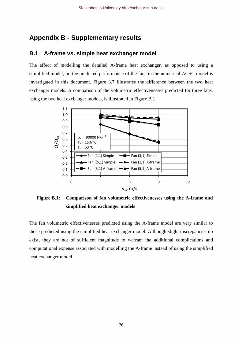
76

Appendix B - Supplementary results

B.1 A-frame vs. simple heat exchanger model

The effect of modelling the detailed A-frame heat exchanger, as opposed to using a

simplified model, on the predicted performance of the fans in the numerical ACSC model is

investigated in this document. Figure 3.7 illustrates the difference between the two heat

exchanger models. A comparison of the volumetric effectivenesses predicted for three fans,

using the two heat exchanger models, is illustrated in Figure B.1.

Figure B.1: Comparison of fan volumetric effectivenesses using the A-frame and

simplified heat exchanger models

The fan volumetric effectivenesses predicted using the A-frame model are very similar to

those predicted using the simplified heat exchanger model. Although slight discrepancies do

exist, they are not of sufficient magnitude to warrant the additional complications and

computational expense associated with modelling the A-frame instead of using the simplified

heat exchanger model.

0.0

0.1

0.2

0.3

0.4

0.5

0.6

0.7

0.8

0.9

1.0

1.1

0 3 6 9 12

Q/Q

id

vw, m/s

Fan (1,1) Simple Fan (3,1) Simple

Fan ((5,1) Simple Fan (1,1) A-frame

Fan (3,1) A-frame Fan (5,1) A-frame

pa = 90000 N/m2

Ta = 15.6 °C

Tv = 60 °C


77

B.2 Verification of pressure jump fan and heat exchanger models

The accuracy of the pressure jump fan model and simplified heat exchanger model is verified

through a comparison of the numerically predicted fan operating point under ideal flow

conditions (using the model described in Section 3.2.3) to the theoretically determined

operating point. The theoretical operating point is defined by the point of intersection of the

effective system resistance curve, given in equation (3.16), and the fan performance curve,

described by equations (A.8) and (A.9) for El Dorado and the generic ACSC respectively.

The determination of the theoretical operating point is illustrated in Figure B.2 for the generic

ACSC system. Table B.1 lists the theoretical and numerically predicted operating points for

both El Dorado and the generic system. A good correlation exists between the theoretical and

numerical values indicating that the pressure jump fan model and simplified heat exchanger

model are operating as desired.

Figure B.2: Theoretical determination of the fan operating point under ideal

operating conditions

Table B.1: Comparison of theoretical and numerically determined operating points

under ideal operating conditions

Theoretical operating

point, m3/s

Numerically determined

operating point, m3/s

El Dorado (ρa = 1.128 kg/m3) 595 600.177

Generic ACSC 636 637.565

0

50

100

150

200

250

300

350

400

400 500 600 700 800 900

p,

N/m

2

Va, m3/s

System resistance

Fan performance


78

Appendix C - Derivation of the fan performance

characteristic for the pressure jump fan model

When fans are tested to determine their performance characteristics; a free inlet, free outlet

(or type A) setup is typically used (Kröger, 2004). Figure C.1 shows a BS848 (British

Standards, 1997) Type A fan test facility.

Figure C.1: BS848 Type A fan test facility schematic (courtesy Bredell, 2005)

In this type of test setup, the static pressure difference is measured between the settling

chamber at (A), and the atmosphere at (C). The magnitude of this pressure difference at

different flow rates is given as the fan static pressure characteristic, ∆pFs. Since the flow in

the settling chamber is essentially stagnant, the fan static pressure characteristic actually

describes the total-to-static pressure rise across the fan.

The pressure jump fan model requires a function describing the static-to-static pressure rise

across the fan i.e. the static-to-static pressure rise between (B) and (C) in Figure C.1. The

required function is derived as shown hereafter.

tAsCFs ppp −=∆ (C.1)


79

In equation (C.1) the subscripts s and t stand for static and total respectively. Ignoring the

small pressure loss in the settling chamber,

22aasBtBtA vppp ρ+== (C.2)

where va is the velocity through the fan based on the effective fan area Ae as described in

equation (2.6).

Substituting equation (C.2) into (C.1) and rearranging yields the desired static-to-static

pressure rise function, ∆pF.

22 22aaFsaatAsCsBsCF vpvppppp ρρ +∆=+−=−=∆ (C.3)

Therefore, for the purpose of the pressure jump fan model, the fan static pressure

characteristics given in equations (A.8) and (A.9) need to be modified through the addition of

a dynamic pressure term.


80

Appendix D - System loss coefficients

D.1 Definition of losses in an ACSC system

Kröger (2004) derives equations for the major losses in an ACSC system based on extensive

experimental and theoretical research. A description of the system losses is given here along

with their appropriate equations.

The effective system loss for the entire ACSC is defined in terms of the draft equation, which

is repeated here for convenience.

+

+

+

−=∆

2

56

2

3

2

3

2

56 2222 frb

a

a

t

e

a

a

do

e

a

a

up

frb

a

a

tse An

mK

A

mK

A

mK

An

mKp

ρρρρθ (D.1)

Kts accounts for loss due to the fan platform supports while Kup and Kdo represent the losses

due to obstacles upstream and downstream of the fan respectively. The primary contributors

to the upstream losses are the fan inlet screen and its supports, while the primary downstream

obstacles are the fan drive system and the walkway. Kröger (2004) gives empirical relations

for Kup and Kdo in terms of the projected area of the obstacle and its distance from the fan.

Kθt is the total loss across the heat exchanger bundle and includes the kinetic energy losses at

the heat exchanger outlet. The equation for this loss coefficient under isothermal flow

conditions is given in equation (D.2).

odjcimm

het KKKKK ++

+−

−+= 21

sin

11

sin

1

θθθ (D.2)

Khe is the heat exchanger loss coefficient for normal isothermal flow as described by

equations (A.3) and (A.6) for El Dorado and the generic ACSC respectively. θm is the actual

mean flow incidence angle at the heat exchanger inlet and is a function of the A-frame half

apex angle θ.


81

1558.39133.00019.0 2 −+= θθθm (D.3)

Kci is the heat exchanger entrance contraction loss coefficient for normal flow and is based on

the normal approach free stream velocity. This loss coefficient is ultimately a function of the

ratio of the minimum to free stream flow area through the heat exchanger bundle, σ, and the

ratio of the minimum to free stream flow area at the bundle inlet, σ21, as shown in equations

(D.4) and (D.5).

621

521

421

321

22121

558944.3963169.5672041.2

4082743.0336651.004566493.06155417.0

σσσσσσσ

+−+

+−+=c (D.4)

211

−=

σσ c

ciK (D.5)

The kinetic energy loss at the heat exchanger outlet as a result of turbulent decay of the “jet”

of air leaving the heat exchanger bundles is referred to as the jetting loss, Kdj, and is given by

equation (D.6). The heat exchanger outlet loss, Ko, due to the final mixing process that is

responsible for smoothing the outlet velocity profile is given by equation (D.7). Figure D.1

illustrates the dimensions used in equations (D.6) and (D.7).

2

5.0

103797.3108601.536987.2

4.02

232

2893291.289188.2

+

+

−

=−− ×−×+

r

t

b

s

s

b

s

t

t

w

t

w

dj

L

Le

L

L

L

L

L

L

L

L

L

L

K

θθ

θ (D.6)

2

2

32

20187.2

202783.3

9874.193291.289188.2

+

−

+

+

−

=s

t

b

s

b

s

b

s

t

w

t

w

o L

L

L

d

L

d

L

L

L

L

L

L

K (D.7)


82

Figure D.1: Section of an array of A-frames illustrating relevant dimensions

D.2 Evaluation of loss coefficients for the generic ACSC

Based on the empirical relations presented by Kröger (2004),

6.1=tsK

28.0=upK

35.0=doK

Substituting σ = 0.41 and σ21 = 0.86 in equations (D.4) and (D.5) yields,

( ) ( ) ( )( ) ( ) ( ) 761.086.0558944.386.0963169.586.0672041.2

86.04082743.086.0336651.086.004566493.06155417.0654

32

=+−+

+−+=cσ

587.041.0

761.0112

=

−=ciK

Furthermore, with θ = 28°, Lt = 9.55 m, Lw = 0.397 m, Ls = 4.102 m, Lb = 4.924 m, Lr = 10.6

m and ds = 2.34 m, find according to equations (D.6) and (D.7),

Lr

Lw

ds

Lt

Ls Lb


83

( ) ( )

696.1

6.10

55.9

924.4

102.4

28

28

102.4

924.4

102.4

55.9

55.9

397.093291.2

55.9

397.089188.2

2

5.0

28103797.328108601.536987.2

4.02

232

=

+

+

−

=−− ×−×+e

Kdj

129.7102.4

55.9

924.42

34.20187.2

924.42

34.202783.3

9874.1924.4

102.4

55.9

397.093291.2

55.9

397.089188.2

2

2

32

=

⋅+

⋅−

+

+

−=oK

From equation (D.3) find,

( ) ( ) o91.231558.3289133.0280019.0 2 =−+=mθ

Substitution of equation (A.4) into equation (A.3), and considering for this case an ambient

temperature of Ta = 15.6 °C, yields,

43927.0

43927.0

53837.397

434.27810849.1831.4464 −

−

− =

⋅⋅×= a

ahe m

mK

The resulting total loss over the heat exchanger can now be calculated according to equation

(D.2).

232.133837.397

129.7696.1587.02191.23sin

11

91.23sin

13837.397

43927.0

43927.0

+=

++

+−

−+=

−

−

a

at

m

mKooθ

Substituting the loss coefficients determined above into equation (D.1) yields,


84

( )680601.1324

243927.0

222

108018.3101029.2

434.278085.12

232.133837.397

245.82085.12

35.0

245.82085.12

28.0

434.278085.12

6033.1

aa

aa

aaa

e

mm

mm

mmm

p

−−

−

×+×−=

⋅⋅+

+

⋅+

⋅+

⋅⋅−=∆

Since volumetric flow rate is related to mass flow rate as shown in equation (D.8), it is

possible to write the effective system resistance as a function of volumetric flow rate, as

shown in equation (D.9).

aaa mV ρ= (D.8)

( )56073.1324 103181.4104756.2 aae VVp −− ×+×−=∆ (D.9)


85

Appendix E - Derivation of the viscous and inertial loss

coefficients

Viscous and inertial loss coefficients are used in the heat exchanger model to account for the

effective resistance of the ACSC system to flow, as described in Section 3.2.2.2. The

derivation of these loss coefficients for the generic ACSC is illustrated here.

For the rectangular heat exchanger model, as shown in Figure 3.5, equation (E.1) holds.

( )yxa LLwV ×= (E.1)

Equation (D.9) can be approximated by a second order polynomial as shown in equation

(E.2).

( )( )aa

aae

VV

VVp224

56073.1324

106295.510132315.4

103181.4104756.2−−

−−

×+×−≈

×+×−=∆ (E.2)

Substitution of equation (E.1) into equation (E.2), with Lx = 11.8 m and Ly = 10.56 m (see

Table 3.4), results in an expression for the effective system resistance in terms of the air

velocity through the heat exchanger.

( )( ) ( )

www

wLLwwLL

VVp

yxyx

aae

1048.74163.6

106295.510132315.4

106295.510132315.4224

224

+=

××+××=

×+×−=∆−−

−−

(E.3)

The body force acting in the z-direction of each cell in the heat exchanger model is given by

equation (E.4) for Lz = 0.2 m.

wwwLpF zez 075.35082.32 +=∆= (E.4)

The body force in the z-direction is defined by Bredell (2005) as shown in equation (E.5).


86

wwvCFz

aazz α

µρ += r

2

1 (E.5)

Since the flow is restricted to the z-direction in the heat exchanger model, wv =r in equation

(E.5). The viscous and inertial loss coefficients, Cz and 1/αz respectively, can now be

determined by comparing equations (E.4) and (E.5).

1634.59=zC 1−m

And,

2610897.11 −×= mzα


87

Appendix F - Derivation of the heat exchanger energy

source term

The derivation of the source term added to the energy equation of the flow through the heat

exchanger to account for the heat transfer between the process steam and the ambient air is

described here.

The heat transfer in the first tube row is given by,

( ) ( )11111 aivpaaaiaopaa TTcmeTTcmQ −=−= (F.1)

Equation (F.1) can be rearranged to yield an expression for the air temperature immediately

after the first tube row.

( ) 1111 1 aivao TeTeT −+= (F.2)

Similarly, for the second tube row,

( ) ( )12122 aovpaaaoaopaa TTcmeTTcmQ −=−= (F.3)

and,

( ) 1222 1 aovao TeTeT −+= (F.4)

Substitution of equation (F.2) into (F.4) results in an expression for the air temperature at the

heat exchanger exit in terms of the steam, and heat exchanger air inlet, temperatures.

( ) ( )[ ]111222 11 aivvao TeTeeTeT −+−+= (F.5)

The total heat transfer through the heat exchanger is,


88

( )1221 aiaopaa TTcmQQQ −=+= (F.6)

The energy source term to be added to the flow as it passes through the numerical heat

exchanger model is defined as,

VQSE δδ= (F.7)

Substitution of equation (F.6) into equation (F.7) yields,

( ) ( )1212 aiaopaz

aaiaopa

aE TTc

L

wTTc

V

mS −=−=

ρδδ

(F.8)


89

Appendix G - Test operating periods

The four periods selected from the test data, collected during the full scale testing of El

Dorado's ACSC (Owen, 2007), for comparison with numerical results are described in detail

here. The parameters extracted from the data for use in the numerical simulations are listed in

Table 4.2. A diagram illustrating the layout of El Dorado’s ACSC is presented in Figure G.1

for reference purposes.

Figure G.1: El Dorado ACSC layout and fan numbering scheme

Ambient temperature and wind velocity measurements were recorded at elevations of 2 m, 5

m and 11 m above ground level on a weather mast located approximately 150 m to the south

of the ACSC. Power law wind and temperature profiles of the form shown in equations (G.1)

Plant buildings

(1,1) (1,2) (1,3) (1,4) (1,5)

(2,1) (2,2) (2,3) (2,4) (2,5)

(3,1) (3,2) (3,3) (3,4) (3,5)

(4,1) (4,2) (4,3) (4,4) (4,5)

(5,1) (5,2) (5,3) (5,4) (5,5)

(6,1) (6,2) (6,3) (6,4) (6,5)

N

150 m

Weather mast


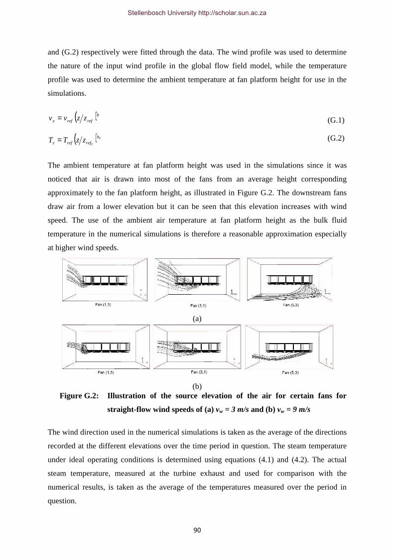
90

and (G.2) respectively were fitted through the data. The wind profile was used to determine

the nature of the input wind profile in the global flow field model, while the temperature

profile was used to determine the ambient temperature at fan platform height for use in the

simulations.

( )b

refrefz zzvv = (G.1)

( ) T

T

brefrefz zzTT = (G.2)

The ambient temperature at fan platform height was used in the simulations since it was

noticed that air is drawn into most of the fans from an average height corresponding

approximately to the fan platform height, as illustrated in Figure G.2. The downstream fans

draw air from a lower elevation but it can be seen that this elevation increases with wind

speed. The use of the ambient air temperature at fan platform height as the bulk fluid

temperature in the numerical simulations is therefore a reasonable approximation especially

at higher wind speeds.

(a)

(b) Figure G.2: Illustration of the source elevation of the air for certain fans for

straight-flow wind speeds of (a) vw = 3 m/s and (b) vw = 9 m/s

The wind direction used in the numerical simulations is taken as the average of the directions

recorded at the different elevations over the time period in question. The steam temperature

under ideal operating conditions is determined using equations (4.1) and (4.2). The actual

steam temperature, measured at the turbine exhaust and used for comparison with the

numerical results, is taken as the average of the temperatures measured over the period in

question.


91

G.1 Test period 1 (TP1)

Test period 1 is a 20 minute period between 21:37 and 21:59 on 14 September 2007.

Figure G.3: Ambient temperature data recorded for TP1

Figure G.4: Power law fit through temperature data for TP1

Figure G.5: Wind speed data recorded for TP1

29.0

29.5

30.0

30.5

31.0

31.5

21:36 21:43 21:50 21:57

T a, °

C

Time

z = 2 m z = 5 m z = 11 m

0

2

4

6

8

10

12

14

29.0 29.5 30.0 30.5 31.0 31.5

z, m

T, °C

11 m data

5 m data

2 m data

Power law fit

0.00.51.01.52.02.53.03.54.04.55.05.5

21:36 21:43 21:50 21:57

v z, m

/s

Time

z = 2 mz = 5 mz = 11 mPower law value at given elevation


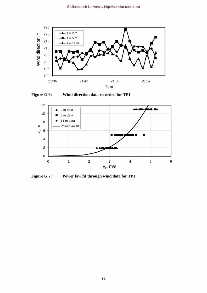
92

Figure G.6: Wind direction data recorded for TP1

Figure G.7: Power law fit through wind data for TP1

190

195

200

205

210

215

220

225

21:36 21:43 21:50 21:57

Win

d di

rect

ion,

°

Time

z = 2 m

z = 5 m

z = 11 m

0

2

4

6

8

10

12

0 1 2 3 4 5 6

z, m

vz, m/s

2 m data

5 m data

11 m data

Power law fit


93






37.6

37.8

38.0

38.2

38.4

38.6

38.8

39.0

39.2

39.4

15:12 15:15 15:18 15:21 15:24 15:27 15:30 15:33

T a, °

C

Time

z = 2 m z = 5 m z = 11 m

0

2

4

6

8

10

12

14

38.0 38.2 38.4 38.6 38.8 39.0 39.2 39.4

z, m

T, °C

z = 2 m data

z = 5 m data

z = 11 m data

Power law fit

2

3

4

5

6

7

8

9

10

11

12

13

15:12 15:15 15:18 15:21 15:24 15:27 15:30 15:33

v z, m

/s

Time



94



200

210

220

230

240

250

260

15:12 15:15 15:18 15:21 15:24 15:27 15:30 15:33

Win

d di

rect

ion,

°

Time

z = 2 m z = 5 m z = 11 m

0

2

4

6

8

10

12

0 2 4 6 8 10 12 14

z, m

vz, m/s

z = 2 m data

z = 5 m data

z = 11 m data

Power law fit


95






35.6

35.8

36.0

36.2

36.4

36.6

36.8

17:11 17:13 17:16 17:19 17:22 17:25 17:28 17:31

T, °

C

Time

z = 2 m z = 5 m z = 11 m

0

2

4

6

8

10

12

14

35.8 35.9 36 36.1 36.2 36.3 36.4 36.5

z, m

T, °C

z = 2 m data

z = 5 m data

z = 11 m data

Power law fit

3

4

5

6

7

8

9

10

17:11 17:13 17:16 17:19 17:22 17:25 17:28 17:31

v z, m

/s

Time

z = 2 mz = 5 mz = 11 m


96



220

225

230

235

240

245

250

17:11 17:13 17:16 17:19 17:22 17:25 17:28 17:31

Win

d di

rect

ion,

°

Time

z = 2 m z = 5 m z = 11 m

0

2

4

6

8

10

12

0 2 4 6 8 10

z, m

vz, m/s

z = 2 m data

z = 5 m data

z = 11 m data

Power law fit


97






32.0

32.2

32.4

32.6

32.8

33.0

33.2

33.4

33.6

17:25 17:28 17:31 17:34 17:36 17:39 17:42 17:45

T a, °

C

Time

z = 2 m z = 5 m z = 11 m

0

2

4

6

8

10

12

14

32.0 32.2 32.4 32.6 32.8 33.0 33.2 33.4 33.6

z, m

T, °C

z = 2 m data

z = 5 m data

z = 11 m data

Power law fit

2

3

4

5

6

17:25 17:28 17:31 17:34 17:36 17:39 17:42 17:45

v z, m

/s

Time



98



200

210

220

230

240

250

260

270

280

290

300

17:25 17:28 17:31 17:34 17:36 17:39 17:42 17:45

Win

d di

rect

ion,

°

Time

z = 2 m z = 5 m z = 11 m

0

2

4

6

8

10

12

0 1 2 3 4 5 6

z, m

vz, m/s

z = 2 m data

z = 5 m data

z = 11 m data

Power law fit


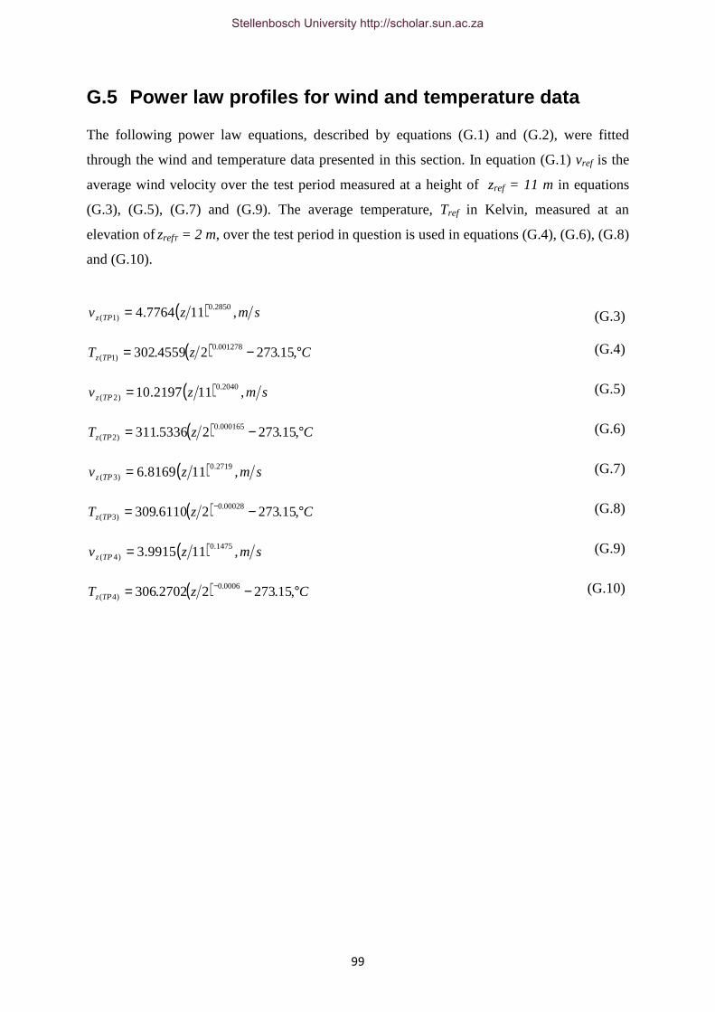
99

G.5 Power law profiles for wind and temperature data

The following power law equations, described by equations (G.1) and (G.2), were fitted

through the wind and temperature data presented in this section. In equation (G.1) vref is the

average wind velocity over the test period measured at a height of zref = 11 m in equations

(G.3), (G.5), (G.7) and (G.9). The average temperature, Tref in Kelvin, measured at an

elevation of zrefT = 2 m, over the test period in question is used in equations (G.4), (G.6), (G.8)

and (G.10).

( ) smzv TPz ,117764.4 2850.0)1( = (G.3)

( ) CzT TPz °−= ,15.27324559.302 001278.0)1(

(G.4)

( ) smzv TPz ,112197.10 2040.0)2( =

(G.5)

( ) CzT TPz °−= ,15.27325336.311 000165.0)2(

(G.6)

( ) smzv TPz ,118169.6 2719.0)3( =

(G.7)

( ) CzT TPz °−= − ,15.27326110.309 00028.0)3(

(G.8)

( ) smzv TPz ,119915.3 1475.0)4( =

(G.9)

( ) CzT TPz °−= − ,15.27322702.306 0006.0)4(

(G.10)


100

Appendix H - Wind screen material tests

The wind tunnel test setup used to determine the wind screen material loss coefficient is

illustrated in Figure H.1 and described thereafter (Kröger, 2004).

Figure H.1: Wind tunnel test setup

Air is drawn through the rounded inlet, where the drybulb temperature is measured, and

through a sample of the wind screen material at (1) under the influence of a radial fan (8).The

static pressure difference across the screen is measured at points located in the duct wall at

(2). After passing through the screen, the air moves through two sets of mixers at (3) and a

venturi in which a sampling tube is located at (4). The mixers and sampling tube are used to

allow for accurate measurement of the air temperature in this section of the wind tunnel. The

air mass flow rate is determined by measuring the static pressure drop at (7) across one or

more elliptical nozzles mounted in a plate at (6). The nozzle plate is located between two

perforated plates (5). The mass flow rate through the tunnel is given by equation (H.1).

nangna pYACm ∆= ρφ 2 (H.1)

An and ∆pn are the nozzle cross sectional area and the pressure drop across the nozzle plate

respectively. The nozzle coefficient of discharge, Cn, is a function of the nozzle Reynolds

number, Ren, as illustrated in equations (H.2) - (H.4).

For 30 000 < Ren < 100 000

101

3172127 1033514110653944103781769458030 nnnn Re.Re.Re..C −−− ×+×−×+= (H.2)

For 100 000 < Ren < 350 000

2127 10611008197580 nnn Re.Re..C −− ×−×+= (H.3)

For Ren > 350 000

9940.Cn = (H.4)

The gas expansion factor,gφ , is approximated using equation (H.5).

( )vpupng ccpp 431 ∆−=φ (H.5)

where pup is the pressure upstream of the nozzles and cp/cv = 1.4 for air.

The approach velocity factor, Y, for a compressible fluid is given by equation (H.6).

( ) ( ) ( )vpupnupnupn ccppAAAA.Y ∆++= 22 2501 (H.6)

where Aup is the area of the wind tunnel upstream of the nozzles.

The wind screen material loss coefficient is determined according to equation (H.7).

22 scascsc vpK ρ∆= (H.7)

where vsc is the flow velocity through the screen, as given by equation (H.8) where Asc is the

screen material sample cross sectional area.

scaasc Amv ρ= (H.8)

The test results for the 55% and 65% closed area screen materials are illustrated in Figure

H.2. The 90% closed area screen material behaved as a solid obstruction to the flow.

102

Figure H.2: Wind screen material loss coefficients

The screen material loss coefficients are very near to constant values and were subsequently

modelled as such to reduce the computational requirements of the analyses carried out in this

study. The average characteristic flow parameter through the screens is typically less than Ry

= 2.0 x 105 m-1 and values of Ksc = 2 and Ksc = 5 were selected for the 55% and 65% closed

area screen materials respectively.

0

1

2

3

4

5

6

7

1 2 3 4 5

Ksc

Ry x 105

55% closed area material

65% closed area material

5. ACSC performance under windy conditions

Documents

Transcript of 5. ACSC performance under windy conditions