Edited by Tommaso Cucinotta and Julio Medina

4th International Workshop onAnalysis Tools and

Methodologies for Embeddedand Real-time Systems

July 9th, 2013, Paris, France

In conjunction with:The 25th Euromicro Conference on Real-Time Systems

(ECRTS 2013)

c©Copyright 2013 by the authors

i

This page has been left intentionally blank.

Edited by Tommaso Cucinotta and Julio Medina

4th International Workshop onAnalysis Tools and

Methodologies for Embeddedand Real-time Systems

July 9th, 2013, Paris, France

In conjunction with:The 25th Euromicro Conference on Real-Time Systems

(ECRTS 2013)

c©Copyright 2013 by the authors

This page has been left intentionally blank.

WATERS 2013 i

Table of Contents

Message from the Program Chairs ii

Program Committee iv

Keynote Speech

Papyrus: an eclipse-based open source initiative for exploit-ing the full modeling power of UML and DSML’s

v

Camille Letavernier and Florian Noyrit

Session A

A Simulation Environment Based on OMNeT++ For Au-tomotive CAN–Ethernet Networks

1

Jun Matsumura, Yutaka Matsubara, Hiroaki Takada,Masaya Oi, Masumi Toyoshima and Akihito Iwai

CloudNetSim - Simulation of Real-Time Cloud ComputingApplications

7

Tommaso Cucinotta and Aram Santogidis

A Simulation Tool for Optimal Phasing of Nodes Distributedover Industrial Real-Time Networks

13

Sang-Hun Lee, Hyun-Wook Jin and Kanghee Kim

Session B

Many-in-one Response-Time Analyzer for Controller AreaNetwork

19

Saad Mubeen, Jukka Mäki-Turja and Mikael Sjödin

On the Convergence of Experimental Methodologies for Dis-tributed Systems: Where do we stand?

25

Maximiliano Geier, Lucas Nussbaum and Martin Quinson

Tropos for Embedded Real-Time Control System Modelingand Simulation

31

Nesrine Darragi, Philippe Bon, Simon Collart-Dutilleul,El-Miloudi El-Koursi

WATERS 2013 ii

Message from the Program Chairs

Real-Time schedulability analysis techniques, scheduling algorithms, and syn-chronisation protocols, have greatly evolved and continue to evolve in our researchcommunity along the last 40 years. New hardware platforms and the increasingdemand from different application domains, are posing more and more challengeson the predictability and reliability of applications in terms of their timing be-haviour. While theory grows and goes rising in complexity, the gap betweenindustrial practice and state-of-the-art research techniques keeps also enlarging,leading to a panoply of strategies, formalisms, abstraction techniques, standards,and business models to deal with the very basic problem: how to assure timingpredictability of software, and be able to build dependable systems, applications,or products upon it.

As it happens with all computer science and IT related research areas, theadoption of theoretical research results into industrial practice follows an evo-lutionary pattern, in which each formalism, paradigm or language fights for itsplace. As for many other knowledge domains, the effective means for compar-ing, evaluating and choosing among the available techniques relies on the scien-tific method; this requires experimentation and practice. Hence, software tools,methodologies, comprehensive use cases data sets, and benchmarks are the effec-tive arms to find a place in this battle against complexity.

Besides, different authors use different algorithms for generating random tasksets, different application traces when simulating dynamic real-time systems, dif-ferent simulation engines when simulating scheduling algorithms. Instead, re-search in the field of real-time and embedded systems would greatly benefit fromthe availability of well-engineered, possibly open tools, simulation frameworksand data sets which may constitute a common metrics for evaluating simulationor experimental results in the area. It would be really beneficial to have a pos-sibly wide set of reusable data sets or behavioural models coming from realisticindustrial use-cases over which to evaluate the performance of novel algorithms.Availability of such items would increase the possibility to compare novel tech-niques in dealing with problems already tackled by others from the multifacetedviewpoints of effectiveness, overhead, performance, applicability, etc.

The initial goal of this workshop was to bring visibility and recognise thework of those scientists who write software that is useful for our community; tomake these tools more widely known in it; and to create a group of researchersinterested in contributing with new software and tools.

In this fourth edition, we have enlarged the spectrum of software tools, OSservices and networking resources to domains and information technologies inwhich soft real-time requirements are dominant. As in former editions, we alsoask authors to provide their software (or links to their web page where the soft-ware is made available). All this information is available through the workshopweb page1. Also, our mailing list in Google Group is active to distribute infor-mation on the workshop themes2.

1http://www.ctr.unican.es/waters2013/2https://groups.google.com/forum/?fromgroups#!forum/ecrts-waters

WATERS 2013 iii

We would like to thank the Euromicro organisation for having allowed us toorganise this event, and particularly Laurent George, Gerhard Fohler and StefanM. Petters for their prompt and ready support. We would like to thank the Real-Time Systems Laboratory of Scuola Superiore Sant’Anna and the Computersand Real-Time Group of the University of Cantabria for their support in hostingthe WATERS website. Also, we would like to thank all the authors for havingsubmitted their work to the workshop for selection, the Program Committeemembers for their effort in reviewing the papers, the presenters for ensuringinteresting sessions, and the attendees for participating into this event.

We are sure that interesting ideas and discussions will come out of the pre-sentations, demos and the questions that will alternate along the day. We hopeyou to find this day interesting and enjoyable and your overall experience withWATERS to bring you back for more our next edition.

The WATERS 2013 Chairs

Tommaso Cucinotta3 and Julio Medina4

3Tommaso Cucinotta is with Bell Laboratories, Alcatel-Lucent, Dublin, Irelande-mail: tommaso.cucinotta@alcatel-lucent.com

4Julio Medina is with Departamento de Electrónica y Computadores Universidad deCantabria, Santander, Spaine-mail: julio.medina@unican.es

WATERS 2013 iv

Program Committee

• Luca Abeni (University of Trento, Italy)

• Ian Broster (Rapita Systems Ltd, York, UK)

• Laura Carnevali (University of Florence, Italy)

• Marisol García Valls (Universidad Carlos III de Madrid, Spain)

• Laurent George (INRIA Paris-Rocquencourt, France)

• Michael Gonzalez (Universidad de Cantabria, Spain)

• Kwei-Jay Lin (University of California, Irvine, US)

• Giuseppe Lipari (École Normale Supèrieure de Cachan, France)

• Thomas Nolte (Mälardalen University, Sweden)

• Martin Quinson (Nancy University, France)

• Simon Schliecker (Symtavision GmbH, Braunschweig, Germany)

• Thomas C. Schmidt (Hamburg University of Applied Sciences, Germany)

• Wang Yi (Uppsala University, Sweden)

Papyrus: an eclipse-based open source initiative for exploiting the full modeling power of UML and DSML's

Camille LETAVERNIER and Florian NOYRIT CEA LIST/DILS/ Laboratory of model driven engineering for embedded systems

(LISE)

The principle of separating concerns is widely used in engineering to address complexity. In Model-Driven Engineering (MDE), this principle notably led to the development of Domain Specific Modeling Languages (DSML). Those languages provide constructs that are directly aligned with the concepts of the domain in question. A specific domain, in the broad sense, can be an application domain (e.g. auto-motive) or a specific concern (e.g. requirement modeling). This coincides nicely with the vision specified in the ISO/IEC/IEEE 42010 standard which suggests that each stakeholder needs dedicated viewpoints to address his or her concerns. It is the responsibility of language designers and methodologists to provide the DSMLs that support these viewpoints. And, it is the responsibility of tool designers to provide appropriate user interfaces to corresponding language authoring tools.

This is precisely what Papyrus project provides: a modeling environment that let language designers define their DSML for a specific viewpoint and let tool designers configure the modeling environment to support the desired viewpoint. However, Papyrus provides those features under the following motto: “Don’t reinvent the wheel, adopt UML instead but tailor it to your needs”. To do that, Papyrus provides a UML profile editor to let language designer define the DSML. But, more important, Papyrus provides means to tool designers to customize the modeling environment in order to tailor the UI to corresponding viewpoint. Papyrus is therefore a generic modeling environment that can be customized to support UML-based DSML.

This talk presents the key concepts and features that are available today in Papyrus to define and implement UML-based DSMLs. It will especially show how UML-based DSML can be much more than just an extension of the UML metamodel. We will also introduce features that are coming soon together with those we plan to develop in the long term.

WATERS 2013 v

A Simulation Environment based on OMNeT++for Automotive CAN–Ethernet Networks

Jun Matsumura, Yutaka Matsubara, Hiroaki TakadaGraduate School of Information Science

Nagoya University, Aichi, Japan

Masaya Oi, Masumi Toyoshima, Akihito IwaiDENSO CORPORATION

Aichi, Japan

Abstract—Due to the rapid increase in the functionalityrequirements of automotive control networks, mixed CAN (Con-troller Area Network) and Ethernet networks have recentlygained considerable attention. This paper presents a simulationenvironment for CAN–Ethernet networks based on the open-source network simulator OMNeT++, part of the INET frame-work. We develop simulation models of CAN and a CAN–Ethernet Gateway (GW). To validate the CAN model, we mea-sure the end-to-end latency of CAN messages and compare itsperformance with an existing CAN network simulator. We applythe proposed simulation environment to an automotive CAN–Ethernet system, and confirm that it is an effective aid in thedesign and evaluation of such networks.

I. INTRODUCTION

Controller Area Network (CAN), originally developed byBosch in 1985, has long been used as the standard protocolfor automotive control networks. In recent years, because thefunctionality demands of such systems have grown rapidly, ithas become increasingly difficult to meet network requirementsusing only the CAN and Local Interconnect Network (LIN)protocols. Moreover, some new functions using Ethernet havebeen considered, such as Diagnostics on Internet Protocol(DoIP) and reprogramming the firmware of Electronic ControlUnits (ECUs). Ethernet offers the twin advantages of highcommunication speed and a flexible network topology. How-ever, its lack of a real-time property means that it has not,to date, been used in a control network. To overcome theseproblems, there has been some research into mixed CAN–Ethernet networks [4], and some CAN–Ethernet gateway (GW)products have been released [6], [7].

In order to integrate CAN–Ethernet networks early in thedevelopment process, we need to explore an appropriate designthat can meet certain stated requirements, because existingCANs cannot be reused. The requirements include the end-to-end latency of messages, the number of GWs, and the amountof buffering to be implemented in each GW. The evaluationof CAN–Ethernet networks can be conducted by analytical orsimulation methods. The worst-case response time has beenconsidered as an analytical method in CAN networks [3],[12] and Ethernet networks [8], [9]. In addition, the Symta/Sanalytical tool supports CAN–Ethernet networks [13].

Once we obtain an analytical method for a targeted net-work, it can be evaluated quickly. However, the communicationprotocol and network topology involved in developing suchanalytical methods for complex message sets is not straight-forward. Therefore, simulation methods are more effective fordesigning and evaluating the early states of a network.

To date, many network simulators have been developed,such as CANoe [11], Venet [14], OPNET [2], TrueTime [1],and OMNeT++ [5]. Provided by Vector Inc., CANoe is a well-known development tool for the design of automotive controlnetworks, and supports many network protocols, such asCAN, LIN, MOST, FlexRay, and Ethernet. OPNET (OPNETTechnologies Inc.) is a bit-level network simulator; such toolsgive more accurate simulations than message-level simulators.However, their simulation speed is generally slow. In addition,as OPNET is a commercial tool, we cannot easily add asimulation model of a new network protocol. Therefore, toevaluate the early states of a network, message-level simulatorsare more suitable than bit-level simulators. Venet, developedby InterDesign Technologies Inc., is a message-level simu-lator for CANs, but does not support the Ethernet protocol.TrueTime, distributed by Lund University and based on MAT-LAB/Simulink, is a message-level simulator that does supportEthernet, as well as MAC and CSMA/CD. However, IP andTCP/UDP are not supported. The open-source discrete timeevent simulator OMNeT++ is well-documented for both usersand model developers. This means that we can easily developa new simulation model. Although OMNeT++ supports manymultimedia communication protocols, no automotive networkprotocols are currently supported.

In this paper, we propose a simulation environment forCAN–Ethernet networks based on OMNeT++ and the INETframework [10]. We develop a CAN simulation model and aCAN–Ethernet GW model. To validate the developed CANmodel, we compare the end-to-end latency of CAN messagesusing the proposed simulator with results from the Venet tool.Furthermore, we perform a case study for an automotive CAN–Ethernet network and confirm the applicability of the proposedsimulator.

This paper is organized as follows: Section 2 presents anoverview of the proposed simulation environment, and Section3 describes in detail the simulation models for CAN and CAN–Ethernet GW. Section 4 gives the results of our evaluation ofthe developed CAN model and a case study. Finally, Section5 concludes the paper.

II. SIMULATION ENVIRONMENT

A. Overview

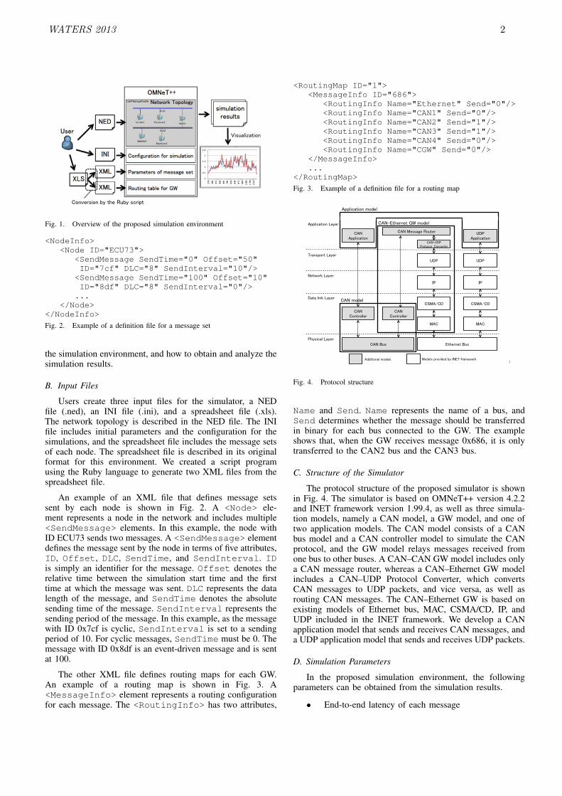
Fig. 1 shows an overview of the proposed simulationenvironment, with input files on the left, the simulator inthecenter, and the output files on the right. In the followingsections, we describe the necessary input files, an overview of

WATERS 2013 1

!"#$%&'($)*+,(-".(/012341

2341

5651

6781

936,:;;1

6,$<".=(:">"+"'?1

@"&-%'#.)$%"&(-".(A%B#+)$%"&1

A%B#+)$%"&(

.,A#+$A1

24C1D).)B,$,.A("-(B,AA)',(A,$1

EA,.1

@"&F,.A%"&(*?($G,(!#*?(AH.%>$1

I%A#)+%J)$%"&1

Fig. 1. Overview of the proposed simulation environment

<NodeInfo><Node ID="ECU73">

<SendMessage SendTime="0" Offset="50"ID="7cf" DLC="8" SendInterval="10"/>

<SendMessage SendTime="100" Offset="10"ID="8df" DLC="8" SendInterval="0"/>

...</Node>

</NodeInfo>

Fig. 2. Example of a definition file for a message set

the simulation environment, and how to obtain and analyze thesimulation results.

B. Input Files

Users create three input files for the simulator, a NEDfile (.ned), an INI file (.ini), and a spreadsheet file (.xls).The network topology is described in the NED file. The INIfile includes initial parameters and the configuration for thesimulations, and the spreadsheet file includes the message setsof each node. The spreadsheet file is described in its originalformat for this environment. We created a script programusing the Ruby language to generate two XML files from thespreadsheet file.

An example of an XML file that defines message setssent by each node is shown in Fig. 2. A <Node> ele-ment represents a node in the network and includes multiple<SendMessage> elements. In this example, the node withID ECU73 sends two messages. A <SendMessage> elementdefines the message sent by the node in terms of five attributes,ID, Offset, DLC, SendTime, and SendInterval. IDis simply an identifier for the message. Offset denotes therelative time between the simulation start time and the firsttime at which the message was sent. DLC represents the datalength of the message, and SendTime denotes the absolutesending time of the message. SendInterval represents thesending period of the message. In this example, as the messagewith ID 0x7cf is cyclic, SendInterval is set to a sendingperiod of 10. For cyclic messages, SendTime must be 0. Themessage with ID 0x8df is an event-driven message and is sentat 100.

The other XML file defines routing maps for each GW.An example of a routing map is shown in Fig. 3. A<MessageInfo> element represents a routing configurationfor each message. The <RoutingInfo> has two attributes,

<RoutingMap ID="1"><MessageInfo ID="686">

<RoutingInfo Name="Ethernet" Send="0"/><RoutingInfo Name="CAN1" Send="0"/><RoutingInfo Name="CAN2" Send="1"/><RoutingInfo Name="CAN3" Send="1"/><RoutingInfo Name="CAN4" Send="0"/><RoutingInfo Name="CGW" Send="0"/>

</MessageInfo>...

</RoutingMap>

Fig. 3. Example of a definition file for a routing map

!"#$%&'( )*+,-.,*$%&'(

/"!( /"!(

!"#(

!0.*-011,-(

!"#$/,''23,$40&*,-(

!5/"6!7(

8+9':;21$<29,-(

72*2$1:.=$<29,-(

#,*>0-=$<29,-(

?8(

@-2.'A0-*$<29,-(

B78(

"AA1:;2*:0.$<29,-(

!"#(

"AA1:;2*:0.(

B78(

"AA1:;2*:0.(

!5/"6!7(

?8(

B78(

!"#(

!0.*-011,-(

!"#C)*+,-.,*$DE$F0G,1(

/0G,1'$A-0H:G,G$I9$?#)@$J-2F,>0-=("GG:*:0.21$F0G,1'(K(

!"#CB78(

8-0*0;01$$!0.H,-*,-(

!"#$F0G,1(

"AA1:;2*:0.$F0G,1(

Fig. 4. Protocol structure

Name and Send. Name represents the name of a bus, andSend determines whether the message should be transferredin binary for each bus connected to the GW. The exampleshows that, when the GW receives message 0x686, it is onlytransferred to the CAN2 bus and the CAN3 bus.

C. Structure of the Simulator

The protocol structure of the proposed simulator is shownin Fig. 4. The simulator is based on OMNeT++ version 4.2.2and INET framework version 1.99.4, as well as three simula-tion models, namely a CAN model, a GW model, and one oftwo application models. The CAN model consists of a CANbus model and a CAN controller model to simulate the CANprotocol, and the GW model relays messages received fromone bus to other buses. A CAN–CAN GW model includes onlya CAN message router, whereas a CAN–Ethernet GW modelincludes a CAN–UDP Protocol Converter, which convertsCAN messages to UDP packets, and vice versa, as well asrouting CAN messages. The CAN–Ethernet GW is based onexisting models of Ethernet bus, MAC, CSMA/CD, IP, andUDP included in the INET framework. We develop a CANapplication model that sends and receives CAN messages, anda UDP application model that sends and receives UDP packets.

D. Simulation Parameters

In the proposed simulation environment, the followingparameters can be obtained from the simulation results.

• End-to-end latency of each message

WATERS 2013 2

!"#$%&'()&**+)$,&-+*.

/0(1$,+2234+$5677+).

!"#$388*0%3(0&'$,&-+*.

!"#$'&-+.

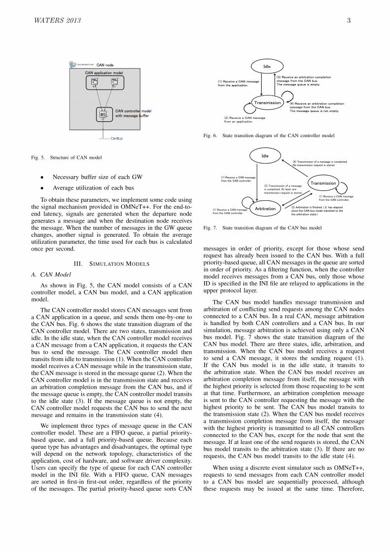
Fig. 5. Structure of CAN model

• Necessary buffer size of each GW

• Average utilization of each bus

To obtain these parameters, we implement some code usingthe signal mechanism provided in OMNeT++. For the end-to-end latency, signals are generated when the departure nodegenerates a message and when the destination node receivesthe message. When the number of messages in the GW queuechanges, another signal is generated. To obtain the averageutilization parameter, the time used for each bus is calculatedonce per second.

III. SIMULATION MODELS

A. CAN Model

As shown in Fig. 5, the CAN model consists of a CANcontroller model, a CAN bus model, and a CAN applicationmodel.

The CAN controller model stores CAN messages sent froma CAN application in a queue, and sends them one-by-one tothe CAN bus. Fig. 6 shows the state transition diagram of theCAN controller model. There are two states, transmission andidle. In the idle state, when the CAN controller model receivesa CAN message from a CAN application, it requests the CANbus to send the message. The CAN controller model thentransits from idle to transmission (1). When the CAN controllermodel receives a CAN message while in the transmission state,the CAN message is stored in the message queue (2). When theCAN controller model is in the transmission state and receivesan arbitration completion message from the CAN bus, and ifthe message queue is empty, the CAN controller model transitsto the idle state (3). If the message queue is not empty, theCAN controller model requests the CAN bus to send the nextmessage and remains in the transmission state (4).

We implement three types of message queue in the CANcontroller model. These are a FIFO queue, a partial priority-based queue, and a full priority-based queue. Because eachqueue type has advantages and disadvantages, the optimal typewill depend on the network topology, characteristics of theapplication, cost of hardware, and software driver complexity.Users can specify the type of queue for each CAN controllermodel in the INI file. With a FIFO queue, CAN messagesare sorted in first-in first-out order, regardless of the priorityof the messages. The partial priority-based queue sorts CAN

!"#$%&'&()&$*$+,-$.&//*0&$

123.$45&$*667('*4(389:

!;#$%&'&()&$*8$*2<(42*4(38$'3.67&4(38$

.&//*0&$123.$45&$+,-$<=/9$:

>5&$.&//*0&$?=&=&$(/$&.64@9:

AB7&:

>2*8/.(//(38: !C#$%&'&()&$*8$*2<(42*4(38$'3.67&4(38$

.&//*0&$123.$45&$+,-$<=/9:

>5&$.&//*0&$?=&=&$(/$834$&.64@9:

!D#$%&'&()&$*$+,-$.&//*0&$

123.$*8$*667('*4(389:

Fig. 6. State transition diagram of the CAN controller model

!"#$%&'&()&$*$+,-$.&//*0&$

123.$45&$+,-$'3642377&289

!:#$,2;(42*4(36$(/$1(6(/5&<8$!=$5*/$&7*>/&<$

/(6'&$45&$+,-$;?/$.3<&7$42*6/(4&<$43$45&$

45&$*2;(42*4(36$/4*4&8#9

@<7&9

,2;(42*4(369

!A#$B2*6/.(//(36$31$*$.&//*0&$(/$'3.>7&4&<8$

-3$42*6/.(//(36$2&C?&/4$(/$/432&<89

B2*6/.(//(369

!"#$%&'&()&$*$+,-$.&//*0&$

123.$45&$+,-$'3642377&289

!"#$%&'&()&$*$+,-$.&//*0&$

123.$45&$+,-$'3642377&289

!D#$B2*6/.(//(36$31$*$.&//*0&$

(/$'3.>7&4&<8$,4$7&*/4$36&$

42*6/.(//(36$2&C?&/4$(/$/432&<89

Fig. 7. State transition diagram of the CAN bus model

messages in order of priority, except for those whose sendrequest has already been issued to the CAN bus. With a fullpriority-based queue, all CAN messages in the queue are sortedin order of priority. As a filtering function, when the controllermodel receives messages from a CAN bus, only those whoseID is specified in the INI file are relayed to applications in theupper protocol layer.

The CAN bus model handles message transmission andarbitration of conflicting send requests among the CAN nodesconnected to a CAN bus. In a real CAN, message arbitrationis handled by both CAN controllers and a CAN bus. In oursimulation, message arbitration is achieved using only a CANbus model. Fig. 7 shows the state transition diagram of theCAN bus model. There are three states, idle, arbitration, andtransmission. When the CAN bus model receives a requestto send a CAN message, it stores the sending request (1).If the CAN bus model is in the idle state, it transits tothe arbitration state. When the CAN bus model receives anarbitration completion message from itself, the message withthe highest priority is selected from those requesting to be sentat that time. Furthermore, an arbitration completion messageis sent to the CAN controller requesting the message with thehighest priority to be sent. The CAN bus model transits tothe transmission state (2). When the CAN bus model receivesa transmission completion message from itself, the messagewith the highest priority is transmitted to all CAN controllersconnected to the CAN bus, except for the node that sent themessage. If at least one of the send requests is stored, the CANbus model transits to the arbitration state (3). If there are norequests, the CAN bus model transits to the idle state (4).

When using a discrete event simulator such as OMNeT++,requests to send messages from each CAN controller modelto a CAN bus model are sequentially processed, althoughthese requests may be issued at the same time. Therefore,

WATERS 2013 3

!"#$%&'()*(&+,-+*./(0

!"#+1(2234(+0

).5&()+1./(60

!"#$789+:).&.;.60

;.*<()&()+1./(60

!"#+;.*&).66()0

1./(60

789=>9+:).&.;.6+1./(60

$+789+1./(60

$+>9+1./(60

$+?"!@+!A?"=!8+1./(60

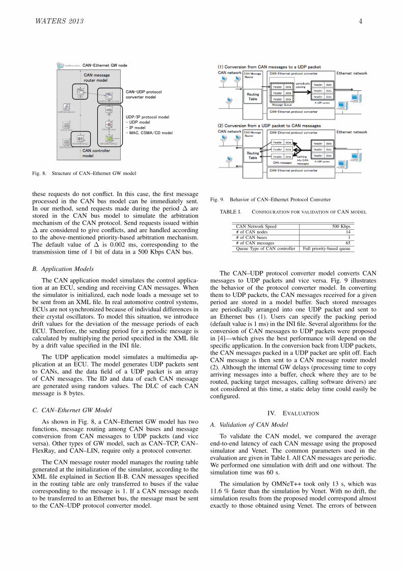
Fig. 8. Structure of CAN–Ethernet GW model

these requests do not conflict. In this case, the first messageprocessed in the CAN bus model can be immediately sent.In our method, send requests made during the period ∆ arestored in the CAN bus model to simulate the arbitrationmechanism of the CAN protocol. Send requests issued within∆ are considered to give conflicts, and are handled accordingto the above-mentioned priority-based arbitration mechanism.The default value of ∆ is 0.002 ms, corresponding to thetransmission time of 1 bit of data in a 500 Kbps CAN bus.

B. Application Models

The CAN application model simulates the control applica-tion at an ECU, sending and receiving CAN messages. Whenthe simulator is initialized, each node loads a message set tobe sent from an XML file. In real automotive control systems,ECUs are not synchronized because of individual differences intheir crystal oscillators. To model this situation, we introducedrift values for the deviation of the message periods of eachECU. Therefore, the sending period for a periodic message iscalculated by multiplying the period specified in the XML fileby a drift value specified in the INI file.

The UDP application model simulates a multimedia ap-plication at an ECU. The model generates UDP packets sentto CANs, and the data field of a UDP packet is an arrayof CAN messages. The ID and data of each CAN messageare generated using random values. The DLC of each CANmessage is 8 bytes.

C. CAN–Ethernet GW Model

As shown in Fig. 8, a CAN–Ethernet GW model has twofunctions, message routing among CAN buses and messageconversion from CAN messages to UDP packets (and viceversa). Other types of GW model, such as CAN–TCP, CAN–FlexRay, and CAN–LIN, require only a protocol converter.

The CAN message router model manages the routing tablegenerated at the initialization of the simulator, according to theXML file explained in Section II-B. CAN messages specifiedin the routing table are only transferred to buses if the valuecorresponding to the message is 1. If a CAN message needsto be transferred to an Ethernet bus, the message must be sentto the CAN–UDP protocol converter model.

!

!

!

!

!

"#$%&'()*+,-'(%.+'/%&01%/*,,23*,%4'%2%567%829:*4!

";$%&'()*+,-'(%.+'/%2%567%829:*4%4'%&01%/*,,23*,!

!"#$"%! $#&#!

!"#$"%! $#&#!

!"#$"%! $#&#!

!"#$"%! $#&#!

!"#$"%! $#&#!

!"#$"%! $#&#!

<*,,23*%=>*>*!

8*+-'?-92@@A!

829:-(3!

&01%(*4B'+:! C4D*+(*4%(*4B'+:!

0%567%829:*4!

&01EC4D*+(*4%8+'4'9'@%9'()*+4*+!

!

!

!

!

!

&01%<*,,23*!

%F'>4*+!

!

!

!

!

!

F'>4-(3!

G2H@*!

&01EC4D*+(*4%8+'4'9'@%9'()*+4*+!

!

!

!

!

!

!"#$"%! $#&#!

!"#$"%! $#&#!

!"#$"%! $#&#!

!"#$"%! $#&#!

!"#$"%! $#&#!

!"#$"%! $#&#!

&01%/*,,23*,!

&01%(*4B'+:! C4D*+(*4%(*4B'+:!

0%567%829:*4!

&01EC4D*+(*4%8+'4'9'@%9'()*+4*+!

!

!

!

!

!

&01%<*,,23*!

%F'>4*+!

!

!

!

!

!

F'>4-(3!

G2H@*!

&01EC4D*+(*4%8+'4'9'@%9'()*+4*+!

,8@-44-(3!

-(4'%&01%

/*,,23*,!

Fig. 9. Behavior of CAN–Ethernet Protocol Converter

TABLE I. CONFIGURATION FOR VALIDATION OF CAN MODEL

CAN Network Speed 500 Kbps# of CAN nodes 14# of CAN buses 1# of CAN messages 65Queue Type of CAN controller Full priority-based queue

The CAN–UDP protocol converter model converts CANmessages to UDP packets and vice versa. Fig. 9 illustratesthe behavior of the protocol converter model. In convertingthem to UDP packets, the CAN messages received for a givenperiod are stored in a model buffer. Such stored messagesare periodically arranged into one UDP packet and sent toan Ethernet bus (1). Users can specify the packing period(default value is 1 ms) in the INI file. Several algorithms for theconversion of CAN messages to UDP packets were proposedin [4]—which gives the best performance will depend on thespecific application. In the conversion back from UDP packets,the CAN messages packed in a UDP packet are split off. EachCAN message is then sent to a CAN message router model(2). Although the internal GW delays (processing time to copyarriving messages into a buffer, check where they are to berouted, packing target messages, calling software drivers) arenot considered at this time, a static delay time could easily beconfigured.

IV. EVALUATION

A. Validation of CAN Model

To validate the CAN model, we compared the averageend-to-end latency of each CAN message using the proposedsimulator and Venet. The common parameters used in theevaluation are given in Table I. All CAN messages are periodic.We performed one simulation with drift and one without. Thesimulation time was 60 s.

The simulation by OMNeT++ took only 13 s, which was11.6 % faster than the simulation by Venet. With no drift, thesimulation results from the proposed model correspond almostexactly to those obtained using Venet. The errors of between

WATERS 2013 4

!"

!#$"

!#%"

!#&"

!#'"

!#("

!#)"

%*'"

%*)"

%+$"

%,!"

%,&"

&$,"

&,*"

'%,"

'&$"

'&)"

',("

)*&"

*+("

*,%"

+,)"

,%+"

,&!"

,&'"

,(%"

,(,"

,**"

,+$"

,+&"

,+("

$!$&"

$%+!"

$(+("

$(++"

$(,$"

$(,("

$(,*"

$(,,"

$)))"

!"#$%&#'#()*+,*#()'-%+#(./'01234

5$6,$6+/',7'8!9':#22%&#4

-./0122" 30405"

Fig. 10. Average end-to-end latency for CAN messages with drift

!"#$ !"%$

&'()*+)'$

,-./#$ ,-./%$ ,-./0$ ,-./1$

Fig. 11. Network configuration for evaluation

30–40 ns are due to rounding errors in the sending time ofCAN messages. Therefore, we consider the CAN model tobe valid in the case of no drift. Fig. 10 shows the results ofthe simulation with drift. The average end-to-end latency errorbetween OMNeT++ and Venet is of the order of a few ms.However, this is greater than the error in the case of no drift.In particular, the error for message ID 1595 is approximately0.2 ms. We can confirm that the rounding error in the sendingtime of CAN messages also caused this error. The number ofdisruptions caused by messages with higher priority differedbetween the two simulators. We consider the above results toagain validate the CAN model.

B. Case Study for a CAN–Ethernet Network

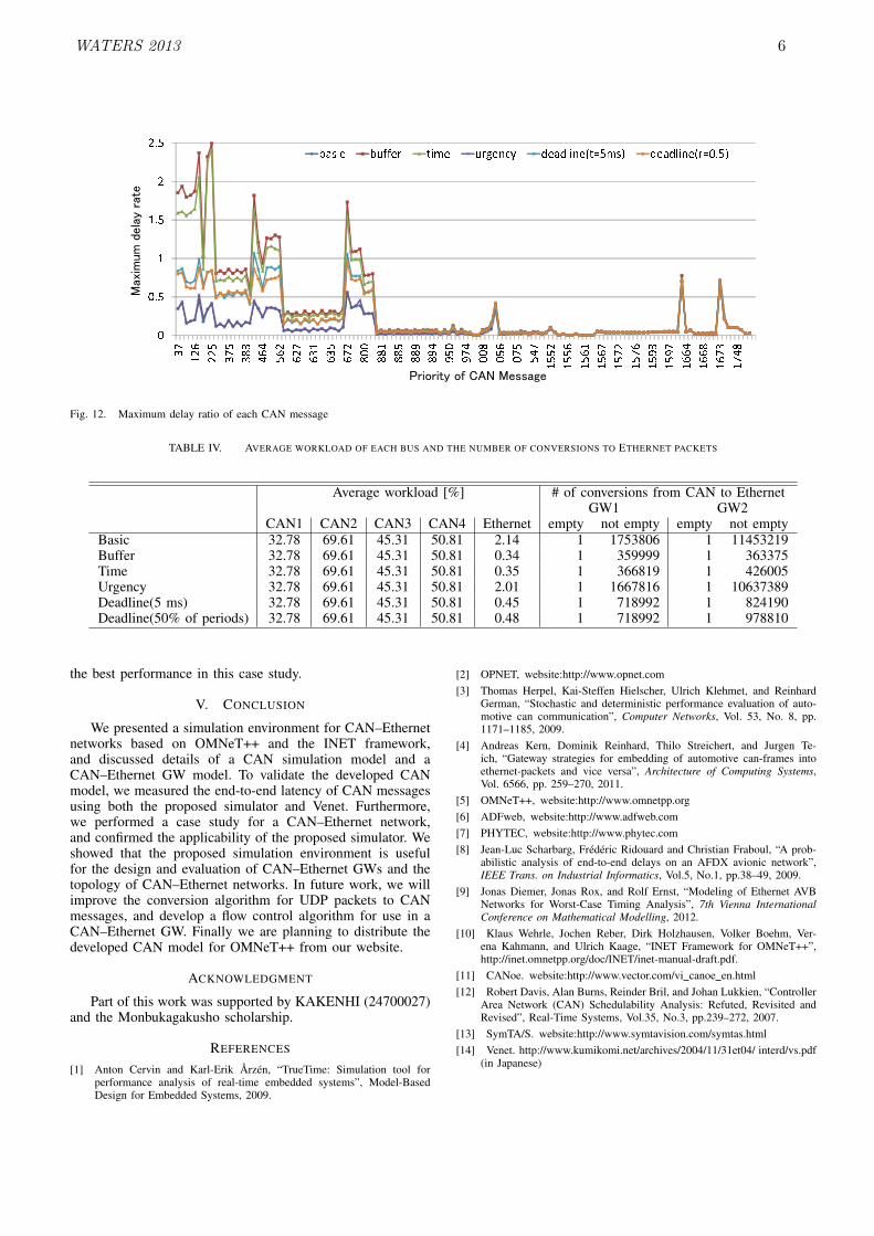
We performed a case study of a CAN–Ethernet network toconfirm the applicability of the proposed simulator. Table IIshows the configuration of the network in this evaluation, andthe network topology is shown in Fig. 11. The network consistsof four CAN buses and an Ethernet bus. These are connectedto CAN–Ethernet GW nodes. The parameters measured inthis evaluation are the maximum end-to-end latency of eachmessage, the maximum latency rate, the buffer usage in eachCAN controller, and the utilization of each CAN bus. Themaximum latency rate is defined as the ratio of the maximumend-to-end latency to the sending period of the message, andis only calculated for periodic messages. If the maximumlatency rate is greater than 1, the message may not arrive at thedestination node prior to the next sending time of the message.

In addition to the algorithms proposed in [4], we proposea heuristic deadline-aware algorithm. For this evaluation, weassumed that the deadline of each message corresponded toits sending period. We assumed two different maximum delaytimes in each CAN network, 5 ms (i.e., a constant value) and

TABLE II. CONFIGURATION OF CAN–ETHERNET NETWORK FORCASE STUDY

CAN Network Speed 500 kbpsEthernet Network Speed 100 Mbps# of CAN nodes 90# of Ethernet buses 1# of CAN–Ethernet GWs 2# of CAN buses 4# of CAN messages 216 (periodic)

194 (aperiodic)Drift of Each Node ± 1%Queue Type of CAN controller Full priority-based queue

TABLE III. PARAMETERS FOR CONVERSION ALGORITHMS

Buffer Conversion Maximum Ratio of Assumedsize period shortened urgent delay time in

[ms] time [ms] messages [%] CAN networkBasic 1 - - - -Buffer 40 20 - - -Time 40 20 20 - -Urgency 40 20 20 20 -

deadline(5 ms) 20 5 - - 5ms

deadline(50% ofperiods)

20 5 - -50% ofperiods

50% of the period of each CAN message. In the deadline-aware algorithm, when a CAN message reaches a GW, itand the messages stored in the GW buffer are packed intothe Ethernet packet if the remaining time to the deadlineof the message is less than 5 ms or 50% of the period ofthe message. In this experiment, the value of the assumeddelay time was heuristically determined, because there is noanalysis method for the worst-case end-to-end delay in CAN–Ethernet networks. Therefore, we found the appropriate valueby changing the parameter in 10% increments, from 10% to90%. The simulation time was 7200 s, which corresponds toone driving cycle.

The maximum delay ratios of each algorithm are shownin Fig. 12. In the case of the deadline-aware algorithm (50%of periods), all messages met their timing constraints. FromFig. 12, we can see that the maximum delay ratio of somemessages is greater than 1 in the basic, buffer, and timealgorithms. This means that the deadline was missed in thesesimulations. For messages with high priorities (i.e., from 1 to300), the conversion period was insufficient to meet the timingconstraints. For messages with lower priorities, the sendingperiod was shorter than for messages with similar priorities.Therefore, the influence of these messages was large.

Table IV presents the average utilization of CAN busesand the number of conversions from CAN to Ethernet. Inthe table, empty refers to the number of conversions to anEthernet packet without any CAN messages, and not emptyrefers to the number of conversions to an Ethernet packetwith CAN messages. The average utilization of each bus issimilar for all algorithms, whereas the difference in averageEthernet utilization is small. The fewest conversions from CANmessages to Ethernet packets for the buffer-type algorithmoccur at GW1. In the deadline-aware algorithm (50% ofperiods), the number of conversions from CAN to Ethernetwas also fewer than for the basic and urgency algorithms.Therefore, the deadline-type algorithm (50% of periods) gave

WATERS 2013 5

!"#$"#%&'$(')*+',-../0-

,/1#232'4-5/&'"/%-

Fig. 12. Maximum delay ratio of each CAN message

TABLE IV. AVERAGE WORKLOAD OF EACH BUS AND THE NUMBER OF CONVERSIONS TO ETHERNET PACKETS

Average workload [%] # of conversions from CAN to EthernetGW1 GW2

CAN1 CAN2 CAN3 CAN4 Ethernet empty not empty empty not emptyBasic 32.78 69.61 45.31 50.81 2.14 1 1753806 1 11453219Buffer 32.78 69.61 45.31 50.81 0.34 1 359999 1 363375Time 32.78 69.61 45.31 50.81 0.35 1 366819 1 426005Urgency 32.78 69.61 45.31 50.81 2.01 1 1667816 1 10637389Deadline(5 ms) 32.78 69.61 45.31 50.81 0.45 1 718992 1 824190Deadline(50% of periods) 32.78 69.61 45.31 50.81 0.48 1 718992 1 978810

the best performance in this case study.

V. CONCLUSION

We presented a simulation environment for CAN–Ethernetnetworks based on OMNeT++ and the INET framework,and discussed details of a CAN simulation model and aCAN–Ethernet GW model. To validate the developed CANmodel, we measured the end-to-end latency of CAN messagesusing both the proposed simulator and Venet. Furthermore,we performed a case study for a CAN–Ethernet network,and confirmed the applicability of the proposed simulator. Weshowed that the proposed simulation environment is usefulfor the design and evaluation of CAN–Ethernet GWs and thetopology of CAN–Ethernet networks. In future work, we willimprove the conversion algorithm for UDP packets to CANmessages, and develop a flow control algorithm for use in aCAN–Ethernet GW. Finally we are planning to distribute thedeveloped CAN model for OMNeT++ from our website.

ACKNOWLEDGMENT

Part of this work was supported by KAKENHI (24700027)and the Monbukagakusho scholarship.

REFERENCES

[1] Anton Cervin and Karl-Erik Arzen, “TrueTime: Simulation tool forperformance analysis of real-time embedded systems”, Model-BasedDesign for Embedded Systems, 2009.

[2] OPNET, website:http://www.opnet.com[3] Thomas Herpel, Kai-Steffen Hielscher, Ulrich Klehmet, and Reinhard

German, “Stochastic and deterministic performance evaluation of auto-motive can communication”, Computer Networks, Vol. 53, No. 8, pp.1171–1185, 2009.

[4] Andreas Kern, Dominik Reinhard, Thilo Streichert, and Jurgen Te-ich, “Gateway strategies for embedding of automotive can-frames intoethernet-packets and vice versa”, Architecture of Computing Systems,Vol. 6566, pp. 259–270, 2011.

[5] OMNeT++, website:http://www.omnetpp.org[6] ADFweb, website:http://www.adfweb.com[7] PHYTEC, website:http://www.phytec.com[8] Jean-Luc Scharbarg, Frederic Ridouard and Christian Fraboul, “A prob-

abilistic analysis of end-to-end delays on an AFDX avionic network”,IEEE Trans. on Industrial Informatics, Vol.5, No.1, pp.38–49, 2009.

[9] Jonas Diemer, Jonas Rox, and Rolf Ernst, “Modeling of Ethernet AVBNetworks for Worst-Case Timing Analysis”, 7th Vienna InternationalConference on Mathematical Modelling, 2012.

[10] Klaus Wehrle, Jochen Reber, Dirk Holzhausen, Volker Boehm, Ver-ena Kahmann, and Ulrich Kaage, “INET Framework for OMNeT++”,http://inet.omnetpp.org/doc/INET/inet-manual-draft.pdf.

[11] CANoe. website:http://www.vector.com/vi canoe en.html[12] Robert Davis, Alan Burns, Reinder Bril, and Johan Lukkien, “Controller

Area Network (CAN) Schedulability Analysis: Refuted, Revisited andRevised”, Real-Time Systems, Vol.35, No.3, pp.239–272, 2007.

[13] SymTA/S. website:http://www.symtavision.com/symtas.html[14] Venet. http://www.kumikomi.net/archives/2004/11/31et04/ interd/vs.pdf

(in Japanese)

WATERS 2013 6

CloudNetSim - Simulation of Real-Time Cloud Computing Applications

Tommaso Cucinotta, Aram SantogidisBell Laboratories, Alcatel-Lucent, Dublin

In this paper, we describe CloudNetSim, a project aim-ing to realise a simulation platform supporting our ongoingand planned research activities in the area of resource man-agement and scheduling for distributed QoS-sensitive andsoft real-time applications. It is based on OMNeT++, in-tegrating in the platform a set of modules for the simula-tion of CPU scheduling, including hierarchical schedulingat both levels of the hypervisor and guest Operating System,as needed when simulating cloud infrastructures. Thanksto the modularity of OMNeT++, CloudNetSim may eas-ily leverage many existing simulation models already avail-able for networking, including standard network compo-nents and protocols, such as TCP/IP. After a brief overviewof related simulation tools found in the literature, and thediscussion of their limitations, we provide a detailed de-scription of the internals of our simulator. Then, we showresults gathered from a few representative scenarios demon-strating how its behaviour matches with the one of simplereal applications.

1 Introduction

Cloud Computing is gaining momentum as one of thekey innovations disrupting the world of computing, consti-tuting a page turn from the old ages of Personal Computingto a new era of massively distributed cloud applications andservices accessed from a plethora of devices with increasedmobility support. Cloud Computing is also generating acontinuous pressure towards the research community, forintroducing innovations and novel mechanisms promisingto support better the nowadays and future computing sce-narios. As connectivity evolves towards higher bandwidthand lower latency, more and more soft real-time (RT) andinteractive on-line applications are becoming increasinglyused and popular [17]. These include many on-line inter-active cloud applications, such as office suites (e.g., GoogleDocs) or e-Learning platforms [7], virtual desktop, and on-line massively parallel games.

When working at the lowest layers of the cloud infras-tructure, and specifically at the hypervisor, Operating Sys-tem (OS), and CPU scheduling levels, it is often difficultif not impossible to gain access to realistic test-beds over

which to carry out research activities in the field. Often,it is very handy and convenient to have available tools thatmay assist researchers in simulating cloud deployments andend-to-end distributed applications, with a sufficient level ofabstraction depending on the research purposes and scope.

However, simulation of distributed soft real-time appli-cations over general-purpose computing platforms and net-works is troublesome due to the lack of proper tools. Vari-ous simulators exist in the areas of networked systems andreal-time systems, and recently a few simulation tools havebecome available in the area of Cloud Computing. In gen-eral, the existing tools were lacking the fundamental abil-ity to integrate the various cross-domain simulation aspectsthat affect the end-to-end performance (see Section 2).

In this paper, we introduce CloudNetSim, a project aim-ing to provide a simulation platform to assist the exper-imentation with resource management and scheduling incloud computing. At a glance, its main features comprise:packet-level simulation of end-to-end network communica-tions between clients and servers distributed throughout acloud infrastructure; simulation of computing resources in-cluding but not limited to CPU scheduling both at the hyper-visor and at the guest OS levels; support for virtual machine(VM) deployment strategies; modularity and extensibility,with the possibility to introduce additional scheduling poli-cies, VM deployment strategies and application models asneeded. We aim to keep an abstraction level that allows forsimulation of thousands of nodes and applications, gather-ing the necessary QoS metrics, within an affordable time.

Even though CloudNetSim targets simulation of cloudapplications, the presented work may also be used for sim-ulating networked soft real-time and embedded systems.

2 Related Work

In this section, the simulation tools mostly related to thepresented work are briefly introduced. They fall roughlyin the categories of real-time systems simulators, networkprotocols simulators and cloud computing simulators.

In the area of RT and embedded systems, many simu-lation tools deal with simulation of CPU scheduling, in-cluding RTSim [18], MAST [10], MAST2 [9], SimTrOS [19]

WATERS 2013 7

and others [1], just to mention a few. However, either theyare exclusively focused on hard RT and embedded systemsand they do not support general-purpose schedulers and re-lated technologies, or they neglect entirely the networkingaspects. Some tools integrate simulation of CPU schedul-ing and technologies/protocols for CAN busses or Wire-less Sensor Networks [6], however these tools are hardlyreusable in the context of general purpose technologies.

In the area of networking and distributed systems, manytools provide an accurate simulation of networking tech-nologies and packet-level simulation of networking proto-cols [21, 11, 20]. For example, NS21 is probably one ofthe most widely known open-source simulators used in re-search about network protocols, whose development startedin 1996. It supports packet-level simulation of many Inter-net protocols and technologies, including TCP/IP and wire-less networks. However, the simulator derives from a quiteold code base, where functionality has been evolving overyears, split around C/C++ and Object Tcl code. This re-sulted in the lack of modularity and clean interfaces for ex-tending its functionality. It is not a case that, from 2004, anew NS32 project was born with the intention of a com-plete redesign of the internals of the simulator, and ulti-mately dropping compatibility with NS2. Unfortunately,this resulted in a set of features not (yet) as complete asin NS2. A completely alternative project is the open-sourceOMNeT++3, free for academic use, and commercially li-censed as OMNEST4. OMNeT++/OMNEST is a simulationplatform with a completely modular design where genericmodules can be connected in arbitrarily complex topolo-gies and communicate with each other, all integrated withan Eclipse-based development environment including a vi-sual topology editor. One of the main uses of OMNeT++ isin connection with the INET Framework5, an open-sourcecommunication networks simulation package including aset of modules for simulation of Internet technologies andprotocols, including TCP/IP, IPv6, Ethernet, PPP, 802.11,MPLS, and others.

However, all of these network simulators simply do notinclude any CPU scheduling infrastructure. In a cloud en-vironment, where multiple VMs may be multiplexed on thesame physical host, processor and core, it is important tosimulate CPU scheduling, to get a comprehensive pictureof the end-to-end response-time and performance. Espe-cially when dealing with low-latency cloud applications de-ployed in future scenarios with fine-grained cloud data cen-tres, tools are needed to support a comprehensive and inte-grated simulation of multiple resources, such as CPU, net-

1More information at: http://www.isi.edu/nsnam/ns/.2More information is available at: http://www.nsnam.org/.3More information is available at: http://omnetpp.org/.4More information is available at: http://www.omnest.com.5More information at: http://inet.omnetpp.org/index.php.

work and storage, that allow for modelling distributed ap-plications, particularly those with QoS requirements, devel-oped in the context of general-purpose technologies.

Recently, a few simulation tools have become avail-able [2, 14, 4, 12] targeting the specific simulation needsarising in the area of Cloud Computing. CloudSim [2] isa Java-based simulation platform modelling various aspectsof cloud computing infrastructures such as high-level sim-ulation of data centres with virtualized hosts, energy con-sumption models and federated clouds. Versions prior to 2.0have a very simple networking model at the flow level, withstatically configured latency and bandwidth values amonglocations, while from version 2.0 a better network simula-tion functionality was added.

CloudSim is derived from GridSim [3], thus its architec-ture is still strongly tied to the modelling and simulation ofGRID scenarios, with a focus on load balancing within thedata centre, rather than gathering performance metrics overend-to-end deployments of general-purpose cloud comput-ing applications, as in our proposed CloudNetSim.

iCanCloud [14, 4] is a simulator platform for cloud com-puting based on OMNeT++, with the capability to configurevarious resource management policies for the hypervisor,virtual machine models aiming to simulate the behaviour ofreal world CPUs, data centre topologies that mimic the ar-chitecture of state of the art cloud computing infrastructures(e.g. Amazon EC26) and data storage emulation. Still, thistool is lacking the essential capability to simulate the varietyof heterogeneous networks involved in the end-to-end cloudservice supply chain. However, being based on OMNeT++as our framework, iCanCloud has interesting modules thatwe might re-use, such as the storage models inherited fromSIMCAN [16, 15], a simulator of local and remote storagesystems, including NFS and parallel file systems.

GreenCloud [12] is an NS2-based C++ simulator aimingto model the energy consumption of data center IT equip-ment (e.g. computers, network switches and communica-tion links), to help the design of energy efficient architec-tures. However, GreenCloud needs merely a rough estimateof the expected computing workload on the nodes, for itspower consumption estimates.

Overall, some of the mentioned simulators targetingcloud computing focus specifically on aspects of the in-frastructure related to computing within the data centre, ne-glecting the important aspects of communications over theInternet or the access network. Others try to enrich an accu-rate simulation of the network by adding rough computingmodels which cannot capture a similar level of detail, whenaddressing QoS and responsiveness. However, considera-tion of the whole end-to-end chain is very important for theoverall QoS delivered to remote customers/users.

As a consequence, we could not find in existing tools

6More information is available at: aws.amazon.com/ec2/.

WATERS 2013 8

OMNEST

INET

Client Cloud

Data center

Figure 1. High-level software architecture

features properly matching with the particular needs of re-search on the topics of resource management and schedul-ing for interactive, real-time and low-latency cloud and dis-tributed applications.

3 Proposed Approach

One of the primary goals of the overall ongoing Cloud-NetSim project is to integrate within a single simulationplatform the major factors contributing to end-to-end la-tency of low-latency cloud applications, namely network-ing, computing and disk access, including overheads due tovirtualization (both machine and network virtualization).

We opted to implement the computing part of the simu-lation on top of OMNEST (see Figure 1), due to its relativematurity, modular design and extensibility. We realized aset of OMNEST modules in order to model computing andCPU scheduling within physical hosts and VMs, as happen-ing within a cloud computing data centre; these inter-mixwith the already available network communication mod-ules, resulting in a more comprehensive emulation of themajor contributions to end-to-end response-times. At thispreliminary stage, disk access has been greatly simplified,but we plan to consider it more thoughtfully later.

Simulating large infrastructures with such a fine-grainedlevel of detail for computing and networking resources maypresent performance and scalability challenges. However, ithas been shown [13] that parallelisation techniques can beeffectively applied to OMNeT++ simulations in a seamlessfashion, without requiring changes in the code. These willcertainly be useful for our planned future investigations.

Overall Design. The core component for modelling com-puting elements is CloudNode. It is built on top of the Node-Base compound module of INET which models a networkhost, and provides interface and network layer functionality.CloudNode additionally incorporates a number of modulesthat emulate the computing part of the module (see Fig-ure 2), i.e., the CPU Scheduler, modules for applicationsand for data storage emulation. Moreover, the CloudNode

Figure 2. OMNEST representation of a simpletopology.

modules can be interconnected with each other in a hierar-chical fashion, effectively modelling VMs running within aphysical host. Figure 2 illustrates the topology of a clientconnected through a router to a host running 3 VMs.

In OMNEST terminology, CloudNode is a compoundmodule that extends NodeBase (see Figure 3 for anoverview of its inner design). It is an aggregation of sim-ple modules that allow for modelling various aspects of thesoftware stack typical of virtualized infrastructures. As de-picted in Figure 3, CloudNode includes simulation of net-work capabilities as inherited from NodeBase, data stor-age and CPU scheduling. The networking capabilities havebeen customised by adding SchedPPP, a module extendingthe INET PPP interface which is controllable from the CPUscheduler. This is necessary in order to “suspend” the net-work connectivity of a VM, when it is preempted from ex-ecution by the CPU scheduler. A similar SchedEth modulehas been realised for Ethernet.

The Scheduler within a CloudNode is able to schedule anarbitrary number of Schedulable entities over a configurablenumber of available CPUs. Also, these can be connected toa data storage model in order to model suspension on I/O.Interestingly, a CloudNode is schedulable on its own. Thisallows VMs to be modelled as CloudNode instances con-nected to the Scheduler of the outer CloudNode represent-ing the host they are deployed within.

Scheduler Design. Schedulable entities represent soft-ware running in the system, including both applications orcomponents at the hypervisor level, and those within guestVMs. The Schedulable interface permits the Scheduler to

WATERS 2013 9

Network

Layer

Transport

Layer

Wlan PPP Eth SchedPPP

NodeBase

radioIn ethgpppg spppg

Schedulable Entity

CPU Core

Scheduler

Storage

Medium

Data I/O

scheduleOut

CloudNode

Network I/O

Figure 3. CloudNode design.

Figure 4. Schedulable entities FSM.

manage their execution state. All these entities extend theBaseSchedulable class that implements the well-known Fi-nite State Machine (FSM) in Figure 4. The logical com-munications between the Scheduler and its managed en-tities, necessary to realise the mentioned FSM behaviour,is conducted through the scheduleIn/scheduleOut ports ofthe Schedulable interface, by exchanging custom definedOMNEST messages. Specifically, the Scheduler notifiesready-to-run entities whenever a CPU is assigned or re-voked to them, according to the scheduling algorithm in usewithin the Scheduler. The entities, on their own, notify theScheduler whenever they need to suspend for data I/O, net-working, or timer operations.

The CPU is modelled in the scheduler with a few config-urable parameters controlling its power-saving capabilities,including the frequency at which it is running, and whetherit is in a deep-idle state. Therefore, messages from theScheduler to the entities also include the frequency change

information, needed to allow applications to modulate theirexecution time behaviours accordingly. This allows for sim-ulation of multi-processor and multi-core hosts with CPUpower-saving capabilities. However, an exact strategy toswitch among the available CPU frequencies (i.e., mimick-ing the behaviour of the cpufreq governors in Linux) isstill work in progress. Also, we only modelled a single idle-state of the CPU with a configurable wake-up latency, as atthe moment there is no interest in modelling the multitudeof idle states in modern CPUs.

We realised 3 scheduling algorithms: Fixed Prior-ity (FP), Round-Robin, Linux Completely Fair Scheduler(CFS). These can be hierarchically composed with eachother. This is shown through the example in Figure 5.(a),where a typical Linux set-up is shown with 6 applica-tions running under various scheduling policies, as detailedin Figure 5.(b). With the proposed architecture, multi-ple real-time tasks at the same priority under the POSIXSCHED RR policy are represented as connected to an in-stance of the Round-Robin Scheduler, which in turn is con-nected to the FP Scheduler at the needed priority level.Also, SCHED OTHER tasks are connected to a CFS Sched-uler connected to the FP Scheduler at priority 0.

Configuration of the Scheduler(s) topology is simpli-fied by specifying for each application the desired schedul-ing parameters (including the nice level, in case ofSCHED OTHER entities), and the CloudNode instantiatesthe required Scheduler modules and interconnections asneeded. Note that the overall Scheduler design allows foran easy introduction of new algorithms.

Application Model. Applications are modelled in Cloud-NetSim as Schedulable entities, executing sequentially a listof instructions. Following the steps of RTSim [18], thepurpose of the simulation is not functional simulation, butrather performance evaluation. Therefore, allowed instruc-tions are for now: computing for a fixed amount of time(scaled linearly with the CPU frequency); wait for the trans-fer of a fixed number of blocks to/from the storage medium;change dynamically the scheduling parameters of the appli-cation. Also, a few instructions are being realised allowingfor modelling (the impact on performance of) communica-tions among various parts of a distributed cloud application.

A convenience scripting syntax has been defined, so thatsimple application models may easily be provided throughtext-based input files to the simulation.

4 Calibration and Simulation Experiments

In this section we report results from a few experimentswe ran in order to show how the parameters of the simulatedmodels may be calibrated so that its outcome matches withthe behaviour measured from a real simple scenario.

WATERS 2013 10

CPU

FIFO Scheduler

App 0

App 1 App 2App 3

App 4App 5

rt-prio=3

rt-prio=10

CFS Scheduler

Round-Robin

Scheduler

rt-prio=0

nice=0 rt-prio=0

nice=0

rt-prio=0

nice=0

SCHED_FIFO[0]

SCHED_FIFO[10]

rt-prio=10

(a)App Priority Policy

0 3 SCHED FIFO1 10 SCHED RR2 10 SCHED RR3 0 SCHED OTHER4 0 SCHED OTHER5 0 SCHED OTHER

(b)

Figure 5. Hierarchical scheduling of pro-cesses based on policy

Real world SimulationHost (idle) 0.384 +/- 0.040 ms 0.388 msHost (hog) 0.322 +/- 0.034 ms 0.333 msVM1 (idle) 0.482 +/- 0.034 ms 0.462 msVM1 (hog) 0.377 ms +/- 0.036 ms 0.399 ms

Table 1. Ping times statistics for the real-world(left) and simulated (right) scenarios.

Ping Test. We consider a simple topology with a physicalhost running two VMs connected through a network routerto a client that pings the physical host and the VMs (seeFigure 2). After calibration of the simulation model pa-rameters, its results are compared with numbers obtainedby the corresponding real-world example. In the latter,we used an Intel i5-2520M @ 2.50GHz laptop client ping-ing a Linux machine equipped with an Intel Xeon E5-2687W CPU whose frequency was fixed at 3.1 GHz, and inwhich all cores except one have been put offline, and hyper-threading has been disabled, to create the simple scenarioreproduced in simulation. Also, a guest KVM Linux OShas been run on the server machine. The host and the VMhave been continuously pinged for one minute every halfsecond, when the host was idle, and when it was loaded.The obtained ping times average and standard deviation areshown in Table 1, in both real-world and simulated cases.

The overall ping latency towards the host is the resultof summing up delay contributions due to network delay toreach the server, CPU wake-up from idle,networking stack

execution for replying to the ping, then back to the client.When pinging the VM, further contributions are due to thecontext switch to schedule the VM and guest OS network-ing stack execution for replying to the ping.

CFS Test. We ran another ping experiment using the CFSas the hypervisor scheduler. We verified that, despite a 2ndVM hogging the CPU, the pinged idle VM was respondingimmediately to the ping, preempting the other one. This be-haviour is in sync with the CFS algorithm since the pingedVM, waking up from a blocked state, runs immediately,since its virtual run-time is much lower than the one of theCPU-bound VM continuously executing.

Then, to verify the behaviour of the CFS in presence ofdifferent nice values, we considered another simple scenariowith three applications running CPU bound tasks on a hostand we compared the obtained simulated versus real figures.

We use a load.sh shell script realising a simple forloop for the number of iterations provided as argument.When running on an Intel i5-2520M CPU at fixed 2.50 GHzfrequency, load.sh takes 1 second to complete with anargument of 177000. In single-core mode, we run threetasks with the default nice value (0), however the third oneis reniced to (10) at half execution. This is obtained as:

time ./load.sh 177000 &time ./load.sh 177000 &time ./load.sh 88500time nice ./load.sh 88500

The obtained results show that the first two processescompleted in less than 2.6 seconds, whilst the reniced pro-cess completed after 1.56 + 1.49 = 3.05 seconds:

0.47u 0.02s 1.56r ./load.sh 885000.93u 0.03s 2.55r ./load.sh 1770000.95u 0.03s 2.58r ./load.sh 1770000.51u 0.00s 1.49r nice ./load.sh 88500

The same experiment has been arranged in the simulatedmodel, using the renice instruction explained in the previ-ous section for changing dynamically the third process nicelevel at half of its execution. This resulted in the followingoutput, gathered from the OMNeT++ logs:

T=3.004008 TestCloudNode.srv.tcpApp[0]T=2.560008 TestCloudNode.srv.tcpApp[1]T=2.554008 TestCloudNode.srv.tcpApp[2]

These results validate the correct behaviour of the CFSScheduler model, in the mentioned scenario.

5 Conclusions and Future Work

In this paper we presented CloudNetSim, a simulationplatform suitable for capturing the behaviour of end-to-end

WATERS 2013 11

time-sensitive and particularly low-latency distributed ap-plications. The platform exploits the native OMNEST andINET capabilities for network simulation, integrating simu-lation of computing and storage access in virtualized envi-ronments. We plan to use this platform for our ongoing andplanned research in the area of resource management andscheduling for soft real-time cloud computing applications.The presented simulation models are very important to sim-ulate the impact on performance of sharing physical com-puting resources within the infrastructure, as often done bycloud providers trying to achieve high consolidation levels.However, CloudNetSim may also be useful for simulationof soft real-time distributed embedded systems.

The presented work may be extended along various linesof action: the CPU scheduling models may be refined byadding further scheduling policies, e.g., one mimicking theXen scheduler [5, 8]; the storage access model is very sim-ple, but re-usable modules from other projects such as SIM-CAN might be integrated; the performance achievable withthe integrated multi-resource simulation on large scale sys-tems has to be checked, an area where parallelisation tech-niques such as [13] might be useful.

References

[1] M. Ashjaei, M. Behnam, and T. Nolte. The design and im-plementation of a simulator for switched ethernet networks.In Proc. of the 3rd International Workshop on Analysis Toolsand Methodologies for Embedded and Real-time Systems,pages 57–62, Pisa, Italy, July 2012.

[2] R. Calheiros et al. Cloudsim: a toolkit for modeling andsimulation of cloud computing environments and evaluationof resource provisioning algorithms. Software: Practice andExperience, 41(1):23–50, 2011.

[3] R. N. Calheiros, R. Ranjan, C. A. F. D. Rose, and R. Buyya.Cloudsim: A novel framework for modeling and simula-tion of cloud computing infrastructures and services. CoRR,abs/0903.2525, 2009.

[4] G. Castane, A. Nunez, and J. Carretero. iCanCloud: A briefarchitecture overview. In Parallel and Distributed Process-ing with Applications (ISPA), 2012 IEEE 10th InternationalSymposium on, pages 853–854, 2012.

[5] L. Cherkasova, D. Gupta, and A. Vahdat. Comparison of thethree cpu schedulers in xen. SIGMETRICS Perform. Eval.Rev., 35(2):42–51, Sept. 2007.

[6] M. Chitnis et al. Impact Of The Operating System on theQoS offered by an IEEE 802.15.4-compliant Sensor Net-work. In Proceedings of the 7th IFAC International Con-ference on Fieldbuses and networks in industrial and em-bedded systems, Tolouse, France, Nov 2007.

[7] T. Cucinotta et al. Virtualised e-learning with real-time guar-antees on the irmos platform. In Proceedings of the IEEE In-ternational Conference on Service-Oriented Computing andApplications (SOCA 2010), pages 1–8, Perth, Australia, De-cember 2010.

[8] G. Dunlap. Scheduler development update. Xen SummitAsia 2009, Shanghai, 11 2009.

[9] M. G. Harbour et al. Modeling real-time networks withmast2. In Proc. of the 2nd International Workshop on Anal-ysis Tools and Methodologies for Embedded and Real-timeSystems, pages 51–56, Porto, Portugal, July 2011.

[10] M. G. Harbour, J. J. G. Garcıa, J. C. P. Gutierrez, andJ. M. D. Moyano. Mast: Modeling and analysis suite forreal time applications. In Proceedings of the 13th EuromicroConference on Real-Time Systems, ECRTS ’01, pages 125–,Washington, DC, USA, 2001. IEEE Computer Society.

[11] T. Issariyakul and E. Hossain. Introduction to Network Sim-ulator NS2. Springer, 2009.

[12] D. Kliazovich, P. Bouvry, and S. U. Khan. A packet-levelsimulator of energy- aware cloud computing data centers.Journal of Supercomputing, 62(3):1263–1283, 2012.

[13] D. Lugones, K. Katrinis, M. Collier, and G. Theodoropou-los. Parallel simulation models for the evaluation of fu-ture large-scale datacenter networks. In Proc. of the 2012IEEE/ACM 16th International Symposium on DistributedSimulation and Real Time Applications, DS-RT ’12, pages85–92, Washington, DC, USA, 2012.

[14] A. Nunez, J. L. Vazquez-Poletti, A. C. Caminero, G. G.Castane, J. Carretero, and I. M. Llorente. iCanCloud: Aflexible and scalable cloud infrastructure simulator. J. GridComput., 10(1):185–209, Mar. 2012.

[15] A. Nunez et al. Design of a flexible and scalable hyper-visor module for simulating cloud computing environments.In Performance Evaluation of Computer TelecommunicationSystems, International Symp. on, pages 265–270, 2011.

[16] A. Nunez, J. Fernandez, J. Garcia, and J. Carretero. Newtechniques for simulating high performance MPI applica-tions on large storage networks. In Cluster Computing, 2008IEEE International Conference on, pages 444–452, 2008.

[17] E. Oliveros, A. Mazzetti, W. Huther, and A. Menychtas. Ir-mos deliverable d2.1.3 - final version of requirements analy-sis report. Technical report, IRMOS Consortium, Nov 2010.

[18] L. Palopoli, G. Lipari, G. Lamastra, L. Abeni, G. Bolognini,and P. Ancilotti. An object-oriented tool for simulatingdistributed real-time control systems. Softw. Pract. Exper.,32(9):907–932, July 2002.

[19] J. Schneider, M. Bohn, and C. Eltges. SimTrOS: A Het-erogenous Abstraction Level Simulator for Multicore Syn-chronization in Real-Time Systems. In Proc. of the 2nd In-ternational Workshop on Analysis Tools and Methodologiesfor Embedded and Real-time Systems, pages 39–44, Porto,Portugal, July 2011.

[20] A. Varga and R. Hornig. An overview of the omnet++ sim-ulation environment. In Proceedings of the 1st internationalconference on Simulation tools and techniques for communi-cations, networks and systems & workshops, Simutools ’08,pages 60:1–60:10, Brussels, Belgium, 2008. ICST.

[21] E. Weingartner, H. vom Lehn, and K. Wehrle. A perfor-mance comparison of recent network simulators. In Pro-ceedings of the IEEE International Conference on Commu-nications 2009 (ICC 2009), Dresden, Germany, 2009. IEEE.

WATERS 2013 12

A Simulation Tool for Optimal Phasing of Nodes

Distributed over Industrial Real-Time Networks

Sang-Hun Lee Hyun-Wook Jin

Dept. of Computer Science and Engineering

Konkuk University

Seoul, Korea

{mir1004, jinh}@konkuk.ac.kr

Kanghee Kim

School of Electronic Engineering

Soongsil University

Seoul, Korea

khkim@ssu.ac.kr

Abstract—Emerging industrial real-time networks, such as

EtherCAT and PROFINET, provide highly accurate clock

synchronization. Thus, this feature opens a new chance to adjust

phasing across distributed nodes aiming for better

synchronization of dependent tasks. However, obtaining an

optimal node phasing across distributed nodes has not been given

enough attention while the worst-case task phasing on each node

assuming no global clock has been studied in many ways. In this

paper, we suggest a simulation tool that searches for an optimal

phasing on distributed nodes with respect to less end-to-end

delays and less actuation jitters. The proposed tool holistically

simulates task scheduling on each node, transmission of network

messages, DMA, and I/O event handling. It tries to reduce the

time to find an optimal node phasing by skipping uninteresting

phase combinations. Through a case study, we show that the

simulator can efficiently suggest an optimal node phasing across

distributed nodes and provide distribution of possible end-to-end

delays and actuation jitters for given task sets.

Keywords—node phasing; industrial network; end-to-end delay;

actuation jitter; clock synchronization

I. INTRODUCTION

Emerging industrial real-time networks, such as EtherCAT [1] and PROFINET [2], provide highly accurate clock synchronization between distributed nodes. For instance, the distributed clock of EtherCAT can provide accurate clock synchronization with errors less than few tens of nanoseconds [3][4]. PROFINET uses Precision Transparent Clock Protocol (PTCP) for clock synchronization. Such accurate clock synchronization opens a new chance to adjust phasing across distributed nodes aiming for better synchronization of dependent tasks (e.g., multi-axis motion controls).

However, obtaining an optimal phasing across distributed nodes has not been given enough attention while the worst-case task phasing on each node has been studied in many ways [5][6]. This is mainly because there has been limited support for clock synchronization on legacy industrial networks and thus researchers have focused on analysis of the worst-case end-to-end delays between tasks assuming no global clock. In order to find the worst-case end-to-end delays, existing studies suggest an analytical model based on a worst-case task phasing

on every node, but they introduce too much pessimism into the analysis [7][8]. However, once we make an assumption of a precise global clock for all the nodes, we can investigate into the problem of finding a phase combination in order to reduce the end-to-end delays and the actuation jitters. The problem can be dealt with by a simulation approach or an analytical approach.

In this paper, we propose a simulation framework that searches for an optimal node phasing on distributed nodes with respect to the end-to-end delays and the actuation jitters. The proposed framework considers behavior of several components composing the target system in a holistic manner to analyze the impact of node phasing on the metrics. The target system is assumed to interconnect one master and multiple slave nodes with a real-time network such as EtherCAT. In our framework, we model each node as a set of periodic tasks scheduled by a fixed-priority scheduling algorithm. In addition, we consider interactions between the nodes and the network, which include network event handling in either polling or interrupt mode, message queuing on network device, and direct memory access (DMA). In the simulation, we also take into account the communication delays in the real-time network, which are affected by the packet forwarding scheme at each node and the network topology.

One novelty of the proposed framework is that we try to reduce the time to find an optimal node phasing by skipping uninteresting phase combinations. Usually, an exhaustive search needs to consider a huge number of phase combinations, which is not tractable. We search for a limited set of the node phase combinations based on the observation that only a few specific states produce an unpredictable trend of end-to-end delays and actuation jitters. That is, our framework runs simulation only for phase combinations that generate such interesting states, while the target metric for other predictable states are calculated by using simple mathematical equations. Through a case study, we show that the proposed simulation framework can efficiently suggest an optimal node phasing across distributed nodes and provide distributions of the end-to-end delays and the actuation jitters for given task sets.

The rest of the paper is organized as follows. Section II describes the system model we assume. In Section III, we suggest our simulation framework for optimal node phasing. Section IV shows a case of finding an optimal node phasing for

This work was supported by the National Research Foundation of Korea (NRF) grant funded by the Korea government (#2012R1A2A2A02015266

and # 2011-0020905).

WATERS 2013 13

a given task set, and Section V summarizes the related work. Finally, in Section VI, we conclude the paper.

II. SYSTEM MODEL

We consider a distributed real-time system that interconnects one master node and N slave nodes with a real-time fieldbus such as EtherCAT, which is common in many industrial applications. For example, a motion control system has such a system configuration where the master node generates position commands to describe the motion trajectory and the slave nodes are motor drives to respond to the commands. In the following, we explain the node model and the network model.

A. Node Model

We consider a set of periodic tasks for both the master and the slave nodes. All the slave nodes are assumed to have the same set of tasks for the sake of brevity, which is not necessary for our simulation framework. The master node may have a different set of tasks than that of the slave nodes. The tasks are denoted by for node m, where n can be different

for the master (m = 0) and the slaves ( ). We denote

each task by

, where and

are its minimum and maximum execution time,

respectively, and is its period. Each task gives a rise of an

infinite sequence of jobs.

denotes the job of . The

release time of

is denoted by

, and the release time of

the first job, i.e., , is called the phase of and denoted by

( < ) In our simulation framework, we

assume the critical instant (i.e., 2 m ⋯ n m ) in each node with a single-processor. In the paper, we focus on finding an optimal combination of the node phases, which are represented by 2 in Fig. 1. The node phase can be varied between 0 and

. ( is the least common

multiple of the periods of all tasks in node m.) We assume that the deadline of each job is the same with the end of its period.

For the scheduling algorithm, we assume a fixed-priority scheduling algorithm such as Rate Monotonic [9]. Since each task is assigned a static priority, the execution of a lower priority task can be preempted by a higher priority task. Thus,

the response time of

reflects the delay due to such

preemption and is denoted by

.

In our task model, to address a realistic scenario commonly found in many industrial networks, we assume that only one task can access the network device for each node. The rationale behind this is that many industrial network protocols do not support multiplexing and de-multiplexing between tasks [10][11]. Moreover, as the name implies, only the master node is assumed to initiate a message transmission. Each slave node may only piggyback some data with the sender task on the message passing through the node on the fly, but cannot initiate a message transmission. Once the sender task at the master creates a message and passes it to the network device, the message experiences a queuing delay in the device, denoted by in Fig. 1, and then is transmitted through the network.

Likewise, when the message arrives at a slave node, it requires

a message handling time, denoted by , before it becomes available to the receiver task.

Fig. 1. System model

B. Network Model

We assume a real-time fieldbus, such as EtherCAT, for real-time communications between the nodes. EtherCAT guarantees deterministic communication delays between any two nodes by the following two design choices. The first one is that it interconnects any two adjacent nodes with a dedicated link in a daisy-chain manner. That is, there are no interfering nodes between nodes m and m+1, and thus no packet collisions on the link. The second one is that each slave node m conducts wormhole switching to relay the packets between nodes m-1 and to m+1, not store-and-forward switching. This switching scheme implemented at the hardware level eliminates the chances that internal software operations of each slave contribute to the end-to-end communication delay. As a result, EtherCAT guarantees deterministic communication delays from the master to any slave m, which is analyzed by Pritz et al. [12] as follows:

𝑠 + − × + 𝑟 𝑠 , (1)

where is the communication delay from the master’s memory to slave m’s memory. 𝑠 is the total transmission time of a message of size s on the master network device. is the total forwarding time of a message on the

slave side, which is a constant of 1 𝜇𝑠 , irrespective of the message size. 𝑟 𝑠 is the total reception time of a message of size s on the slave network controller.

In our simulation framework, we adopt the above delay model expressed by Eq. 1. Therefore, the end-to-end delay from the release time of an initiator task at the master to the completion time of an actuator task at slave m can be described as follows:

2 𝑟 + + , (2)

WATERS 2013 14

where 𝑟 is the delay between the release time of the initiator task at the master and the completion time of the sender task plus the queuing time , and is the

delay between the arrival time of a message at slave m and the completion time of the actuator task. It is important to understand that, in Equation 2, only may be affected by the node phase thus by changing the value of , we may be able to minimize the end-to-end delays and the actuation jitters.

In our simulation framework, the target metrics we want to analyze are the end-to-end delays, the actuation jitters, and the minimum possible queue size q at the network interface that does not cause any packet to be dropped for the entire simulation time, that is, . In the next section, we will describe the proposed simulation framework that gives the target metrics by finding an optimal combination of the node phases 2 .

III. THE PROPOSED FRAMEWORK

In this section, we describe the proposed simulation framework that finds an optimal phasing for distributed nodes. The framework is based on discrete-event simulation to simulate task scheduling, message transmission/forwarding, DMA, and I/O event handling.

A. Overall Design

The simulator is based on the system model described in Section II. Fig. 2 shows the overall design of the proposed simulator. It consists of four components: input file parser, simulation kernel, node objects, and log manager. Configuration parameters, such as number of nodes, task sets, network bandwidth, message size, and event handling mode, etc., are defined in the configuration file in XML format. The file parser reads this configuration file at the initialization phase and passes them as environment variables to the simulation kernel. Then the kernel actually performs simulation loops changing node phasing. The node objects store the run-time snapshot of each node. The log manager stores every event generated during simulation to output files so that user can replay the simulation manually.

B. Node Objects

As mentioned above, the node objects hold a snapshot of run-time image of each node, such as state information of run queue, message queue, and network controller.

The run queue stores task control blocks, each of which has

,

, , mission, and the amount of time that the

corresponding task executed, called etime in this paper. The mission is classified into four categories in the current implementation: send, receive, actuation, and other. This information decides the behavior of the task. More details of this information are described in the next subsection. The

etime variable represents time units consumed by the task in the current period.

The message queue stores network messages, which are yet to be sent to the network or yet to be consumed by a receive task. The queue traces its length at time t and reports the maximum queue length at the end of simulation.

The network controller decides the message transmission speed based on the bandwidth information. It maintains the remaining bytes of a message being sent.

Fig. 2. Overall design of simulator

C. Simulaton Kernel

The simulation kernel comprises clock emulator, CPU emulator, and network emulator. The clock emulator simulates synchronized global clock (e.g., distributed clock of EtherCAT) and increases its counter for every simulation loop.

The CPU emulator runs task(s) on each node for every time unit. The scheduler selects a task to run, and the task executer emulates the behavior of the selected task based on its mission information as mentioned in the previous subsection. If the mission is send, the task executer posts a send request to the network device at the end of execution time of the job. On the other hand, in the receive case, the task executer consumes a message from the message queue at the starting point of the job. When the mission is actuation, the task executer reports that an actuation has taken place at the completion time of the task.

The task executer simply increases the etime value for tasks of other mission. Our current implementation only supports RM scheduling algorithm but our design is general enough to add other scheduling algorithms.

The network emulator simulates operations of the network device (e.g., message transmission, DMA, and raising an interrupt). Event handling can be done in either polling or interrupt mode. If the network device is configured as a polling-based device, the event is handled when a receive task is released. Thus, in this case, the network emulator silently inserts a received message into the receive queue without any notification. When the network device is configured as an interrupt-based device, the network emulator sends an interrupt signal to the CPU emulator so that the interrupt handler is invoked as soon as a message arrives preempting a running task.

To get results for a given phase case, the kernel runs simulation loops emulating operations described above on each node for every time unit.

D. Optimizing Search Time

If the simulator exhaustively repeats the steps described in the previous subsection for all possible combinations of phases, the search time for an optimal node phasing would be very

FileParser

Configure File

LogManager

Log File

TXT

GlobalClock

Sch

edule

r

Task

Exe

cute

r

CPU Emulator

Eve

nt

Handle

r

Counter

Node n

Node 0

TaskRun

Queue

MessageQueue

Simulation Kernel

Node O

bje

cts

TaskRun

Queue

MessageQueue

Network Emulator

Network Device

Clock Emulator

WATERS 2013 15

significant. This search time increases linearly or even exponentially as number of nodes or possible phasing range becomes larger. These also affect the volume of disk I/O performed by the log manager, which is one of dominant overheads of the simulator.

Fig. 3. Possible correlation states

Fig. 4. End-to-end delay variation by changing phase

In order to tackle this issue, we try to reduce the number of phases we investigate while we still gather information for all possible phases. It is important to understand the correlation between phase and end-to-end delay to find interesting phase points. We can easily notice that the phase of a slave node does not affect other slaves’ end-to-end delay by the system model described in Section II. This means that we do not need to consider all combinations of node phases for simulation but can concentrate on phases for each node independently. Due to this characteristic, we can reduce the number of simulation loops.

During simulations, we also observed that in most cases the end-to-end delay increased as phase became larger. Moreover, we found that at some points the end-to-end delay started showing a constant value for a while or reduced suddenly to a very small value as phase became larger. By analyzing these results further, we noticed that a phase resulted in one of states shown in Fig. 3, and the trend of end-to-end delay was changed when a state is changed from one to another by a new phase. Thus, by simulating only for phase points that changes the state, we can significantly reduce the number of simulation loops.

Fig. 4 shows an example of end-to-end delay variation as the discrepancy between phases of the master and a slave increases. Numbers in the figure present state transitions. As we can see in the figure, the end-to-end delay increases in most cases, while the slope of the line is changed (when the state

changes from S1 to S4 and from S2 to S1) or the line is disconnected (when the state changes from S4 to S3).

IV. SIMULATION EXAMPLE

In this section, we run a case to show that the proposed simulation framework can efficiently suggest an optimal phasing across distributed nodes and provide distributions of the end-to-end delays and the actuation jitters for given task sets.

A. Configuration

Table I shows the task set we run on slave nodes. We refer the task set defined in Kim et al. [13] for a motor drive. Each slave node schedules these tasks using the RM algorithm. Table II shows the configuration parameters. We borrow network parameter values, such as queue size, bandwidth, and forwarding delay, from EtherCAT.

TABLE I. TASK SET OF SLAVE NODE

Task Name Period

(us) Execution Time (us)

Description

MotorAct 250 25~35 Controls a motor, and is assigned the highest priority

RtMsg 250 10~15

Receives real-time messages from the network, and shares it with the MotorAct task

NrtMsg 250 7~10

Handles non-real-time messages, and is assigned a lower priority than the RtMsg task

HealthMon 500 6~9

Performs health monitoring, and is assigned the lowest priority

TABLE II. CONFIGURATION PARAMETERS

Parameters Value

Number of slave nodes 50

Network queue size 3

Network bandwidth 100Mbps

Event handling mode Interrupt

Event handling overhead 5us

Simulation time unit 1us

Network forwarding delay ( ) 1us

Packet size 50byte

DMA overhead for a 50byte packet 1us

B. Optimal Phase Combination

We ran simulator with tasks defined in Table I and got the node phase combinations to achieve the best end-to-end delay and actuation jitter as shown in Fig. 5 and Fig. 6, respectively. To see the impact of task sets on the optimal node phasing, we had three more cases in addition to the default task set case (i.e., case 1). In case 2, we assigned the highest priority to RtMsg and second to MotorAct. In case 3, we increased the execution time of RtMsg to 21~30us. In case 4, we increase the execution time of MotorAct to 49~70us. Tables III and IV show the end-to-end delays and the actuation jitters for node phase combinations presented in Fig. 5 and Fig. 6, respectively. Since we consider maximum and minimum execution time of tasks,

S1. A message arrives on idle time, and the event handler does not affect execution of any tasks.

S2. A message arrives on idle time, but the event handler delays execution of a task.

S3. A message arrives at a task’s release time, and the event handler preempts the task.

S4. A message arrives while a task runs, and thus the event handler preempts the task.

WATERS 2013 16

end-to-end delay and actuation jitter are also represented as pairs of maximum and minimum values.

As shown in Fig. 5 and Fig. 6, we can observe that providing minimum end-to-end delay does not guarantee minimum actuation jitters. Since actuation jitter only considers the response time of the MotorAct task on all slave nodes, the minimum actuation jitter is achieved when the message from the master node is arrived before the actuation task is released while slaves have the (almost) same phase. However, this increases the end-to-end delay.

C. Search Time

As described in Subsection III.D, we tried to reduce the time to find an optimal node phasing by skipping uninteresting phase points. Fig. 7 shows simulation results only for interesting points, where the correlation state is changed, on 35

th slave node. In this case study, two packets are received in

; thus, each phase point reports two end-to-end delay values,

though these are very close. Fig. 8 shows that we can obtain rest of values by connecting the points in Fig. 7. In this way, we can reduce the number of simulation loops significantly and save the search time.

Fig. 5. Node phase combination for minimum worst-case end-to-end delay

Fig. 6. Node phase combination for minimum worst-case actuation jitter

TABLE III. ACTUATION JITTERS WITH MINIMUM END-TO-END DELAY

Case Packet Min (us) Max (us)

1 1st Packet 29 59

2nd Packet 29 59

2 1st Packet 34 64

2nd Packet 34 64

3 1st Packet 34 64

2nd Packet 34 64

4 1st Packet 0 46

2nd Packet 0 46

TABLE IV. ACTUATION JITTERS WITH MINIMUM ACTUATION JITTER

Case Packet Min (us) Max (us)

1 1st Packet 5 15

2nd Packet 5 15

2 1st Packet 0 15

2nd Packet 0 15

3 1st Packet 0 10

2nd Packet 0 10

4 1st Packet 5 26

2nd Packet 5 26

Fig. 7. End-to-end delay of interesting points on 35th slave node

Fig. 8. End-to-end delay for 35th slave node

V. RELATED WORK

There have been several researches on simulators for industrial real-time network. Steinbach et. al. [14] have presented a simulation model for TTEthernet-based in-vehicle backbone network. They have also modified OMNet++ and the

WATERS 2013 17

INET framework to implement a simulator. Garner et. al. [15] have provided an overview of IEEE 802.1AS and presented simulation of AVB. They have used 8 nodes to measure the time synchronization error between a master and slave nodes. Harbour et. al. [16] have suggested a model for switched real-time Ethernet. Zeng et. al. [5] have presented a stochastic analysis framework for end-to-end latency in CAN-based distributed real-time systems. However, previous researches did not consider phasing on distributed nodes.

There are also several simulation tools for hard real-time scheduling algorithms [17][18]. We can utilize such simulators for the scheduler of the CPU emulator described in Subsection III.C to support more scheduling algorithms. To make use of these, the tools have to provide open APIs and support network task models.

It is important to reduce simulation time to find an optimal solution. For example, García-Valls et. al. [19][20] proposed to selectively check for dynamic systems in real-time reconfiguration. They have used the deadline of real-time requirement to reduce the time for find optimal solution. In this paper, we try to reduce the simulation time by skipping uninteresting/predictable phasing points.

VI. CONCLUSIONS AND FUTURE WORK

In this paper, we proposed a simulation framework that searched for an optimal phasing on distributed nodes with respect to the end-to-end delays and the actuation jitters, thanks to precise global synchronization of emerging real-time industrial networks, such as EtherCAT. The proposed framework considered behavior of several components composing the target system in a holistic manner to analyze the impact of node phasing on the metrics. One novelty of the proposed framework is that we try to reduce the time to find an optimal node phasing by investigating only interesting phase points where the correlation state is changed. We carried out a case study to show that the proposed simulation framework can efficiently suggest an optimal node phasing across distributed nodes in terms of end-to-end delays and the actuation jitters.

As future work, we intend to consider task phasing within a node so that we can achieve the minimum end-to-end delay or minimum actuation jitter. We also plan to apply this simulation results to a real system. Especially, we plan to target a partitioned system by extending the simulator. To do this, the simulator has to allow several tasks can access (i.e., share) the network device on the master node.

REFERENCES

[1] D. Jansen and H. Buttner, "Real-time Ethernet: The EtherCAT Solution," Computing and Control Engineering, Vol. 15, No. 1, pp. 16–21, February 2004.

[2] J. Feld, "PROFINET - Scalable Factory Communication for All Applications," In Proc. of IEEE International Workshop on Factory Communication Systems (WFCS’04), September 2004.

[3] G. Cena, IC. Bertolotti, and S. Scanzio, “Evaluation of EtherCAT Distributed Clock Performance,” IEEE Transactions on Industrial Informatics, Vol.8, No.1, pp. 20-29, February 2012.

[4] G. Cena, IC. Bertolotti, S. Scanzio, A. Valenzano, and C. Zunino, “On the Accuracy of the Distributed Clock Mechanism in EtherCAT,” In Proc. of IEEE International Workshop on Factory Communication Systems (WFCS’10), pp. 43-52, May 2010.

[5] H. Zeng, M. Di Natale, P. Giusto, and A. Sangiovanni-Vincentelli, “Stochastic Analysis of CAN-Based Real-Time Automotive Systems,” IEEE Transactions on Industrial Informatics, Vol. 5, No. 4, pp. 388-401, November 2009.

[6] M. Ashjaei, M. Behnam, and T. Nolte, “The Design and Implementation of a Simulator for Switched Ethernet Networks,” In Proc. of International Workshop on Analysis Tools and Methodologies for Embedded and Real-Time Systems (WATERS’12), July 2012.

[7] K. Tindell, A. Burns, and A. J. Wellings, “Calculating Controller Area Network (CAN) message response times,” Control Engineering Practice, Vol. 3, No. 8, pp. 1163-1169, August 1995.

[8] K. Tindell and J. Clark, “Holistic Schedulability Analysis for Distributed Hard Real-Time Systems,” Microprocessing and Microprogramming, Vol. 40, No. 2-3, pp. 117-134, April 1994.

[9] C. L. Liu and J. W. Layland, “Scheduling Algorithms for Multiprogramming in a Hard Real-time Environment,” Journal of the ACM, Vol. 20, No. 1, pp. 46-61, January 1973.

[10] M. Farsi, K. Ratcliff, and M. Barbosa, "An introduction to CANopen," Computing & Control Engineering Journal, Vol. 10, No. 4, pp. 161-168, August 1999.

[11] S. Potra and G. Sebestyen, "EtherCAT Protocol Implementation Issues on an Embedded Linux Platform," IEEE International Conference on Automation, Quality and Testing, Robotics, May 2006.

[12] G. Prytz, “A Performance Analysis of EtherCAT and PROFINET IRT,” In Proc. of IEEE international Conferrence on Emerging Technologies and Factory Automation (ETFA’08), pp. 408-415, September 2008.

[13] K. Kim, M. Sung, and H.-W. Jin, "Design and Implementation of a Delay-Guaranteed Motor Drive for Precision Motion Control," IEEE Transactions on Industrial Informatics, Vol. 8, No. 2, pp. 351-365, May 2012.

[14] T. Steinbach, H. D. Kenfack, F. Korf, and T. C. Schmidt, "An Extension of the OMNeT++ INET Framework for Simulating Real-time Ethernet with High Accuracy," In Proc. of of the 4th International ICST Conference on Simulation Tools and Techniques (SIMUTools 2011), pp. 375-382, March 2011.

[15] G. Garner, A. Gelter, and M. Teener, “New Simulation and Test Results for IEEE 802.1AS Timing Performance,” In Proc. of IEEE International Symposium on Precision Clock Synchronization for Measurement, Control and Communication, pp. 1–7, October 2009.

[16] M. G. Harbour, J. J. Gutierrez, J. M. Drake, P. Lopez, and J. C. Palencia, "Modeling Real-Time Networks with MAST2," In Proc. of 2nd International Workshop on Analysis Tools and Methodologies for Embedded and Real-Time Systems (WATERS’11), July 2011.

[17] Y. Lu, J. Kraft, T. Nolte, and C. Norstrom, "A Statistical Approach to Simulation Model Validation in Timing Analysis of Complex Real-Time Embedded Systems,” In Proc. of 1st International Workshop on Analysis Tools and Methodologies for Embedded and Real-Time Systems (WATERS’10), July 2010.

[18] P. Courbin, and L. George, "FORTAS : Framework fOr Real-Time Analysis and Simulation," In Proc. of 2nd International Workshop on Analysis Tools and Methodologies for Embedded and Real-Time Systems (WATERS’11), July 2011.

[19] M. García-Valls, I. R. Lopez, and L. F. Villar, "iLand: An Enhanced Middleware for Real-Time Reconfiguration of Service Oriented Distributed Real-Time Systems," IEEE Transactions on Industrial Informatics, vol. 9, No. 1, pp. 228-236. February 2013.

[20] M. García-Valls, A. Alonso, and J. A. de la Puente, "A Dual-Band Priority Assignment Algorithm for Dynamic QoS Resource Management," Future Generation Computer Systems, Vol. 28, No 6, pp. 902-912, June 2012.

WATERS 2013 18

Many-in-one Response-Time Analyzer forController Area Network

Saad Mubeen∗†, Jukka Maki-Turja∗† and Mikael Sjodin∗∗ Malardalen Real-Time Research Centre, Malardalen University, Vasteras, Sweden

† Arcticus Systems, Jarfalla, Sweden{saad.mubeen, jukka.maki-turja, mikael.sjodin}@mdh.se

Abstract—The existing tools for the response-time analysisof Controller Area Network (CAN) support only periodic andsporadic messages. They do not analyze mixed messages whichare implemented by several higher-level protocols based on CANthat are used in the automotive industry. We present a newresponse-time analyzer for CAN that supports periodic andsporadic as well as mixed messages. Moreover, it supports theanalysis of the system where periodic and mixed messages arescheduled with offsets. It will support the analysis of all typesof messages while taking into account several queueing policiesand buffer limitations in the CAN controllers.

I. INTRODUCTION

The Controller Area Network (CAN) [1] is one of thelargely used real-time network protocols in the automotivedomain. In 2003, it was standardized by the InternationalOrganization for Standardization in ISO 11898-1. It is amulti-master, event-triggered, serial communication protocolsupporting bus speeds of up to 1 mega bits per second.Over 850 million CAN enabled controllers were sold in 2011according to the CAN in Automation (CiA) [2] estimate. Over2 billion controllers have been sold to date and most of themhave been used in the automotive industry. The CAN protocolalso finds its applications in other domains, e.g., industrial con-trol, medical equipments, maritime electronics, and productionmachinery. There are several higher-level protocols for CANthat are developed for many industrial applications such asCAN Application Layer (CAL), CANopen, J1939, HagglundsController Area Network (HCAN), and CAN for Military LandSystems domain (MilCAN).

Often, CAN is used in hard real-time systems. The systemproviders are required to ensure that the systems meet theirdeadlines. In order to provide evidence that each action bythe system will be provided in a timely manner, a priorianalysis techniques, such as schedulability analysis, havebeen developed by the research community. Response-TimeAnalysis (RTA) [3] is a powerful, mature and well establishedschedulability analysis technique. It is a method to calculateupper bounds on the response times of tasks or messages in areal-time system or a network respectively. RTA for CAN wasdeveloped by Tindell et al. [4] and later revised by Davis et.al [5]. This analysis and its extensions have been implementedin several tools that are used in the automotive industry, e.g.,Volcano Network Architect (VNA) [6] and Rubus-ICE [7], [8].The analysis has also served as the basis for many researchprojects and has been extended in a number of ways.

A. Paper contribution

There is a limitation with RTA for CAN [4], i.e., it onlysupports periodic and sporadic messages. It does not supportthe analysis of mixed messages which are simultaneouslytime- and event-triggered and are implemented by severalhigher-level protocols based on CAN that are used in the auto-motive industry. To the best our knowledge, there is no freely-available tool that implements the analysis of mixed messages(a commercial tool Rubus-ICE implements basic analysis ofmixed messages in CAN). In this paper we present a newresponse-time analyzer for CAN namely MPS-CAN Analyzer(MPS stands for Mixed, Periodic and Sporadic). It supportsthe analysis of periodic, sporadic and mixed messages. We usethe term “many-in-one” because we implement and continueto implement several extensions of RTA for CAN taking intoaccount the following aspects:

• analysis of mixed messages;• analysis of messages scheduled with or without offsets;• analysis of messages having arbitrary jitter and deadlines;• analysis of network with CAN controllers implementing

different queueing policies, e.g., priority-based, FIFO-based, or both;

• analysis of network with limitations in CAN controllers,e.g., the controllers implementing abortable or non-abortable transmit buffers.

B. Paper layout

The remainder of the paper is organized as follows. InSection II, we discuss mixed transmission patterns supportedby several higher-level protocols. Section III describes therelated work, related tools and implemented analysis. SectionIV presents the tool layout and its usability. Finally, SectionV concludes the paper.

II. MIXED TRANSMISSION PATTERNS SUPPORTED BYHIGHER-LEVEL PROTOCOLS

Traditionally, it is assumed that the tasks queueing CANmessages are invoked either by periodic or sporadic events.If a message is queued for transmission at periodic intervals,we use the term “Period” to refer to its periodicity. A sporadicmessage is queued for transmission as soon as an event occursthat changes the value of one or more signals contained in

WATERS 2013 19

Implementation in CANopen

Event Arrival

Message Queued for

Transmission

Periodic Transmission is independent of Sporadic Transmission

A B C D

1 2 5 63 4

Delayed Periodic Transmissions

A

1 2 5 63 4

Event Timer is reset

1 3 4

B

2

A

(a) Mixed message in CANopen (b) Mixed message in AUTOSAR (c) Mixed message in HCAN

Fig. 1. Mixed transmission pattern in higher-level protocols for CAN

the message provided the Minimum Update Time (MUT 1)between the queueing of two successive sporadic messageshas elapsed. However, there are some higher-level protocolsand commercial extensions of CAN in which the task thatqueues the messages can be invoked periodically as well assporadically. If a message can be queued for transmissionperiodically as well as sporadically, it is said to be mixed.In other words, a mixed message is simultaneously time- andevent-triggered. We identified three types of implementationsof mixed messages used in the industry.

A. Method 1: Implementation in CANopen

The CANopen protocol [9] supports mixed transmission thatcorresponds to the Asynchronous Transmission Mode coupledwith the Event Timer. The Event Timer is used to transmit anasynchronous message cyclically. A mixed message can bequeued for transmission at the arrival of an event provided theInhibit Time has expired. The Inhibit Time is the minimumtime that must be allowed to elapse between the queueingof two consecutive messages. A mixed message can also bequeued periodically at the expiry of the Event Timer. TheEvent Timer is reset every time the message is queued. Oncea mixed message is queued, any additional queueing of it willnot take place during the Inhibit Time [9].

The transmission pattern of a mixed message in CANopenis illustrated in Fig. 1(a). The down-pointing arrows symbolizethe queueing of messages while the upward lines (labeled withalphabetic characters) represent arrival of the events. Message1 is queued as soon as the event A arrives. Both the EventTimer and Inhibit Time are reset. As soon as the Event Timerexpires, message 2 is queued due to periodicity and boththe Event Timer and Inhibit Time are reset again. When theevent B arrives, message 3 is immediately queued because theInhibit Time has already expired. Note that the Event Timer isalso reset at the same time when message 3 is queued as shownin Fig. 1(a). Message 4 is queued because of the expiry of theEvent Timer. There exists a dependency relationship betweenthe Inhibit Time and the Event Timer, i.e., the Event Timer isreset with every sporadic transmission.

1We overload the term “MUT ” to refer to the Inhibit Time in CANopenprotocol and Minimum Delay Time (MDT) in AUTOSAR communication.

B. Method 2: Implementation in AUTOSAR

AUTOSAR (AUTomotive Open System ARchitecture) [10]can be viewed as a higher-level protocol if it uses CAN for net-work communication. Mixed transmission mode in AUTOSARis widely used in practice. In AUTOSAR, a mixed message canbe queued for transmission repeatedly with a period equal tothe mixed transmission mode time period. The mixed messagecan also be queued at the arrival of an event provided theMinimum Delay Time (MDT ) has been expired. However,each transmission of a mixed message, regardless of beingperiodic or sporadic, is limited by the MDT . This meansthat both periodic and sporadic transmissions are delayeduntil the MDT expires. The transmission pattern of a mixedmessage implemented by AUTOSAR is illustrated in Fig. 1(b).Message 1 is queued (the MDT is started) because of partlyperiodic nature of a mixed message. When the event A arrives,message 2 is queued immediately because the MDT hasalready expired. The next periodic transmission is scheduled2 time units after the transmission of message 2. However, thenext two periodic transmissions corresponding to messages 3and 4 are delayed because the MDT is not expired. This isindicated by the text “Delayed Periodic Transmissions” in Fig.1(b). The periodic transmissions corresponding to messages 5and 6 take place at the scheduled times because the MDT isalready expired in both cases.

C. Method 3: Implementation in HCAN

A mixed message in the HCAN protocol [11] containssignals out of which some are periodic and some are sporadic.A mixed message is queued for transmission not only periodi-cally, but also as soon as an event occurs that changes the valueof one or more event signals, provided the MUT between thequeueing of two successive sporadic instances of the mixedmessage has elapsed. Hence, the transmission of a mixedmessage due to arrival of events is constrained by the MUT .The transmission pattern of a mixed message is illustratedin Fig. 1(c). Message 1 is queued because of periodicity. Assoon as event A arrives, message 2 is queued. When eventB arrives it is not queued immediately because MUT isnot expired yet. As soon as the MUT expires, message 3 isqueued. Message 3 contains the signal changes that correspondto event B. Similarly, a message is not immediately queuedwhen the event C arrives because the MUT is not expired.

WATERS 2013 20

Message 4 is queued because of the periodicity. Although,the MUT was not expired, the event signal correspondingto event C was packed in message 4 and queued as part ofthe periodic message. Hence, there is no need to queue anadditional sporadic message when the MUT expires. Thisindicates that the periodic transmission of a mixed messagecannot be interfered by its sporadic transmission (a uniqueproperty of the HCAN protocol). When the event D arrives, asporadic instance of the mixed message is immediately queuedas message 5 because the MUT has already expired. Message6 is queued due to periodicity.

D. Discussion

In the first method, the Event Timer is reset every time amixed message is queued for transmission. The implementa-tion of a mixed message in method 2 is similar to method1 to some extent. The main difference is that the periodictransmission can be delayed until the expiry of the MDT inmethod 2. Whereas in method 1, the periodic transmissionis not delayed, in fact, the Event Timer is restarted withevery sporadic transmission. The MDT timer is started withevery periodic or sporadic transmission of a mixed message.Hence, the worst-case periodicity of a mixed message inmethods 1 and 2 can never be higher than the Inhibit Timerand MDT respectively. Therefore, the existing analyses holdintact. However, the periodic transmission is independent ofthe sporadic transmission in the third method. The periodictimer is not reset with every sporadic transmission. A mixedmessage can be queued for transmission even if the MUT isnot expired. The worst-case periodicity of a mixed message isneither bounded by the period nor by the MUT . Therefore,the existing analyses cannot be applied to mixed messages inthe third implementation method. Further, there is no free toolthat is able to analyze mixed messages that are implementedusing the third method. Our main goal is to develop a freetool that analyzes periodic, sporadic and mixed messages inCAN.

III. RELATED WORK AND IMPLEMENTED ANALYSIS

A. Related work

The schedulability analysis of CAN was developed by Tin-dell et al. [4]. Davis et al. [5] refuted, revisited and revised theanalysis by Tindell et al. In [12], Davis et al. extended the anal-ysis in [4], [5] which is applicable to the CAN network wheresome nodes implement priority queues and some implementFIFO queues. The message deadlines in [12] are assumed tobe smaller than or equal to the corresponding periods. In [13],Davis et al. lifted this assumption by supporting the analysisof CAN messages with arbitrary deadlines. Furthermore, theyextended their work to support RTA of CAN for FIFO andwork-conserving queues.

The analysis in [4], [5] assumes that the CAN controllershave very large transmit buffers. However, most CAN con-trollers have small number of transmit buffers [14], [13]. Ifall buffers in the controller are occupied by lower prioritymessages, a higher priority message released in the same

controller may suffer from priority inversion [4], [15], [16],[17]. The analysis in [4], [5] was extended in [15] and [14]to support the analysis of network that contain abortable andnon-abortable transmit buffers in the controllers respectively.Most of the CAN enabled Electronic Control Units (ECUs)are capable of aborting transmission requests [15].

All these analyses assume that the messages are queued fortransmission periodically or sporadically. Mubeen et al. [18]extended the existing analysis [4], [5] to support mixed mes-sages in CAN where nodes implement priority-based queues.Mubeen et al. [19] further extended their analysis to supportmixed messages in the network where some nodes implementpriority queues while others implement FIFO queues. Often,there are practical limitations in the transmit buffers of CANcontrollers, e.g., buffer size, and support for abort requests[17]. RTA for mixed messages in CAN [18] was extendedto support the analysis of network that contain abortable andnon-abortable transmit buffers in the controllers in [20] and[21] respectively.

But, none of the analysis discussed above supports messagesthat are scheduled with offsets i.e., using externally imposeddelays between the times when the messages can be queued. Inorder to avoid deadlines violations due to high transient loads,current automotive embedded systems are often scheduledwith offsets [22]. The worst-case response-times of lowerpriority messages in CAN can be reduced if the messages arescheduled with offsets [23], [24]. A method for the assignmentof offsets to improve the overall bandwidth utilization isproposed in [24]. The worst-case RTA for CAN messages withoffsets has been developed by several researchers [25], [26],[23], [27], [22].

None of the above analyses with offsets supports mixedmessages that are scheduled with offsets. Offset-based analysis[25] was extended in [28] to support worst-case response-time calculations for mixed messages in CAN. However, thisanalysis is restricted due to limitations regarding message jitterand deadlines. The source of these limitations comes fromthe base analysis [25]. In [29], Mubeen et al. removed theselimitations and extended the analysis for mixed messages [18]with offsets [22].

B. Related tools

The Volcano Network Architect (VNA) [6] is a communi-cation design tool that supports RTA for CAN. It implementsRTA of CAN developed by Tindell et al. [4].

Vector [30] is a tools provider for the development ofnetworked electronic systems. CANalyzer [31] supports thesimulation, analysis and data logging for the systems that useCAN for network communication. CANoe [32] is a tool forthe simulation of functional and extra-functional (e.g., timing)behavior of ECU networks. Network Designer CAN is anothertool by Vector that is used to design the architecture andperform timing analysis of CAN.

SymTA/S [33] is a tool by Symtavision for model-basedtiming analysis and optimization. Among other analyses, it

WATERS 2013 21

Fig. 2. Graphical representation of Response Time Analysis (RTA) and its extensions implemented in MPS-CAN Analyzer

supports statistical, and worst- and best-case timing analysisfor CAN.

RTaW-Sim [34] is a tool for the simulation and performanceevaluation of the CAN network.

The Rubus-ICE is a commercial tool suite developed byArcticus Systems [7] in close collaboration with MalardalenUniversity Sweden. Among other analyses, it supports RTA ofCAN [4], [5] and RTA of CAN for mixed messages[18].

To the best of our knowledge, there is no freely-availabletool that implements RTA of CAN for mixed messages. Themain purpose of MPS-CAN Analyzer is to support RTA ofperiodic, sporadic and mixed messages in CAN.

C. Implemented analysis

The analysis that we implemented (and continue to imple-ment) in MPS-CAN Analyzer consists of RTA for CAN andits several extensions as shown in Fig. 2. Solid-line boxesin Fig. 2 represent the analysis that is already implemented.Whereas, the dashed-line boxes represent the analysis whoseimplementation is ongoing. Fig. 2 also shows the relationshipamong the analyses.

IV. TOOL LAYOUT AND USAGE

A. Tool layout, inputs and outputs

The Layout of MPS-CAN Analyzer is shown in Fig. 3.There are two windows: (1) main window denoted by “MPS-CAN Analyzer”, and (2) window denoted by “New Message”.The “MPS-CAN Analyzer” window is the user interface forthe tool. The “New Message” window is used to create a new

message. It pops up when “New Message” button is clickedon the main window. The “New Message” window and upperportion of the main window including list boxes (“MessageList”, “Network Speed” and “Number of Nodes”) and buttons(radio, check and push buttons) represent the input sectionof the tool. Whereas, the lower portion of the main windowincluding “Output”, “Network Utilization”, and “Errors andWarnings” list boxes comprise the output section of the tool.

In the main window, the base analysis must be selected. Thebase analyses is categorized based on the queueing policy inthe CAN controllers, i.e., priority-based, FIFO-based, or bothpriority- and FIFO-based. Currently, priority-based analysisis implemented while the implementation of other two baseanalyses is ongoing. Once the base analysis is selected, oneor more optional analysis may be selected that include (1)the analysis of messages that are scheduled with offsets,(2) the analysis supporting abortable transmit buffers, and(3) the analysis supporting non-abortable transmit buffers inthe CAN controllers. Currently, the offset-aware analysis isimplemented while the implementation of other two optionalanalyses is ongoing. The user can also specify network speedin bits per second (bps) in the main window. There are buttonsprovided to clear, save and load messages.

In the “New Message” window, message attributes areprovided as input. For a mixed message, both period andminimum update time are specified. Whereas for a periodicor sporadic message, only period or minimum update timeis specified respectively. The transmission type of a messagecan be selected from periodic, sporadic, or mixed. There are

WATERS 2013 22

Fig. 3. MPS-CAN Analyzer layout, inputs and outputs

two options for specifying transmission type of a message.First option is based on specifying Data Length Code (DLC),i.e., the number of data bytes present in the CAN message.The second option allows to specify user-defined transmissiontime. This option may be used for analyzing simplified testcases that are more suitable to research-oriented work.

Any message set can be analyzed by clicking the “Analyze”button. The “Errors and Warnings” list box displays the errorsand warnings. Some example errors are shown in Fig. 3. The“Output” list box displays the calculated response times ofthe messages. It also displays whether a message meets itsdeadline or not (provided the deadline is specified by theuser). The percentage network utilization is also calculatedand displayed in the “Network Utilization” list box.

B. Implementation and distribution

The tool is implemented in C language. Each analysisprofile supported by the tool is implemented as a separateC file. The tool has a scope for further extensions in thefuture. The link to the development version of the tool canbe found at https://github.com/saadmubeen/MPS-CAN. Theimplementation of some extensions of RTA is ongoing. Once,the implementation is completed, the executables and sourcecode of the tool will be provided on the above link.

C. Example case study

We perform an example case study to show the usabilityof the tool. The system in the example case study consistsof two nodes that are connected to the CAN network. Thereare 10 messages in the system out of which four are mixed,two are sporadic and the rest are periodic. All the attributes ofthese messages are tabulated in the Table I. The attributes of amessage m are identified as follows. The priority, transmissiontype, transmission time, period, minimum update time, offset,jitter, deadline and worst-case response time are represented by

Pm, ξm, Cm, Tm, MUTm, Om, Jm, Dm and Rm respectively.All timing parameters are in microseconds. The selectedspeed for CAN is 250000 bps. The worst-case response timescalculated by MPS-CAN Analyzer are listed in the last columnof Table 1. The network utilization calculated by MPS-CANAnalyzer for this message set is equal to 40.630005%.

V. CONCLUSION

We introduced a new tool MPS-CAN Analyzer to supportResponse Time Analysis (RTA) of periodic, sporadic andmixed messages in Controller Area Network (CAN). The ex-isting RTA tools for CAN analyze only periodic and sporadicmessages. They do not support the analysis of mixed messagesthat are implemented by several higher-level protocols forCAN that are used in the automotive industry today.

We designated MPS-CAN Analyzer as many-in-one be-cause it implements various extensions of the RTA for CANtaking into account mixed messages, messages scheduledwith offsets, messages with arbitrary jitter and deadlines,various queueing policies (e.g., priority- or FIFO-based), andlimitations in the transmit buffers in the CAN controllers(e.g., abortable or non-abortable). Some extensions are alreadyimplemented while the implementation of the rest of theextensions is ongoing. We also showed the usability of thistool by conducting the analysis of example message set.

With the implementation of these analyses, MPS-CANAnalyzer will be able to analyze network communicationsin heterogeneous systems (which may consist of differenttypes of ECU’s supplied by different Tier 1 suppliers). Oncethe implementation of all extensions of RTA for CAN iscompleted, we plan to conduct a detailed case study inwhich we will consider a heterogeneous system with ECUsimplementing various queueing policies and having differentbuffer limitations. For example, some ECUs use priority-basedqueueing, some use FIFO-based queueing, and some support

WATERS 2013 23

TABLE IATTRIBUTES AND RESPONSE TIMES OF PERIODIC, SPORADIC AND MIXED MESSAGES

IDm Node ID Pm ξm DLC Cm(µs) Tm(µs) MUTm(µs) Om(µs) Jm(µs) Dm(µs) Rm(µs)1 1 1 Mixed 8 540 10000 12000 0 1500 10000 25802 2 2 Periodic 8 540 15000 - 0 2000 15000 41603 1 3 Sporadic 2 300 - 15000 0 1000 15000 34604 1 4 Mixed 6 460 10000 10000 0 1000 10000 39205 2 5 Mixed 8 540 20000 20000 0 3000 20000 69206 2 6 Periodic 2 300 15000 - 0 1500 15000 62607 1 7 Periodic 5 420 25000 - 0 3000 25000 81808 2 8 Sporadic 2 300 - 20000 0 3500 20000 89809 2 9 Mixed 8 540 20000 40000 0 4000 20000 9740

10 2 10 Periodic 1 260 20000 - 0 1800 20000 8080

transmission abort requests while others don’t. Since, this toolwill be freely available, we believe, it may prove helpful in theresearch-oriented projects that require the analysis of CAN-based systems.

ACKNOWLEDGEMENT

This work in this paper is supported by the Swedish Knowl-edge Foundation (KKS) within the projects SythSoft andFEMMVA. The authors thank the industrial partners ArcticusSystems, BAE Systems Hagglunds and Volvo ConstructionEquipment, Sweden.

REFERENCES

[1] Robert Bosch GmbH, “CAN Specification Version 2.0,” postfach 30 0240, D-70442 Stuttgart, 1991.

[2] “Automotive networks. CAN in Automation (CiA),” http://www.can-cia.org/index.php?id=416.

[3] N. Audsley, A. Burns, R. Davis, K. Tindell, and A. Wellings, “Fixedpriority pre-emptive scheduling:an historic perspective,” Real-Time Sys-tems, vol. 8, no. 2/3, pp. 173–198, 1995.

[4] K. Tindell, H. Hansson, and A. Wellings, “Analysing real-time com-munications: controller area network (CAN),” in Real-Time SystemsSymposium (RTSS) 1994, pp. 259 –263.

[5] R. Davis, A. Burns, R. Bril, and J. Lukkien, “Controller Area Network(CAN) schedulability analysis: Refuted, revisited and revised,” Real-Time Systems, vol. 35, pp. 239–272, 2007.

[6] “Volcano Network Architect (VNA). Mentor Graphics,” http://www.mentor.com/products/vnd/communication-management/vna.

[7] “Arcticus Systems,” http://www.arcticus-systems.com.[8] S. Mubeen, J. Maki-Turja, and M. Sjodin, “Support for end-to-end

response-time and delay analysis in the industrial tool suite: Issues,experiences and a case study,” Computer Science and InformationSystems, ISSN: 1361-1384, vol. 10, no. 1, 2013.

[9] “CANopen Application Layer and Communication Profile. CiA DraftStandard 301. Version 4.02. February 13, 2002,” http://www.can-cia.org/index.php?id=440.

[10] “AUTOSAR Techincal Overview, Version 2.2.2., Release 3.1, TheAUTOSAR Consortium, Aug., 2008,” http://autosar.org.

[11] “Hagglunds Controller Area Network (HCAN), Network Implementa-tion Specification,” BAE Systems Hagglunds, Sweden (internal docu-ment), April 2009.

[12] R. I. Davis, S. Kollmann, V. Pollex, and F. Slomka, “Controller AreaNetwork (CAN) Schedulability Analysis with FIFO queues,” in 23rdEuromicro Conference on Real-Time Systems, July 2011.

[13] R. Davis and N. Navet, “Controller Area Network (CAN) SchedulabilityAnalysis for Messages with Arbitrary Deadlines in FIFO and Work-Conserving Queues,” in 9th IEEE International Workshop on FactoryCommunication Systems (WFCS), may 2012, pp. 33 –42.

[14] D. Khan, R. Davis, and N. Navet, “Schedulability analysis of CANwith non-abortable transmission requests,” in 16th IEEE Conference onEmerging Technologies Factory Automation (ETFA), sept. 2011.

[15] D. Khan, R. Bril, and N. Navet, “Integrating hardware limitations in canschedulability analysis,” in 8th IEEE International Workshop on FactoryCommunication Systems (WFCS), may 2010, pp. 207 –210.

[16] M. D. Natale, “Evaluating message transmission times in controllerarea networks without buffer preemption,” in 8th Brazilian Workshopon Real-Time Systems, 2006.

[17] Marco Di Natale, Haibo Zeng, Paolo Giusto, Arkadeb Ghosal, Un-derstanding and Using the Controller Area Network CommunicationProtocol. Springer, 2012.

[18] S. Mubeen, J. Maki-Turja, and M. Sjodin, “Extending schedulabilityanalysis of controller area network (CAN) for mixed (periodic/sporadic)messages,” in 16th IEEE Conference on Emerging Technologies andFactory Automation (ETFA), sept. 2011.

[19] S. Mubeen, J. Maki-Turja and M. Sjodin, “Response-Time Analysisof Mixed Messages in Controller Area Network with Priority- andFIFO-Queued Nodes,” in 9th IEEE International Workshop on FactoryCommunication Systems (WFCS), May 2012.

[20] S. Mubeen, J. Maki-Turja, and M. Sjodin, “Response Time Analysis forMixed Messages in CAN Supporting Transmission Abort Requests,”in 7th IEEE International Symposium on Industrial Embedded Systems(SIES), June 2012.

[21] S. Mubeen, J. Maki-Turja, and M. Sjodin, “Extending response-timeanalysis of mixed messages in can with controllers implementing non-abortable transmit buffers,” in 17th IEEE Conference on EmergingTechnologies and Factory Automation (ETFA), sept. 2012.

[22] P. Yomsi, D. Bertrand, N. Navet, and R. Davis, “Controller AreaNetwork (CAN): Response Time Analysis with Offsets,” in 9th IEEEInternational Workshop on Factory Communication Systems, May 2012.

[23] A. Szakaly, “Response Time Analysis with Offsets for CAN,” Master’sthesis, Department of Computer Engineering, Chalmers University ofTechnology, Nov. 2003.

[24] M. Grenier, L. Havet, and N. Navet, “Pushing the limits of can-scheduling frames with offsets provides a major performance boost,”in 4th European Congress on Embedded Real Time Software, 2008.

[25] Y. Chen, R. Kurachi, H. Takada, and G. Zeng, “Schedulability com-parison for can message with offset: Priority queue versus fifo queue,”in 19th International Conference on Real-Time and Network Systems(RTNS), Sep. 2011, pp. 181–192.

[26] L. Du and G. Xu, “Worst case response time analysis for can messageswith offsets,” in IEEE International Conference on Vehicular Electronicsand Safety (ICVES), nov. 2009, pp. 41 –45.

[27] R. Henia, A. Hamann, M. Jersak, R. Racu, K. Richter, and R. Ernst,“System level performance analysis - the symta/s approach,” Computersand Digital Techniques, vol. 152, no. 2, pp. 148–166, March 2005.

[28] S. Mubeen, J. Maki-Turja, and M. Sjodin, “Worst-case response-timeanalysis for mixed messages with offsets in controller area network,” in17th IEEE Conference on Emerging Technologies and Factory Automa-tion (ETFA), sept. 2012.

[29] S. Mubeen, J. Maki-Turja, and M. Sjodin, “Extending offset-awareresponse-time analysis for mixed messages in controller area network,”in 18th IEEE Conference on Emerging Technologies and Factory Au-tomation (ETFA), sept. 2013.

[30] “Vector. http://www.vector.com.”[31] “CANalyzer. http://www.vector.com/vi canalyzer en.html.”[32] “CANoe. www.vector.com/portal/medien/cmc/info/canoe productinfor-

mation en.pdf.”[33] A. Hamann, R. Henia, R. Racu, M. Jersak, K. Richter, and R. Ernst,

“Symta/s - symbolic timing analysis for systems,” 2004.[34] “RTaW-Sim. http://www.realtimeatwork.com/software/rtaw-sim.”

WATERS 2013 24

On the Convergence of Experimental Methodologiesfor Distributed Systems: Where do we stand?

Maximiliano Geier∗†, Lucas Nussbaum† and Martin Quinson†∗ Departamento de Computacion, Facultad de Ciencias Exactas y Naturales, Universidad de Buenos Aires,

Buenos Aires (C1428EGA), Argentina† Inria, Villers-les-Nancy, F-54600, France

Universite de Lorraine, LORIA, F-54500, FranceCNRS, LORIA - UMR 7503, F-54500, France

Abstract—Understanding distributed systems is a complextask. There are many subsystems involved, such as networkequipment, disk and CPU, which effect behavior. In order toanalyze this kind of applications, different approaches havebeen proposed: simulation, emulation and experimentation. Eachparadigm has evolved independently, providing their own set oftools and methodologies.

This paper explores how these tools and methodologies can becombined in practice. Given a simple question on a particularsystem, we explore how different experimental frameworks canbe combined in practice. We use a representative framework foreach methodology: Simgrid for simulation, Distem for emulationand Grid’5000 for experimentation. Our experiments are for-mally described using the workflow logic provided by the XPFlow tool.

Our long term goal is to foster a coherent methodologicalframework for the study of distributed systems. The contributionsof this article to that end are the following: we identify a setof pitfalls in each paradigm that experimenters may encounterregarding models, platform descriptions and others. We proposea set of general guidelines to avoid these pitfalls. We showthese guidelines may lead to accurate simulation results. Finally,we provide some insight to framework developers in order toimprove the tools and thus facilitate this convergence.

I. INTRODUCTION

Distributed systems are pervasive in many areas of com-puting, ranging from scientific applications to content dis-tribution systems. Many of these systems, such as peer-to-peer networks, comprise millions of nodes, distributed allover the world. These are generally highly heterogeneoussystems, in which many different subsystems and technologiesinteract simultaneously using common protocols. It has beena running effort since decades to assess the properties of thesesystems, such as reliability, resilience, performance or security.Most often, researchers rely for that on experimentation: theyanalyze the behavior by running the system under a particularscenario and capturing output data that could be of interest.

Experimental work in distributed systems could be catego-rized in three different paradigms [1], [2]:

• Simulation: a prototype of the application is executedon top of a model of the environment. This approachenables the researcher to analyze questions about thesystem without having access to the actual environmentor the actual application. The reliability of the resultsdepend on the validity of the underlying models.

• Emulation: the actual application is executed on a sim-ulated environment. The environment can be controlledthrough classical virtualization techniques, or a controlledartificial load can be injected onto real resources such asnetwork links and CPUs according to the given experi-mental scenario.

• Experimentation: the actual application is executed ona real environment. Although it might be desirable, it isnot always possible to do this, as it requires access to aninstrumented platform that matches the real environment.This might be prohibitively expensive or not available.Moreover, testing on different scenarios under these cir-cumstances can turn into an incredibly complex task.

Each paradigm offers its own set of tools and methodolo-gies. Most of these tools have evolved independently fromeach other. It is then difficult to combine them for an aug-mented analysis.

This paper constitutes a status report regarding the emer-gence of a coherent experimental framework combining thesedifferent approaches. We opted for a practical evaluationwhere we conduct an experimental analysis leveraging thesemethodologies, and report on the difficulties encountered. Tothat extend, we analyze a file broadcasting application that iswidely used in a cluster setting. Our focus remains howeveron the methodological aspect of this study, not on the resultsof this study per se.

This paper is organized as follows: Section II first introducesthe related work while Section III describes the proposedmethodology. Section IV presents several experimental trapsarising in the different methodological paradigms and hintson how to avoid these traps to get satisfying results. Sec-tion V discusses several considerations that tool designers mustaddress to facilitate the methodologies convergence. Finally,Section VI concludes this paper.

II. RELATED WORK

Several works combine differing experimental methodolo-gies in a coherent framework toward augmented analysis. TheEmulab-Planetlab portal [3] allows to use the interface of theEmulab [4] emulator to access the Planetlab [5] experimentalplatform, clearly bridging the gap between these instruments.EMUSIM [6] is another interesting attempt in this regard. It

WATERS 2013 25

integrates emulation and simulation environments in the do-main of cloud computing applications, providing a frameworkfor increased understanding of this type of systems. Similarly,Netbed [7] is a platform based on Emulab that mixes emu-lation with simulation to build homogeneous networks usingheterogeneous resources.

To the best of our knowledge, there is however not muchprevious work that compares these methodologies in practice.

The work in [8] analyzes “myths and beliefs” about Plan-etlab as it stood in 2006. It concentrates on debunking as-sumptions about the platform that were either never correct orsimply no longer true at that point. Moreover, it is clear withregard to stating real limitations of the platform, so as to helpusers decide if it is reasonable to use it for their objectives.This approach is different to our work in the fact that itsconclusions are a set of best practices for users of a singleplatform. It does not analyze how Planetlab plays with otherplatforms and does not try to construct an unified methodologyfor the analysis of distributed systems.

III. METHODOLOGY

A. Selected Tools

Although certainly interesting, including in this study everyexisting experimental tool or framework would be a dauntingtask. In this work, we preferred focusing on one representativeframework per methodological paradigm and focus on themethodological aspects. Additional conclusions would havebeen reached with other tools, but we believe that this doesnot reduce the impact of our conclusions.

Concerning simulation, we used SimGrid [9]. This is anever growing simulation framework, with more than 10 yearsof development and over 100 papers based on its results. Itfeatures sound and scalable models of distributed systems.Direct experiments were run on Grid’5000 [10]. As of May2013, this platform consists of 11 sites all over France andLuxembourg, with several clusters on each site, connected byhigh speed links. This scientific instrument is dedicated to thelive study of distributed systems. To this end, it allows fulldeployment of custom operating system on the reserved nodesand the reservation of isolated network portions. We chosethe Distem [11] emulator. It is easily deployed on Grid’5000nodes, and enables the experimenter to simulate networktopologies. Nodes are deployed as Linux containers, meaningthat many virtual nodes could be instantiated in a singlephysical node, with a small resource overhead. The platform issimulated by slowing down physical links artificially (networkor memory bus).

B. Driving Question

The driver of any experimental analysis is usually aninteresting question that researchers are trying to answer. Asa consequence, the methodology is often an afterthought, andthe contribution quality comes from the results found.

This paper is rather different in that regard. As we focus onthe methodology itself, we base our analysis on a simple ques-tion. It was not chosen to be innovative but instead to be simple

enough to not distract the study while being complex enoughto mandate non-trivial experiments. This driving question is toevaluate the relative advantages of different chain propagationalgorithms for file broadcasting in a cluster setting.

One such algorithm is already implemented in the Kastafiortool of the Kadeploy suite [12]. It is used in production onGrid’5000 to deploy user OS images to each node.

It works as follows: an efficient communication chain isbuilt to connect all participating nodes to their network neigh-bor when possible and to reduce the transfer interactions onthe chain. This chain can be built semi-automatically since thenetwork topology is well documented on this instrument. Thefile is then split in fixed size chunks, that are sent sequentiallyfrom the broadcaster to the first node of the chain. As soon asthe first chunk is received by the first node, it is forwarded tothe next one in the chain, concurrently to the reception of thesecond chunk. This algorithm is intended to minimize the timeto send the whole file to all participating nodes by overlappingas much communication as possible while avoiding networkinteractions. In taking advantage of the network topology, thisalgorithm can be used to deploy files very efficiently, withoutusing multicast or other advanced tools which introduce a hugeadministration overhead.

Kastafior was never analyzed thoroughly, but it performswell in practice for the users of the Grid’5000 infrastructure.

IV. OBSERVED TRAPS

In this section, we show some of the problems that anexperimenter might run into when analyzing a distributedsystem. We encountered these issues while analyzing our ownimplementation of the Kastafior algorithm in the context ofbroadcasting files in a single Grid’5000 site. This implemen-tation, called chainsend, has been written entirely in C.

The metric of interest in our study is the bandwidth pernode, i.e. the average of all bandwidths. It is measured inevery node as the amount of time to receive the complete filedivided by the file size. This value is then averaged over allnodes to get a single value. This metric has been producedby measuring time in every node. In direct experimentation inGrid’5000 and in Distem we use the local clock of each node.In the case of Simgrid, we use the simulated time providedby the framework. We show this metric as a function of thenumber of nodes, to indicate the progression. The data pointshave also been interpolated using splines to ease visualization.

Our experiments leverage up to 100 nodes of the Nancy siteof Grid’5000 (clusters griffon and graphene), up to 10 virtualnodes in Distem, and 92 nodes in Simgrid (griffon platformfile). The file size used is 1 GiB.

A. Difficulties getting the platform right

The platform in which the experiment runs tells us aboutnetwork size and characteristics, how nodes are connected toeach other and all the information that is required to reproducea similar setup. However, for non-trivial experiment sizes, itcould become increasingly difficult to ensure that it representsexactly what the user wanted.

WATERS 2013 26

In the case of Simgrid, it is important to understand theplatform syntax correctly. The description is given in theform of an XML file, but it is tedious to write explicitly. Inorder to simplify it, some syntax shortcuts have been put inplace (e.g. the cluster tag) which alleviate platform writingsignificantly, but could introduce errors if the user does notunderstand what they and their attributes mean exactly.

Finally, as said before, another important issue is accuracy:it is possible that the description is correct in terms ofwhat the user wanted to say, but wrong with respect to thereference platform. This problem is significant as it couldinduce false conclusions from the experiments. For example,in a bandwidth-limited experiment, if the platform descriptionis wrong with respect to this metric, it is obviously not possibleto reproduce a result in simulation even though the underlyingmodel may be correct otherwise. Latency parameters also ef-fect metrics in unexpected ways (e.g. delaying communicationand thus reducing overall bandwidth usage) and it may not beeasy to identify this problem in the platform description.

Distem also shows similar problems: it is not possible tomap Simgrid platform files to Distem platform descriptionsyet. This is a known issue, and even though it is able toload simple v2 Simgrid platform files correctly, most advancedfeatures are not working yet. Moreover, there is also the non-trivial problem of mapping a virtual platform on a set ofphysical nodes. For example, using up several physical nodesimposes limitations on inter-node bandwidth and communica-tion time that have to be taken into account when designingexperiments. Lastly, Distem has some limitations on whatkind of routing it can emulate, thus rendering impossible, forinstance, to experiment with redundantly connected nodes.

B. Missing hardware models in simulation

Both simulation and emulation abstract away some detailswhich can be found in the real platform. These abstractionscould lead to wrong or inaccurate results if they are notcorrectly accounted for. It is important to understand themto design good experiments.

Simgrid’s MSG API, for instance, forces some restrictionson what kind of software can be accurately simulated. It shouldbe noted that, as a result of this, applications written using thisAPI cannot be implemented as if they were actual networkapplications.

Simgrid simulates only a network and a CPU, the latteronly given that appropriate CPU parameters were input to themodel. This implies that, for example, it doesn’t simulate diskactivity, therefore a disk-bound application would not producethe expected results in simulation.

In Figure 1, we show a comparison of the bandwidth pernode in Grid’5000 by measuring the transfer time at twodifferent points: as soon as the file has been transferred (beforethe fsync system call is issued), and after the data has beensuccessfully written to disk (after fsync). As we can see,chainsend is a disk-bound application, and as such we cannotmake a fair comparison against the Simgrid implementationunless we take the disk out of the picture. Even if we

●●●●●

●

●

●

●

●

●

●●●●

●●

●

●●●

●●

●●●●●

●

●

●

●

●●

●

●

●

●●

●

●

●●

●

●

●

●

●

●●

●

●●

●

●●

●

●●●●●●●

●●●●●●

●●●●●●●●

●●●●●●●

●●

●

●●●

●

●●●●●

●●

0 20 40 60 80 100

050

100

150

# of Nodes

Ban

dwid

th/N

ode

(MB

/sec

)

●●

●

●●●

●

●●●●●●

●●●●●●●●●●●

●●●●

●

●●●●●●●●●●●●●●●

●●●●●

●●●●

●●●

●●●●●●●●●●●●●●●●●●●●●●●●●●●●●

●●●

●●●●●●●●●●●

Before fsyncAfter fsync

Figure 1. Bandwidth per node in Grid’5000 before fsync and after fsync.

●

●●●●●●●●●●●●●●●●●●●●●●●●●●●●●●●●●●●●●●●●●

●

●●●●●●●●●●●●●●●●

●

●●●●●

●

●●●●●●●

●

●●●

●

●

●

●

●

●●

●

●●

●

●

●●●●

●

●

●●●●

0 20 40 60 80 100

050

100

150

# of Nodes

Ban

dwid

th/N

ode

(MB

/sec

)Grid'5000 (Nancy)

Figure 2. Bandwidth per node in Grid’5000 after discarding writes to disk.

measure time after fsync, there is still disk activity goingon that could affect the results. In order to mitigate this, allthe following runs in Grid’5000 write the file to the specialdevice /dev/null. This device discards data without writinganything to disk. We show the results of doing so in Figure 2.As we can see, the results are much more stable now. Thereason behind this is that there is no interference of the I/Ocache, as writes are properly discarded. This scenario is morerealistic compared to what is actually simulated by Simgrid.

C. Bad assumptions behind network models

Simgrid provides a network model for the simulation. Thismodel makes some assumptions that have to be taken intoaccount to make good use of the platform. They could becategorized as follows:

• Transport protocol: MSG assumes that all its communi-

WATERS 2013 27

cations are handled using TCP, ruling out every othertransport protocol.

• Connection flow: the mailbox abstraction in MSG as-sumes that every task takes up its own connection,meaning that for each send, it simulates the time it takesto open a socket, do the three-way handshake, send data,receive its respective ACKs, and finally close it. This alsoimplies that it can’t simulate a continuous stream of data,unless it is sent as a single task.

• Connection flow arguments: there are two parametersin the default network model (LV08 [13]) that canbe adjusted to change the behavior explained above,bandwidth_factor and latency_factor. Thefirst one effects what percentage of the total bandwidthcan actually be consumed by the connection, while thelatter is a latency penalty factor, that effects how muchtime it takes to go from “slow start” to a “steady state”.If this factor is closer to 1.0, the “slow start” effect is lessnoticeable. This factor could be used to simulate a streamof continuous data more accurately, but it is necessary toadjust it beforehand (i.e. it is not dynamically adjustable).

To highlight the effects of the connection flow parameters inSimgrid, we show bandwidth per node in Grid’5000 comparedagainst Simgrid in Figure 3, using the default network modeland connection flow arguments. As we can see, performancein Simgrid is roughly half of that in the real platform. This canbe explained by what we have said before: in MSG, Simgridsimulates a complete connection for each send/receive. Thismeans that for each file fragment being sent, there is a three-way handshake, data being sent on the network, and finally theconnection is closed. At the same time, the congestion controlalgorithm in TCP takes place. This results in slow start takingplace for every chunk of the file being sent. This is unrealisticcompared to the real application, as the whole transfer happensduring a single TCP connection.

If we change the default network model to CM02, which isa much simpler model that doesn’t simulate accurately all theTCP congestion control algorithms, we obtain the results thatare shown in Figure 4.

As we can see, the results for Simgrid are very similar tothose of Grid’5000 now. This simpler model lets us fake thefact that Simgrid doesn’t correctly account for single streamsof data over multiple messages. In this case, it works as ifthere was no slow start at all, meaning that the stream iscontinuously in “steady state”. This is very similar, althoughslightly overfitting, to the actual situation.

Moreover, there is an adjustable parameter,SG_TCP_CTE_GAMMA, which modifies how Simgridtakes into account the TCP congestion window whenit updates the simulated time. This parameter can alsobe found in real TCP implementations (in Linux, itis possible to modify it on runtime by writing tothe files /proc/sys/net/ipv4/tcp_rmem and/proc/sys/net/ipv4/tcp_wmem). These, amongmany other parameters, change behavior in actual TCPimplementations and it is clear that not all of them behave

●

●●●●●●●●●●●●●●●●●●●●●●●●●●●●●●●●●●●●●●●●●●●●●●●●●●●

●

●●●●●●●●●●●●●●●

●

●

●

●●●●

●

●●●●

●

●●

●

●●●●●●●●●●●●●●

●

0 20 40 60 80 100

050

100

150

# of Nodes

Ban

dwid

th/N

ode

(MB

/sec

)

●●●●●●●●●●●●●●●●●●●●●●●●●●●●●●●●●●●●●●●●●●●●●●●●●●●●●●●●●●●●●●●●●●●●●●●●●●●●●●●●●●●●●●●●●●●

Grid'5000 (Nancy)Simgrid (Griffon)

Figure 3. Bandwidth per node in Grid’5000 vs. Simgrid (default networkmodel and arguments).

●

●●●●●●●●●●●●●●●●●●●●●●●●●●●●●●●●●●●●●●●●●

●

●●●●●●●●●●●●●●●●

●

●●●●●

●

●●●●●●●

●

●●●

●

●

●

●

●

●●

●

●●

●

●

●●●●

●

●

●●●●

0 20 40 60 80 100

050

100

150

# of Nodes

Ban

dwid

th/N

ode

(MB

/sec

)

●●●●●●●●●●●●●●●●●●●●●●●●●●●●●●●●●●●●●●●●●●●●●●●●●●●●●●●●●●●●●●●●●●●●●●●●●●●●●●●●●●●●●●●●●●●

Grid'5000 (Nancy)Simgrid (griffon)

Figure 4. Bandwidth per node in Grid’5000 vs. Simgrid (CM02 networkmodel).

the same way in practice. As a consequence of this, it is verydifficult to decide on which implementation to follow as the“right one”, as there are so many of them on the Internet.

D. Physical node mapping interference

Distem, on the other hand, has a different set of issuesarising from its abstractions. In a Distem network, the networkis presented as an overlay, the underlying network and thephysical nodes are hidden from the application. This derivesin several constraints that have to be carefully analyzed.

One of them is the node mapping: if the overlay is emulatedcompletely on top of a single node, memory bandwidth andsystem software act as a bandwidth barrier which can’t beovercome. If the mapping is 1 physical node ↔ 1 virtual node,the barrier exists in the network equipment that connects the

WATERS 2013 28

2 4 6 8 10

050

100

150

# of Nodes

Ban

dwid

th/N

ode

(MB

/sec

)

Grid'5000 (Nancy)Distem

Figure 5. Bandwidth per node in Grid’5000 vs. Distem (ten virtual nodesin one physical node).

nodes to each other. A simple example in this case would bethat it is not possible to connect virtual nodes on a Gigabitvirtual network, if the underlying physical nodes are connectedat 100 Mbps. In the same sense, it is also not possible toconnect 100 virtual nodes on a single physical node at 1 Gbps,if memory bandwidth at that node is only 10 Gbps, and expectconsistent results. In order to visualize this problem, we cansee in Figure 5 the bandwidth per node going down as thenumber of virtual nodes increases, when the mapping is doneover one single physical node. The expected bandwidth shouldbe much higher, but it is limited by the way kernel buffersare managed. Test runs using improved netns and veth kernelsubsystems yield a higher maximum bandwidth.

Finally, bandwidth is not the only limiting factor, also em-ulated latencies should be higher than those of the underlyingnetwork. As an example of this, it is not possible to emulatea link with a latency of 1 µs over one with a real latency of 1ms. Also, if both latencies are the same order of magnitude,it is very likely that there is interference from the outsidenetwork.

V. DISCUSSION

This section discusses the traps identified in the previoussection and propose some recommendations and improvementsboth for the experimenters and for the tool designers.

A. Platform convergence

Our first conclusion on the platform issues is that thetools should enable users to converge to the platforms usedby the different approaches. In our scenario, we have threesets of platforms: Simgrid platform files, Distem platformdescriptions and real network testbeds. In order to compareresults among all the tools, it is necessary that the platformsrepresent the same scenarios, otherwise the comparison wouldbe unfair.

The tools could help the user achieve this by checkingwhether they match or not. For example, in the Emulab[4] testbed, which offers a subset of the features found inDistem as used on top of Grid’5000 (namely network topologyemulation by means of slowing down fast links), there isa tool called linktest [14], that measures link latency andbandwidth after the platform has been instantiated, in order toidentify differences with respect to the platform description.This tool is useful not only to corroborate that the experimentalframework is able to reproduce the input scenario, but also toensure that the user didn’t make a mistake when they designedthe platform model. For example, one such link measurementtool could be run in the real platform, in the platform asemulated by Distem, and finally a simulation of the same toolon top of Simgrid, and then all the results could be comparedfor statistically significant differences.

Similarly, being able to use the same platform descriptionsin both Simgrid and Distem would be very useful to avoiderror-prone work duplication. There is still the problem ofhandling virtual node mappings in Distem, which is a featurethat doesn’t make sense in the context of Simgrid, but beingable to convert from Simgrid platforms to Distem, whilekeeping the ability to load Simgrid platforms would be a goodstart. As said before, there is already work in this direction,but it still needs some refinement.

B. Identify application traits

To get the most out of the tools, it is also necessary tounderstand what kind of application is being analyzed. Al-though it might seem like a chicken-and-egg problem to haveto analyze a system in order to build a better analysis for it, theuser has to understand very clearly what kind of applicationthey are working on, as to properly identify traits that wouldnot be conveyed by the experimental framework. This means,among other things, understanding what kind of traffic theapplication generates, what transport protocol is used in thereal implementation, what is the application protocol like, whatkind of network is targeted by the application, what kind ofresources could act as bottlenecks.

Most of these questions require a good understanding ofthe application that is being analyzed and in some cases it isenough to analyze the source code to answer them. In case it isnot that easy to infer, building experiments with the frameworklimitations in mind is a good start.

C. Converge experimental evaluation

Tools for experiment management are great improvementsin terms of being able to automate experiment setup, executionand data gathering and analysis. We have used XP Flow tobuild all of our experiments. This tool provides an interfaceto work with Grid’5000 and handle all the steps of theexperiment directly. The experiments themselves are structuredusing workflow logic, such as that used in business to describeprocesses.

Building experiments by hand has many problems: it iserror-prone, it doesn’t scale, it becomes increasingly difficult

WATERS 2013 29

to manage all the data as the experiment size and number grow.Working with several experimental tools expands this problemmanyfold, as there is a new dimension that has to be takeninto account to match similar experiments using different tools.One big problem in dealing with different tools is that theyall have their own way to do things. This is worsened by thefact that there are also many tools for experiment automation.Using several tools might require writing boilerplate code andwrappers to match the way each tool works.

In order to converge to a single framework to build exper-iments, this code should be clearly modularized to abstractaway the differences in a way that they can be writtengenerically.

VI. CONCLUSIONS

We have evaluated three different platforms for distributedsystem analysis, one for each of the paradigms in experimentalevaluation, concentrating on the methodological aspects. Ourdriving question has been the performance of chain propaga-tion algorithms in a cluster setting. We have discussed trapsthat users of these platforms might run into and providedsome insight on how to avoid them. In particular, we haveidentified problems in the accuracy of platform descriptions,missing hardware models, incorrect assumptions in networkmodels provided by these frameworks and communicationinterference due to assumptions with regard to node mappingin overlays. By pointing out these problems, we have beenable to create experiments to correctly assess the performanceof our chainsend application in simulation. There is ongoingwork to show the full picture, including also results in emula-tion. Our assessment in this case is that, due to the nature ofthis particular workload, emulation is not able to provide anaccurate view while getting the full benefits of the platform.

Finally, an interesting topic to carry our work forward isplatform validation. We plan to provide a platform validationtool similar to linktest for each paradigm, and also worktowards the convergence of platform descriptions, in order tomake it easier for the experimenter to use different tools.

It is our belief that each of the methodologies provide anunique point of view that has to be complemented in order toacquire a better understanding of the system. It is importantto understand the tools and their limitations in order to usethem appropriately. Our suggestions move towards makingit more straightforward to manage experiments and compareresults, trying to reduce repetitive, error-prone steps as muchas possible.

ACKNOWLEDGMENTS

M. Geier has a CONICET PhD fellowship. This work wassupported by Inria.

REFERENCES

[1] J. Gustedt, E. Jeannot, and M. Quinson, “Experimental Methodologiesfor Large-Scale Systems: a Survey,” Parallel Processing Letters,vol. 19, no. 3, pp. 399–418, 2009. [Online]. Available: http://hal.inria.fr/inria-00364180

[2] O. Beaumont, L. Bobelin, H. Casanova, P.-N. Clauss, B. Donassolo,L. Eyraud-Dubois, S. Genaud, S. Hunold, A. Legrand, M. Quinson,C. Rosa, L. Schnorr, M. Stillwell, F. Suter, C. Thiery, P. Velho,J.-M. Vincent, and J. Won, Young, “Towards Scalable, Accurate,and Usable Simulations of Distributed Applications and Systems,”INRIA, Rapport de recherche RR-7761, Oct. 2011. [Online]. Available:http://hal.inria.fr/inria-00631141

[3] K. Webb, M. Hibler, R. Ricci, A. Clements, and J. Lepreau, “Imple-menting the emulab-planetlab portal: Experience and lessons learned,”in In Workshop on Real, Large Distributed Systems (WORLDS), 2004.

[4] B. White, J. Lepreau, L. Stoller, R. Ricci, S. Guruprasad, M. Newbold,M. Hibler, C. Barb, and A. Joglekar, “An integrated experimentalenvironment for distributed systems and networks,” Boston, MA, Dec.2002, pp. 255–270.

[5] B. Chun, D. Culler, T. Roscoe, A. Bavier, L. Peterson, M. Wawrzoniak,and M. Bowman, “Planetlab: an overlay testbed for broad-coverageservices,” SIGCOMM Comput. Commun. Rev., vol. 33, no. 3, pp.3–12, Jul. 2003. [Online]. Available: http://doi.acm.org/10.1145/956993.956995

[6] R. N. Calheiros, M. A. Netto, C. A. De Rose, and R. Buyya,“Emusim: an integrated emulation and simulation environment formodeling, evaluation, and validation of performance of cloud computingapplications,” Software: Practice and Experience, vol. 43, no. 5, pp.595–612, 2013. [Online]. Available: http://dx.doi.org/10.1002/spe.2124

[7] B. White, J. Lepreau, L. Stoller, R. Ricci, S. Guruprasad, M. Newbold,M. Hibler, C. Barb, and A. Joglekar, “An integrated experimentalenvironment for distributed systems and networks,” SIGOPS Oper. Syst.Rev., vol. 36, no. SI, pp. 255–270, Dec. 2002. [Online]. Available:http://doi.acm.org/10.1145/844128.844152

[8] N. Spring, L. Peterson, A. Bavier, and V. Pai, “Using planetlab fornetwork research: myths, realities, and best practices,” in IN PROCEED-INGS OF THE SECOND USENIX WORKSHOP ON REAL, LARGEDISTRIBUTED SYSTEMS (WORLDS), 2006, pp. 17–24.

[9] H. Casanova, A. Legrand, and M. Quinson, “Simgrid: a genericframework for large-scale distributed experiments,” in Proceedingsof the Tenth International Conference on Computer Modelingand Simulation, ser. UKSIM ’08. Washington, DC, USA: IEEEComputer Society, 2008, pp. 126–131. [Online]. Available: http://dx.doi.org/10.1109/UKSIM.2008.28

[10] F. Cappello, E. Caron, M. Dayde, F. Desprez, Y. Jegou, P. Primet,E. Jeannot, S. Lanteri, J. Leduc, N. Melab, G. Mornet, R. Namyst,B. Quetier, and O. Richard, “Grid’5000: A large scale and highlyreconfigurable grid experimental testbed,” in Proceedings of the 6thIEEE/ACM International Workshop on Grid Computing, ser. GRID ’05.Washington, DC, USA: IEEE Computer Society, 2005, pp. 99–106.[Online]. Available: http://dx.doi.org/10.1109/GRID.2005.1542730

[11] L. Sarzyniec, T. Buchert, E. Jeanvoine, and L. Nussbaum, “Designand Evaluation of a Virtual Experimental Environment for DistributedSystems,” in PDP2013 - 21st Euromicro International Conferenceon Parallel, Distributed and Network-Based Processing, Belfast,Royaume-Uni, Aug. 2012, rR-8046 RR-8046. [Online]. Available:http://hal.inria.fr/hal-00724308

[12] E. Jeanvoine, L. Sarzyniec, and L. Nussbaum, “Kadeploy3: Efficientand Scalable Operating System Provisioning,” USENIX ;login:, vol. 38,no. 1, pp. 38–44, Feb. 2013.

[13] P. Velho and A. Legrand, “Accuracy study and improvement ofnetwork simulation in the simgrid framework,” in Proceedingsof the 2nd International Conference on Simulation Tools andTechniques, ser. Simutools ’09. ICST, Brussels, Belgium, Belgium:ICST (Institute for Computer Sciences, Social-Informatics andTelecommunications Engineering), 2009, pp. 13:1–13:10. [Online].Available: http://dx.doi.org/10.4108/ICST.SIMUTOOLS2009.5592

[14] D. Anderson, M. Hibler, L. Stoller, T. Stack, and J. Lepreau, “Automaticonline validation of network configuration in the emulab networktestbed,” in Autonomic Computing, 2006. ICAC ’06. IEEE InternationalConference on, 2006, pp. 134–142.

WATERS 2013 30

Tropos For Embedded Real-time Control SystemModeling and Simulation

Nesrine Darragi, Philippe Bon, Simon Collart-Dutilleul, El-Miloudi El-KoursiUniv Lille Nord de France, IFSTTAR, ESTAS

20 RUE ELISEE RECLUS,BP 70317, F-59666 VILLENEUVE D’ASCQ, FRANCE

Email: nesrine.darragi@ifsttar.fr, philippe.bon@ifsttar.fr, simon.collart-dutilleul@ifsttar.fr, el-miloudi.el-koursi@ifsttar.fr

Abstract—Simulation is the imitation of a system or a processin order to manage the complexity of simulated system or tooptimize its performance. This paper presents a agent-basedstrategy of modeling and simulation. We introduce some modelingmethodologies in order to determine the most adequate techniqueto deal with embedded control systems. We also introducethe Tropos and Agentology methodologies by describing usedconcepts and how they are integrated with the current stagesof Tropos and Multi-agent System methodology. The above isillustrated using an embedded real-time control system as a casestudy.

I. INTRODUCTION

There are many reasons to make use of formal methodsin embedded real-time systems, particularly in railway sig-nalling systems. These includes safety-criticality and complexreal-time constraints. The EN50128 guidelines issued by theEuropean Committee for Electrotechnical Standardization is aseries of safety requirements for railway control. It containsrecommendations based on the criticality, complexity andtemporal behavior of the system. It does provide neither anexact procedure nor a unique methodology for the developmentof embedded critical systems.

Safety is the property which asserts that nothing badhappens in contrast to liveness which asserts that eventuallya good thing happens. In our works we focus especially onsafety properties and we try to prove that error or fault statesare not reachable for every possible execution.

The aim of our models is to formalize and to anticipatethese dangerous states which could be categorized as todeadlocked states or erroneous behaviour. It is a sort of futuresystem validation. Starting with the analysis of Functional Re-quirement Specifications (FRS) which is a set of finite complexor simple sentences describing the behavior of the system,we could capture knowledge divided into two categories.The first one is the domain specific knowledge describingdomain properties or assumptions. The second category isthe commonsense knowledge which regroups the goals ofstakeholders and the system actors.

The paper is organized into sections. After a short in-troduction, section 2 describes a state of the art of agent-based modeling methodologies. Section 3 is devoted to presentthe modeling and simulation strategy based on agentologymethodology. The next section presents the case study andthe application of our approachs.

II. STATE OF THE ART

An agent-based modeling noted ABM [1] is an approachissued from the artificial intelligence which represents a sep-arate technology. ABM is the opposite of the principle ofdiscrete event or continuous simulation approaches which aredestinated to simulate systems by simulating its tasks andevents using state variables dependencies. Unlike them, ABMsimulates systems by defining caracteristics and behaviors ofsystem entities without specifying internal rules. The needof an agent-oriented methodologies is justified by the systemcomplexity as well as the weakness of existing methodologiesto support many emergent system characteristics such as dy-namicity, cooperation aspects, distribution of software entitiesand temporal constraints.

Agent-oriented methodology is used to reduce the gapbetween existing software frameworks dedicated to the imple-mentation of multi-agent systems (MAS) and, more precisely,agent-based simulation and methodologies and guidelines.

The current work is devoted to this approach. We aredealing with systems where we know the caracteristics of everyelementary subsystem or component and we are interestedspecifically in the whole behavior of the system. Agents whichare used to simulate these different components communicateand react with each other and with their environment in orderto achieve their goals.

We established a comparison study between diverse MASmethodologies in order to choose the most appropriate one.The approach has to cover the development life-cycle ofsoftware from analysis to implementation. It is recommendedthat the chosen methodology heavily based on requirementsengineering and influenced by the gaol approach which is ourinitial conceptual modeling and simulation prerequisite.

In general, modeling methodologies are influenced byapproaches such as object oriented approach (Rational UnifiedProcess for example), aspect-oriented approach or GORE [5]for Goal Oriented Requirement Engineering like Keep AllObjectives Satisfied KAOS [10] or Intentional STrategy ActorRelationships (i*)[3].Table I shows how methodologies forMAS development are influenced by software developmentapproaches and identified dependencies exist between thesemethodologies and adapted methods. The table is divided intothree parts: MAS methodology, requirements engineering andobject-oriented approach. For each methodology we indicatethe approach or the method-driven MAS methodology inquestion.

WATERS 2013 31

TABLE I. INFLUENCE OF SOFTWARE DEVELOPMENT APPROACHES ONMULTI-AGENT SYSTEMS METHODOLOGIES

MAS Methodology Requirements Engineering Object OrientedADELFE [4] Rational Unified Process

GAIA [1] Agent-Oriented MethodologyINGENIAS [11] Rational Unified Process

PASII [12] Pattern for AgentSODA [13] AgentOriented MethodologyTropos [2] i* [3]

Fig. 1. Phases of the development process covered by different Multi-agentSystems development methodologies

In this work, we need to model and simulate MAS.Figure 1 shows different MAS development methodologies andsoftware development processes they . For example Tropos,ADELFE, INGENIAS [11] or PASSI are used to analyse, tospecify, to design and to implement MAS. Tropos methodology[2] responds to our needs in terms of development phasesand approaches. It is an agent-oriented methodology for theanalysis and design of software from early requirements to laterequirements analysis right through to the building of a systemmodel. It is established using goal-based concepts issuedfrom i* and goal-oriented requirements language dedicated tonon-functional requirements, Tropos uses other AUML [14]diagrams to deal with MAS aspects. The framework iSTARor i* defines system agents as entities where relationships arebased not only on shared data or informations but also on itscommon goals, beliefs or abilities.

Entities of Tropos include actors, goals (the strategic inter-ests of agents), capabilities (the ability of an agent to decidethe action to execute given its perceptions of its environmentand external events), plans (a description of how an agentis able to reach a goal), dependencies (relationships betweenagents), beliefs (agent’s knowledge related to its environment),resources, and finally contributions (a metric to evaluate therelationship between goals, plans or resources specifying if itis beneficial to achieve these goals or not).

Figure 2 shows the Tropos metamodel of the agent conceptwhich inherits from the actor concept. An agent plays the rolesand occupies a position. An actor is an agent or a role. Anactor has goals and plans. It is dependent on other actorswith which it may share resources and goals. The latter is

Fig. 2. Tropos metamodel of actor concept

Fig. 3. Tropos metamodel of goal concept

the generalisation of soft and hard goals. The first categoryis intentions of non-functional requirements in general. Thesecond one is the aim behind the functional requirements.

Figure 3 illustrates the Tropos metamodel of goal concept.An actor has many points of view of its contribution to achieveits goal. This latter may be decomposed by other refined sub-goals in another level of abstraction. A ”And” or an ”Or”relationships may regroup many sub-goals in order to fulfilthe global or the root goal. It has a means or satisfaction.

The methodology of Tropos may be summerized in 5phases :

• Early Requirement phase : Identification and modelingof stakeholders as social actors. Dependencies of thesebased on common goals, plans and shared resourcesare identified.

• Late Requirement phase : Identification of systemactors and software agents and the dependencies be-tween them.

• Architectural Design : Definition of subsystem archi-tectures and their connections through data and controlflows.

• Detailed Design : Specification of the characteristicsand capabilities of each agent.

• Implementation : Implementation of the system de-tailed design.

III. MODELING AND SIMULATION STRATEGY

Inspired from the Watterfall model [8] but also by bestpractices contained in several other methodologies ,the agen-

WATERS 2013 32

Fig. 4. Process Agentology

tology [6] is a methodology for agent-based modeling. Themethodology is independant of any specific technology, pro-gramming language or excecution environments. The basicidea of this kind of simulation is Composed of 4 phasesand 9 steps, as shown in figure 4. The first phase is therequirement definition wchich consists on formulation andevaluation of requirements or tasks. The second phase is theconceptual modeling. It is composed by two steps; modelingand consistency checking of models.The third phase id theplatform-specific modeling which concerns the selection ofa development platform in addition to definition of transfor-mation guide and the last step is platform-specific modeling.Finally, simulation modeling which is the fourth pahse. Itis dedicated to development, debugging, testing and modelevalution. This methodology attempts to offer guidelines toassist the modeling of the system using of one of the mostdifficult approaches which is agent-paradigm. We will use theontology as a platform-independent methodology to providean agent-based model as a means to simulate this model insubsequent steps.

The goal of this work is the simulation of the behavior ofsubsystems and their interactions under hazardous conditionsand to detect possible defects and software faults. We simulatethe interaction of subsystems and components considered to besystem actors within a real-time execution-like environment.Each one of our actors has specific characteristics such ascapabilities, responsibilities, goals, plans and resources whichcould be shared with other actors. A real-time embeddedsystem is characterized by being driven by real world events.This issue could be simulated by MAS.

First of all, we specify the study case in general andwe provide functional requirement specifications (FRS) in thesubsequent step. We are dealing with embedded real-timecontrol systems which have some specificities which must berespected.

Conceptual modeling is ”the activity of formally describingsome aspects of the physical and social world around us for the

purposes of understanding and communication” [Wiki]. Theaim of this phase of the simulation project is to transformrequirements into system models that are platform-independentand which contain different diagrams of different views. Thechoice or these conceptual diagrams should be meticulousin order to depict various aspects of the system and coverdifferent views.

First we propose to define an object model to the very highlevel of granularity which is the abstraction of the real system.In the second step, we create an agent diagram to determinesystem actors in the defined scope. We propose to be general inthis phase and give a global model without detailed design. Thenext step focuses on the creation of a global model for eachagent and the determination of dependencies between them. Inthe fourth step, a detailed agent model is provided.

IV. CASE STUDY: ERTMS/ ETCS SYSTEM

The FRS of European Rail traffic Management System/European Train Control System (ERTMS/ ETCS) [9] is thechosen embedded control system to be studied. The aim of thisproject is to unify the transeuropean railway network with thesame and unique train control system. ERTMS is decomposedby on-board equipment which is the embedded system andTrackside equipment which is the static system (Wayside). Thearchitecture of the whole system is illustrated by figure 5.

Fig. 5. ERTMS Architecture

We will focus on the Start of Mission (SoM) proceduresince it is the first procedure to apply to start the trainequipped by ERTMS. We note that in the embedded system iscomposed of ETCS on-board equipment beside other systems.The procedure ”Start of mission” is totally described in [9].This procedure is used if the train is awake, if shuntingmovements are finished, if a mission is ended or if a slavemachine becomes a leading engine. In fact, this procedure isused when the on-board system is in Stand-By mode. Theprocedure describes the status of system data required anddetails the table of requirements for the procedure.After thetable, a complex flowchart describes the interactions betweenthe different components of the system and gives a graphicalvision of the procedure. We can notice that on-board systeminteracts with Radio network and RBC and the flowchart showhow they interact between them.

WATERS 2013 33

A. System Evaluation for Simulation

The first step of the SoM simulation is to formulate the taskwhich is provided by the subset of the procedure. We analysethe simulation description and we evaluate specifications inorder to determine if the present case study is simulable or notby an agent-based model. The aim of this phase is to provethe efficiency of the making use of agent approach and itssuitability and convenience in the study case. Therefore, weneed to know some general specifications of agents such asmaking decision ability, the system dynamicity, granularity ofthe treated system, ect... In the case of SoM procedure , (i)there is one actor that makes decision decision- driver who canmake many kinds of decisions. (ii) The system dynamicityis represented by faults avoidance in real-time execution.(iii) The system behavior is treated on a macro level whichcoincide with the principle of agent-based modeling, contraryto flowchart, activity diagrams or state transition diagramswhich are typically viewed in macro-level. (iv) In micro level,each actor has its specificities and we note that there aredifferent used agent architectures. (v) The environment ofthe MAS is characterised by the presence of spatial factorswhich may influence the simulation. All these previous metricsmean that an agent-based model is suitable for modeling anembedded real-time control system in general and our sturdycase in particular.

B. Conceptual Model

The concepts of hard and soft goals are used to modelfunctional requirements and quality attributes respectively.Tropos, since it adopts i*, uses these concepts in addition toactors who could be an agent, role or position. Goals can beclassified into types or categories. We talk about software andother behavioral goals.

A software goal announces an alternative that should bechosen by the system to reach another goal. A behavioral goaldescribes the expected behavior of a system. There are twosubtypes of behavioral goals: ”Achieve/ Cease” and ”Maintain/Avoid.” The first class includes goals describing a behavior thatmust be satisfied or not under conditions in a limited time inthe future. The second class is the set of goals describing abehavior that should be satisfactory under conditions over timeor behavior should never be present in the system under anycondition respectively. We propose the following definition.

Definition 1. Lets S be a set of states, Si an initial state, Sf

a set of states in the future and t0 is the current instant suchthat the following hold for Si ⊆ S and Sf ⊆ S:F (Sf )→ ∃t(t>t0 ∧ P (Sf ))G(Sf )→ t(t>t0 → P (Sf ))Achieve[Sf ]: if [Si] then F (Sf )Cease[Sf ]: if [Si] then qF (Sf )Maintain[Sf ]: if [Si] then G(Sf )Avoid[Sf ]: if [Si] then qG(Sf )

C. Goal-based reflex agent Architecture

A goal-based agent is an agent having knowledge aboutits goals and what actions to choose to achieve it. A reflexagent is an agent who maintains an internal state and based in”condition-action” rules it updates its state.

An hybrid architecture is a way to switch between theintuitive reaction and thought deliberation respecting the cir-cumstances and environment events. Moreover, it is the latterthat determines the expected behavior of the agent and thesecharacteristics. An agent is considered as an autonomous entityor a decision-maker.

On an abstract view, an hybrid agent is composed ofseveral layers each of which depends on a specific architectureof an agent. Each class of agents has its advantages anddisadvantages. We can choose the most suitable functionsin architectures using various agents although we face theproblems of mutual interference.

The hybrid architectures are in hierarchical layers allowingthe boundary delimitation between the different features ofeach level. The layers of the highest level are reserved forreflection, decision. This is the area of reasoning. The lowestlayers are those devoted to communication and perception ofthe environment. Between these two levels, areas of interac-tion, knowledge or planning may exist and it depends mainlyon the architecture.

Each hybrid agent must have at least two layers of differentarchitectures. The general behavior of the agent will dependconcepts of architecture but also the alignment of these archi-tectures. The architecture of our agents as illustrated by figure6 is hybrid and each actor of our system has the followingproperties:

• A set of states

• A set of goals

• A knowledge base (KB)

• Capabilities

• Actions

Fig. 6. General Goal-based Reflex Agent Architecture

V. CONCLUSION

In this work we present a modeling and simulation strategyfor embedded control systems based on Tropos and Agentogy.Our approach differs from existing control system simulationapproaches in the following way. Current approaches relymostly on general-purpose simulation modeling paradigmsbased on continuous, discrete or hybrid simulation techniques.This trend is explained by the high degree of interactionbetween mechanical and electrical components in embeddedcontrol systems. Among others, our contribution is the useof agent-based simulations because these models are oftenappropriate and interesting to study the behavior of the entire

WATERS 2013 34

system where its characteristics are known. This paper is a firstattempt to make ERTMS /ETCS modeling and simulation morespecifically goals oriented. Future work is needed to validatethese models in practice and to propose a detailed model andarchitectures for subsequent steps of simulations.

ACKNOWLEDGMENT

The authors would like to thank the reviewers for theirhelpful and constructive comments and suggestions on thisresearch.

REFERENCES

[1] W. Michael and N. R. Jennings, The Gaia Methodology for Agent-Oriented Analysis and Design,In: Autonomous Agents and Multi-AgentSystem, 2000.

[2] J. Castro, M. Kolp and J. Mylopoulos A requirement-driven developmentMethodology,In: Lecture Notes in Computer Science, pages 108-123.Springer, 2001

[3] E. Yu Towards Modeling and Resoning Support for Early-Phase Re-quirement Engineering,In: Proceedings of the 3th IEEE InternationalSymposium on Requirements Engineering, Washington, 1997.

[4] C. Bernon, M-P, Gleizes S. Peyruqueou and G. Picard ADELFE:a Methodology for Adaptive Multi-Agent Systems Engineering,ThirdInternational Workshop ”Engineering Societies in the Agents World”,Madrid, 2002.

[5] A.Van Lamsweerde, Requirements Engineering, From System Goals toUML Models to Software Specifications,Wiley, 2009.

[6] T. Salamon, Design of Agent-based Models, Academic series, 2011[7] D. Bertolini, A. Perini, A. Susi and H. Mouratidis. The Tropos visual

modeling language. A MOF 1.4 compliant meta-model. 2004[8] W. Royce, Managing the Development of Large Software Systems,

Proceedings of IEEE WESCON 26 (August): 19, 1970[9] UNISIG, ERTMS Users Group , Functional System Requirements Spec-

ification, FRS, FRS V4.29, 1999[10] A. Dardenne, A. V. Lamsweerde, S. Fickas Goal-directed require-

ments acquisition, In: Science Computer Program, vol. 20, page 3-50,April 1993

[11] J. Pavon, J. Gomez-sanz Agent Oriented Software Engineeringwith INGENIAS, In: Third International central and Eastern EuropeanConference on Multi-Agent Systems (CEEMAS), Springer verlag, 2003

[12] P. Burrafato and M. Cossentino Designing a Multi-Agent Solutionfor a Bookstore with the PASSI Methodology, In: AOIS’02 at CAiSE’02,Toronto, May 2002

[13] A. Omicini, SODA: Societies and infrastructures in the analysis anddesign of agent-based systems, In: Agent Software Engineering, vol. 1975of LNCS Springer, 2001

[14] A. Bauer, J.P. Muller, J. Odell, Agent UML: A Formalism forSpecifying, In: Multiagent Software Systems Proceedings, ICSE 2000Workshop on Agent-Oriented Software Engineering AOSE. Limerick,Springer Verlag, page 121-140, 2000

WATERS 2013 35