4.6 Linear Programming duality - Politecnico di...
36
E. Amaldi – Fondamenti di R.O. – Politecnico di Milano 1 4.6 Linear Programming duality To any minimization (maximization) LP we can associate a closely related maximization (minimization) LP Example : the value of a maximum feasible flow is equal to the capacity of a cut (separating the source s and the sink t) of minimum capacity. Different spaces and objective functions but in general same optimal value !
Transcript of 4.6 Linear Programming duality - Politecnico di...

E. Amaldi – Fondamenti di R.O. – Politecnico di Milano 1
4.6 Linear Programming duality
To any minimization (maximization) LP we can associate a closely related maximization (minimization) LP
Example: the value of a maximumfeasible flowisequal to the capacity of a cut (separating the sourcesand the sinkt) of minimum capacity.
Different spaces and objective functions but in general same optimal value!
E. Amaldi – Fondamenti di R.O. – Politecnico di Milano 2
Motivation: estimate of the optimal value
max z = 4x1 + x2 + 5x3 + 3x4x1 – x2 – x3 + 3x4 ≤ 1
5x1 + x2 + 3x3 + 8x4 ≤ 55-x1 + 2x2 + 3x3 – 5x4≤ 3
xi ≥ 0 i = 1,…, 4
Lower bound: (0,0,1,0) → z* ≥ 5(2,1,1,1/3)→ z* ≥ 15(3,0,2,0) → z* ≥ 22
… …
Even if we are lucky, we are not sure it is the optimal solution!
find an estimate of the optimal valuez*
Given
E. Amaldi – Fondamenti di R.O. – Politecnico di Milano 3
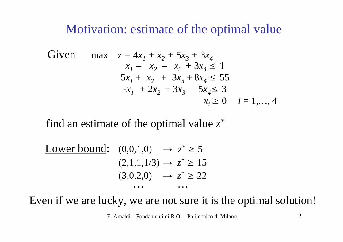
• By multiplying the 2° constraint by5/3we obtain aninequality thatdominatesthe objective function:
4x1 + x2 + 5x3 + 3x4 ≤ 25/3x1 + 5/3x2 + 5x3 + 40/3x4 ≤ 275/3 ∀ feasible solution
⇒ z* ≤ 275/3
• Adding 2° and 3° we obtain:
4x1 + 3x2 + 6x3 + 3x4 ≤ 58
⇒ z* ≤ 58 better upper bound
Upper bound:

E. Amaldi – Fondamenti di R.O. – Politecnico di Milano 4
General strategy: linearly combine the constraintswith nonnegativemultiplicative factors ( i-th constraintmultiplied byyi ≥ 0 )
first case: y1=0, y2=5/3, y3=0
second case: y1=0, y2=1, y3=1
In general
y1(x1 – x2 – x3 +3x4) + y2(5x1 + x2 + 3x3 + 8x4)
+ y3(-x1 + 2x2 + 3x3 – 5x4) ≤ y1 + 55y2 + 3y3

E. Amaldi – Fondamenti di R.O. – Politecnico di Milano 5
which is equivalent to:
(y1 + 5y2 – y3) x1 + (-y1 + y2 + 2y3) x2 + (-y1 + 3y2 + 3y3) x3
+ (3y1 + 8y2 – 5y3) x4 ≤ y1 + 55y2 + 3y3
NB: yi ≥ 0 so that the inequality direction is unchanged
(*)
In order to use the left hand side of (*) as upper bound on
z = 4x1 + x2 + 5x3 + 3x4
E. Amaldi – Fondamenti di R.O. – Politecnico di Milano 6
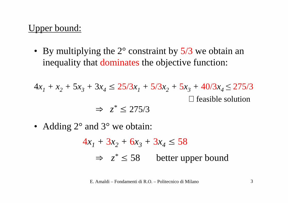
z = 4x1 + x2 + 5x3 + 3x4
We must have
y1 + 5y2 – y3≥ 4-y1 + y2 + 2y3 ≥ 1-y1 + 3y2 + 3y3 ≥ 53y1 + 8y2 –5y3 ≥ 3 yi ≥ 0, i = 1, 2, 3
In such a case, any feasible solution x satisfies
4x1 + x2 + 5x3 + 3x4 ≤ y1 + 55y2 + 3y3
in particular: z*≤ y1 + 55y2 + 3y3
E. Amaldi – Fondamenti di R.O. – Politecnico di Milano 7
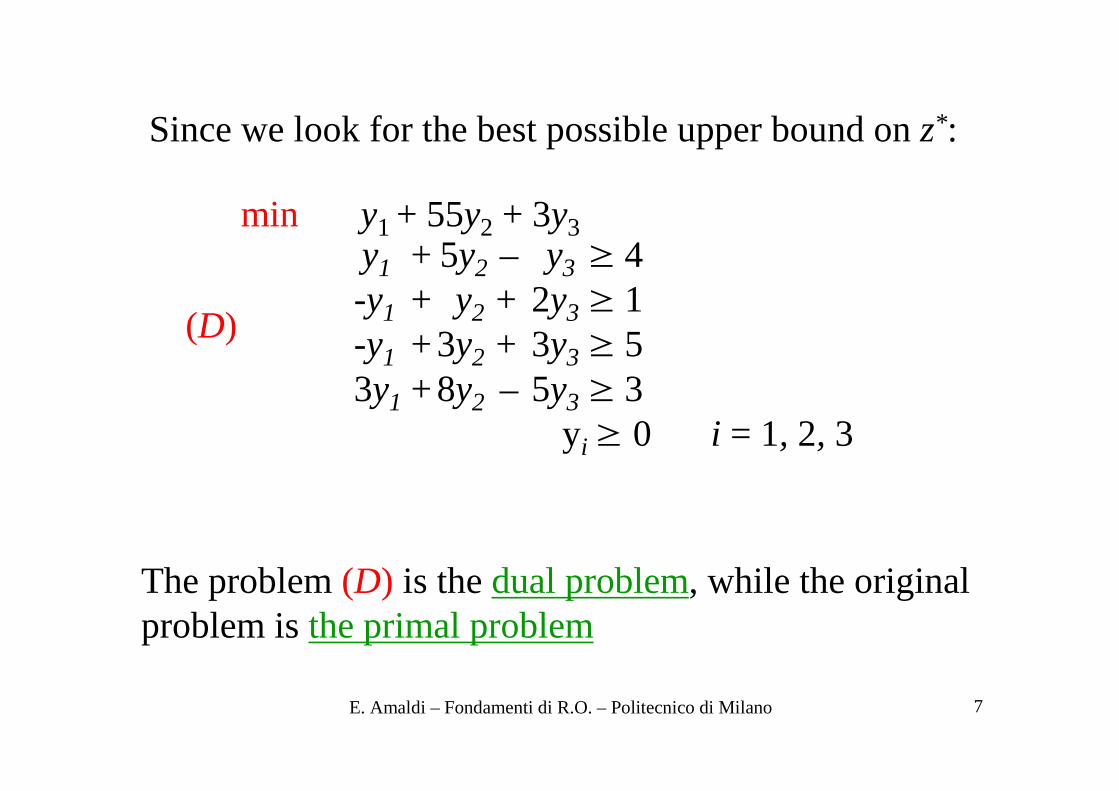
min y1 + 55y2 + 3y3y1 + 5y2 – y3 ≥ 4-y1 + y2 + 2y3 ≥ 1-y1 + 3y2 + 3y3 ≥ 53y1 + 8y2 – 5y3 ≥ 3
yi ≥ 0 i = 1, 2, 3
(D)
The problem(D) is the dual problem, while the originalproblemis the primal problem
Since we look for the best possible upper bound on z*:

E. Amaldi – Fondamenti di R.O. – Politecnico di Milano 8
max z = cTx
Ax≤ bx ≥ 0
(P)Primal
min w = bTy
ATy ≥ cy ≥ 0
(D)Dual o yTA ≥ cT
In matrix form:

E. Amaldi – Fondamenti di R.O. – Politecnico di Milano 9
Dual problem
min w = bTy
ATy ≥ cy ≥ 0
(D)
max z = cTx
Ax≤ bx ≥ 0
(P)
Dual of an LP in standard form?min z = cTx
Ax= bx ≥ 0

E. Amaldi – Fondamenti di R.O. – Politecnico di Milano 10
Standard form:
min z = cTx
Ax= bx ≥ 0
(P) ≡
max -cTx
x ≤
x ≥ 0
A’x ≤ b’A b-A -b
with A an m×n matrix ≡
y1
y2min (bT – bT)
(AT – AT) ≥ -c
y1 ≥ 0 , y2 ≥ 0
y1
y2
y1
y2y’ =
A’T
dual

E. Amaldi – Fondamenti di R.O. – Politecnico di Milano 11
max w = bTy
ATy ≤ cy ∈ Rm
(D)
≡
min -bT(y2 – y1)
-AT(y2 – y1) ≥ -c
y1 ≥ 0 , y2 ≥ 0
≡
y ≔ y2 – y1
unrestricted in sign!
min (bT – bT)
(AT – AT) ≥ -c
y1 ≥ 0 , y2 ≥ 0
y1
y2
y1
y2

E. Amaldi – Fondamenti di R.O. – Politecnico di Milano 12
max x1 + x2
x1 - x2 ≤ 2- 3x1 - 2x2 ≤ -12
x1, x2 ≥ 0
min 2y1 - 12y2
y1 - 3y2 ≥ 1-y1 - 2y2 ≥ 1
y1, y2 ≥ 0dual
max x1 + x2x1 – x2 ≤ 2
3x1+ 2x2 ≥ 12x1, x2 ≥ 0
(P)
Example:

E. Amaldi – Fondamenti di R.O. – Politecnico di Milano 13
General transformation rules
Primal (min) Dual (max)
mconstraints
n variables
coefficients obj. fct
right hand side
A
equality constraints
unrestriced variables
inequality constraints≥ (≤)
variables≥0 (≤0)
mvariables
n constraints
right hand side
coefficients obj. fct
AT
unrestriced variables
equality constraints
variables≥0 (≤0)
inequality constraints≤ (≥)

E. Amaldi – Fondamenti di R.O. – Politecnico di Milano 14
Example: using the above rules
min 2y1 + 12y2y1 + 3y2 ≥1-y1 + 2y2 ≥1y1 ≥ 0, y2 ≤ 0
max x1 + x2x1 – x2 ≤ 2
3x1 + 2x2 ≥ 12x1, x2 ≥ 0
(P)dual
min 2y1 - 12y2y1 - 3y2 ≥1
- y1 - 2y2 ≥1y1 ≥ 0, y2 ≥ 0
~~~
~
y1 ≔ -y1~

E. Amaldi – Fondamenti di R.O. – Politecnico di Milano 15
Exercize:
min 10x1 + 20x2 + 30x3
2x1 – x2 ≥ 1x2 + x3 ≤ 2
x1 – x3 = 3
x1 ≥ 0, x2 ≤ 0, x3 unrestricted
(P)
Dual?
E. Amaldi – Fondamenti di R.O. – Politecnico di Milano 16
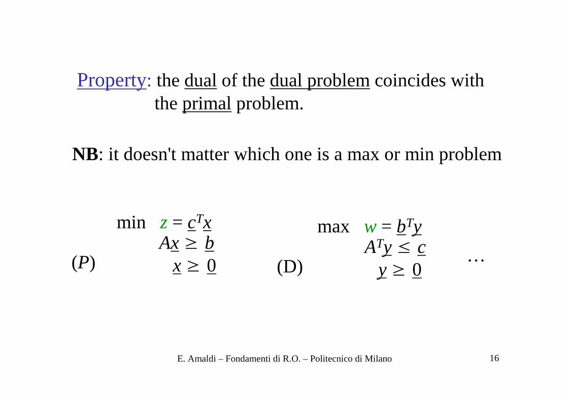
Property: the dualof the dual problemcoincides withthe primalproblem.
NB: it doesn't matter which one is a max or min problem
max w = bTyATy ≤ c
y ≥ 0(D)
min z = cTxAx≥ b
x ≥ 0(P) …
E. Amaldi – Fondamenti di R.O. – Politecnico di Milano 17
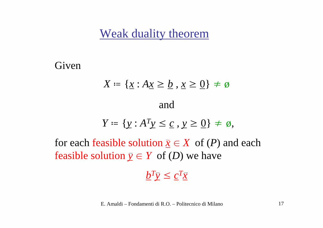
Weak duality theorem
Given
X ≔ { x : Ax≥ b , x≥ 0} ≠ ø
and
Y ≔ { y : ATy ≤ c , y≥ 0} ≠ ø,
for eachfeasible solutionx ∈ X of (P) and eachfeasible solutiony ∈ Y of (D) we have
bTy ≤ cTx

E. Amaldi – Fondamenti di R.O. – Politecnico di Milano 18
Given x ∈ X and y ∈ Y, we haveAx≥ b , x≥ 0 and
ATy ≤ c, y≥ 0 which imply that
Proof
xTAT c
≤
≤
bTy ≤ xTATy ≤ xTc = cTx
E. Amaldi – Fondamenti di R.O. – Politecnico di Milano 19
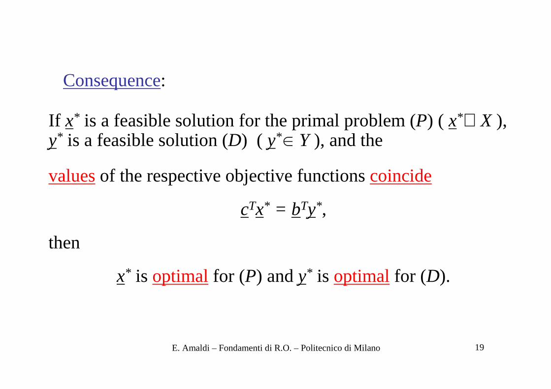
If x* is a feasible solution for the primal problem (P) ( x*∈ X ), y* is a feasible solution (D) ( y*
∈ Y ), and the
valuesof the respective objective functionscoincide
cTx* = bTy*,
then
x* is optimalfor (P) and y* is optimalfor (D).
Consequence:

E. Amaldi – Fondamenti di R.O. – Politecnico di Milano 20
Strong duality theorem
If X = { x : Ax≥ b , x≥ 0} ≠ ø and min{ cTx : x ∈ X} isfinite, there exist x*
∈ X andy*∈ Y such thatcTx* = bTy* .
optimummin{ cTx : x ∈ X } = max{ bTy : y ∈ Y }
z* = w*
w = bTy y ∈ Y feasible for (D)
z = cTx x ∈ X feasible for (P)

E. Amaldi – Fondamenti di R.O. – Politecnico di Milano 21
Derive an optimal solution of (D) from one of (P)
max yTb
yTA ≤ cT
y ∈ Rm
(D)
min cTx
Ax= bx ≥ 0
(P)
Given
and x* is an optimal feasible solution of (P)
x* = conx*
Bx*
N
x*B = B-1b
x*N = 0
provided (after a finite # of iterations) by the Simplex algorithmwith Bland's rule.
Proof
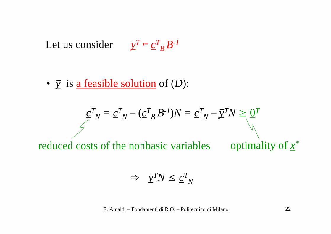
E. Amaldi – Fondamenti di R.O. – Politecnico di Milano 22
optimality of x*reduced costs of the nonbasic variables
• y is a feasible solutionof (D):
Let us consider yT ≔ cTB B-1
cTN = cT
N – (cTB B-1)N = cT
N – yTN ≥ 0T
⇒ yTN ≤ cTN

E. Amaldi – Fondamenti di R.O. – Politecnico di Milano 23
reduced costs of the basic variables
I
cTB = cT
B – (cTB B-1)B = cT
B – yTB = 0T ⇒ yTB ≤ cTB
• y is anoptimal solutionof (D):
yTb = (cTB B-1)b = cT
B (B-1b) = cTB x*
B = cTx*
hencey = y*

E. Amaldi – Fondamenti di R.O. – Politecnico di Milano 24
Corollary
For any pair of primal-dual problems (P) and (D), only four cases can arise:
∃ optimal
solutionunbounded
LP infeasible
LP
∃ optimal
solution
unbounded LP
InfeasibleLP
P
D
1)
2)
3) 4)

E. Amaldi – Fondamenti di R.O. – Politecnico di Milano 25
Strong duality theorem ⇒ 1)
Weak duality theorem ⇒ 2) and 3)
4) can arise:
empty feasible regions
min -4x1 – 2x2-x1 + x2 ≥ 2x1 – x2 ≥ 1
x1, x2 ≥ 0
(P)
max 2y1 + y2-y1 + y2 ≤ -4y1 – y2 ≤ -2
y1, y2 ≥ 0
(D)

E. Amaldi – Fondamenti di R.O. – Politecnico di Milano 26
Economic interpretation
The primal and dual problems correspond to two complementary point of views on the same “market”
Diet problem:
n aliments j= 1,…, n
m nutrients i= 1,…, m (vitamines,…)
aij quantity of i-th nutrient in one unit of j-th aliment
bi requirement of i-th nutrient
cj cost of one unit of j-th aliment
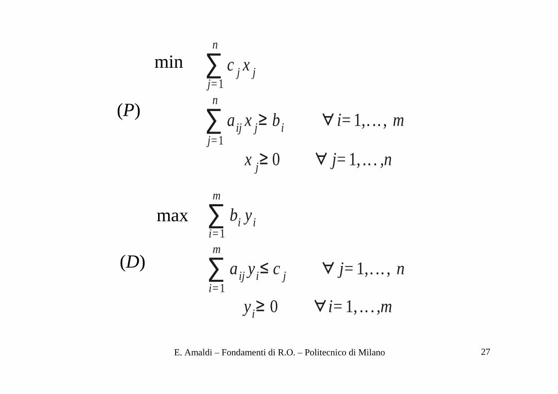
E. Amaldi – Fondamenti di R.O. – Politecnico di Milano 27
∑j= 1
n
c j x j
∑j= 1
n
aij x j≥ bi ∀i= 1,. .. , m
x j≥ 0 ∀ j= 1, .. .,n
(P)
(D)
min
max ∑i= 1
m
bi yi
∑i= 1
m
aij yi≤ c j ∀ j= 1,. .. , n
yi≥ 0 ∀i= 1, .. .,m

E. Amaldi – Fondamenti di R.O. – Politecnico di Milano 28
Interpretation of the dual problem: A company that produces pills of the mnutrients needs todecide the nutrient unit pricesyi so as to maximize income.
• If the costumer buys nutrient pills he will buy bi units for each i, 1 ≤ i ≤m
• The price of the nutrient pills must be competitive:
∑i= 1
m
aij yi≤ c j ∀ j= 1,. ..,n
cost of the pills that are equivalent to 1 unit of j-th aliment

E. Amaldi – Fondamenti di R.O. – Politecnico di Milano 29
If both linear programs (P) and (D) admit a feasiblesolution, the strong duality theoremimplies that
z* = w*
An “equilibrium” exists (two alternatives with the same cost)
NB: Strong connection with Game theory (zero-sum games)
E. Amaldi – Fondamenti di R.O. – Politecnico di Milano 30
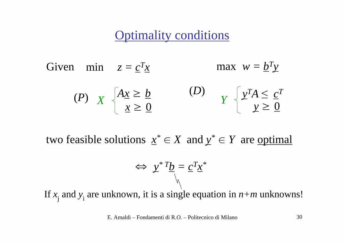
Optimality conditions
Given min z = cTx
Ax≥ bx ≥ 0
(P) X
max w = bTy
yTA ≤ cT
y ≥ 0(D)
Y
two feasible solutionsx*∈ X and y*
∈ Y are optimal
⇔ y* Tb = cTx*
If xj and yi are unknown, it is a single equation inn+m unknowns!

E. Amaldi – Fondamenti di R.O. – Politecnico di Milano 31
Since y*Tb ≤ y*TAx* ≤ cTx*, we have
y*Tb = y*TAx* and y*TAx* = cTx*
≤
Ax*
≤
cT
therefore
y*T (Ax* - b) = 0 and (cT - y*TA) x* = 0
0T 0 0T 0
necessaryand sufficientoptimality conditions!
⇒ m+n equations inn+m unknowns
≤ ≤ ≤
≤

E. Amaldi – Fondamenti di R.O. – Politecnico di Milano 32
Complementary slackness conditions
x*∈ X and y*
∈ Y are optimal solutionsof, respectively, (P) and (D) if and only if
y*i (aT
i x* - bi) = 0 ∀ i = 1,…, m
(cTj – y*TAj) x*
j = 0 ∀ j = 1,…, n
i-th row of A
j-th column of A
At optimality, the productof each variablewith the corresponding slack variableof the relative dualis = 0.
slack ofj-th constraint of (D)
slack si of i-th constraint of (P)

E. Amaldi – Fondamenti di R.O. – Politecnico di Milano 33
Economic interpretation for the diet problem
If the optimal diet includes an excess of i-th nutrient, the costumer is not willing to payy*
i > 0
If the company selects a price y*i > 0, the costumer
must not have an excess of i-th nutrient
0 *
1
* =⇒>∑•=
ii
n
jjij ybxa
i
n
jjiji bxay =∑⇒>•
=1
** 0

E. Amaldi – Fondamenti di R.O. – Politecnico di Milano 34
price of the pills equivalent to the nutrients contained in one unit of j-th alimentis lower than the price of the aliment
If costumer includes the j-th aliment in optimal diet, the company must have selected competitive pricesy*
i
(the price of the nutrients in pills contained in a unit of j-th aliment is not lower thancj )
it is not convenient for the costumer to buy aliment j
0 *
1
* =⇒<∑•=
jj
m
iiji xcay
j
m
iijij cayx =∑⇒>•
=1
** 0
E. Amaldi – Fondamenti di R.O. – Politecnico di Milano 35
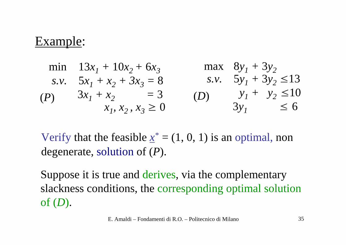
Example:
max 8y1 + 3y2s.v. 5y1 + 3y2 ≤13
y1 + y2 ≤103y1 ≤ 6
min 13x1 + 10x2 + 6x3
s.v. 5x1 + x2 + 3x3 = 83x1 + x2 = 3
x1, x2 , x3 ≥ 0(P) (D)
Verify that the feasiblex* = (1, 0, 1) is an optimal,non degenerate, solutionof (P).
Suppose it is true and derives, via the complementaryslackness conditions, the corresponding optimal solutionof (D).
E. Amaldi – Fondamenti di R.O. – Politecnico di Milano 36
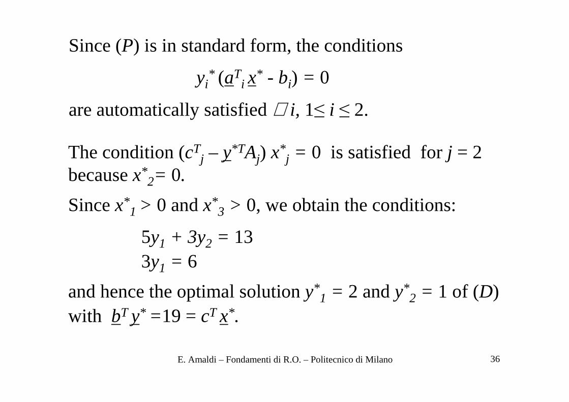
Since (P) is in standard form, the conditions
yi* (aT
i x* - bi) = 0
are automatically satisfied∀ i, 1≤ i ≤ 2.
The condition (cTj – y*TAj) x*
j = 0 is satisfied forj = 2 because x*
2= 0.
Sincex*1 > 0 and x*
3 > 0, we obtain the conditions:
5y1 + 3y2 = 133y1 = 6
and hence the optimal solution y*1 = 2 and y*
2 = 1 of (D) with bT y* =19 = cT x*.