4.3 Double Integrals Over General Regions - KSU Web...
24
4.3. DOUBLE INTEGRALS OVER GENERAL REGIONS 323 Figure 4.7: Bounded region in R 2 4.3 Double Integrals Over General Regions 4.3.1 Introduction When dealing with integrals of functions of one variable, we are always inte- grating over an interval. The only di¢ culty in evaluating the denite integral R b a f (x) dx came from the function f and the di¢ culty to nd an antiderivative for it. With functions of two or more variables, not only the function can cause the integral to be di¢ cult, but also the region over which we integrate. In the previous section, we restricted ourselves to rectangular regions. However, not every region is rectangular. A region of R 2 can have any shape. Even if the function is easy to integrate, if the region is complex enough, the integral will still be di¢ cult to evaluate. We rst dene the integral of a function over two variables over a general region. We will then show how this integral can be evaluated over some simple regions which we will call regions of types I and II. Let us assume we are given a function f (x; y) dened on a closed and bounded region D as shown in gure 4.7. Suppose we want to integrate f over D. Because D is bounded, it can be enclosed in a rectangle R as shown in gure 4.8. To dene the integral of f over D, we rst dene the function F (x; y) as follows: F (x; y)= f (x; y) if (x; y) 2 D 0 if (x; y) 2 R D (4.3)
Transcript of 4.3 Double Integrals Over General Regions - KSU Web...
4.3. DOUBLE INTEGRALS OVER GENERAL REGIONS 323
Figure 4.7: Bounded region in R2
4.3 Double Integrals Over General Regions
4.3.1 Introduction
When dealing with integrals of functions of one variable, we are always inte-grating over an interval. The only diffi culty in evaluating the definite integral∫ baf (x) dx came from the function f and the diffi culty to find an antiderivative
for it. With functions of two or more variables, not only the function can causethe integral to be diffi cult, but also the region over which we integrate. In theprevious section, we restricted ourselves to rectangular regions. However, notevery region is rectangular. A region of R2 can have any shape. Even if thefunction is easy to integrate, if the region is complex enough, the integral willstill be diffi cult to evaluate. We first define the integral of a function over twovariables over a general region. We will then show how this integral can beevaluated over some simple regions which we will call regions of types I and II.
Let us assume we are given a function f (x, y) defined on a closed andbounded region D as shown in figure 4.7. Suppose we want to integrate fover D. Because D is bounded, it can be enclosed in a rectangle R as shown infigure 4.8.
To define the integral of f over D, we first define the function F (x, y) asfollows:
F (x, y) =
f (x, y) if (x, y) ∈ D0 if (x, y) ∈ R−D (4.3)
324 CHAPTER 4. MULTIPLE INTEGRALS
Figure 4.8: Bounded region in R2, enclosed in a rectangle.
Definition 4.3.1 If∫∫R
F (x, y) dA exists, then we define
∫∫D
f (x, y) dA =
∫∫R
F (x, y) dA
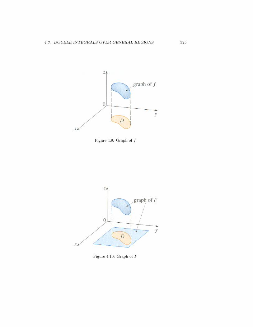
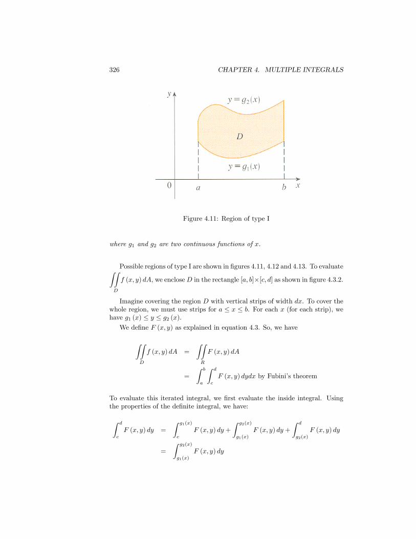
This definition makes sense since, as we can see in figures 4.9 and 4.10, theportion of the graph of F which is not 0 is identical to the graph of f. Theportion which is 0 will not contribute to the integral. In particular, this meansthat for our definition, it does not matter which rectangle R we select. In the
case, f (x, y) ≥ 0,∫∫D
f (x, y) dA corresponds to the volume of the solid which
lies above D and below the graph of z = f (x, y).
We still must be able to compute∫∫R
F (x, y) dA. This is not always a simple
task. But it is for certain regions, which we consider next.
4.3.2 Regions of Type I
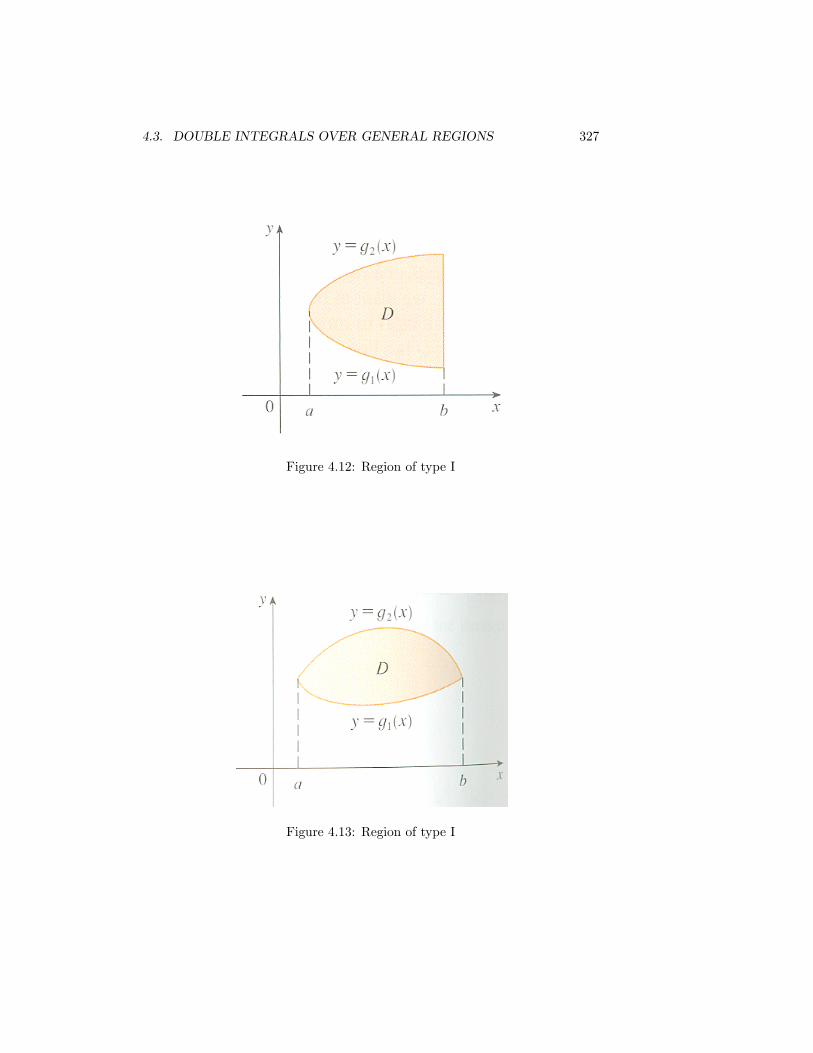
When describing a region, one has to give the condition x and y must satisfyso that a point (x, y) lies in the region. A region is said to be of type I if x isbetween two constants, and y is between two continuous functions of x. Moreprecisely, we have the following definition:
Definition 4.3.2 A plane region D is said to be of type I if it is of the form
D =
(x, y) ∈ R2 | a ≤ x ≤ b and g1 (x) ≤ y ≤ g2 (x)
4.3. DOUBLE INTEGRALS OVER GENERAL REGIONS 325
Figure 4.9: Graph of f
Figure 4.10: Graph of F
326 CHAPTER 4. MULTIPLE INTEGRALS
Figure 4.11: Region of type I
where g1 and g2 are two continuous functions of x.
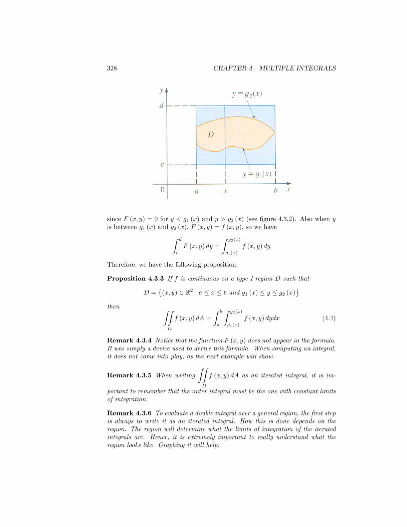
Possible regions of type I are shown in figures 4.11, 4.12 and 4.13. To evaluate∫∫D
f (x, y) dA, we encloseD in the rectangle [a, b]×[c, d] as shown in figure 4.3.2.
Imagine covering the region D with vertical strips of width dx. To cover thewhole region, we must use strips for a ≤ x ≤ b. For each x (for each strip), wehave g1 (x) ≤ y ≤ g2 (x).
We define F (x, y) as explained in equation 4.3. So, we have
∫∫D
f (x, y) dA =
∫∫R
F (x, y) dA
=
∫ b
a
∫ d
c
F (x, y) dydx by Fubini’s theorem
To evaluate this iterated integral, we first evaluate the inside integral. Usingthe properties of the definite integral, we have:
∫ d
c
F (x, y) dy =
∫ g1(x)
c
F (x, y) dy +
∫ g2(x)
g1(x)
F (x, y) dy +
∫ d
g2(x)
F (x, y) dy
=
∫ g2(x)
g1(x)
F (x, y) dy
4.3. DOUBLE INTEGRALS OVER GENERAL REGIONS 327
Figure 4.12: Region of type I
Figure 4.13: Region of type I
328 CHAPTER 4. MULTIPLE INTEGRALS
since F (x, y) = 0 for y < g1 (x) and y > g2 (x) (see figure 4.3.2). Also when yis between g1 (x) and g2 (x), F (x, y) = f (x, y), so we have∫ d
c
F (x, y) dy =
∫ g2(x)
g1(x)
f (x, y) dy
Therefore, we have the following proposition:
Proposition 4.3.3 If f is continuous on a type I region D such that
D =
(x, y) ∈ R2 | a ≤ x ≤ b and g1 (x) ≤ y ≤ g2 (x)
then ∫∫D
f (x, y) dA =
∫ b
a
∫ g2(x)
g1(x)
f (x, y) dydx (4.4)
Remark 4.3.4 Notice that the function F (x, y) does not appear in the formula.It was simply a device used to derive this formula. When computing an integral,it does not come into play, as the next example will show.
Remark 4.3.5 When writing∫∫D
f (x, y) dA as an iterated integral, it is im-
portant to remember that the outer integral must be the one with constant limitsof integration.
Remark 4.3.6 To evaluate a double integral over a general region, the first stepis always to write it as an iterated integral. How this is done depends on theregion. The region will determine what the limits of integration of the iteratedintegrals are. Hence, it is extremely important to really understand what theregion looks like. Graphing it will help.
4.3. DOUBLE INTEGRALS OVER GENERAL REGIONS 329
Example 4.3.7 Write∫∫D
f (x, y) dA as an iterated integral where D =
(x, y) ∈ R2 | 0 ≤ x ≤ 1 and − x2 ≤ y ≤ x2
Here, the region is given explicitly, we know the limits for both x and y, so wecan write the iterated integral.
∫∫D
f (x, y) dA =
∫ 1
0
∫ x2
−x2f (x, y) dydx
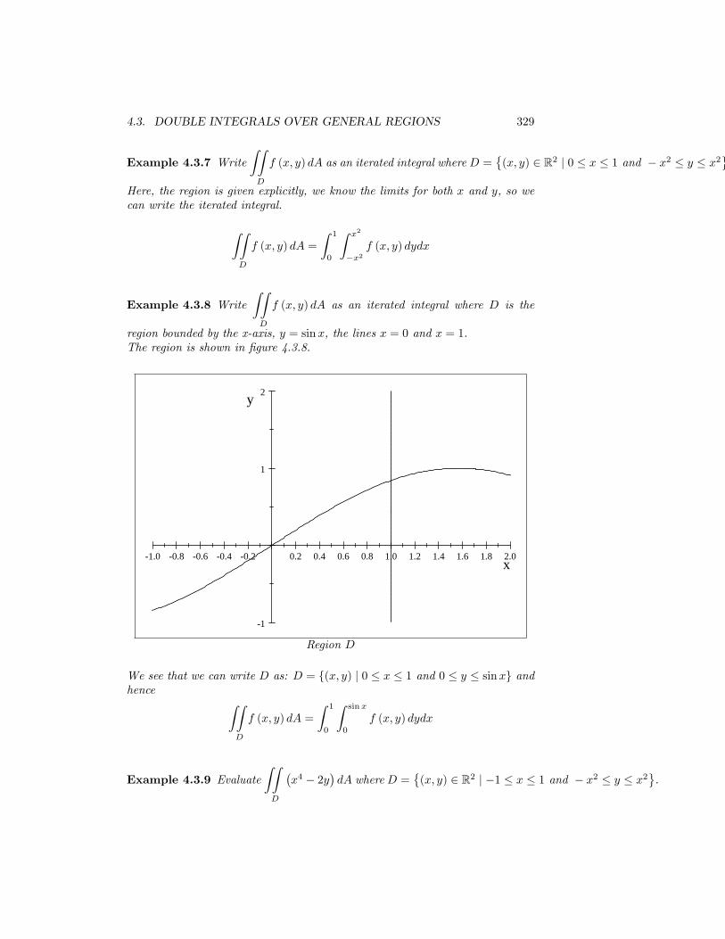
Example 4.3.8 Write∫∫D
f (x, y) dA as an iterated integral where D is the
region bounded by the x-axis, y = sinx, the lines x = 0 and x = 1.The region is shown in figure 4.3.8.
1.0 0.8 0.6 0.4 0.2 0.2 0.4 0.6 0.8 1.0 1.2 1.4 1.6 1.8 2.0
1
1
2
x
y
Region D
We see that we can write D as: D = (x, y) | 0 ≤ x ≤ 1 and 0 ≤ y ≤ sinx andhence ∫∫
D
f (x, y) dA =
∫ 1
0
∫ sin x
0
f (x, y) dydx
Example 4.3.9 Evaluate∫∫D
(x4 − 2y
)dA where D =
(x, y) ∈ R2 | −1 ≤ x ≤ 1 and − x2 ≤ y ≤ x2
.
330 CHAPTER 4. MULTIPLE INTEGRALS
D is clearly a type I region.∫∫D
(x4 − 2y
)dA =
∫ 1
−1
∫ x2
−x2
(x4 − 2y
)dydx
=
∫ 1
−1
[x4y − y2
∣∣x2−x2
]dx
=
∫ 1
−1
(x6 − x4 + x6 + x4
)dx
=
∫ 1
−1
2x6dx
=2
7x7
∣∣∣∣1−1
=4
7
4.3.3 Regions of Type II
The condition a point (x, y) must satisfy to be in a type II region is as follows.A region is said to be of type II if y is between two constants, and x is betweentwo continuous functions of y. More precisely, we have the following definition:
Definition 4.3.10 A plane region D is said to be of type II if it is of the form
D =
(x, y) ∈ R2 | c ≤ y ≤ d and h1 (y) ≤ x ≤ h2 (y)
Using the same method as for type I regions, we can show that
Proposition 4.3.11 If f is continuous on a type II region D such that
D =
(x, y) ∈ R2 | c ≤ y ≤ d and h1 (y) ≤ x ≤ h2 (y)
then ∫∫D
f (x, y) dA =
∫ d
c
∫ h2(y)
h1(y)
f (x, y) dxdy (4.5)
Remark 4.3.12 This time, we imagine covering the region D with horizontalstrips of height dy. To cover the whole region, we must use strips for c ≤ y ≤ d.For each y (for each strip), we have h1 (y) ≤ x ≤ h2 (y).
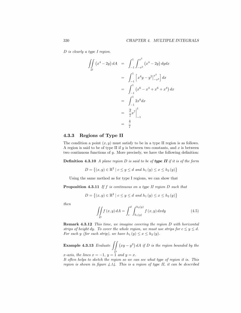
Example 4.3.13 Evaluate∫∫D
(xy − y3
)dA if D is the region bounded by the
x-axis, the lines x = −1, y = 1 and y = x.It often helps to sketch the region so we can see what type of region it is. Thisregion is shown in figure 4.14. This is a region of type II, it can be described
4.3. DOUBLE INTEGRALS OVER GENERAL REGIONS 331
Figure 4.14: Region bouded by the x−axis, and the lines y = −1, x = −1, andy = x.
by D =
(x, y) ∈ R2 | 0 ≤ y ≤ 1 and − 1 ≤ x ≤ y. In type II regions, x is the
variable between two functions of y. Make sure these are functions of y, not x.In this case, the right side of the region is delimited by the line y = x, whichwhen we write as a function of y becomes x = y. Therefore, we have∫∫
D
(xy − y3
)dA =
∫ 1
0
∫ y
−1
(xy − y3
)dxdy
=
∫ 1
0
[x2
2y − xy3
∣∣∣∣y−1
]dy
=
∫ 1
0
(y3
2− y4 −
(y2
+ y3))
dy
=
∫ 1
0
(−y4 − y3
2− y
2
)dy
=
(−y
5
5− y4
8− y2
4
)∣∣∣∣10
= −23
40
4.3.4 Properties
We list without proof several properties the double integral satisfies. Theseproperties are very similar to the properties of the definite integral of functionsof one variable.
Proposition 4.3.14 Assuming that the following integrals exist and that C isa constant, we have:
332 CHAPTER 4. MULTIPLE INTEGRALS
1.∫∫D
(f (x, y)± g (x, y)) dA =
∫∫D
f (x, y) dA±∫∫D
g (x, y) dA
2.∫∫D
Cf (x, y) dA = C
∫∫D
f (x, y) dA
3. If f (x, y) ≥ g (x, y) for all (x, y) in D, then∫∫D
f (x, y) dA ≥∫∫D
g (x, y) dA
Proposition 4.3.15 If D, D1 and D2 are three regions in R2 such that D =D1 ∪D2 and D1 and D2 do not overlap then∫∫
D
f (x, y) dA =
∫∫D1
f (x, y) dA+
∫∫D2
f (x, y) dA
This property corresponds to the property for functions of one variable whichsays:
∫ baf (x) dx =
∫ caf (x) dx+
∫ bcf (x) dx. It can sometimes be used to evalu-
ate integrals over regions which are neither of type I, nor of type II. If we havesuch a region and we can divide it into two (or more regions) of type I or II ,then we can break the integral into integrals over the subregions. Each integralis then an integral of type I or II, which we know how to evaluate.
Proposition 4.3.16∫∫D
1dA = A (D) where A (D) denotes the area of D.
This property says that if we integrate the constant function f (x, y) = 1over a region D, we get the area of D. This makes sense. The volume of a solida section D between two parallel planes is (area of the section)×height. In thiscase, the height is simply 1. This is also very important as it gives us a way ofcomputing the area of general regions. We illustrate it with an example.
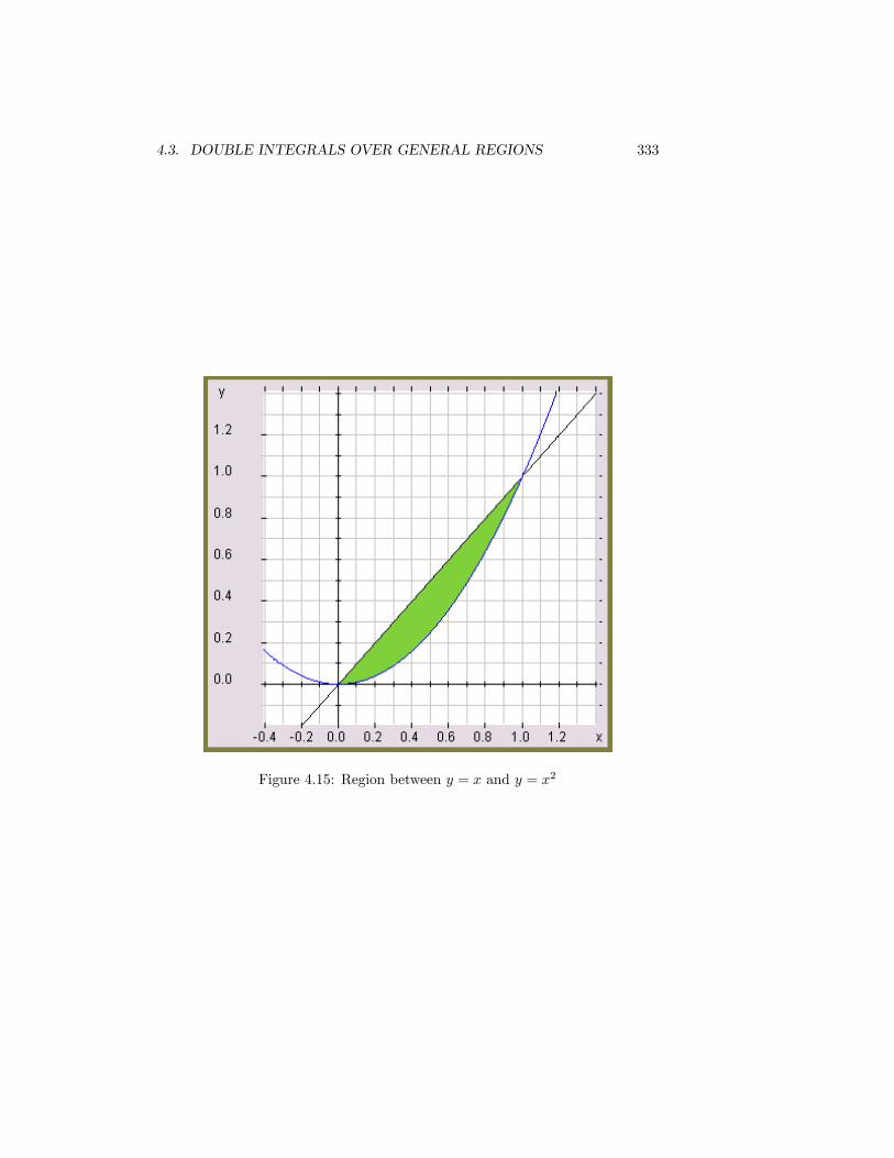
Example 4.3.17 Find the area of the region D in the first quadrant boundedby y = x and y = x2.The region is shown in figure 4.15. We can treat this as a type 1 or a type 2region. We show the solution both ways.
• Type 1 region. The area of the region is∫∫D
dA where D is the region
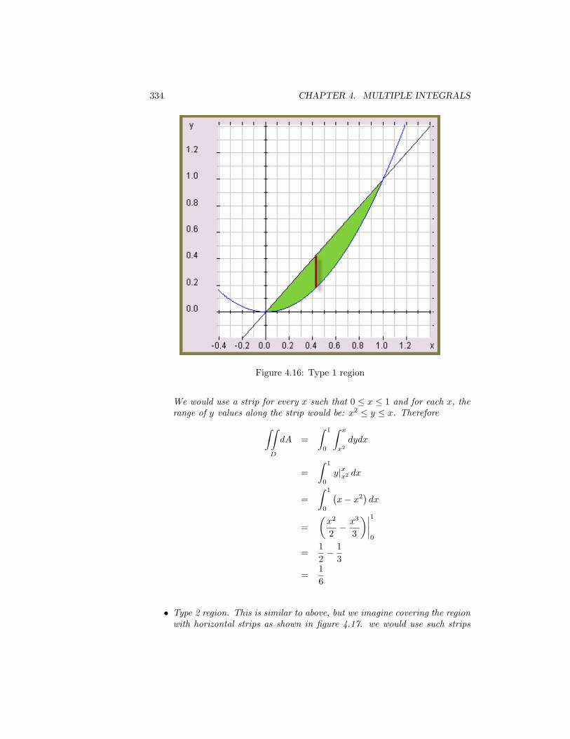
described in the problem, in green on figure 4.15. To evaluate this integral,we must rewrite it as an iterated integral treating D as a type 1 region. Weimagine covering the region with vertical strips as shown in figure 4.16.
4.3. DOUBLE INTEGRALS OVER GENERAL REGIONS 333
Figure 4.15: Region between y = x and y = x2
334 CHAPTER 4. MULTIPLE INTEGRALS
Figure 4.16: Type 1 region
We would use a strip for every x such that 0 ≤ x ≤ 1 and for each x, therange of y values along the strip would be: x2 ≤ y ≤ x. Therefore∫∫
D
dA =
∫ 1
0
∫ x
x2dydx
=
∫ 1
0
y|xx2 dx
=
∫ 1
0
(x− x2
)dx
=
(x2
2− x3
3
)∣∣∣∣10
=1
2− 1
3
=1
6
• Type 2 region. This is similar to above, but we imagine covering the regionwith horizontal strips as shown in figure 4.17. we would use such strips
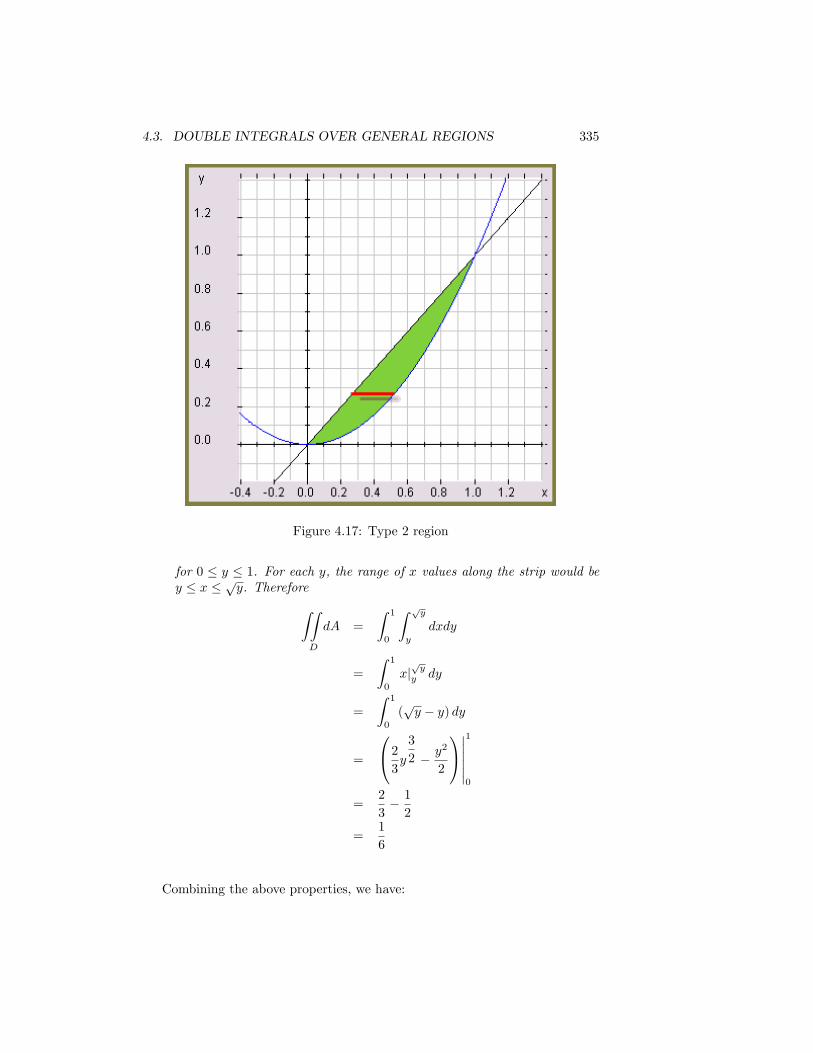
4.3. DOUBLE INTEGRALS OVER GENERAL REGIONS 335
Figure 4.17: Type 2 region
for 0 ≤ y ≤ 1. For each y, the range of x values along the strip would bey ≤ x ≤ √y. Therefore∫∫
D
dA =
∫ 1
0
∫ √yy
dxdy
=
∫ 1
0
x|√y
y dy
=
∫ 1
0
(√y − y) dy
=
2
3y
3
2 − y2
2
∣∣∣∣∣∣1
0
=2
3− 1
2
=1
6
Combining the above properties, we have:
336 CHAPTER 4. MULTIPLE INTEGRALS
Figure 4.18: Region bounded by y = x2 and y = 4√x
Proposition 4.3.18 If m ≤ f (x, y) ≤M for all (x, y) in D, then
mA (D) ≤∫∫D
f (x, y) dA ≤MA (D)
Definition 4.3.19 (Average Value) We define the average value of a func-tion f (x, y) over a region D to be
Average value of f over D =1
area of D
∫∫D
f (x, y) dA
4.3.5 More Practice Problems
In many cases, a region can be considered of type I or II. One then has to decidewhether to treat it as a type I region or a type II. It may be that either way willwork. However, in some cases, one way may lead to an integral which is verydiffi cult, while the other way leads to an easier integral. In the example thatfollows, we look at cases to illustrate these various options. The more problemyou practice on, the better you will become at identifying the type of a region,and how to perform the integration.
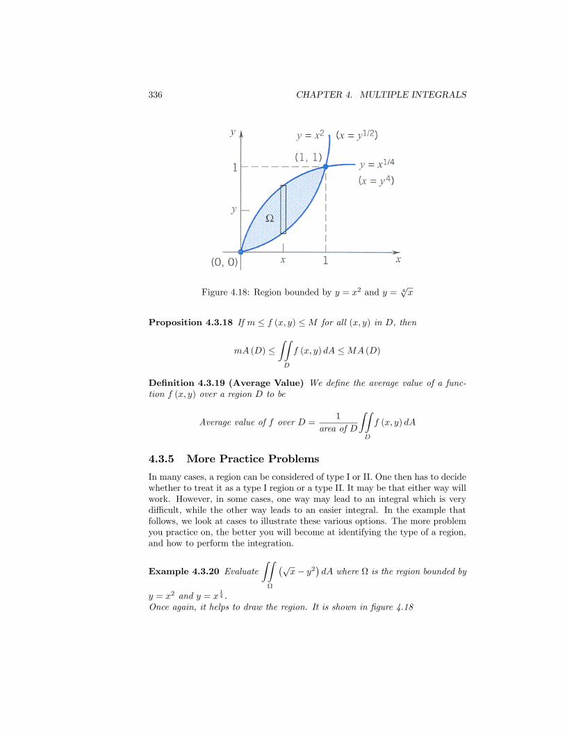
Example 4.3.20 Evaluate∫∫
Ω
(√x− y2
)dA where Ω is the region bounded by
y = x2 and y = x14 .
Once again, it helps to draw the region. It is shown in figure 4.18
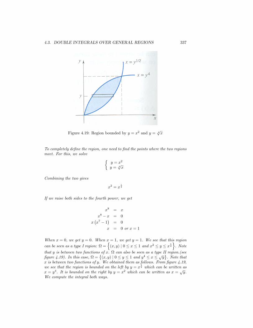
4.3. DOUBLE INTEGRALS OVER GENERAL REGIONS 337
Figure 4.19: Region bounded by y = x2 and y = 4√x
To completely define the region, one need to find the points where the two regionsmeet. For this, we solve
y = x2
y = 4√x
Combining the two gives
x2 = x14
If we raise both sides to the fourth power, we get
x8 = x
x8 − x = 0
x(x7 − 1
)= 0
x = 0 or x = 1
When x = 0, we get y = 0. When x = 1, we get y = 1. We see that this region
can be seen as a type I region: Ω =
(x, y) | 0 ≤ x ≤ 1 and x2 ≤ y ≤ x 14
. Note
that y is between two functions of x. Ω can also be seen as a type II region.(seefigure 4.19). In this case, Ω =
(x, y) | 0 ≤ y ≤ 1 and y4 ≤ x ≤ √y
. Note that
x is between two functions of y. We obtained them as follows. From figure 4.19,we see that the region is bounded on the left by y = x
14 which can be written as
x = y4. It is bounded on the right by y = x2 which can be written as x =√y.
We compute the integral both ways.
338 CHAPTER 4. MULTIPLE INTEGRALS
Method 1 Treating Ω as a type I region.
∫∫Ω
(√x− y2
)dA =
∫ 1
0
∫ x14
x2
(√x− y2
)dydx
=
∫ 1
0
y√x− y3
3
∣∣∣∣x14
x2
dx=
∫ 1
0
((x34 − x
34
3
)−(x52 − x6
3
))dx
=
∫ 1
0
(2
3x34 − x 5
2 +x6
3
)dx
=
(8
21x74 − 2
7x72 +
x7
21
)∣∣∣∣10
=8
21− 2
7+
1
21
=1
7
Method 2 Treating Ω as a type II region.
∫∫Ω
(√x− y2
)dA =
∫ 1
0
∫ y12
y4
(√x− y2
)dxdy
=
∫ 1
0
(2
3x32 − xy2
)∣∣∣∣y12
y4
dy=
∫ 1
0
((2
3y34 − y 5
2
)−(
2
3y6 − y6
))dy
=
∫ 1
0
(2
3y34 − y 5
2 +y6
3
)dy
=
((8
21y74 − 2
7y72 − y7
21
))∣∣∣∣10
=
(8
21− 2
7+
1
21
)=
1
7
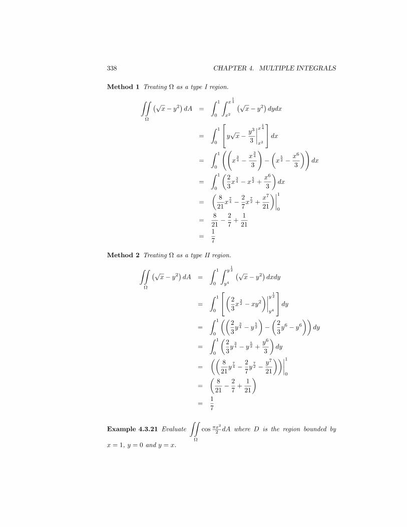
Example 4.3.21 Evaluate∫∫
Ω
cos πx2
2 dA where D is the region bounded by
x = 1, y = 0 and y = x.
4.3. DOUBLE INTEGRALS OVER GENERAL REGIONS 339
Figure 4.20: Region bounded by x = 0, x = 1, y = 0 and y = x
The region is shown in figure 4.20. Once again, we see that this region can betreated as a type I or type II region.
Method 1 Treating Ω as a type I region. The corner points of the region are(0, 0), (1, 0) and (1, 1). The region is determined by Ω = (x, y)0 ≤ x ≤ 1 and 0 ≤ y ≤ x.In this case: ∫∫
Ω
cosπx2
2dA =
∫ 1
0
∫ x
0
cosπx2
2dydx
=
∫ 1
0
[y cos
πx2
2
∣∣∣∣x0
]dx
=
∫ 1
0
x cosπx2
2dx
We finish with a substitution. If we let u = πx2
2 then du = πxdx. Also,when x = 0, u = 0 and when x = 1, u = π
2 . So, we have∫∫Ω
cosπx2
2dA =
1
π
∫ π2
0
cosudu
=1
π(sinu)|
π20
=1
π
Method 2 Treating Ω as a type II region. The region is determined by Ω =
340 CHAPTER 4. MULTIPLE INTEGRALS
(x, y) | 0 ≤ y ≤ 1 and y ≤ x ≤ 1. So∫∫Ω
cosπx2
2dA =
∫ 1
0
∫ 1
y
cosπx2
2dxdy
We cannot evaluate the inside integral as we do not know an antiderivativewith respect to x of
∫ 1
ycos πx
2
2 dx.
Example 4.3.22 Calculate the volume of the solid within the cylinder x2+y2 =b2, between the planes y + z = a and z = 0, given that a ≥ b > 0.The region is shown in figure 4.3.22. The region D in R2 by which the solid isbounded is D =
(x, y) | x2 + y2 ≤ b2
. The solid is also bounded by the planes
z = 0 and z = −y + a. Therefore, its volume is given by the integral∫∫D
(a− y) dA =
∫∫D
adA−∫∫D
ydA
The second integral is easier to evaluate than it seems. The region D can bewritten as
D =
(x, y) | −b ≤ x ≤ b and −√b2 − x2 ≤ y ≤
√b2 − x2
Thus, ∫∫
D
ydA =
∫ b
−b
∫ √b2−x2−√b2−x2
ydydx
You will recall that integrating an odd function over a symmetric integral gives0, in other words, if f (x) is an odd function, then
∫ a−a f (x) dx = 0. Thus,
4.3. DOUBLE INTEGRALS OVER GENERAL REGIONS 341
∫√b2−x2−√b2−x2 ydy = 0. It follows that∫∫
D
(a− y) dA =
∫∫D
adA
= a
∫∫D
dA
= aA (D) by one of the properties above
= πab2
4.3.6 Switching the Order of Integration
Evaluating a double integral over a region amounts to evaluating one or moreiterated integrals. As we know, there are two kinds of iterated integrals. Onein which the dx integral is the inner integral and the dy integral is the outerintegral. The other kind is the reverse. When the region of integration is arectangle, Fubini’s theorem tells us that the two integrals are the same. If R =
[a, b] × [c, d]. Then∫∫R
f (x, y) dA =∫ ba
∫ dcf (x, y) dydx =
∫ dc
∫ baf (x, y) dxdy.
When the region of integration is not a rectangle, we may not have a choice.We may be forced to use one of the iterated integrals as suggests example4.3.21. That example also suggests that given an iterated integral, to evaluateit might require switching the order of integration. This cannot be done by justreversing the order of the integrals. It involves changing the type of region weare integrating over. We illustrate this with an example.
Example 4.3.23 Switch the order of integration∫ 1
0
∫ 1
ycos πx
2
2 dxdy.First, we need to identify the region, decide what type of region it is. Then,we rewrite it as a region of the other type and write the integral in terms ofthat region. From the limits of integration, we see that the region is D =
(x, y) : 0 ≤ y ≤ 1 and y ≤ x ≤ 1. Thus, this is a type II region. Thus∫ 1
0
∫ 1
ycos πx
2
2 dxdy =∫∫D
cos πx2
2 dA where D is as indicated and is shown in figure 4.20. To rewrite
as a type I region, we need to express x between two constants and y betweentwo functions. From figure 4.20, we see that D can also be written as D =
(x, y) : 0 ≤ x ≤ 1 and 0 ≤ y ≤ x. In that region,∫∫D
cos πx2
2 dA =∫ 1
0
∫ x0
cos πx2
2 dydx.
Therefore,∫ 1
0
∫ 1
ycos πx
2
2 dxdy =
∫∫D
cos πx2
2 dA =∫ 1
0
∫ x0
cos πx2
2 dydx. Hence
∫ 1
0
∫ 1
y
cosπx2
2dxdy =
∫ 1
0
∫ x
0
cosπx2
2dydx
342 CHAPTER 4. MULTIPLE INTEGRALS
4.3.7 Summary
We list important points covered in this section.
• Since not every region in the plane is a rectangle, we generalized what wehad learned in the previous section to more general regions, closed andbounded regions. If we call D such a region, then we learned to compute∫∫D
f (x, y) dA.
• It is very important to understand that for multiple integrals, the region ofintegration,D, plays a very important role. I cannot emphasize enough theimportance of making sure one knows the region of integration well before
attempting to compute∫∫D
f (x, y) dA. Every multiple integral should
start with drawing D, the region of integration, and writing a concisemathematical description of it.
• We actually consider two types of regions. Type I regions and type IIregions. Unlike rectangular regions, the order of integration cannot beswitched easily, at least not without some work.
• Type I regions: D = (x, y) | a ≤ x ≤ b and g1 (x) ≤ y ≤ g2 (x). In thiscase ∫∫
D
f (x, y) dA =
b∫a
g2(x)∫g1(x)
f (x, y) dydx
Note that the limits of integration of the outer integral are always con-stants.
• Type II regions: D = (x, y) | c ≤ y ≤ d and h1 (y) ≤ x ≤ h2 (y). In thiscase ∫∫
D
f (x, y) dA =
d∫c
h2(x)∫h1(x)
f (x, y) dxdy
Note that the limits of integration of the outer integral are always con-stants.
• Given∫∫D
f (x, y) dA, students must be able to determine if D is a type
I or II region and write the double integral as the corresponding iteratedintegral.
4.3. DOUBLE INTEGRALS OVER GENERAL REGIONS 343
• Given an iterated integral, that is one ofb∫a
g2(x)∫g1(x)
f (x, y) dydx or
d∫c
h2(x)∫h1(x)
f (x, y) dxdy,
students must be able to find the region D such that the iterated integral
is the same as∫∫D
f (x, y) dA.
• When D, the region of integration, can be written as both a type I and atype II region, it is possible to switch the order of integration. Sometimesit is necessary to do so. To reverse the order of integration of an iteratedintegral, perform the following steps:
—Given an iterated integral, find the region D that it corresponds toand identify the type of region D is.
—Write D as a region of the other type.
—Write the iterated integral corresponding to the newly written region.
• If the graph of z = f (x, y) is above the xy-plane then∫∫D
f (x, y) dA is
the volume of the solid with cross section D, between the xy-plane andz = f (x, y).
•∫∫D
dA gives the area of the region D.
4.3.8 Problems
1. Sketch the region of integration then evaluate∫ π
0
∫ x0x sin ydydx.
2. Sketch the region of integration then evaluate∫ ln 8
1
∫ ln y
0ex+ydxdy.
3. Sketch the region of integration then evaluate∫ 1
0
∫ y20
3y3exydxdy.
4. Find∫∫D
x
ydA where D is the region in the first quadrant bounded by the
lines y = x, y = 2x, x = 1, x = 2.
5. Find∫∫D
(u−√u) dA where D is the triangular region cut from the first
quadrant of the uv-plane by the line u+ v = 1.
6. Sketch the region of integration then evaluate∫ 0
−2
∫ −vv
2dpdv in the pv-plane.
344 CHAPTER 4. MULTIPLE INTEGRALS
7. Sketch the region of integration then evaluate∫ π
3−π3
∫ sec t
03 cos tdudt in the
tu-plane.
8. Sketch the region of integration, then reverse the order of integration for∫ 1
0
∫ 4−2x
2dydx.
9. Sketch the region of integration, then reverse the order of integration for∫ 1
0
∫√yy
dxdy.
10. Sketch the region of integration, then reverse the order of integration for∫ 1
0
∫ ex1dydx.
11. Sketch the region of integration, then reverse the order of integration for∫ 32
0
∫ 9−4x2
016xdydx.
12. Sketch the region of integration, then reverse the order of integration for∫ 1
0
∫√1−y2
−√
1−y23ydxdy.
13. Sketch the region of integration, then reverse the order of integration and
evaluate∫ π
0
∫ πx
sin y
ydydx.
14. Sketch the region of integration, then reverse the order of integration andevaluate
∫ 1
0
∫ 1
yx2exydxdy.
15. Sketch the region of integration, then reverse the order of integration and
evaluate∫ 2√
ln 3
0
∫√ln 3y2
ex2
dxdy.
16. Find the volume of the region bounded by the paraboloid z = x2 +y2 andbelow by the triangle enclosed by the lines y = x, x = 0, and x+ y = 2.
17. Find the volume of the solid whose base is the region in the xy-planebounded by the parabola y = 4 − x2 and the line y = 3x and boundedabove by z = x+ 4.
18. Sketch and find the area of the region bounded by the coordinate axes andx+ y = 2.
19. Sketch and find the area of the region bounded by the parabola x = −y2
and y = x+ 2.
20. Sketch and find the area of the region bounded by y = ex, y = 0, x = 0,x = ln 2.
21. Find the region and its area corresponding to∫ 6
0
∫ 2yy2
3
dxdy.
22. Find the region and its area corresponding to∫ π
4
0
∫ cos x
sin xdydx.
4.3. DOUBLE INTEGRALS OVER GENERAL REGIONS 345
4.3.9 Answers
1. The region isD = (x, y) : 0 ≤ x ≤ π and 0 ≤ y ≤ x. Hence∫ π
0
∫ x0x sin ydydx =
π2 + 4
2.
2. The region isD = (x, y) : 1 ≤ y ≤ ln 8 and 0 ≤ x ≤ ln y. Hence∫ ln 8
1
∫ ln y
0ex+ydxdy =
24 ln 2 + e− 16.
3. The region isD =
(x, y) : 0 ≤ y ≤ 1 and 0 ≤ x ≤ y2. Hence
∫ 1
0
∫ y20
3y3exydxdy =e− 2.
4.∫∫D
x
ydA =
3
2ln 2.
5.∫∫D
(u−√u) dA =
−1
10.
6.∫ 0
−2
∫ −vv
2dpdv = 8.
7.∫ π
3−π3
∫ sec t
03 cos tdudt = 2π.
8.∫ 1
0
∫ 4−2x
2dydx =
∫ 4
2
∫ 2− y20
dxdy.
9.∫ 1
0
∫√yy
dxdy =∫ 1
0
∫ xx2dydx.
10.∫ 1
0
∫ ex1dydx =
∫ e1
∫ 1
ln ydxdy.
11.∫ 3
2
0
∫ 9−4x2
016xdydx =
∫ 9
0
∫ √9−y2
016xdxdy.
12.∫ 1
0
∫√1−y2
−√
1−y23ydxdy =
∫ 1
−1
∫√1−x20
3ydydx.
13.∫ π
0
∫ πx
sin y
ydydx =
∫ π0
∫ y0
sin y
ydxdy = 2.
14.∫ 1
0
∫ 1
yx2exydxdy =
∫ 1
0
∫ x0x2exydydx =
e− 2
2.
15.∫ 2√
ln 3
0
∫√ln 3y2
ex2
dxdy =∫√ln 3
0
∫ 2x
0ex
2
dydx = 2.
16. V =∫ 1
0
∫ −x+2
x
(x2 + y2
)dydx =
4
3.
17. V =∫ 1
−4
∫ 4−x23x
(x+ 4) dydx =625
12.
18. A =∫ 2
0
∫ −x+2
0dydx = 2.
346 CHAPTER 4. MULTIPLE INTEGRALS
19. A =∫ 1
−2
∫ −y2y−2
dxdy =9
2.
20. A =∫ ln 2
0
∫ ex0dydx = 1.
21. The region is D =
(x, y) : 0 ≤ y ≤ 6 and
y2
3≤ x ≤ 2y
. Its area is A =∫ 6
0
∫ 2yy2
3
dxdy = 12.
22. The region is D =
(x, y) : sinx ≤ y ≤ cosx and 0 ≤ x ≤ π
4
. Its area is
A =∫ π
4
0
∫ cos x
sin xdydx =
√2− 1