www.ck12.org Chapter 4. Probability Distributions

CHAPTER 4 Probability DistributionsChapter Outline

4.1 NORMAL DISTRIBUTIONS

4.2 BINOMIAL DISTRIBUTIONS

4.3 BINOMPDF FUNCTION

4.4 BINOMCDF FUNCTION

4.5 GEOMETRIC DISTRIBUTIONS

Introduction

For a standard normal distribution, the data presented is continuous. In addition, the data is centered at the mean andis symmetrically distributed on either side of that mean. This means that the resulting data forms a shape similar toa bell and is, therefore, called a bell curve. Binomial experiments are discrete probability experiments that involvea fixed number of independent trials, where there are only 2 outcomes. As a rule of thumb, these trials result insuccesses and failures, and the probability of success for one trial is the same as for the next trial (i.e., independentevents). As the sample size increases for a binomial distribution, the resulting histogram approaches the appearanceof a normal distribution curve. With this increase in sample size, the accuracy of the distribution also increases. Anexponential distribution is a distribution of continuous data, and the general equation is in the form y = abx. Thecloser the correlation coefficient is to 1, the more likely the equation for the exponential distribution is accurate.

117

4.1. Normal Distributions www.ck12.org

4.1 Normal Distributions

Here you’ll learn how to distinguish between graphs of discrete and continuous data. You’ll also become familiarwith the properties of a normal distribution and determine if a specific data set approximates a normal distribution.

Have you ever heard your teacher say that he or she was going to "grade on a curve"? If 100 people take an exam,the data of their scores can be plotted. How would you expect this plot to look? Suppose that the highest score is75% and the lowest score is 15%. Your score was the highest score! Your teacher is going to "grade on the curve"and you’ll receive an A for this exam. Your friend is upset because his score was 28%. Based on this curve will yourfriend pass the exam?

Watch This

First watch this video to learn about normal distributions.

MEDIAClick image to the left for more content.

CK-12 Foundation: Chapter4NormalDistributionsA

Then watch this video to see some examples.

MEDIAClick image to the left for more content.

CK-12 Foundation: Chapter4NormalDistributionsB

Guidance

Previously you’ve spent some time learning about probability distributions. A distribution, itself, is simply adescription of the possible values of a random variable and the possible occurrences of these values. Remember thatprobability distributions show you all the possible values of your variable (X), and the probability associated witheach of these values (P(X)). You were also introduced to the concept of binomial distributions, or distributions ofexperiments where there are a fixed number of successes in X (random variable) trials, and each trial is independentof the other. In addition, you were introduced to binomial distributions in order to compare them with multinomialdistributions. Remember that multinomial distributions involve experiments where the number of possible outcomesis greater than 2, and the probability is calculated for each outcome for each trial.

118

www.ck12.org Chapter 4. Probability Distributions

In this first concept on probability distributions, you are going to begin by learning about normal distributions. Anormal distribution curve can be easily recognized by its shape. The first 2 diagrams above show examples ofnormal distributions. What shape do they look like? Do they look like a bell to you? Compare the first 2 diagramsabove to the third diagram. A normal distribution is called a bell curve because its shape is comparable to a bell. Ithas this shape because the majority of the data is concentrated at the middle and slowly decreases symmetrically oneither side. This gives it a shape similar to a bell.

Actually, the normal distribution curve was first called a Gaussian curve after a very famous mathematician, CarlFriedrich Gauss. He lived between 1777 and 1855 in Germany. Gauss studied many aspects of mathematics. Oneof these was probability distributions, and in particular, the bell curve. It is interesting to note that Gauss also spokeabout global warming and postulated the eventual finding of Ceres, the planet residing between Mars and Jupiter. A

119

4.1. Normal Distributions www.ck12.org

neat fact about Gauss is that he was also known to have beautiful handwriting. If you want to read more about CarlFriedrich Gauss, look at http://en.wikipedia.org/wiki/Carl_Friedrich_Gauss .

You previously learned about discrete random variables. Remember that discrete random variables are ones thathave a finite number of values within a certain range. In other words, a discrete random variable cannot take on allvalues within an interval. For example, say you were counting from 1 to 10. You would count 1, 2, 3, 4, 5, 6, 7,8, 9, and 10. These are discrete values. 3.5 would not count as a discrete value within the limits of 1 to 10. Fora normal distribution, however, you are working with continuous variables. Continuous variables, unlike discretevariables, can take on any value within the limits of the variable. So, for example, if you were counting from 1 to 10,3.5 would count as a value for the continuous variable. Lengths, temperatures, ages, and heights are all examplesof continuous variables. Compare these to discrete variables, such as the number of people attending your class, thenumber of correct answers on a test, or the number of tails on a coin flip. You can see how a continuous variablewould take on an infinite number of values, whereas a discrete variable would take on a finite number of values. Asyou may know, you can actually see this when you graph discrete and continuous data.

Example A

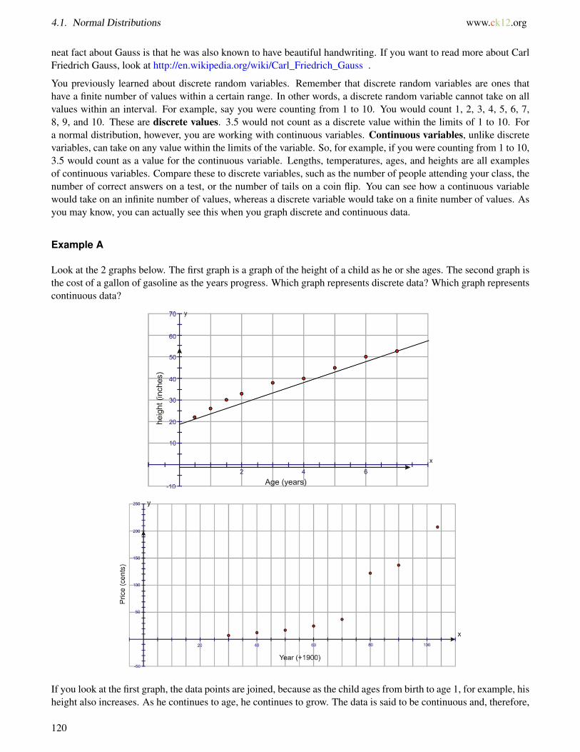
Look at the 2 graphs below. The first graph is a graph of the height of a child as he or she ages. The second graph isthe cost of a gallon of gasoline as the years progress. Which graph represents discrete data? Which graph representscontinuous data?

If you look at the first graph, the data points are joined, because as the child ages from birth to age 1, for example, hisheight also increases. As he continues to age, he continues to grow. The data is said to be continuous and, therefore,

120

www.ck12.org Chapter 4. Probability Distributions

you can connect the points on the graph. For the second graph, the price of a gallon of gas at the end of each yearis recorded. In 1930, a gallon of gas cost 10�c. You would not have gone in and paid 10.2�c or 9.75�c. The data is,therefore, discrete, and the data points cannot be connected.

Let’s look at a few problems to show how histograms approximate normal distribution curves.

Example B

Jillian takes a survey of the heights of all of the students in her high school. There are 50 students in her school. Sheprepares a histogram of her results. Is the data normally distributed?

If you take a normal distribution curve and place it over Jillian’s histogram, you can see that her data does notrepresent a normal distribution.

If the histogram were actually shaped like a normal distribution, it would have a shape like the curve below:

Example C

Thomas did a survey similar to Jillian’s in his school. His high school had 100 students. Is his data normallydistributed?

121

4.1. Normal Distributions www.ck12.org

If you take a normal distribution curve and place it over Thomas’s histogram, you can see that his data also does notrepresent a normal distribution.

Guided Practice

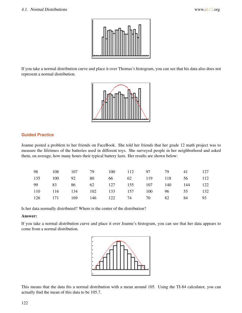
Joanne posted a problem to her friends on FaceBook. She told her friends that her grade 12 math project was tomeasure the lifetimes of the batteries used in different toys. She surveyed people in her neighborhood and askedthem, on average, how many hours their typical battery lasts. Her results are shown below:

98 108 107 79 100 112 97 79 41 127

135 100 92 80 66 62 119 118 56 112

99 83 86 62 127 155 107 140 144 122

110 116 134 102 133 157 100 96 55 132

126 171 169 146 122 74 70 82 84 93

Is her data normally distributed? Where is the center of the distribution?

Answer:

If you take a normal distribution curve and place it over Joanne’s histogram, you can see that her data appears tocome from a normal distribution.

This means that the data fits a normal distribution with a mean around 105. Using the TI-84 calculator, you canactually find the mean of this data to be 105.7.

122

www.ck12.org Chapter 4. Probability Distributions

What Joanne’s data does tell us is that the mean score (105.7) is at the center of the distribution, and the data fromall of the other scores (times) are spread from that mean. You will be learning much more about standard normaldistributions in a later Concept. But for now, remember the 2 key points about a standard normal distribution. Thefirst key point is that the data represented is continuous. The second key point is that the data is centered at the meanand is symmetrically distributed on either side of that mean.

Practice

1. The following data was collected on a recent 25-point math quiz. Does the data represent a normal distribu-tion? Can you determine anything from the data?

20 17 22 23 25

14 15 14 17 9

18 2 11 18 19

14 21 19 20 18

16 13 14 10 12

2. A recent blockbuster movie was rated PG, with an additional violence warning. The manager of a movietheater did a survey of moviegoers to see what ages were attending the movie in an attempt to see if peoplewere adhering to the warnings. Is his data normally distributed? Do moviegoers at the theater regularly adhereto warnings?

17 9 20 27 16

15 14 24 19 14

19 7 21 18 12

5 10 15 23 14

17 13 13 12 14

3. The heights of coniferous trees were measured in a local park in a regular inspection. Is the data normallydistributed? Are there areas of the park that seem to be in danger? The measurements are all in feet.

123

4.1. Normal Distributions www.ck12.org

22.8 9.7 23.2 21.2 23.5

18.2 7.0 8.8 25.7 19.4

25.0 8.8 23.0 23.2 20.1

23.1 18.5 21.7 21.7 9.1

4.3 7.8 3.4 20.0 8.5

Determine if the points representing each of the following data sets can be connected when graphed.

4. The number of students enrolled in a college each semester5. The weight of a baby seal each day as it grows6. The number of coins a coin collector owns each week7. The speed of a rocket each second as it accelerates8. The amount of water in a swimming pool each minute as it is drained9. The number of employees a company has each month as it expands

10. The thickness of a glacier each year as it melts

124