416678_731334298_773159429

8/6/2019 416678_731334298_773159429

http://slidepdf.com/reader/full/416678731334298773159429 1/16

PLEASE SCROLL DOWN FOR ARTICLE

This article was downloaded by: [University of Tokyo]

On: 14 February 2011

Access details: Access Details: [subscription number 932576267]

Publisher Taylor & Francis

Informa Ltd Registered in England and Wales Registered Number: 1072954 Registered office: Mortimer House, 37-

41 Mortimer Street, London W1T 3JH, UK

Vehicle System DynamicsPublication details, including instructions for authors and subscription information:http://www.informaworld.com/smpp/title~content=t713659010

Cornering stiffness estimation based on vehicle lateral dynamicsC. Sierraa; E. Tsengb; A. Jaina; H. Penga

a Department of Mechanical Engineering, University of Michigan, Ann Arbor, Michigan, USA b

Research/Advanced Engineering, Ford Motor Company,

To cite this Article Sierra, C. , Tseng, E. , Jain, A. and Peng, H.(2006) 'Cornering stiffness estimation based on vehiclelateral dynamics', Vehicle System Dynamics, 44: 1, 24 — 38

To link to this Article: DOI: 10.1080/00423110600867259

URL: http://dx.doi.org/10.1080/00423110600867259

Full terms and conditions of use: http://www.informaworld.com/terms-and-conditions-of-access.pdf

This article may be used for research, teaching and private study purposes. Any substantial orsystematic reproduction, re-distribution, re-selling, loan or sub-licensing, systematic supply ordistribution in any form to anyone is expressly forbidden.

The publisher does not give any warranty express or implied or make any representation that the contentswill be complete or accurate or up to date. The accuracy of any instructions, formulae and drug dosesshould be independently verified with primary sources. The publisher shall not be liable for any loss,actions, claims, proceedings, demand or costs or damages whatsoever or howsoever caused arising directlyor indirectly in connection with or arising out of the use of this material.

http://www.informaworld.com/smpp/title~content=t713659010

http://dx.doi.org/10.1080/00423110600867259

http://www.informaworld.com/terms-and-conditions-of-access.pdf

http://www.informaworld.com/terms-and-conditions-of-access.pdf

http://dx.doi.org/10.1080/00423110600867259

http://www.informaworld.com/smpp/title~content=t713659010

8/6/2019 416678_731334298_773159429


Vehicle System Dynamics

Vol. 44, Supplement, 2006, 24–38

Cornering stiffness estimation based on vehicle

lateral dynamics

C. SIERRA†, E. TSENG‡, A. JAIN† and H. PENG*†

†Department of Mechanical Engineering, University of Michigan, Ann Arbor, Michigan, USA‡Research/Advanced Engineering, Ford Motor Company

In this article, the cornering stiffness estimation problem based on the vehicle bicycle (one-track)model is studied. Both time-domain and frequency-domain-based methods are analyzed, aiming toestimate the effective cornering stiffness, defined as the ratio between the lateral force and the slipangle at the two axles. Several methods based on the bicycle model were developed, each havingspecific pros/cons related to practical implementations. The developed algorithms were evaluated onthe basis of the simulation data from the bicycle model and the CarSim TM software. Finally, selectedalgorithms were evaluated using experimental data.

Keywords: Road friction estimation; Tire force; Lateral dynamics

1. Introduction

Tire/road friction is an important characteristic that influences vehicle longitudinal,

lateral/yaw and roll motions. The tire/road friction coefficient, if accurately and timely

obtained, could significantly impact the design and performance of active safety systems.

This is because vehicle motions are predominantly affected through the tire forces, governed

by road friction and tire normal forces. In the literature, the majority of tire–road friction

estimation schemes use features of tire/tread behavior (e.g. wheel speed, wheel acceleration,

aligning moment, tire noise) as the basis of the estimation. For example, Eichhorn and Roth [1]

used optical and noise sensors at the front-end of the tire, and stress and strain sensors inside the

tire’s tread to study both parameter-based and effect-based road friction estimation methods.Ito et al. [2] used the applied traction force and the resulting wheel speed difference between

driven and non-driven wheels to estimate the road surface condition. Pal et al. [3] applied

the neural-network-based identification technique to predict the road frictional coefficient

based on steady-state vehicle response signals. Pasterkamp [4] developed an on-line estima-

tion method based on lateral force and self-aligning torque measurements and the Delft tyre

model. Gustafsson [5] developed a model-based approach, and used the difference between

driven and un-driven wheels to detect the tire–road friction. Liu and Peng [6] applied the

special structure of the brush tire model and used the wheel speed signal to estimate the

*Corresponding author. Email: [email protected]

Vehicle System DynamicsISSN 0042-3114 print/ISSN 1744-5159 online © 2006 Taylor & Francis

http://www.tandf.co.uk / journalsDOI: 10.1080/00423110600867259

8/6/2019 416678_731334298_773159429


Cornering stiffness estimation 25

road friction coefficient and cornering stiffness. These friction estimation methods identify

tire/road characteristics by using longitudinal and tire dynamics, which can then be used for

the adaptations of control/estimation algorithm for both lateral and longitudinal directions.

The goal of this article is to study the possibility of using vehicle lateral/yaw dynamics

for the estimation of road friction, that is, based on the simple bicycle model (which is also

known as the one-track model). The assumption is that estimation methods using vehicle

motion data are fundamentally more robust when compared with those using tire behaviors.

The reason is that the tire has smaller inertia, and its behavior is influenced by road rough-

ness, anti-lock braking system (ABS) operation, tire pressure and tread variations, carcass

radial non-uniformities and vehicle roll/pitch/vertical motions. Therefore, tire motions tend

to be a lot more oscillatory and contain higher frequency components. Separating the effects

of these disturbances from those of tire/road friction is difficult. Another benefit of using

lateral/yaw dynamics for cornering stiffness estimation is that the related signals (such as

steering angle, yaw rate, lateral acceleration and vehicle forward speed) are readily measured

for other purposes. Therefore, incremental hardware cost is low.Estimation methods based on vehicle lateral/yaw dynamic equations (mostly based on the

bicycle model) can be divided into two categories: time-domain methods [7, 8] and transfer-

function methods [9]. The time-domain methods use the dynamic equations either directly or

in various combinational forms, and the underlying equations are correct even when the vehicle

is time-varying, for example, due to the variation of vehicle longitudinal speed or road friction.

On the other hand, the transfer-function representations of dynamic systems are accurate only

when the vehicle is time-invariant, and the effects of transient dynamics are ignored. Therefore,

transfer-function methods perform satisfactorily only under linear operating region where

cornering stiffness remains constant. In reference [9], both the transfer-function based method

and the variation-characteristic-speed-based method were presented. The latter can be said tobe a special case of transfer-function methods, as it uses the zero-frequency (steady-cornering)

information of the transfer function.

Despite of the benefits mentioned earlier, there are also drawbacks of using lateral/yaw

dynamics. As the frequency content of relevant signals is lower, the obtained estimation may

not be fast enough for certain applications, for example, ABS. In addition, vehicle lateral/yaw

dynamics are inherently low-pass, and thus the estimation results are not as sensitive as tire-

motion-based methods.

2. Vehicle model

The basis of our estimation methods is the bicycle (one-track) vehicle model, which describes

the vehicle lateral and yaw dynamics of a 2-axle, 1-rigid body ground vehicle (figure 1). The

state-space representation of this model is in the form

v

r

=

⎡⎢⎢⎣−(Cαf + Cαr)

mu

bC αr − aC αf

mu− u

bC αr − aC αf

I zzu

−(a2Cαf + b2Cαr)

I zzu

⎤⎥⎥⎦

v

r

+

⎡⎢⎢⎣

Cαf

maC αf

I zz

⎤⎥⎥⎦ δf (1)

where u is the vehicle forward speed, v the vehicle lateral speed, r the yaw rate, m the vehicle

mass, I zz the yaw moment of inertia, Cαf and Cαr are the front and rear cornering stiffness (per

axle), δf the front wheel steering angle, and a and b are the distances from the vehicle center

of gravity to front and rear axles, respectively.

8/6/2019 416678_731334298_773159429


26 C. Sierra et al.

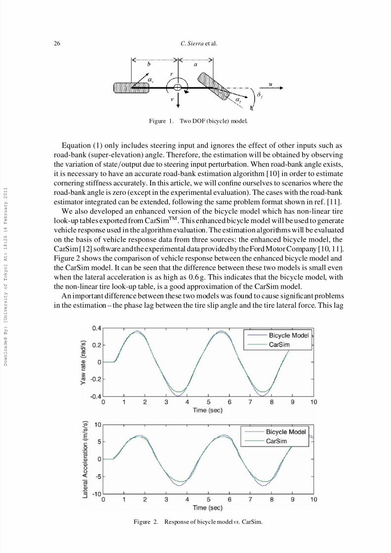
Figure 1. Two DOF (bicycle) model.

Equation (1) only includes steering input and ignores the effect of other inputs such as

road-bank (super-elevation) angle. Therefore, the estimation will be obtained by observing

the variation of state/output due to steering input perturbation. When road-bank angle exists,

it is necessary to have an accurate road-bank estimation algorithm [10] in order to estimate

cornering stiffness accurately. In this article, we will confine ourselves to scenarios where the

road-bank angle is zero (except in the experimental evaluation). The cases with the road-bank estimator integrated can be extended, following the same problem format shown in ref. [11].

We also developed an enhanced version of the bicycle model which has non-linear tire

look-up tables exported from CarSimTM. This enhanced bicycle model will be used to generate

vehicle response used in the algorithm evaluation. The estimation algorithms will be evaluated

on the basis of vehicle response data from three sources: the enhanced bicycle model, the

CarSim [12] software andthe experimental data provided by the Ford Motor Company [10, 11].

Figure 2 shows the comparison of vehicle response between the enhanced bicycle model and

the CarSim model. It can be seen that the difference between these two models is small even

when the lateral acceleration is as high as 0.6 g. This indicates that the bicycle model, with

the non-linear tire look-up table, is a good approximation of the CarSim model.

An important difference between these two models was found to cause significant problems

in the estimation – the phase lag between the tire slip angle and the tire lateral force. This lag

Figure 2. Response of bicycle model vs. CarSim.

8/6/2019 416678_731334298_773159429



Figure 3. Tire force vs. tire slip angle (CarSim simulation results).

is likely the result of the tire relaxation length included in the CarSim software as well as

the combination of the two (left and right) tire slip angles into one. The phase lag (shown

in figure 3) makes it somewhat difficult to define the ‘true cornering stiffness’ from CarSimsimulation results. As the stiffness to be estimated is the effective cornering stiffness, that is,

the tire lateral force over tire slip angle, there is a singular point in generating the reference

value when the tire slip angle passes through zero. Although the reference value differs from

the constant cornering stiffness we are accustomed to, in a linear tire model, the effective

cornering stiffness reflects the combined (left and right) lateral tire forces.

3. Direct method

This estimation method uses the two equations that form the state space of the bicycle vehiclemodel shown in equation (1). It is assumed that the vehicle parameters m, I zz, a and b and the

real-time measurements for δf , u , v and r are all available. We can use Euler’s approximation

or other filtering schemes to approximate the derivative, r (the lateral speed derivative). v,

if needed, is obtained in a different manner, as explained subsequently. Having all these

variables, we can algebraically solve the two equations (equations (2) and (3)) for Cαf and

Cαr. The rearranged form of the solution, as per the definition of the (effective) cornering

stiffness, is as follows

Cαf =(bvm + brmu+ I zzr)/L

(−v − ra+ δf u)/u=

F yf

αf

(2)

Cαr =(armu+ avm − I zzr)/L

(rb − v)/u=

F yr

αr

(3)

It should be noted that even though, in equations (2) and (3), it appears we are using the

derivative of the lateral velocity in the calculation, in the implementation, we actually use

8/6/2019 416678_731334298_773159429


28 C. Sierra et al.

ay − ur in place of v, which is much easier to measure when compared with v. It is important

to note that for this estimation method, the values for the cornering stiffness, Cαf and Cαr,

could approach infinity when the slip angles, αf and αr, approach zero during a transient

maneuver or when the vehicle is driving straight. Also, the slip angles could become large

as the longitudinal speed u approaches zero. Given that these two singularity conditions

create undesired estimation results, in the final implementation form, we will discard the

estimation of the cornering stiffness outside of a defined set of threshold limits and stop

the estimation scheme when the tire slip angle is small. In these cut-off cases, we will keep

the last estimated values as our best guess. This modification is necessary to ensure that the

overall estimation is reasonable. In addition, we will use signals within a horizon and use

the least-square solution to generate the best fit for the overall horizon. The direct method is

a straightforward two-unknown two-equation problem, and a reasonably good estimation is

usually obtained.

As stated before, the ‘direct method’ is conceptually simple and straightforward. The

problem is also numerically well-behaved. However, it requires both the lateral velocity (equiv-alently, side slip angle) and the derivative of the vehicle yaw rate – both of which are difficult

to obtain reliably in real applications. We will investigate its performance with the estimated

lateral velocity [11, 13], with simulation and experimental data. As this article is confined in

the analysis without the road-bank angle, the lateral velocity estimator will assume no bank.

In the next several sections, we will present several variations of the direct method, each

with its own benefits/drawbacks.

3.1 The ‘ay-method’

The basic idea of the so-called ‘ay -method’ is to eliminate reliance on the derivative of vehicleyaw rate. This can be achieved by using only the first equation (ay ) of the state-space equation

F y = may = Cαf αf + Cαrαr = Cαf

δ −

v + ar

u

+ Cαr

−

v − br

u

(4)

which can be rewritten in standard regression form

δ −

v + ar

u−

v − ar

u

Cαf

Cαr

= may (5)

Equation (5) can be formulated as a least-square estimation problem with one equation

and two unknowns. When signals at multiple sampling instances are used, the problem can

become over-determinate and the least-square solution can be obtained.The estimationmethod

includes the following drawbacks: it still requires lateral velocity (side slip angle) and it is an

under-determinate problem in nature and thus requires persistent excitation to obtain accurate

results.

3.2 The ‘rdot-method’

One of the most important disturbance to equation (1) is the road-bank angle. The presenceof gravity component in the lateral direction changes the lateral dynamics, and thus both the

direct method (equation (1)) and the ay -method (equation (5)) are susceptible to the presence

of road-bank angle. If one relies on the second equation of equation (1), that is, the yaw

acceleration equation (or the rdot equation), the resulting algorithm will be more robust with

8/6/2019 416678_731334298_773159429



respect to the road super-elevation disturbance. The fundamental equation is

M zz = I zzr = aC αf αf − bC αrαr = aC αf

δ −

v + ar

u

− bC αr

−

v − br

u

(6)

which can be rewritten asa

δ −

v + ar

u

− b

−

v − ar

u

Cαf

Cαr

= I zzr (7)

It can be seen that equation (7) relies on both lateral speed and yaw derivative. In addition,

when the vehicle is cornering in steady state, the yaw acceleration is zero. Therefore, [0; 0]

would be a solution for equation (7). This observation predicts that the rdot-method, that is, the

least-square estimation method based on equation (7), will not perform well when the vehicle

is cornering at steady state. In addition, equation (7) is also under-determinate in nature and

thus will work well only when persistent excitation condition is satisfied.

3.3 The ‘beta-less method’

All the three estimation methods require vehicle lateral velocity (or side slip angle), which

is difficult to measure. In addition, the ay -method and the rdot-method are both under-

determinate. The method to be proposed here aims to address both issues. We first start from

the lateral equation

may = F yf + F yr = Cαf δf − β −ar

u+ Cαr −β +

br

u (8)

based on which the lateral velocity can be solved

β =1

Cαf + Cαr

Cαf

δf −

ar

u

+ Cαr

br

u

− may

(9)

Plug in equation (9) into the yaw equation

I zzr = aF yf − bF yr = aC αf

δf − β −

ar

u

− bC αr

−β +

br

u

, (10)

one obtains mLay L

δ −

Lr

u

X1

X2

= I zzr + mbay , (11)

where

X1 ≡Cαf

Cαf + Cαr

and X2 ≡Cαf Cαr

Cαf + Cαr

.

After the intermediate parameters X1 and X2 were found, the cornering stiffness can be

calculated from

Cαr =X2

X1

and Cαf =X1

1 − X1

Cαr. (12)

It can be seen that the two intermediate variables determine the ratio and the magnitude of

the two cornering stiffness, respectively. In the least-square estimation problem formulation,

one could put different weightings to the two variables, for example, more weights on X2 to

promote magnitude convergence.

8/6/2019 416678_731334298_773159429


30 C. Sierra et al.

Table 1. Drawbacks of the four methods presented in section 3.

Sensitive to

Relies on r Relies on v Under-determinate road-bank angle

Direct method (equation (1)) Yes Yes Yesay method (equation (5)) Yes Yes Yes

rdot method (equation (7)) Yes Yes Yes

Beta-less method (equation (11)) Yes Yes Yes

The beta-less method can also be derived by relating the front and rear tire forces. Again

starting from the lateral equation

may = F yf + F yr = Cαf αf + Cαrαr = XC αr

αr +

δ −

Lr

u

+ Cαrαr

= (X + 1)F yr + XC αr

δ −

Lr

u

, where X = Cαf /Cαr,

(13)

one obtains F yr

δ −

Lr

u

X

Cαf

= F yf (14)

Note that equation (14) can be verified in the same manner as equation (11), where the lateral

forces F yf and F yr are computed by using the measurements ay and r.

3.4 Discussion

None of the four methods presented in this section is perfect. They all have certain drawbacks,

as shown in table 1. The ‘under-determinate’ issue refers to the fact the estimation problem

has more unknowns than equations. Therefore, information from multiple sampling points

needs to be used, and the information has to be persistently exciting for the estimation results

to converge to the true values. The last column is shown in grey color because one of the

authors had developed a robust algorithm for the road-bank angle estimation in an earlier

publication [10]. So from our viewpoint, that problem is not a major issue.

It is worthwhile to mention that the ‘under-determinate’ problem of the three estimation

methods shown in sections 3.1–3.3 can be eliminated by assuming that the ratio betweenthe front and rear cornering stiffness is fixed (which has been used in ref. [9]). This way, the

number of unknown variable is reduced to one, and most numerical problems and requirements

(persistent excitation) will disappear. Under steady cornering, when an under-determinate

method experiences difficulty, this addition assumption provides a reasonable way to ensure

good estimation results. In the later part of this article, when the beta-less method is augmented

with this assumption, we will refer to it as the ‘beta-less plus’ method.

4. Transfer-function method

This estimation method uses the transfer function from δf to r , obtained from the bicycle

vehicle model previously described. Even though the method might work for the transfer

function from δf to v as well, we use only the δf to r transfer function because measuring yaw

rate is more feasible and accurate than lateral velocity. If we re-write the state-space equation

8/6/2019 416678_731334298_773159429



in a simpler form: v

r

=

a1 a3

a2 a4

v

r

+

b1

b2

δf , (15)

then it is straightforward to write the transfer function from steering to yaw rate as

H δf →r(s) =b2s + (a2b1 − a1b2)

s2 − (a1 + a4)s + (a1a4 − a2a3)=

n1s + n2

s2 + d 1s + d 2(16)

where

d 1 =Cαf + Cαr

mu+

a2Cαf + b2Cαr

I zu,

d 2 =(Cαf + Cαr)(a2Cαf + b2Cαr) − (bC αr − aC αf )[(bC αr − aC αf ) − mu2]

mI zu2,

n1 =aC αf

I zand n2 =

LC αf Cαr

mI zu.

This method uses the available parameters (m, I zz, a and b) and the measurements (δf , u and r)

to obtain a least-square fit for the transfer function in real time. Ideally, in order not to rely

on the derivative(s) of yaw rate, the estimation algorithm will be applied to the discrete-time

format. In other words, the continuous-time transfer function shown in equation (16) should

first be converted to its discrete-time counter-part, which can then be used to formulate an

optimal estimation problem, for example, least-square ARX model identification problem.

The identified ARX model, which best describes the vehicle yaw motion in the discrete-time

format, will then be converted into the continuous-time where best-guess parameters of thetransfer function for the yaw rate output [equation (16)] can be obtained. As the parameters of

the continuous time transfer function are related to the cornering stiffness, it results in a non-

linear set of four equations with two unknowns. We can solve this system using a least-square

approach to obtain the best guess for the cornering stiffness.

5. Simulation results

In this section, the performance of the five methods are studied using the simulation data taken

from the bicycle model with non-linear tires as well as the CarSim [12] software, for whichmodel the input was the steering wheel angle. The estimation schemes, however, assume that

the tire steering angle is directly measured. Therefore, the steering system dynamics included

in the CarSim software will not have any adverse effect on our estimation results. In sections 5.1

and 5.2, we will examine the results of the four time-domain-based algorithms. In section 5.3,

we will present the results from the transfer-function-based method.

5.1 Results based on the enhanced bicycle model data

We first examine the performance of the four time-domain estimation methods with the vehicle

response data generated from the enhanced bicycle model. In this case, there is almost no uncer-tainty. The only uncertainty, from the viewpoint of the estimation methods, is the difference

between the linear tire and the non-linear tire model. The results in this section serve to weed

out the weakest algorithms so that future study will be more focussed. In addition, to fully

demonstrate the performance of the algorithms in its cleanest form, we are not imposing any

8/6/2019 416678_731334298_773159429


32 C. Sierra et al.

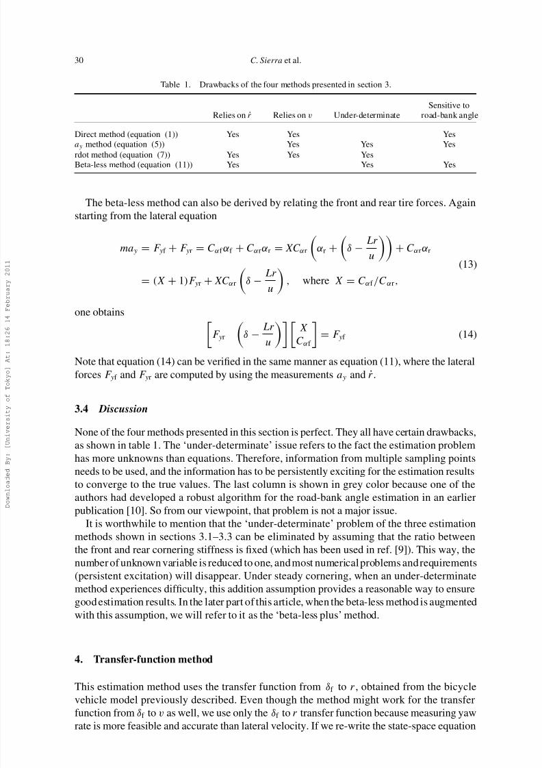
Figure 4. Estimation performance of the time-domain estimation methods (bicycle model data, J-turn).

Figure 5. Estimation performance of the time-domain estimation methods (bicycle model data, slalom test).

filtering/saturation of the estimation results. For example, the estimated cornering stiffness

values may become negative even though we know they should not. In all algorithms, the

vehicle input and output data are obtained at the rate of 100 Hz, and 10 data points (over a100 m s window) are used for the least-square estimations. Results from three maneuvers are

presented: constant cornering (J-turn), slalom and fish hook. The results are shown in figures 4,

5 and 6, respectively.

It can be seen that the performance of the ay -method and the rdot method is significantly

worse than the other two methods. For the direct method and the beta-less method, the perfor-

mance is quite satisfactory. Other than during the initial phase, when the estimated variables

converge gradually, both methods produce results that are very close to the true values all the

time. In the following sections, we will focus on the direct method and the beta-less method

for all future studies.

5.2 Results based on the CarSim data

In this section, the simulation data from the CarSim software is used. A major factor that

needs to be considered is the availability of lateral velocity, which is difficult to measure in

8/6/2019 416678_731334298_773159429



Figure 6. Estimation performance of the time-domain estimation methods (bicycle model data, fishhook).

the field. We will present results for two cases: when all needed signals are measured and

when the lateral speed is estimated by using the algorithm presented in ref. [13]. Figures 7 and

8 show the results under two maneuvers: sinusoidal and fish hook. In each figure, we show

the vehicle yaw rate and lateral velocity, which indicates the severity of the maneuver, and the

estimation results. In the sinusoidal maneuver, the beta-less method performs better than the

direct method – the latter exhibits some unwanted fluctuation due to zero crossing of the slip

angle. When the estimated lateral velocity is used, the direct method performance is improved

slightly.

In the fish hook maneuver, the direct method performs well, whereas the beta-less methoddoes not. This is because the fish hook maneuver is not persistently exciting. Under this

case, using the ‘plus-up trick’ (i.e., assuming Cαf /Cαr = 1.2) helps the beta-less method

significantly. However, it can be seen that the transient performance suffers slightly. Therefore,

Figure 7. Estimation performance of the time-domain estimation methods (CarSim data, sinusoidal).

8/6/2019 416678_731334298_773159429


34 C. Sierra et al.

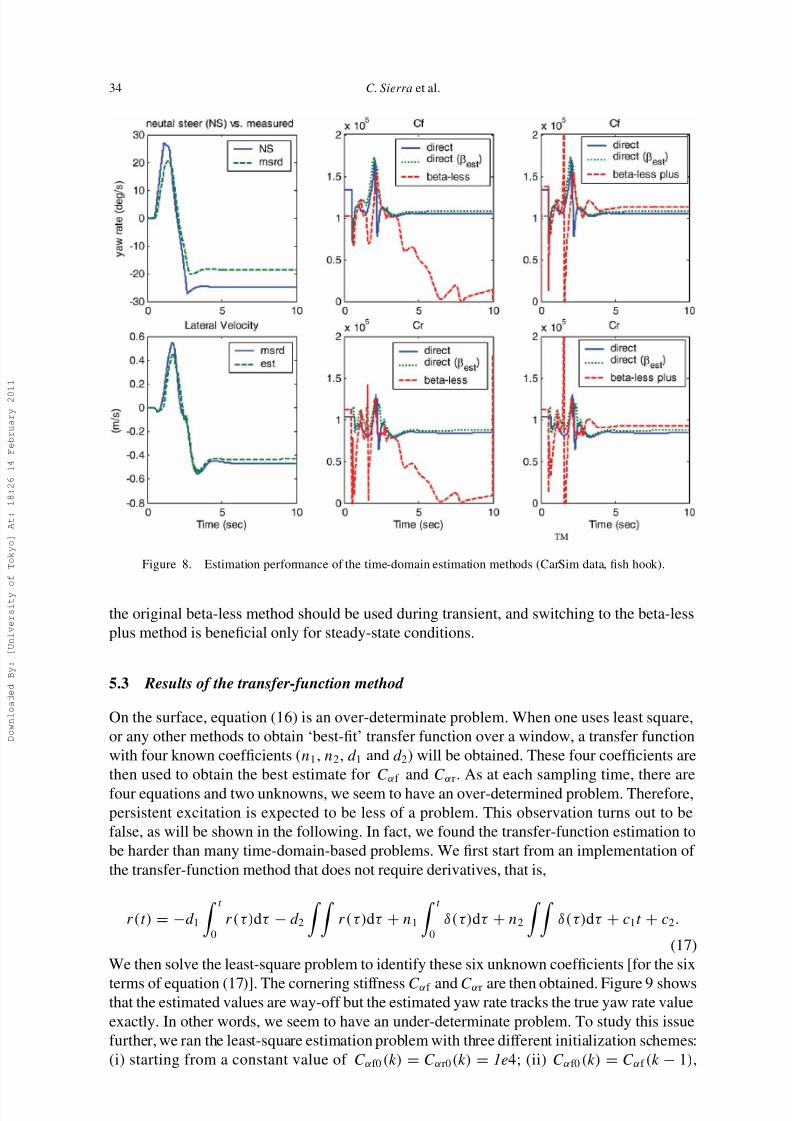
Figure 8. Estimation performance of the time-domain estimation methods (CarSim data, fish hook).

the original beta-less method should be used during transient, and switching to the beta-less

plus method is beneficial only for steady-state conditions.

5.3 Results of the transfer-function method

On the surface, equation (16) is an over-determinate problem. When one uses least square,

or any other methods to obtain ‘best-fit’ transfer function over a window, a transfer function

with four known coefficients (n1, n2, d 1 and d 2) will be obtained. These four coefficients are

then used to obtain the best estimate for Cαf and Cαr. As at each sampling time, there are

four equations and two unknowns, we seem to have an over-determined problem. Therefore,

persistent excitation is expected to be less of a problem. This observation turns out to be

false, as will be shown in the following. In fact, we found the transfer-function estimation to

be harder than many time-domain-based problems. We first start from an implementation of

the transfer-function method that does not require derivatives, that is,

r(t) = −d 1

t

0

r(τ)dτ − d 2

r(τ)dτ + n1

t

0

δ(τ)dτ + n2

δ(τ)dτ + c1t + c2.

(17)

We then solve the least-square problem to identify these six unknown coefficients [for the six

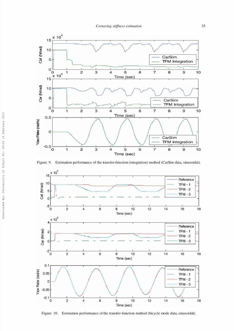
terms of equation (17)]. The cornering stiffness Cαf and Cαr are then obtained. Figure 9 showsthat the estimated values are way-off but the estimated yaw rate tracks the true yaw rate value

exactly. In other words, we seem to have an under-determinate problem. To study this issue

further, we ran the least-square estimation problem with three different initialization schemes:

(i) starting from a constant value of Cαf0 (k) = Cαr0 (k) = 1e4; (ii) Cαf0 (k) = Cαf (k − 1),

8/6/2019 416678_731334298_773159429



Figure 9. Estimation performance of the transfer-function (integration) method (CarSim data, sinusoidal).

Figure 10. Estimation performance of the transfer-function method (bicycle mode data, sinusoidal).

8/6/2019 416678_731334298_773159429


36 C. Sierra et al.

Cαr0 (k) = Cαr(k − 1); (iii) Cαf0 (k) = Cαf_true, Cαr0 (k) = Cαr_true. These three estimation

methods, referred as TFM1, TFM2 and TFM3, will be tested under an imaginary case when the

(original) bicycle model cornering stiffness is varying slowly. The estimation results are shown

in figure 10. All the three methods result in perfectly reconstructed yaw rate. However, the

cornering stiffness values are quite different – in other words, we have an under-determinate

problem. This fact makes it extremely difficult to obtain accurate cornering stiffness using

the transfer-function method. Using the original equation (16) (using derivatives of signals)

reduces the number of unknowns to 4, but the results are still unsatisfactory. We had also tried

a discrete-time implementation, but the results were similar.

6. Experimental results

In this section, the performance of the direct method and the beta-less methods is studied

using test data from a Lincoln Mark 8 vehicle, obtained at the Smithers Winter Test Center(low friction) and Ford Michigan Proving Ground (high friction) [10, 11]. The steering inputs

and the vehicle speed were controlled by a human driver and vary in an arbitrary fashion. All

vehicle lateral dynamical variables are directly measured, except lateral speed, which may be

measured or estimated [13]. All the test data were measured at the sampling time of 7 m s.

Two challenging test conditions were selected: slalom on a high-mu and banked road surface

and wobbly on icy surface. In the first case (figure 11), the lateral speed estimation has an

Figure 11. Estimation performance of the direct and beta-less methods (test data, high-mu on bank).

8/6/2019 416678_731334298_773159429



Figure 12. Estimation performance of the direct and beta-less methods (test data, low-mu flat road).

obvious offset. Both versions of the direct methods return estimated values that are slightly

below the true value. The beta-less plus method, on the contrary, returns reasonable results.

It should be noted that in this severe slalom maneuver, the true effective cornering stiffness

should fluctuate somewhat similar to the case shown in figure 5. In the test, as we do not have

a real-time measurement of tire cornering stiffness, we are only showing the nominal high-mu

value which indicates where the true value should be roughly located.

In the icy-road scenario (figure 12), again there is no way we can measure the true values of

the cornering stiffness. The true value is lower than the ‘high-mu nominal’ line shown in the

plots, but we do not know exactly where. The estimated results of the two methods are quitedifferent, and we cannot tell for certain which method is more accurate. More experimental

work needs to be done, which the authors are inspired to work on.

7. Conclusions

In this article, we studied the application of vehicle lateral dynamic equations to the estimation

of tire cornering stiffness. The estimation methods are based on the simple bicycle model and

common lateral/yaw measurement. It was found that the under-determinateness is a majorissue and should be avoided if possible. Among all the methods studied, the direct method

and the beta-less method were found to have the highest potential for field implementation.

Preliminary study using pre-recorded experimental data shows that they work reasonably well

under two highly challenging experimental scenarios.

8/6/2019 416678_731334298_773159429


38 C. Sierra et al.

References

[1] Eichhorn, U. and Roth, J., 1992, Prediction and monitoring of tyre/road friction, Proceedings FISITA, London,June.

[2] Ito, M., Yoshioka, K. and Saji, T., 1994, Estimation of road surface conditions using wheel speed behavior. SAE

paper no. 9438826.[3] Pal, C., Hagiwara,I., Morishita, S. and Inoue, H., 1994,Application of neural networksin real time identificationof dynamic structural response and prediction of road-friction coefficient from steady state automobile response.SAE paper no. 9438817.

[4] Pasterkamp, W.R., 1997, The Tyre as Sensor to Estimate Friction (Delft, The Netherlands: Delft UniversityPress).

[5] Gustafsson, F., 1998, Monitoring tire–road friction using the wheel slip. IEEE Control Systems Magazine, 18,42–49.

[6] Liu, C. and Peng, H., 1996, Road friction coefficient estimation for vehicle path prediction. Vehicle System

Dynamics, 25(Suppl.), 413–425.[7] Han,J., Rajamani, R. andAlexander,L., 2002, GPS-based real-time identification of tire–road friction coefficient.

IEEE Transaction on Control System Technology, 10(3), 331–343.[8] Arndt, M., Ding, E.L. and Massel, T., 2004, Identification of cornering stiffness during lane change maneuvers.

Proceedings of the 2004 International Conference on Control Applications, Taipei, Taiwan, pp. 344–349.

[9] Börner, M. and Isermann, R., 2004, Adaptive one-track model for critical lateral driving situations. Proceedingsof the 6th International Symposium on Advanced Vehicle Control (AVEC), Hiroshima, Japan.

[10] Tseng, H.E., 2001, Dynamic estimation of road bank angle. Vehicle System Dynamics, 36(4–5), 307–328.[11] Ungoren, A.Y., Peng, H. and Tseng, H., 2004, A Study on lateral speed estimation methods. International

Journal of Vehicle Autonomous Systems, 2(1/2), 126–144.[12] Mechanical Simulation Corporation, Ann Arbor, MI 48103, http://www.carsim.com/[13] Tseng, H.E., 2002, A sliding mode lateral velocity observer. Proceedings of the 6th International Symposium

on Advanced Vehicle Control (AVEC), Hiroshima, Japan.

416678_731334298_773159429

Documents

Transcript of 416678_731334298_773159429