4. Stability Analysis for Non-linear Ordinary Differential ...ggeorge/9420/notes/H4.pdf · ENGI...
78
ENGI 9420 Lecture Notes 4 - Stability Analysis Page 4.01 4. Stability Analysis for Non-linear Ordinary Differential Equations A pair of simultaneous first order homogeneous linear ordinary differential equations for two functions x(t), y(t) of one independent variable t, dx x ax by dt dy y cx dy dt = = + = = + may be represented by the matrix equation x a b x y c d y = A single second order linear homogeneous ordinary differential equation for x(t) with constant coefficients, 2 2 0 dx dx p qx dt dt + + = may be re-written as a linked pair of first order homogeneous ordinary differential equations, by introducing a second dependent variable: dx y dt dy qx py dt = =− − and may also be represented in matrix form 0 1 x x y q p y = − − The general solution for (x, y) in either case can be displayed graphically as a set of contour curves (or level curves) in a phase space. Sections in this chapter: 4.01 Motion of a Pendulum 4.02 Stability of Stationary Points 4.03 Linear Approximation to a System of Non-Linear ODEs (1) 4.04 Reminder of Linear Ordinary Differential Equations 4.05 Stability Analysis for a Linear System 4.06 Linear Approximation to a System of Non-Linear ODEs (2) 4.07 Limit Cycles 4.08 Van der Pol’s Equation 4.09 Theorem for Limit Cycles 4.10 Lyapunov Functions [for reference only - not examinable] 4.11 Duffing’s Equation 4.12 More Examples 4.13 Liénard’s Theorem
Transcript of 4. Stability Analysis for Non-linear Ordinary Differential ...ggeorge/9420/notes/H4.pdf · ENGI...

ENGI 9420 Lecture Notes 4 - Stability Analysis Page 4.01
4. Stability Analysis for Non-linear Ordinary Differential Equations A pair of simultaneous first order homogeneous linear ordinary differential equations for two functions x(t), y(t) of one independent variable t,
dxx ax b ydtdyy cx d ydt
= = +
= = +
may be represented by the matrix equation x a b xy c d y
=
A single second order linear homogeneous ordinary differential equation for x(t) with constant coefficients,
2
2 0d x dxp qxdt dt
+ + =
may be re-written as a linked pair of first order homogeneous ordinary differential equations, by introducing a second dependent variable:
dx ydtdy qx p ydt
=
= − −
and may also be represented in matrix form 0 1x x
y q p y
= − −
The general solution for (x, y) in either case can be displayed graphically as a set of contour curves (or level curves) in a phase space. Sections in this chapter: 4.01 Motion of a Pendulum 4.02 Stability of Stationary Points 4.03 Linear Approximation to a System of Non-Linear ODEs (1) 4.04 Reminder of Linear Ordinary Differential Equations 4.05 Stability Analysis for a Linear System 4.06 Linear Approximation to a System of Non-Linear ODEs (2) 4.07 Limit Cycles 4.08 Van der Pol’s Equation 4.09 Theorem for Limit Cycles 4.10 Lyapunov Functions [for reference only - not examinable] 4.11 Duffing’s Equation 4.12 More Examples 4.13 Liénard’s Theorem
ENGI 9420 4.01 - Pendulum Page 4.02
4.01 Motion of a Pendulum Consider a pendulum, moving under its own weight, without friction. The pendulum bob has mass m, the shaft has length L and negligible mass, and the angle of the shaft with the vertical is x. The tension along the shaft is T. The acceleration due to gravity is g (≈ 9.81 m s–2).
Resolving forces radially (centripetal force) Resolving forces transverse to the pendulum: ⇒ (1) The Maclaurin series expansion of sin x is: Provided the oscillations of the pendulum are small, (x << 1), sin x x≈ and the ordinary differential equation governing the motion of the pendulum is, to a good approximation, (2) (which is the ODE of simple harmonic motion)

ENGI 9420 4.01 - Pendulum Page 4.03
Let the angular velocity of the pendulum be d xv xdt
= = .
Then, using the chain rule of differentiation,
dvx vdt
= = =
The ODE (2) becomes (3) If at time t = 0 the pendulum is passing through its equilibrium position with angular speed vo, then the initial conditions are
( ) ( ) o0
0 0 , 0t
d xx v vdt =
= = =
Substituting the initial conditions into (2), (4) The x-v plane is called the phase plane.

ENGI 9420 4.01 - Pendulum Page 4.04
Returning to the more general case
2 2sin 0 , where gx k x kL
+ = = (1)
and again using
dv dv d x dvx v vdt d x dt d x
= = = ⋅ =
the ODE can be re-written as
2 2sin 0 sin 0dvv k x v dv k x dxdx
+ = ⇒ + =
(5) However, the kinetic energy is ( )21
2 m Lv . In the absence of friction, the sum of kinetic and potential energy is constant, so that the potential energy of the pendulum must be –mL2k2 cos x (= –mg L cos x , which makes sense upon examining the diagram on page 4.02). Each value of total energy 21
2E mL c= generates an orbit (or energy curve). The relationship between total energy and initial angular velocity is obtained from substituting the initial conditions (x = 0 and v = vo when t = 0) into (5):

ENGI 9420 4.01 - Pendulum Page 4.05
Recall that the angular velocity is just dxvdt
= .
Differentiating the complete solutions (6): 2 2 2 2o2 cos 2v k x v k− = − implicitly with
respect to time, we obtain This expression can also be derived directly from the ODE 2 sin 0x k x+ = (1).
When 0 < x < π and v > 0, 2
220 and sin 0dx d x dvv k x
dt dt dt= > = = − < .
Therefore, in the phase plane, as x increases from the starting point (0, vo), v decreases in the first quadrant, until the maximum value of x (label that maximum value of x as M).
Tracking back into the second quadrant, before (0, vo),
–π < x < 0 and v > 0 ⇒ 2
220 and sin 0dx d x dvv k x
dt dt dt= > = = − > .
The orbit increases from x = –M to a maximum at (0, vo), then decreases until x = +M. This tracks the motion of the pendulum on its complete swing from left to right. By symmetry, the swing in the opposite direction should generate a mirror image in the x axis of the phase plane, to complete the orbit.

ENGI 9420 4.01 - Pendulum Page 4.06
(6) ⇒ (7) Three cases arise: | vo | < 2k : In the first quadrant of the phase plane, the orbit will move right and down to an intercept
on the x axis at (M, 0), where osin and 02 2
vM Mk
π = + < <
. Extending to the
other three quadrants, the orbits resemble ellipses, centred on the origin. | vo | = 2k : The pendulum swings all the way to the upside-down position and comes to rest there, before either swinging back or continuing on in the same direction. | vo | > 2k : We can then generate the full set of orbits in the phase plane for the general pendulum problem.
ENGI 9420 4.01 - Pendulum Page 4.07
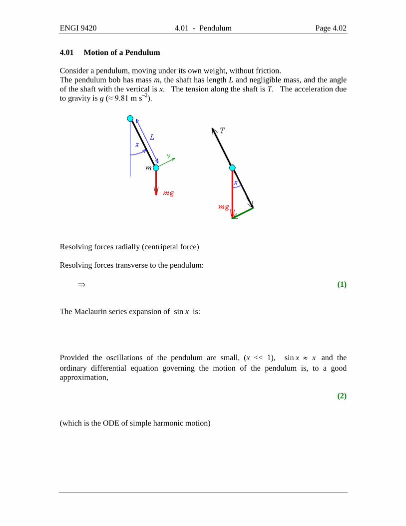
As time progresses, one moves along an orbit to the right above the x axis, but to the left
below the x axis
The relationship (7) between angular velocity v and angle x is itself a first order non-linear ordinary differential equation for x as a function of the time t:
2 222 2
o o2 sin 2 sin2 2
dx x dx xv k v kdt dt
= − ⇒ = ± −
2 2 2o 4 sin
2
dxt C
xv k⇒ ± = +
−
∫
For the case of closed orbits (| vo | < 2k), the time to complete one orbit (the period T of the pendulum) can be shown to be
o2 20
/24 , where sin and2 21 sin
vd M gT b kk k Lb
π θθ
= = = =−∫
This is a complete elliptic integral of the first kind, which has no analytic solution in terms of finite combinations of algebraic functions, (except for special choices of vo and k). As vo → 2k, the period T diverges to infinity – it takes forever for the zero energy pendulum to reach the upside-down position.
ENGI 9420 4.02 - Stability Page 4.08
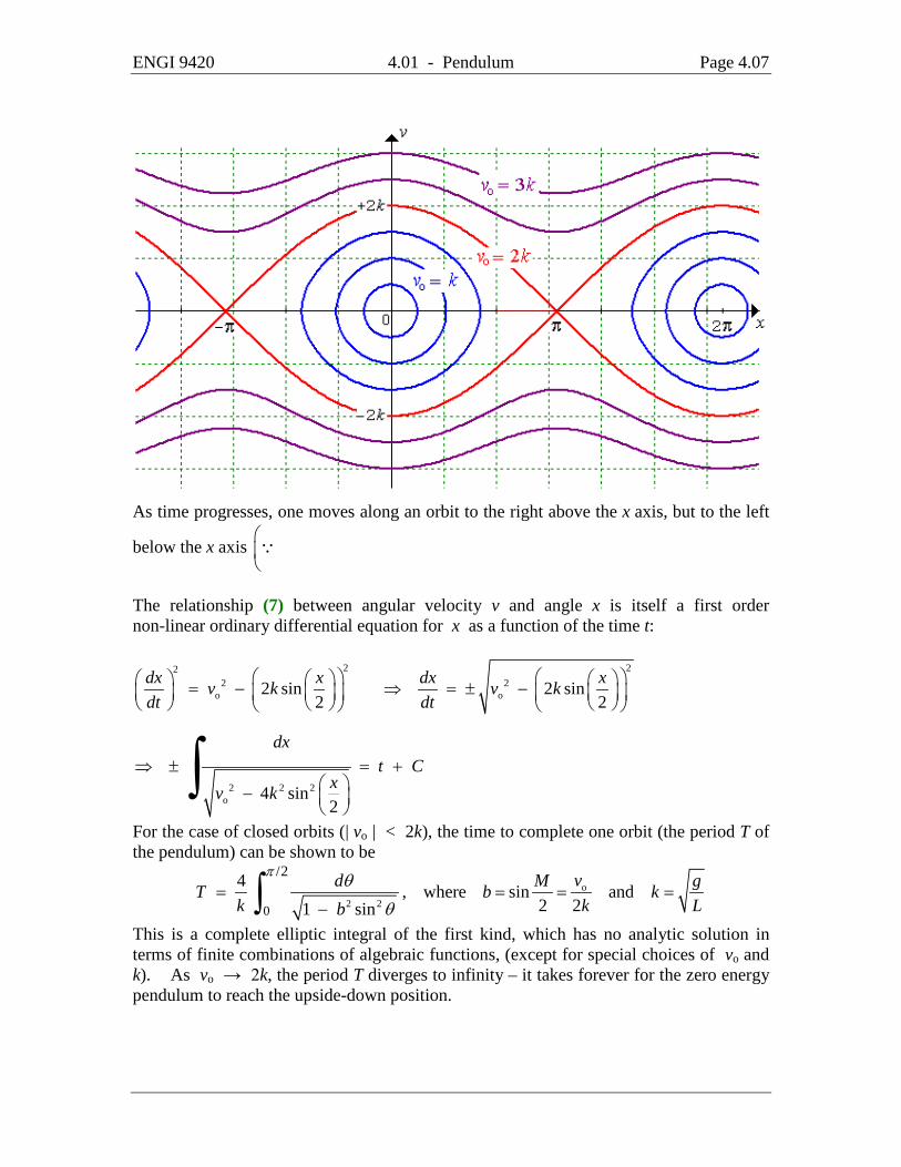
4.02 Stability of Stationary Points Consider the (generally non-linear) system of simultaneous first order ordinary differential equations
( ) ( ), , ,dx dyx P x y y Q x ydt dt
= = = = (1)
Using the chain rule, dydx
=
This can be integrated with respect to x to obtain a solution for y as an implicit function of x, provided P(x, y) ≠ 0. At points where P(x, y) = 0 but Q(x, y) ≠ 0, one may
integrate ( )( )
,,
P x ydxdy Q x y
= instead.
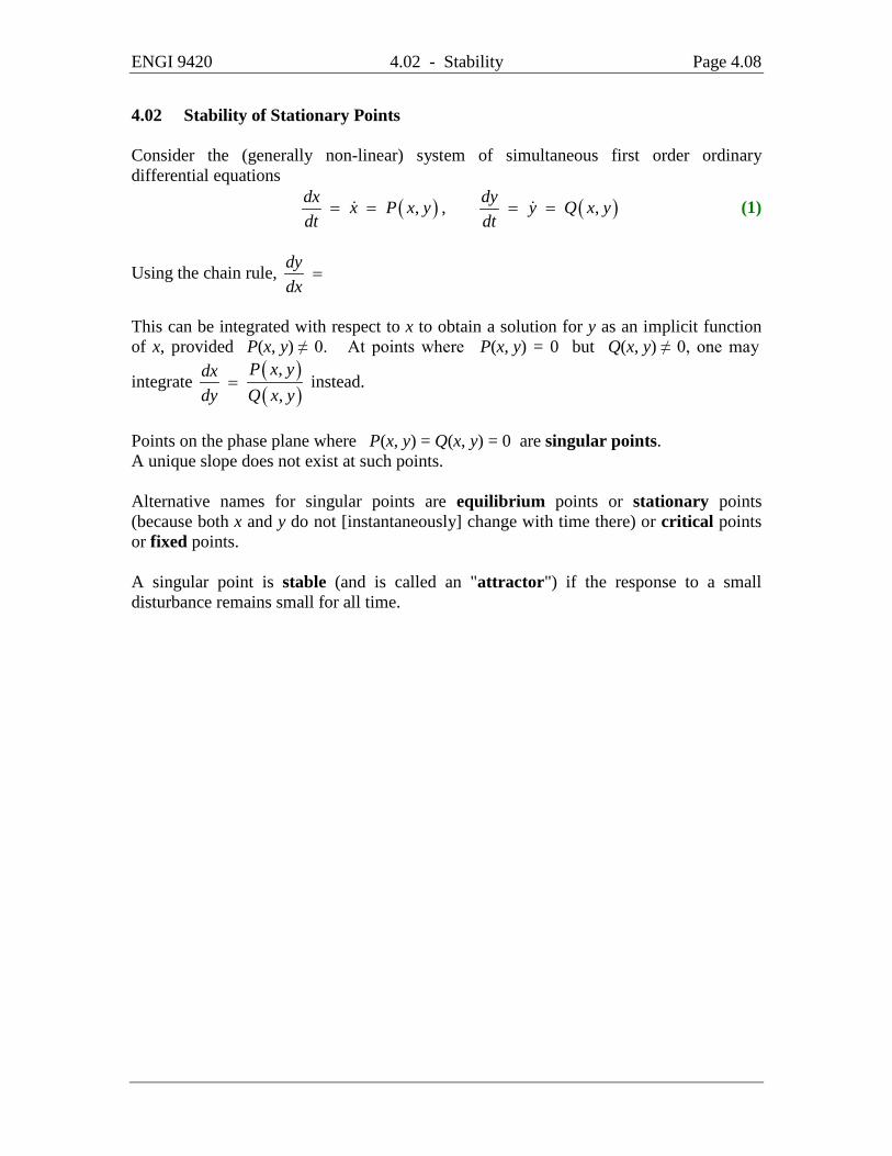
Points on the phase plane where P(x, y) = Q(x, y) = 0 are singular points. A unique slope does not exist at such points. Alternative names for singular points are equilibrium points or stationary points (because both x and y do not [instantaneously] change with time there) or critical points or fixed points. A singular point is stable (and is called an "attractor") if the response to a small disturbance remains small for all time.
ENGI 9420 4.02 - Stability Page 4.09
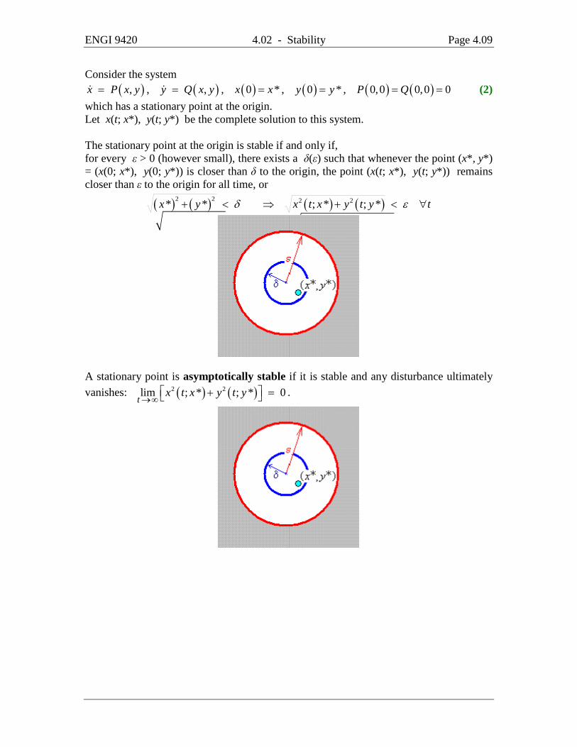
Consider the system ( ) ( ) ( ) ( ) ( ) ( ), , , , 0 * , 0 * , 0,0 0,0 0x P x y y Q x y x x y y P Q= = = = = = (2)
which has a stationary point at the origin. Let x(t; x*), y(t; y*) be the complete solution to this system. The stationary point at the origin is stable if and only if, for every ε > 0 (however small), there exists a δ(ε) such that whenever the point (x*, y*) = (x(0; x*), y(0; y*)) is closer than δ to the origin, the point (x(t; x*), y(t; y*)) remains closer than ε to the origin for all time, or
( ) ( ) ( ) ( )2 2 2 2* * ; * ; *x y x t x y t y tδ ε+ < ⇒ + < ∀
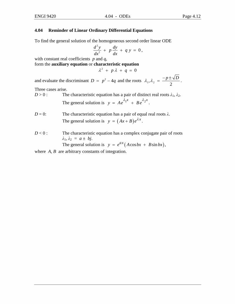
A stationary point is asymptotically stable if it is stable and any disturbance ultimately vanishes: ( ) ( )2 2lim ; * ; * 0
tx t x y t y
→∞ + = .

ENGI 9420 4.02 - Stability Page 4.10
Here are three types of stationary points with nearby orbits:

ENGI 9420 4.03 - Linear Approximation (1) Page 4.11
4.03 Linear Approximation to a System of Non-Linear ODEs (1) The Taylor series of any function f (x, y) about the point (x0, y0) is
( ) ( )( )
( )( )
( )
( )
( )( )
( ) ( )( )
( )0 0 0 0
0 0 0 0 0 0
0 0 0 0
2 22 2 20 0 0 0
2 2
, ,
, , ,
, ,
22! 2! 2!
x y x y
x y x y x y
f ff x y f x y x x y yx y
x x x x y y y yf f fx x y y
∂ ∂= + ⋅ − + ⋅ − +
∂ ∂
− − − −∂ ∂ ∂+ + +
∂ ∂ ∂ ∂
(1)
provided that the series converges to f (x, y). This allows us to create a linear approximation to the non-linear system
( ) ( ) ( ) ( ) ( ) ( ), , , , 0 * , 0 * , 0,0 0,0 0x P x y y Q x y x x y y P Q= = = = = = . (2)
( ) ( )( ) ( )
( )10,0 0,0
, 0,0 ,P PP x y P x y P x yx y
∂ ∂= + + +
∂ ∂ (3)
( ) ( )
( )1
2 2, 0,0
,where lim 0
x y
P x y
x y→=
+, (because P1(x, y) is at least second order in x, y)
and similarly for Q(x, y), so that the system becomes
( )( )
1
1
,
,
x ax b y P x y
y cx d y Q x y
= + +
= + +
(4)
where a, b, c, d are all constants. In the neighbourhood of the singular point (0, 0), this system can be modelled by the linear system
x ax b yy cx d y= += +
(5)
( ) ( ) ( ) ( )0,0 0,0 0,0 0,0
where , , , .P P Q Qa b c dx y x y
∂ ∂ ∂ ∂= = = =
∂ ∂ ∂ ∂
ENGI 9420 4.04 - ODEs Page 4.12
4.04 Reminder of Linear Ordinary Differential Equations To find the general solution of the homogeneous second order linear ODE
2
2 0d y dyp q ydx dx
+ + = ,
with constant real coefficients p and q, form the auxiliary equation or characteristic equation
2 0p qλ λ+ + =
and evaluate the discriminant 2 4D p q= − and the roots 1 2,2
p Dλ λ − ±= .
Three cases arise. D > 0 : The characteristic equation has a pair of distinct real roots λ1, λ2.
The general solution is 1 2x xy Ae B e
λ λ= + .
D = 0: The characteristic equation has a pair of equal real roots λ. The general solution is ( ) xy Ax B eλ= + . D < 0 : The characteristic equation has a complex conjugate pair of roots λ1, λ2 = a ± bj. The general solution is ( )cos sinaxy e A bx B bx= + , where A, B are arbitrary constants of integration.

ENGI 9420 4.04 - ODEs Page 4.13
To find the general solution of the system of simultaneous first order linear ODEs
dx ax b ydtdy cx d ydt
= +
= +
substitute the trial solution ( ) ( )( ) ( ), ,t tx t y t e eλ λα β= into the ODE, to obtain
or, in matrix form,
α = β = 0 is a solution (the trivial solution) for any choice of a, b, c, d and λ. Non-trivial solutions exist when the determinant of the matrix of coefficients is zero:
which is the characteristic equation of the system. The solutions to the characteristic equation are the eigenvalues of the coefficient matrix
a bA
c d
=
and, for each eigenvalue λ, a non-zero vectorαβ
that satisfies the equation
00
a bc dλ α
λ β−
= −
is an eigenvector for that eigenvalue. The general solution to the system of ODEs is a linear combination of the solutions arising from each eigenvalue:
( ) ( )( ) ( )1 1 2 2 1 1 2 21 2 1 2, ,t t t t
x t y t c e c e c e c eλ λ λ λ
α α β β= + +
unless the eigenvalues are equal, in which case the general solution is
( ) ( )( ) ( ) ( )( )1 1 2 2 1 1 2 2, ,t tx t y t c c t e c c t eλ λα α β β= + +
(where, in this case, (α1, β1) is not necessarily an eigenvector).

ENGI 9420 4.05 - Stability Analysis (Linear) Page 4.14
4.05 Stability Analysis for a Linear System In the case where (0, 0) is the only critical point of the system
dx ax b ydtdy cx d ydt
= +
= +
it follows that the characteristic equation ( ) ( )2 0a d ad bcλ λ− + + − = has only non-zero roots and that det 0A ad bc= − ≠ . Proof: If λ = 0 then at least one eigenvalue of the coefficient matrix A is zero, from which it follows immediately that
0det 0
0a b
A ad bcc d−
= = − =−
Both roots non-zero 0ad bc⇒ − ≠ . If (0, 0) is the only critical point of the system, then no other choice of (x, y) satisfies both equations
( )( )
0000
ad bc xax b yad bc ycx d y
− =+ =⇒
− =+ =
from which it follows immediately that det 0ad bc A− = ≠ . If the roots are both non-zero and (x, y) is a critical point of the system, then
( )( )
0000
ad bc xax b yad bc ycx d y
− =+ =⇒
− =+ =
But 1 2, 0 0ad bcλ λ ≠ ⇒ − ≠ ⇒ (0, 0) is the only solution to this pair of simultaneous linear equations. Therefore (0, 0) is the only critical point of the system if and only if both roots of the characteristic equation are non-zero.
ENGI 9420 4.05 - Stability Analysis (Linear) Page 4.15
Let ( ),i iα β be the eigenvector associated with the eigenvalue iλ of the coefficient matrix
a bA
c d
=
Let c1, c2 be arbitrary constants. Case of real, distinct, negative eigenvalues (with 2 1 0λ λ< < ): Two linearly independent solutions are
( ) ( )( ) ( ) ( ) ( )( ) ( )1 1 2 21 1 2 2, , and , ,t t t t
x t y t e e x t y t e eλ λ λ λ
α β α β= =
The general solution is
( ) ( )( ) ( )1 1 2 2 1 1 2 21 2 1 2, ,t t t t
x t y t c e c e c e c eλ λ λ λ
α α β β= + +
One can see that ( ) ( )( )lim ,t
x t y t→∞
=
If both arbitrary constants are zero, then we have the trivial solution (x = y = 0 for all t). If one of the arbitrary constants is zero (say c1), then
( ) ( )( ) ( ) ( )2 2 2 22 2, ,t t
x t y t c e c e y tλ λ
α β= ⇒ =
ENGI 9420 4.05 - Stability Analysis (Linear) Page 4.16
If neither arbitrary constant is zero, then
( )( )
( )
( )
( )
( )1 1 2 2 1 1 2 2 1 1 2 2
1 1 2 2 1 1 2 2 1 1 2 2
2 1 2 11 2
1 2 2 1 2 1
t tt t
t t t tc e c e c c e c e cy t
x t c e c e c c e c e c
λ λ λ λλ λ
λ λ λ λ λ λ
β β β β β β
α α α α α α
−
−
− −
− −
+ + += = =
+ + +
Because 2 1 0λ λ< < ,
( )( )
( )
( )1 1 2 2
1 1 2 2
2 1
2 1lim lim
t t
t
tc e cy t
x t c e c
λ λ
λ λ
β β
α α
−
−→−∞ →−∞
−
−
+= =
+
and
( )( )
( )
( )1 1 2 2
1 1 2 2
2 1
2 1lim limt t
t
tc c ey t
x t c c e
λ λ
λ λ
β β
α α→∞ →∞
−
−
+= =
+
All orbits therefore come in from infinity parallel to the line All orbits share the same tangent at the origin, We obtain a stable node that is also asymptotically stable. Case of real, distinct, positive eigenvalues (with 2 1 0λ λ> > ): The analysis leads to the same phase space, except that the arrows are reversed. The result is an unstable node.
ENGI 9420 4.05 - Stability Analysis (Linear) Page 4.17
Case of real, distinct eigenvalues of opposite sign (with 2 10λ λ< < ): The general solution is
( ) ( )( ) ( )1 1 2 2 1 1 2 21 2 1 2, ,t t t t
x t y t c e c e c e c eλ λ λ λ
α α β β= + +
( ) ( )( ) ( ) ( )( )2 10 lim , and lim ,t t
x t y t x t y tλ λ→−∞ →∞
< < ⇒
(with the exception of the orbit for c1 = 0). All orbits (except c1 = 0) therefore move away from the critical point at the origin. The system is unstable. If both arbitrary constants are zero, then we have the trivial solution (x = y = 0 for all t). If one of the arbitrary constants is zero (say c1), then
( ) ( )( ),x t y t =
If neither arbitrary constant is zero, then
( )( )
( )
( )
( )
( )1 1 2 2 1 1 2 2 1 1 2 2
1 1 2 2 1 1 2 2 1 1 2 2
2 1 2 11 2
1 2 2 1 2 1
t tt t
t t t tc e c e c c e c e cy t
x t c e c e c c e c e c
λ λ λ λλ λ
λ λ λ λ λ λ
β β β β β β
α α α α α α
−
−
− −
− −
+ + += = =
+ + +
Because 2 10λ λ< < ,
( )( )
( )
( )1 1 2 2
1 1 2 2
2 1
2 1lim lim
t t
t
tc e cy t
x t c e c
λ λ
λ λ
β β
α α
−
−→−∞ →−∞
−
−
+= =
+
and
( )( )
( )
( )1 1 2 2
1 1 2 2
2 1
2 1lim limt t
t
tc c ey t
x t c c e
λ λ
λ λ
β β
α α→∞ →∞
−
−
+= =
+

ENGI 9420 4.05 - Stability Analysis (Linear) Page 4.18
All orbits therefore share the same asymptotes,

ENGI 9420 4.05 - Stability Analysis (Linear) Page 4.19
Case of real, equal, negative eigenvalues ( 1 2 0λ λ= < ) and b = c = 0: The system is uncoupled:
dx axdtdy d ydt
=
=
and equal eigenvalues now require a = d = λ . The general solution is ( ) ( )( ) ( )1 2, ,t tx t y t c e c eλ λ= .
( ) ( )( ) ( ) ( )( )0 lim , and lim ,t t
x t y t x t y tλ→−∞ →∞
< ⇒ = = .
If both arbitrary constants are zero, then we have the trivial solution (x = y = 0 for all t). Additional Note: The eigenvalues of any triangular matrix are the diagonal entries of that matrix:
The characteristic equation of 0a b
Ad
=
is ( )det 0A Iλ− =
( )( ) 0 or0
a ba d a d
dλ
λ λ λλ
−⇒ = − − = ⇒ =
−
ENGI 9420 4.05 - Stability Analysis (Linear) Page 4.20
Case of real, equal, negative eigenvalues ( 1 2 0λ λ= < ) and b, c not both zero: The characteristic equation ( ) ( )2 0a d ad bcλ λ− + + − =
has the discriminant ( ) ( ) ( )2 24 4 0a d ad bc a d bc+ − − = − + = .
The solution of the characteristic equation simplifies to 2
a dλ += .
The general solution is ( ) ( )( ) ( ) ( )( )1 1 2 2 1 1 2 2, ,t tx t y t c c t e c c t eλ λα α β β= + + .
( ) ( )( ) ( ) ( ) ( )( ) ( )0 lim , , and lim , 0,0t t
x t y t x t y tλ→−∞ →∞
< ⇒ = ∞ ∞ = .
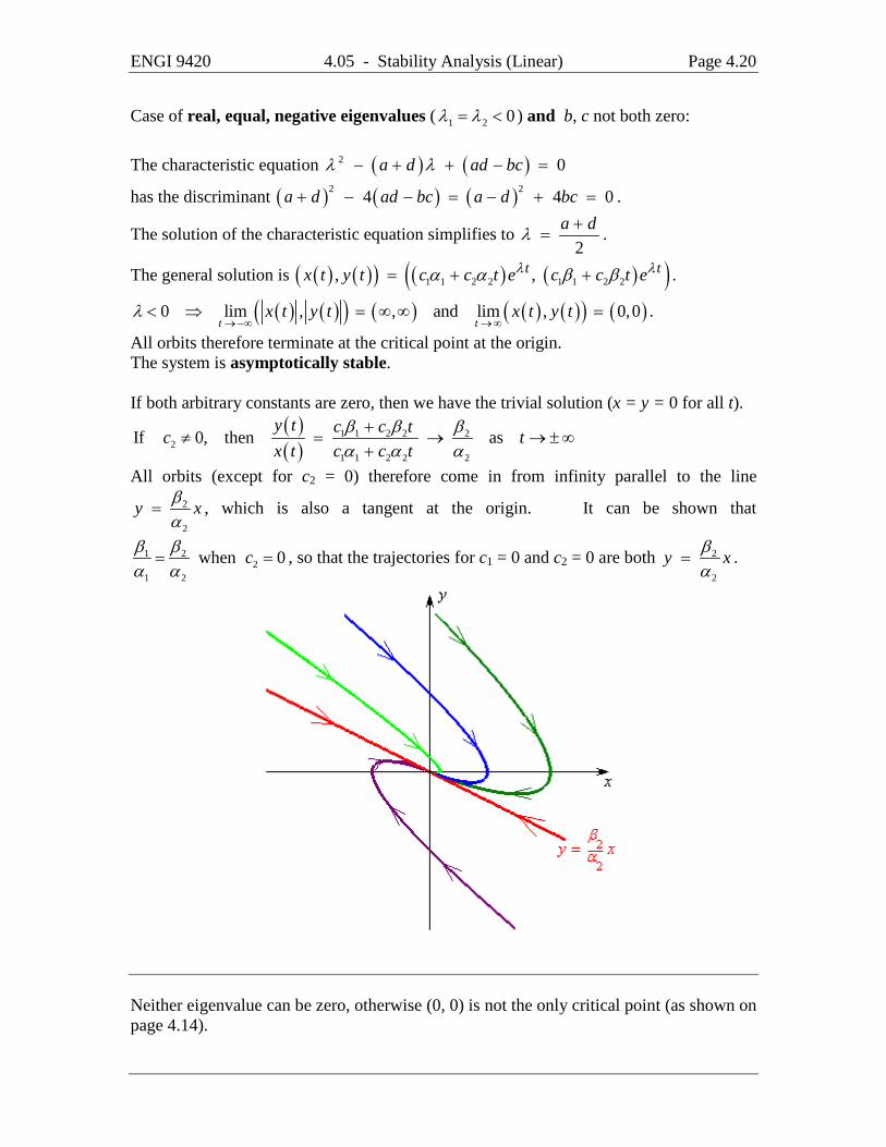
All orbits therefore terminate at the critical point at the origin. The system is asymptotically stable. If both arbitrary constants are zero, then we have the trivial solution (x = y = 0 for all t).
( )( )
1 1 2 2 22
1 1 2 2 2
If 0, then asy t c c tc tx t c c t
β β βα α α
+≠ = → → ±∞
+
All orbits (except for c2 = 0) therefore come in from infinity parallel to the line 2
2
y xβα
= , which is also a tangent at the origin. It can be shown that
1 22
1 2
when 0cβ βα α
= = , so that the trajectories for c1 = 0 and c2 = 0 are both 2
2
y xβα
= .
Neither eigenvalue can be zero, otherwise (0, 0) is not the only critical point (as shown on page 4.14).
ENGI 9420 4.05 - Stability Analysis (Linear) Page 4.21
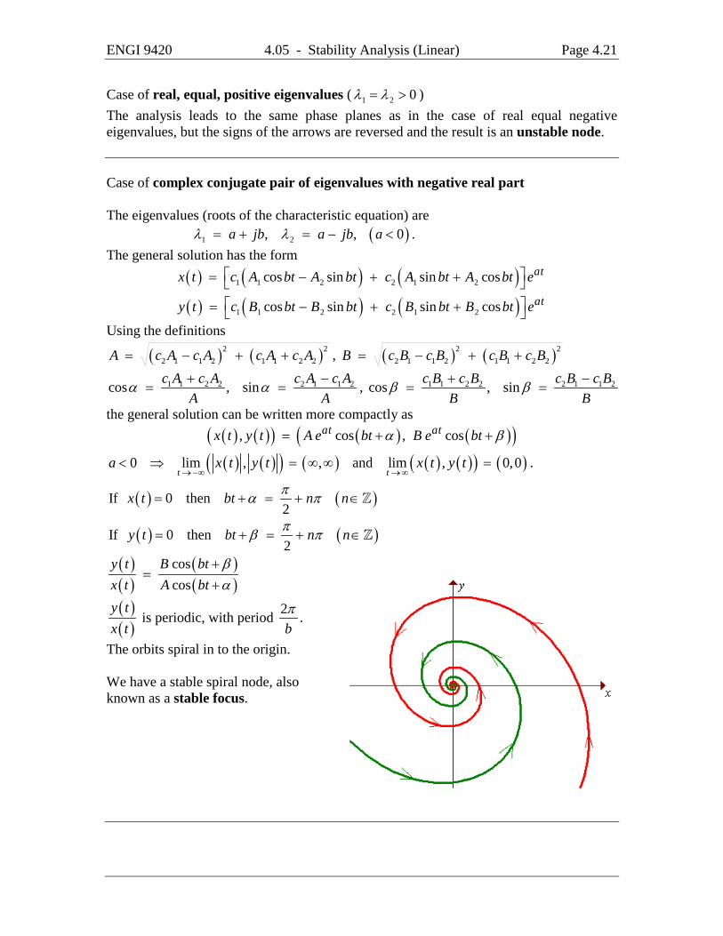
Case of real, equal, positive eigenvalues ( 1 2 0λ λ= > ) The analysis leads to the same phase planes as in the case of real equal negative eigenvalues, but the signs of the arrows are reversed and the result is an unstable node. Case of complex conjugate pair of eigenvalues with negative real part The eigenvalues (roots of the characteristic equation) are ( )1 2, , 0a jb a jb aλ λ= + = − < . The general solution has the form
( ) ( ) ( )( ) ( ) ( )
1 1 2 2 1 2
1 1 2 2 1 2
cos sin sin cos
cos sin sin cos
at
at
x t c A bt A bt c A bt A bt e
y t c B bt B bt c B bt B bt e
= − + + = − + +
Using the definitions
( ) ( )2 22 1 1 2 1 1 2 2A c A c A c A c A= − + + , ( ) ( )2 2
2 1 1 2 1 1 2 2B c B c B c B c B= − + +
1 1 2 2 2 1 1 2cos , sinc A c A c A c AA A
α α+ −= = , 1 1 2 2 2 1 1 2cos , sinc B c B c B c B
B Bβ β+ −
= =
the general solution can be written more compactly as ( ) ( )( ) ( ) ( )( ), cos , cosat atx t y t A e bt B e btα β= + +
( ) ( )( ) ( ) ( ) ( )( ) ( )0 lim , , and lim , 0,0t t
a x t y t x t y t→−∞ →∞
< ⇒ = ∞ ∞ = .
( ) ( )If 0 then2
x t bt n nπα π= + = + ∈
( ) ( )If 0 then2
y t bt n nπβ π= + = + ∈
( )( )
( )( )
coscos
y t B btx t A bt
βα
+=
+
( )( )
y tx t
is periodic, with period 2bπ .
The orbits spiral in to the origin. We have a stable spiral node, also known as a stable focus.

ENGI 9420 4.05 - Stability Analysis (Linear) Page 4.22
Case of complex conjugate pair of eigenvalues with positive real part The analysis leads to the same phase planes as in the case of negative real part, but the signs of the arrows are reversed and the result is an unstable focus. Case of complex conjugate pair of eigenvalues with zero real part (pure imaginary) The eigenvalues (roots of the characteristic equation) are 1 2,jb jbλ λ= − = + . The general solution has the compact form
( ) ( )( ) ( ) ( )( ), cos , cosx t y t A bt B btα β= + +
If 0 and2πα β= = − , then
ENGI 9420 4.05 - Stability Analysis (Linear) Page 4.23
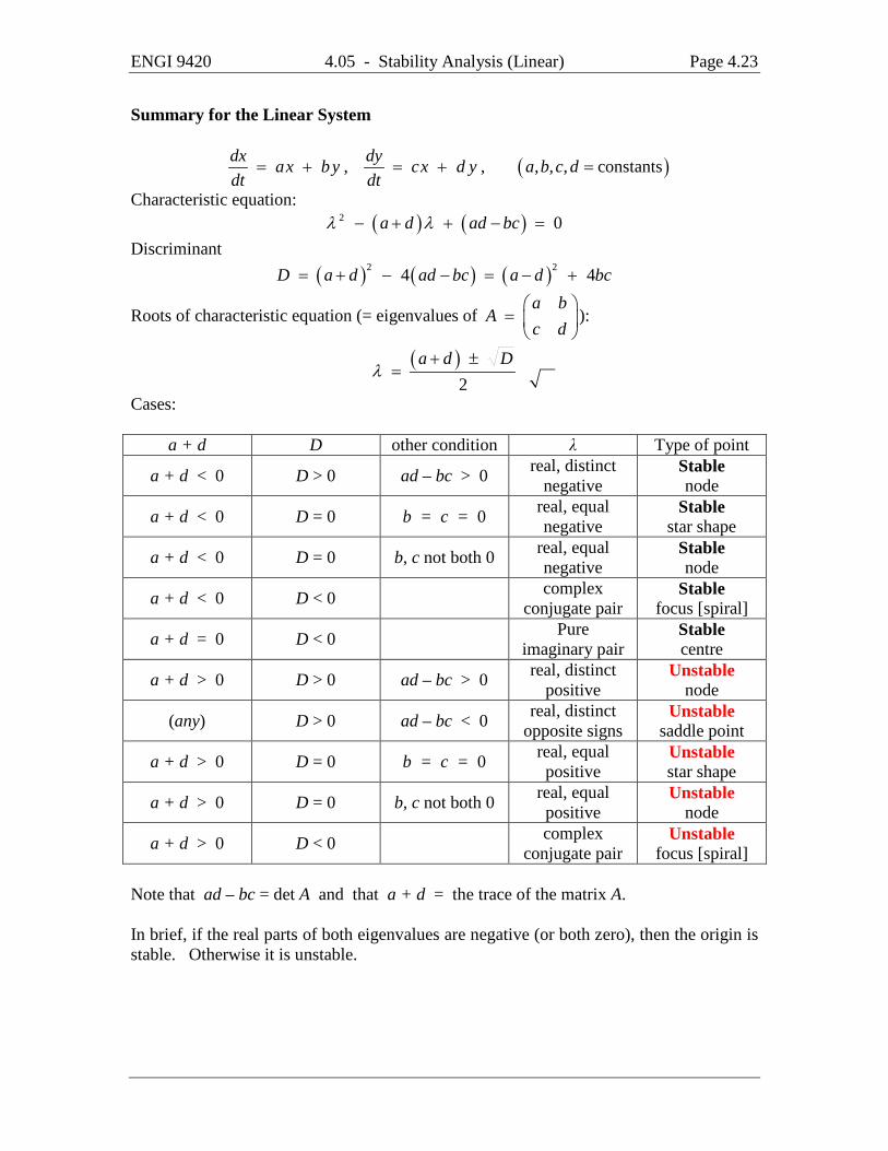
Summary for the Linear System
( ), , , , , constantsdx dyax b y cx d y a b c ddt dt
= + = + =
Characteristic equation: ( ) ( )2 0a d ad bcλ λ− + + − =
Discriminant ( ) ( ) ( )2 24 4D a d ad bc a d bc= + − − = − +
Roots of characteristic equation (= eigenvalues of a b
Ac d
=
):
( )2
a d Dλ
+ ±=
Cases:
a + d D other condition λ Type of point
a + d < 0 D > 0 ad – bc > 0 real, distinct negative
Stable node
a + d < 0 D = 0 b = c = 0 real, equal negative
Stable star shape
a + d < 0 D = 0 b, c not both 0 real, equal negative
Stable node
a + d < 0 D < 0 complex conjugate pair
Stable focus [spiral]
a + d = 0 D < 0 Pure imaginary pair
Stable centre
a + d > 0 D > 0 ad – bc > 0 real, distinct positive
Unstable node
(any) D > 0 ad – bc < 0 real, distinct opposite signs
Unstable saddle point
a + d > 0 D = 0 b = c = 0 real, equal positive
Unstable star shape
a + d > 0 D = 0 b, c not both 0 real, equal positive
Unstable node
a + d > 0 D < 0 complex conjugate pair
Unstable focus [spiral]
Note that ad – bc = det A and that a + d = the trace of the matrix A. In brief, if the real parts of both eigenvalues are negative (or both zero), then the origin is stable. Otherwise it is unstable.
ENGI 9420 4.05 - Stability Analysis (Linear) Page 4.24
Example 4.05.1 Find the nature of the critical point of the system
4 3 , 5 4dx dyx y x ydt dt
= − = −
and find the general solution.
The coefficient matrix is 4 35 4
a bA
c d−
= = − .

ENGI 9420 4.05 - Stability Analysis (Linear) Page 4.25
Example 4.05.1 (continued)

ENGI 9420 4.05 - Stability Analysis (Linear) Page 4.26
Example 4.05.2 Find the nature of the critical point of the system
2 , 2dx dyx y x ydt dt
= − + = −
and find the general solution.
The coefficient matrix is 2 11 2
a bA
c d−
= = − .

ENGI 9420 4.05 - Stability Analysis (Linear) Page 4.27
Example 4.05.2 (continued)

ENGI 9420 4.05 - Stability Analysis (Linear) Page 4.28
Example 4.05.3 Find the nature of the critical point of the system
5 , 3dx dyx y x ydt dt
= − = −
and find the general solution.
The coefficient matrix is 1 51 3
a bA
c d−
= = − .

ENGI 9420 4.05 - Stability Analysis (Linear) Page 4.29
Example 4.05.3 (continued)

ENGI 9420 4.05 - Stability Analysis (Linear) Page 4.30
General Form for the General Solution From the linear system of ODEs
dx ax bydtdy cx dydt
= +
= +
calculate the discriminant ( ) ( ) ( )2 24 4D a d ad bc a d bc= + − − = − +
If D > 0 then the general solution is
( ) ( )( ) ( )1 1 2 2 1 1 2 21 2 1 2, ,t t t t
x t y t c e c e c e c eλ λ λ λ
α α β β= + + ,
where ( ) ( )
1 2, ,2 2
a d D a d Dλ λ
+ − + += =
1
1
αβ
=
any non-zero multiple of ( )
2a d D
c
− −
,
2
2
αβ
=
any non-zero multiple of ( )
2a d D
c
− +
and c1, c2 are arbitrary constants.
[An exception occurs if c = 0: use ( )2
b
d a D
− ±
instead.]
If D < 0 then the general solution is
( ) ( )( )( )( ) ( )( ) ( )( )3 4 3 4
,
cos sin cos sin , cos sinut
x t y t
e c u d vt v vt c v vt u d vt c c vt c vt
=
− − + + − +
where ( )2 4
and2 2 2 2
a d bca d a d Du u d v− − −+ − − = ⇒ − = = =
and c3, c4 are [real] arbitrary constants. [The derivation of this general result follows steps similar to those of Example 4.05.3.]
ENGI 9420 4.05 - Stability Analysis (Linear) Page 4.31
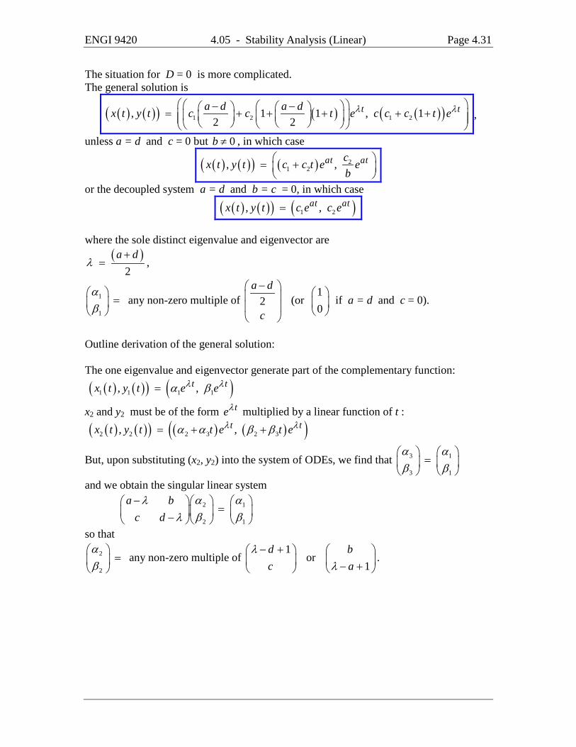
The situation for D = 0 is more complicated. The general solution is
( ) ( )( ) ( ) ( )( )1 2 1 2, 1 1 , 12 2
t ta d a dx t y t c c t e c c c t eλ λ − − = + + + + + ,
unless a = d and c = 0 but 0b ≠ , in which case
( ) ( )( ) ( ) 21 2, ,at atcx t y t c c t e e
b = +
or the decoupled system a = d and b = c = 0, in which case
( ) ( )( ) ( )1 2, ,at atx t y t c e c e= where the sole distinct eigenvalue and eigenvector are
( ) ,2
a dλ
+=
1
1
αβ
=
any non-zero multiple of 2a d
c
−
(or 10
if a = d and c = 0).
Outline derivation of the general solution: The one eigenvalue and eigenvector generate part of the complementary function:
( ) ( )( ) ( )1 1 1 1, ,t tx t y t e eλ λα β=
x2 and y2 must be of the form teλ multiplied by a linear function of t : ( ) ( )( ) ( ) ( )( )2 2 2 3 2 3, ,t tx t y t t e t eλ λα α β β= + +
But, upon substituting (x2, y2) into the system of ODEs, we find that 3 1
3 1
α αβ β
=
and we obtain the singular linear system
2 1
2 1
a bc d
α αλβ βλ
− = −
so that 2
2
αβ
=
any non-zero multiple of 1d
cλ − +
or 1
baλ
− +
.

ENGI 9420 4.06 - Linear Approximation (2) Page 4.32
4.06 Linear Approximation to a System of Non-Linear ODEs (2) From sections 4.02 and 4.03, the non-linear system
( ) ( ), , ,dx dyx P x y y Q x ydt dt
= = = = (1)
with critical point at (0, 0) may be expressed as
( )( )
1
1
,
,
x ax b y P x y
y cx d y Q x y
= + +
= + +
(2)
where a, b, c, d are all constants and
( ) ( )
( )( ) ( )
( )1 1
2 2 2 2, 0,0 , 0,0
, ,lim 0 and lim 0
x y x y
P x y Q x y
x y x y→ →= =
+ +.
Near the critical point (0, 0), this system may be approximated by the linear system
x ax b yy cx d y= += +
(3)
Effect of Small Perturbations Small perturbations in the values of the coefficients a, b, c, d are reflected in small changes in the eigenvalues λ. If the eigenvalues are a pure imaginary pair, λ = ± jv, then the critical point is a centre. The effect of small changes in the coefficients will change the eigenvalues to the complex conjugate pair λ' = u' ± jv', where u' is small in magnitude and v' is close to v.

ENGI 9420 4.06 - Linear Approximation (2) Page 4.33
If the eigenvalues are a real equal pair, λ1 = λ2, then a slight perturbation is likely to separate the roots into distinct values. If those values are still real, then the critical point remains a node. If the perturbed eigenvalues are a complex conjugate pair, then the nature of the trajectories will change into spirals and the critical point changes from a node into a focus. However, in both cases, an asymptotically stable critical point remains asymptotically stable after a small perturbation, while an unstable critical point remains unstable. In all other cases, a slight perturbation leaves the sign of the real part of both eigenvalues unchanged and affects neither the type of critical point nor the overall type of the orbits. These results are summarized in the two following theorems. Poincaré’s Theorem: The singularities of the non-linear system (2) are identical to the singularities of the linear system (3), except for the cases D < 0 and a + d = 0, which is a centre in the linear case, but may be a centre or a focus in the non-linear case; and D = 0, which is either a node or a focus in the non-linear case. Theorem on stability of the singularity at (0, 0): Linear approximation Non-linear system asymptotically stable unstable stable but not asymptotically stable
ENGI 9420 4.06 - Linear Approximation (2) Page 4.34
Example 4.06.1 Perform a stability analysis on the system
2 2, 2 6d x d yx x xy y xy ydt dt
= − + = − −

ENGI 9420 4.06 - Linear Approximation (2) Page 4.35
Example 4.06.1 (continued)

ENGI 9420 4.06 - Linear Approximation (2) Page 4.36
Example 4.06.1 (continued)

ENGI 9420 4.06 - Linear Approximation (2) Page 4.37
Example 4.06.1 (continued)
ENGI 9420 4.06 - Linear Approximation (2) Page 4.38
Example 4.06.1 (continued)
ENGI 9420 4.06 - Linear Approximation (2) Page 4.39
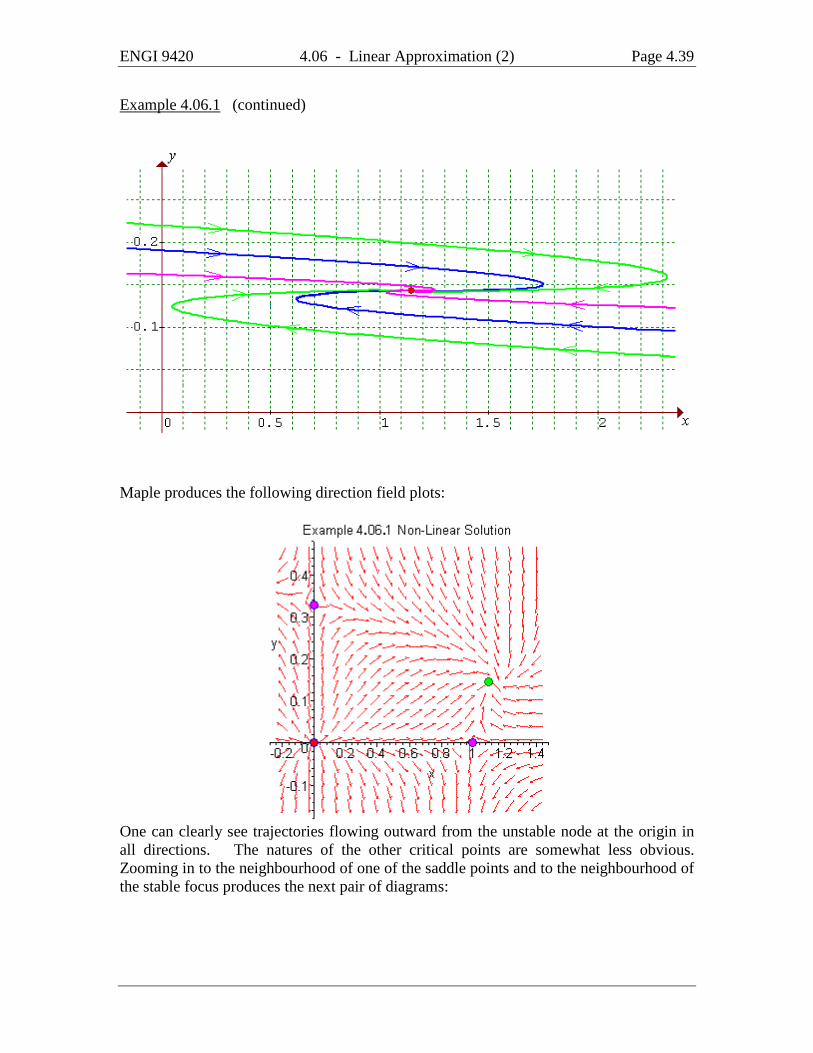
Example 4.06.1 (continued)
Maple produces the following direction field plots:
One can clearly see trajectories flowing outward from the unstable node at the origin in all directions. The natures of the other critical points are somewhat less obvious. Zooming in to the neighbourhood of one of the saddle points and to the neighbourhood of the stable focus produces the next pair of diagrams:
ENGI 9420 4.06 - Linear Approximation (2) Page 4.40
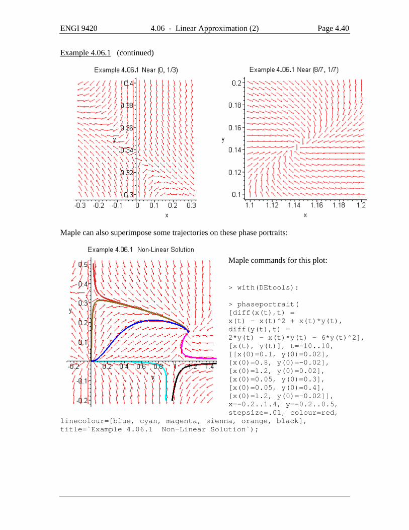
Example 4.06.1 (continued)
Maple can also superimpose some trajectories on these phase portraits:
Maple commands for this plot: > with(DEtools): > phaseportrait( [diff(x(t),t) = x(t) - x(t)^2 + x(t)*y(t), diff(y(t),t) = 2*y(t) - x(t)*y(t) - 6*y(t)^2], [x(t), y(t)], t=-10..10, [[x(0)=0.1, y(0)=0.02], [x(0)=0.8, y(0)=-0.02], [x(0)=1.2, y(0)=0.02], [x(0)=0.05, y(0)=0.3], [x(0)=0.05, y(0)=0.4], [x(0)=1.2, y(0)=-0.02]], x=-0.2..1.4, y=-0.2..0.5, stepsize=.01, colour=red,
linecolour=[blue, cyan, magenta, sienna, orange, black], title=`Example 4.06.1 Non-Linear Solution`);
ENGI 9420 4.06 - Linear Approximation (2) Page 4.41
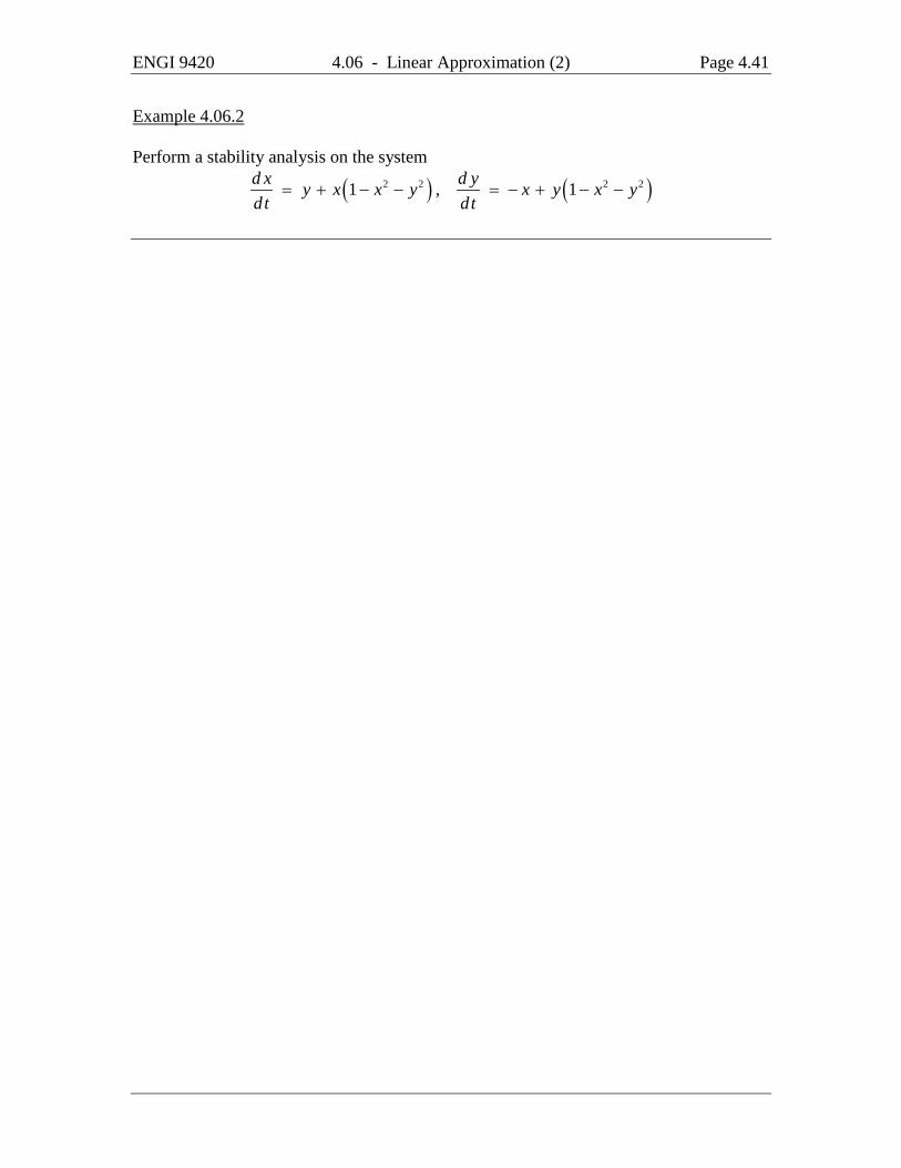
Example 4.06.2 Perform a stability analysis on the system
( ) ( )2 2 2 21 , 1d x d yy x x y x y x ydt dt
= + − − = − + − −

ENGI 9420 4.06 - Linear Approximation (2) Page 4.42
Example 4.06.2 (continued)
Solution in the neighbourhood of the only critical point (0, 0):
Now consider the distance r of any point (x, y) from the critical point (0, 0):
2 2 2 2 drr x y rdt
= + ⇒ =
ENGI 9420 4.06 - Linear Approximation (2) Page 4.43
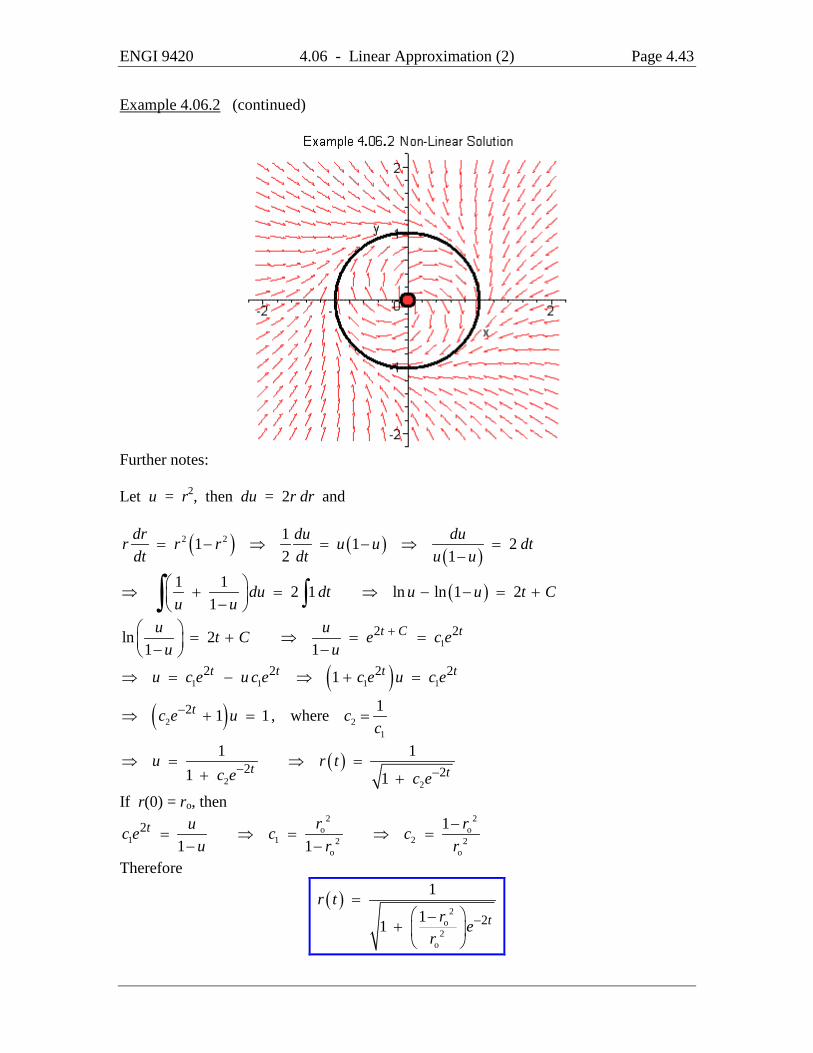
Example 4.06.2 (continued)
Further notes: Let u = r2, then du = 2r dr and
( ) ( ) ( )2 2 11 1 2
2 1dr du dur r r u u dtdt dt u u
= − ⇒ = − ⇒ =−
( )1 1 2 1 ln ln 1 21
du dt u u t Cu u
⇒ + = ⇒ − − = + − ∫∫
12 2ln 2
1 1t C tu ut C e c e
u u+ = + ⇒ = = − −
( )1 1 1 12 2 2 21t t t tu c e u c e c e u c e⇒ = − ⇒ + =
( )2 21
2 11 1, wheretc e u cc
−⇒ + = =
( )2 2
2 21 1
1 1t t
u r tc e c e
− −⇒ = ⇒ =
+ +
If r(0) = ro, then 2 2
o o1 1 22 2
o o
2 11 1
t r ruc e c cu r r
−= ⇒ = ⇒ =
− −
Therefore
( )2
o2
o
2
1
11 tr t
r er
−=
−+
ENGI 9420 4.06 - Linear Approximation (2) Page 4.44
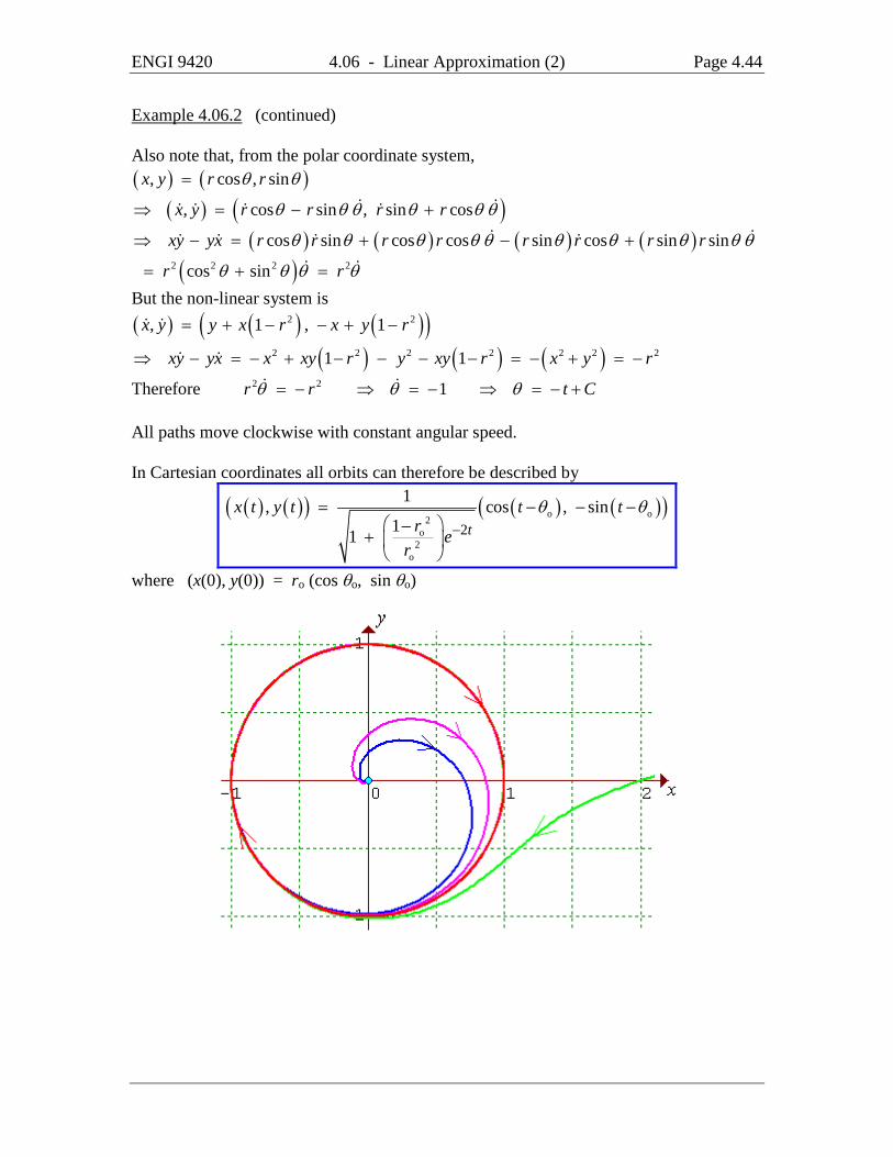
Example 4.06.2 (continued) Also note that, from the polar coordinate system, ( ) ( ), cos , sinx y r rθ θ=
( ) ( ), cos sin , sin cosx y r r r rθ θ θ θ θ θ⇒ = − +
( ) ( ) ( ) ( )cos sin cos cos sin cos sin sinxy yx r r r r r r r rθ θ θ θ θ θ θ θ θ θ⇒ − = + − +
( )2 2 2 2cos sinr rθ θ θ θ= + = But the non-linear system is ( ) ( ) ( )( )2 2, 1 , 1x y y x r x y r= + − − + −
( ) ( ) ( )2 2 2 2 2 2 21 1xy yx x xy r y xy r x y r⇒ − = − + − − − − = − + = −
Therefore 2 2 1r r t Cθ θ θ= − ⇒ = − ⇒ = − + All paths move clockwise with constant angular speed. In Cartesian coordinates all orbits can therefore be described by
( ) ( )( ) ( ) ( )( )o o2o
2o
2
1, cos , sin11 t
x t y t t tr e
r
θ θ−
= − − − −
+
where (x(0), y(0)) = ro (cos θo, sin θo)
ENGI 9420 4.06 - Linear Approximation (2) Page 4.45
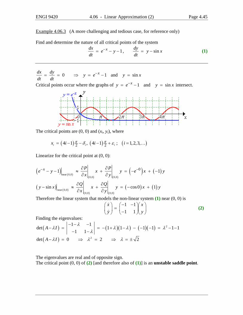
Example 4.06.3 (A more challenging and tedious case, for reference only) Find and determine the nature of all critical points of the system
1 , sinxdx dye y y xdt dt
−= − − = − (1)
0 1 and sinxdx dy y e y xdt dt
−= = ⇒ = − =
Critical points occur where the graphs of 1 and sinxy e y x−= − = intersect.
The critical points are (0, 0) and (xi, yi), where ( ) ( ) ( )2 24 1 , 4 1 ; 1,2,3,i i ix i i iπ πδ ε= − − − + = Linearize for the critical point at (0, 0):
( )( )
( ) ( )( ) ( )
near 0,00,0 0,0
01 1x P Pe y x y e x yx y
− −∂ ∂− − ≈ + = − + −
∂ ∂
( ) ( )( ) ( )
( ) ( )near 0,0
0,0 0,0
sin cos 0 1Q Qy x x y x yx y
∂ ∂− ≈ + = − +
∂ ∂
Therefore the linear system that models the non-linear system (1) near (0, 0) is
1 11 1
x xy y
− − = −
(2)
Finding the eigenvalues:
( ) ( )( ) ( )( ) 21 1det 1 1 1 1 1 1
1 1A I
λλ λ λ λ
λ− − −
− = = − + − − − − = − −− −
( ) 2det 0 2 2A Iλ λ λ− = ⇒ = ⇒ = ± The eigenvalues are real and of opposite sign. The critical point (0, 0) of (2) [and therefore also of (1)] is an unstable saddle point.
ENGI 9420 4.06 - Linear Approximation (2) Page 4.46
Example 4.06.3 (continued) Using the results on page 4.30,
( ) ( ) ( )( )2 24 1 1 4 1 1 4 4 8D a d bc= − + = − − + − − = + = The eigenvectors are
1
1
αβ
=
any non-zero multiple of ( ) 2 2 2
for 2221
a d D
cλ
− − − − = = − −
and
2
2
αβ
=
any non-zero multiple of ( ) 2 2 2
for 2221
a d D
cλ
− + − + = = + −
Choose a multiple of –1 in both cases. The general solution of (2) is therefore
( ) ( )( ) ( ) ( )( )1 2 1 22 2 2 2, 1 2 1 2 ,t t t tx t y t c e c e c e c e− −= + + − +
( )( )
1 1 2lim 2 1 01 21 2t
y tx t→−∞
−= = = − >
−+ and
( )( )
1 1 2lim 1 2 01 21 2t
y tx t→+∞
+= = = − − <
−−
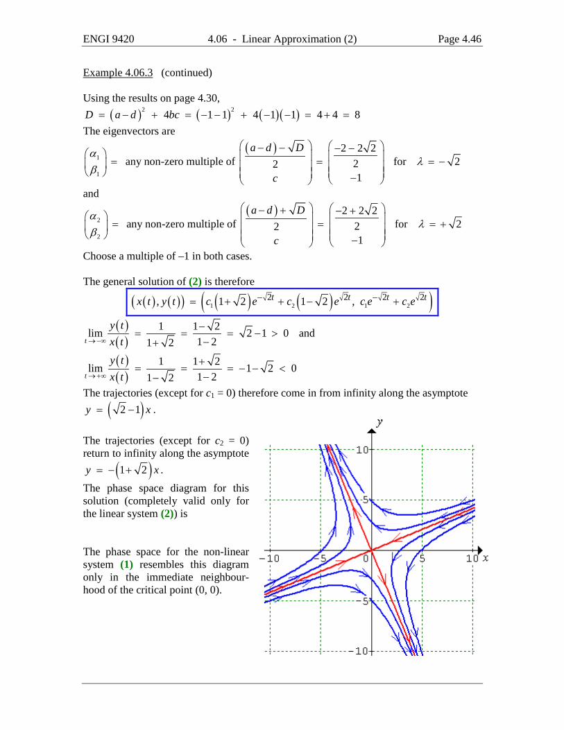
The trajectories (except for c1 = 0) therefore come in from infinity along the asymptote
( )2 1y x= − .
The trajectories (except for c2 = 0) return to infinity along the asymptote
( )1 2y x= − + .
The phase space diagram for this solution (completely valid only for the linear system (2)) is The phase space for the non-linear system (1) resembles this diagram only in the immediate neighbour-hood of the critical point (0, 0).
ENGI 9420 4.06 - Linear Approximation (2) Page 4.47
Example 4.06.3 (continued) At other critical points (k, l),
0 sin sin 1 0kdx dy l k e kdt dt
−= = ⇒ = ⇒ − − =
Linearizing (Taylor’s series for P(x, y) about (x, y) = (k, l):
( )( )
( )( )
( )( ) ( )( ) ( )( )
near ,, ,
1 1k l
k l k l
x kP Pe y x k y l e x k y lx y
− −∂ ∂− − ≈ − + − = − − + − −
∂ ∂
( ) ( )( )
( )( )
( ) ( )( ) ( )( )near ,
, ,
sin cos 1k l
k l k l
Q Qy x x k y l k x k y lx y
∂ ∂− ≈ − + − = − − + −
∂ ∂
Therefore the linear system that models the non-linear system (1) near (k, l) is
1cos 1
kx x key y lk
− − − −= −−
(3)
Finding the eigenvalues:
( ) ( )( ) ( )( )1det 1 cos 1cos 1
kkeA I e k
kλλ λ λ
λ
−−− − −− = = − + − − − −
− −
( ) ( )2 1 cos 0k ke e kλ λ− −= − − − + =
( ) ( ) ( )21 1 4 cos
2
k k ke e e kλ
− − −− ± − + +⇒ =
( ) ( )21 1 4cos
2
k ke e kλ
− −− ± + +⇒ =
Now 0 0 1 0 1 1k kk e e− −> ⇒ < < ⇒ < − < Recall that ( ) ( ) ( )2 24 1 , 4 1 ; 1,2,3,i i ik x i i iπ πδ ε= = − − − + = Examining the right-hand critical point in each pair,
( ) ( )24 1 , 0 1i ik i π ε ε= − + <
( )( ) ( ) ( )2 2 2cos cos 4 1 cos cos sin 0i i i i ik i π π πε ε ε ε ε⇒ = − + = − = − = ≈ >
Therefore ( ) ( ) ( )21 4 cos 1 0k k ke e k e− − −− + + > − >
and the two eigenvalues are real and of opposite sign. These critical points are therefore all unstable saddle points.
ENGI 9420 4.06 - Linear Approximation (2) Page 4.48
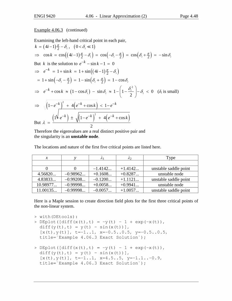
Example 4.06.3 (continued) Examining the left-hand critical point in each pair,
( ) ( )24 1 , 0 1i ik i π δ δ= − − <
( )( ) ( ) ( )2 2 2cos cos 4 1 cos cos sini i i ik i π π πδ δ δ δ⇒ = − − = − − = + = −
But k is the solution to sin 1 0ke k− − − =
( )( )21 sin 1 sin 4 1 ike k i π δ−⇒ = + = + − −
( ) ( )2 21 sin 1 sin 1 cosi i iπ πδ δ δ= + − − = − + = −
( )2
cos 1 cos sin 1 1 02i
i i ike k δδ δ δ−
⇒ + ≈ − − ≈ − − − <
(δi is small)
( ) ( )21 4 cos 1k k ke e k e− − −⇒ − + + < −
But ( ) ( ) ( )21 1 4 cos
2
k k ke e e kλ
− − −− ± − + +=
Therefore the eigenvalues are a real distinct positive pair and the singularity is an unstable node. The locations and nature of the first five critical points are listed here.
x y λ1 λ2 Type 0 0 –1.4142... +1.4142... unstable saddle point
4.56820... –0.98962... +0.1608... +0.8287... unstable node 4.83833... –0.99208... –0.1200... +1.1121... unstable saddle point 10.98977... –0.99998... +0.0058... +0.9941... unstable node 11.00135... –0.99998... –0.0057... +1.0057... unstable saddle point
Here is a Maple session to create direction field plots for the first three critical points of the non-linear system. > with(DEtools): > DEplot([diff(x(t),t) = -y(t) - 1 + exp(-x(t)), diff(y(t),t) = y(t) - sin(x(t))], [x(t),y(t)], t=-1..1, x=-0.5..0.5, y=-0.5..0.5, title=`Example 4.06.3 Exact Solution`); > DEplot([diff(x(t),t) = -y(t) - 1 + exp(-x(t)), diff(y(t),t) = y(t) - sin(x(t))], [x(t),y(t)], t=-1..1, x=4.5..5, y=-1.1..-0.9, title=`Example 4.06.3 Exact Solution`);
ENGI 9420 4.06 - Linear Approximation (2) Page 4.49
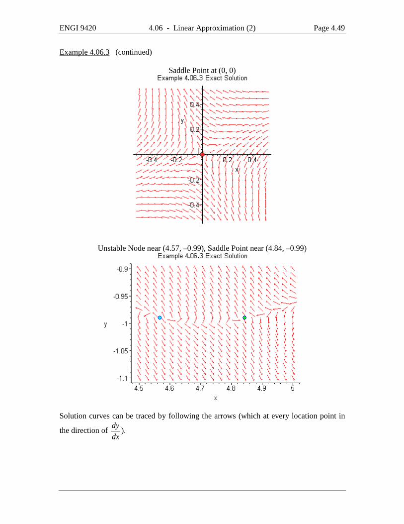
Example 4.06.3 (continued)
Saddle Point at (0, 0)
Unstable Node near (4.57, –0.99), Saddle Point near (4.84, –0.99)
Solution curves can be traced by following the arrows (which at every location point in
the direction of dydx
).

ENGI 9420 4.07 - Limit Cycles Page 4.50
4.07 Limit Cycles If, in some region, all trajectories begin on a closed curve inside that region, then that curve is an unstable limit cycle.
If all trajectories terminate on the curve, then it is a stable limit cycle.
More formally, Let R be a bounded region in the xy plane. Let C be a closed curve composed of interior points of R and bounding a region A. Let C be a solution curve of the system
( ) ( ), , ,dx dyx P x y y Q x ydt dt
= = = = (1)
where P(x, y) and Q(x, y) are differentiable with respect to x and y at all points of R. C is a limit cycle of (1) if no other closed solution curve is close to C and if all orbits sufficiently near it approach it asymptotically as t → –∞ (unstable) or as t → +∞ (stable). Bendixon Non-existence Theorem:
For system (1), if the expression P Qx y
∂ ∂+
∂ ∂ does not change sign or vanish identically in
a simply connected (= "no holes") region D inside R, then no closed trajectory can exist entirely within D. The contrapositive statement is:
If C is a closed solution curve of (1) in R, then P Qx y
∂ ∂+
∂ ∂ must vanish for some subset
of R.

ENGI 9420 4.07 - Limit Cycles Page 4.51
Proof: If C is a closed curve in R with interior region A, then Green’s theorem in two dimensions states
( )C A
P QP dy Q dx dx dyx y
∂ ∂− = + ∂ ∂ ∫ ∫∫ (2)
Poincaré-Bendixon Theorem (Existence Theorem for Limit Cycles) If the solution curve C of the system (1) is in and remains in a bounded region R for t > to without approaching singular points and if P(x, y) and Q(x, y) are differentiable with respect to x and y at all points of R, then a limit cycle exists in R and either C is a limit cycle or it approaches a limit cycle as t → +∞.
ENGI 9420 4.08 - Van der Pol’s ODE Page 4.52
4.08 Van der Pol’s Equation During an investigation of the properties of vacuum tubes, Van der Pol developed a second order non-linear ordinary differential equation to model the circuit:
( ) ( )2
22 1 0 , 0d x dxx x
dt dtµ µ− − + = > (1)
The linear form resembles the linear ODE for the RLC circuit:
2
2
1 0d i R di idt L dt LC
+ + = (2)
The resistance term in (2) provides damping provided R > 0. If R < 0, then the solution is unstable and the current would have an ever increasing amplitude, which is what the linear form of (1) predicts, (–µ < 0). However, experimental evidence suggests that, after some initial increase in amplitude, a periodic solution is attained. This is an indication that a limit cycle may exist for (1). The “resistance” term –µ (1 – x2) in Van der Pol’s equation is negative if | x | < 1, but is positive for | x | > 1. The non-linear term must be retained in order to find the periodic steady state solution. Introduce a new variable y to Van der Pol’s equation:
( )21
dx ydtdy x y xdt
µ
=
= − − (3)
The linear version of (3) is:
0 11
x xy yµ
= −
(4)
Finding the critical points of (3):

ENGI 9420 4.08 - Van der Pol’s ODE Page 4.53
ENGI 9420 4.08 - Van der Pol’s ODE Page 4.54
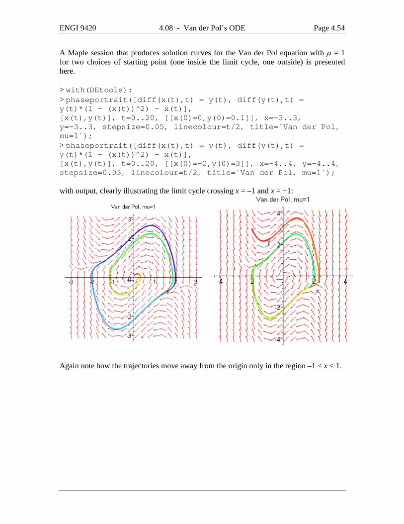
A Maple session that produces solution curves for the Van der Pol equation with µ = 1 for two choices of starting point (one inside the limit cycle, one outside) is presented here. > with(DEtools): > phaseportrait([diff(x(t),t) = y(t), diff(y(t),t) = y(t)*(1 - (x(t))^2) - x(t)], [x(t),y(t)], t=0..20, [[x(0)=0,y(0)=0.1]], x=-3..3, y=-3..3, stepsize=0.05, linecolour=t/2, title=`Van der Pol, mu=1`); > phaseportrait([diff(x(t),t) = y(t), diff(y(t),t) = y(t)*(1 - (x(t))^2) - x(t)], [x(t),y(t)], t=0..20, [[x(0)=-2,y(0)=3]], x=-4..4, y=-4..4, stepsize=0.03, linecolour=t/2, title=`Van der Pol, mu=1`); with output, clearly illustrating the limit cycle crossing x = –1 and x = +1:
Again note how the trajectories move away from the origin only in the region –1 < x < 1.
ENGI 9420 4.09 - Theorem for Limit Cycles Page 4.55
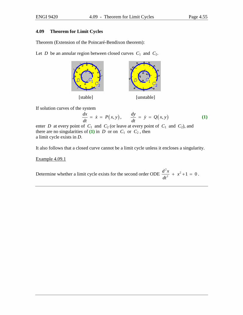
4.09 Theorem for Limit Cycles Theorem (Extension of the Poincaré-Bendixon theorem): Let D be an annular region between closed curves C1 and C2. [stable] [unstable] If solution curves of the system
( ) ( ), , ,dx dyx P x y y Q x ydt dt
= = = = (1)
enter D at every point of C1 and C2 (or leave at every point of C1 and C2), and there are no singularities of (1) in D or on C1 or C2 , then a limit cycle exists in D. It also follows that a closed curve cannot be a limit cycle unless it encloses a singularity. Example 4.09.1
Determine whether a limit cycle exists for the second order ODE 2
22 1 0d x x
dt+ + = .
ENGI 9420 4.09 - Theorem for Limit Cycles Page 4.56
Example 4.09.2 Perform a stability analysis and determine whether a limit cycle exists for the system
( )
( )
2 2
2 2
1 5
5 1
dx x x y ydtdy x y x ydt
= − − +
= − + − − (1)

ENGI 9420 4.09 - Theorem for Limit Cycles Page 4.57
Example 4.09.2 (continued)
ENGI 9420 4.09 - Theorem for Limit Cycles Page 4.58
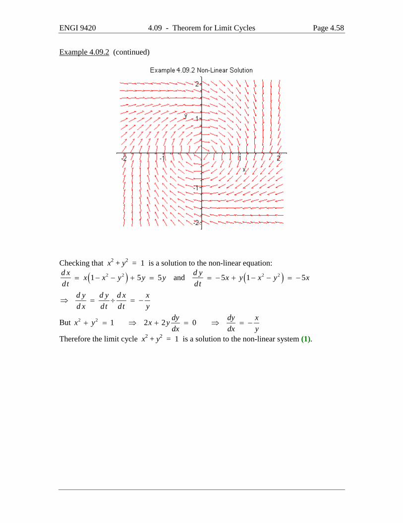
Example 4.09.2 (continued)
Checking that x2 + y2 = 1 is a solution to the non-linear equation:
( ) ( )2 2 2 21 5 5 and 5 1 5d x d yx x y y y x y x y xdt dt
= − − + = = − + − − = −
d y d y d x xd x dt dt y
⇒ = ÷ = −
But 2 2 1 2 2 0dy dy xx y x ydx dx y
+ = ⇒ + = ⇒ = −
Therefore the limit cycle x2 + y2 = 1 is a solution to the non-linear system (1).
ENGI 9420 4.10 - Lyapunov Functions Page 4.59
4.10 Lyapunov Functions [for reference only - not examinable] The equation of motion for an unforced damped elastic mass-spring system is
2
2 0d x d x xdt dt
ε µ+ + = (1)
Consider the case where the restoring force (per unit mass) coefficient µ = 1 and the damping (per unit mass) coefficient ε is small and positive. The equivalent first order system is
d x ydtd y x ydt
ε
=
= − − (2)
The coefficient matrix is 0 11
Aε
= − −
Using the results on page 4.30, ( ) ( ) ( )( )2 2 24 0 4 1 1 4 0D a d bc ε ε= − + = + + − = − <
( ) 242 2
a d D jε ελ
+ ± − ± −= =
[or solve the characteristic equation det(A – λI) = 0: ( )( ) ( )( ) 20 1 1 0 1 0λ ε λ λ ελ− − − − − = ⇒ − + = .] The single critical point at the origin is therefore a stable focus (asymptotically stable).

ENGI 9420 4.10 - Lyapunov Functions Page 4.60
The kinetic energy is 2
2 21 1 12 2 2
dxmv m mydt
= =
.
The potential energy of a mass-spring system is proportional to the square of the extension x. Therefore the function ( ) ( )2 21
2,V x y x y= + is related to the total energy of the system. V(x, y) has an absolute minimum value of 0 at the origin, which should therefore be a stable equilibrium point. From the chain rule and (2),
( ) 2 0dV V dx V dy x y y x y y tdt x dt y dt
ε ε∂ ∂= + = ⋅ + − − = − ≤ ∀
∂ ∂
Therefore V decreases as t increases. Also V decreases as the distance from the origin decreases. Therefore the distance from the origin must decrease as t increases.
( ) ( )lim lim 0t t
x t y t→∞ →∞
= = . All orbits terminate at the origin.
Again, the origin is an asymptotically stable point. Energy considerations and Stability: For a system of differential equations that arises from the description of a physical system, if the total energy of the system is constant or decreasing and a critical point corresponds to a point of minimum potential energy of the system, then the critical point should be stable. If the critical point corresponds to a maximum of potential energy (such as the upside-down position of the pendulum in section 4.01), then the critical point should be unstable. If (0, 0) is an asymptotically stable critical point of the system
( ) ( ), , ,dx dyf x y g x ydt dt
= = (3)
then there must exist some domain D, containing (0, 0), such that all solutions in D must approach (0, 0) as t → ∞. Suppose that an energy function V(x, y) exists such that V(0, 0) = 0 and V(x, y) > 0 everywhere else in D. Then, following any open orbit in D, V must decrease to zero as t → ∞. The converse of these statements is more useful: If V decreases to zero as t → ∞ on every trajectory in D, then every trajectory in D must approach the origin as t → ∞ and the origin is therefore asymptotically stable.

ENGI 9420 4.10 - Lyapunov Functions Page 4.61
Definitions: Let V(x, y) be defined on some domain D that contains the origin. V is positive definite on D if V(0, 0) = 0 and V(x, y) > 0 for all other points in D. V is negative definite on D if V(0, 0) = 0 and V(x, y) < 0 for all other points in D. V is positive semi-definite on D if V(0, 0) = 0 and V(x, y) ≥ 0 for all other points in D. V is negative semi-definite on D if V(0, 0) = 0 and V(x, y) ≤ 0 for all other points in D. A function V(x, y) is a Lyapunov function for the system
( ) ( ), , ,dx dyf x y g x ydt dt
= = (3)
if there exists some neighbourhood of the origin in which • V is a differentiable function of x and y; • V > 0 except at the origin, where V = 0; and
• For any solution (x(t), y(t)) of (3) there exists a to such that 0dVdt
≤ for all t > to.
Theorem: If V(x, y) is a Lyapunov function for the system (3), then:
If dVdt
is negative semidefinite, then (0, 0) is stable.
If dVdt
is negative definite, then (0, 0) is asymptotically stable.
If dVdt
is positive definite, then (0, 0) is unstable.

ENGI 9420 4.10 - Lyapunov Functions Page 4.62
Also note that, by the chain rule and (3),
( ) ( ), ,dV V dx V dy V Vf x y g x ydt x dt y dt x y
∂ ∂ ∂ ∂= + = ⋅ + ⋅
∂ ∂ ∂ ∂
and that dV Vdt
= T
∇
where ˆ ˆV VVx y
∂ ∂= +
∂ ∂i j
∇ is the gradient vector of the scalar function V(x, y) and
( ) ( )ˆ ˆ ˆ ˆ, ,dx dy f x y g x ydt dt
= + = +T i j i j
is the tangent vector to the trajectory
(x(t), y(t)).
If dVdt
is negative definite, then the two vectors
must point in directions more than 90° apart, everywhere in the region (except possibly at the origin). But the gradient vector points in the direction of increasing V, at right angles to the contours V = constant. V is positive definite, so its gradient vector points outward, away from the origin. Therefore the trajectories must point inward, everywhere in the region where V is positive
definite and dVdt
is negative definite.
The general quadratic function
( ) 2 2,V x y ax b x y c y= + + is positive definite if and only if a > 0 and b2 – 4ac < 0 and is negative definite if and only if a < 0 and b2 – 4ac < 0
ENGI 9420 4.10 - Lyapunov Functions Page 4.63
Example 4.10.1 The populations of a pair of competing species are modelled by the system
( )
( )
1
0.75 0.5
dx x x ydtdy y y xdt
= − −
= − −
Investigate the stability of the critical point at (0.5, 0.5). Transform the critical point to the origin with the change of coordinates
w = x – 0.5 ; z = y – 0.5 The system becomes
( ) ( ) ( )( )
( ) ( ) ( )( )
2
2
0.5 1 0.5 0.5 0.5 0.5
0.5 0.75 0.5 0.5 0.5 0.25 0.5 0.5
dw w w z w z w wzdtdz z z w w z wz zdt
= + − + − + = − − − −
= + − + − + = − − − −
There are many possible choices for a Lyapunov function, among the simplest of which is
V(w, z) = w2 + z2 V is clearly positive definite: V(0, 0) = 0 and V(w, z) > 0 everywhere else. dV V dw V dzdt w dt z dt
∂ ∂= ⋅ + ⋅
∂ ∂
( ) ( )2 22 0.5 0.5 2 0.25 0.5 0.5w w z w wz z w z wz z= − − − − + − − − −
( ) ( )2 2 3 2 2 31.5 2 2 2w wz z w w z wz z= − + + − + + +
In the quadratic expression ( )2 21.5w wz z− + + , a = c = –1 and b = –1.5.
a < 0 and b2 – 4ac < 0, so that ( )2 21.5w wz z− + + is negative definite. The cubic terms can be of either sign, but sufficiently close to (w, z) = (0, 0) they will be negligible compared to the quadratic terms. Therefore a region does exist around (0, 0)
such that V is positive definite and dVdt
is negative definite. The critical point must
therefore be asymptotically stable. By using a more complicated Lyapunov function and obtaining bounds on where its derivative is negative definite, one can estimate how far the region of asymptotic stability extends around the critical point.

ENGI 9420 4.10 - Lyapunov Functions Page 4.64
Example 4.10.1 (continued) Note that we can also investigate stability by finding the eigenvalues of the linear system that approximates the non-linear system near the critical point:
0.5 0.5 0.50.25 0.5 0.5
x xy y
− − − = − − −
The characteristic equation is ( ) ( ) ( )( )2det 0 0.5 0.5 0.25 0A Iλ λ− = ⇒ − − − − − =
( )20.5 0.125 0.5 0.125 0.5 0.125λ λ λ⇒ + = ⇒ + = ± ⇒ = − ± which is a real distinct negative pair. The critical point is therefore an asymptotically stable node.
ENGI 9420 4.11 - Duffing’s Equation Page 4.65
4.11 Duffing’s Equation Among the simplest models of damped non-linear forced oscillations of a mechanical or electrical system with a cubic stiffness term is Duffing’s equation:
2
32 cosd x dxa b x c x d t
dt dtω+ + + = (1)
In section 4.01, we considered the simple undamped pendulum:
2
2 sin 0d x g xdt L
+ = (2)
When x is very small, sin x ≈ x and (2) reduces to the ODE for simple harmonic motion.
The next order approximation is 3
sin6xx x≈ − , so that (2) becomes
2 3
2 06
d x g g xxdt L L
+ − = (3)
If we add a damping term dxadt
and a forcing function d cos ωt , then (3) becomes
Duffing’s equation (1).

ENGI 9420 4.11 - Duffing’s Equation Page 4.66
Special Case 1: Conduct a stability analysis for the undamped unforced Duffing’s equation
2
2 32 0d x x c x
dtω+ + = (4)
The equivalent first order system is
2 3
dx ydtdy x c xdt
ω
=
= − − (5)
Critical points:

ENGI 9420 4.11 - Duffing’s Equation Page 4.67
Special Case 1: (continued)

ENGI 9420 4.11 - Duffing’s Equation Page 4.68
Exact Solution of Special Case 1: The system (5),
2 3
dx ydtdy x c xdt
ω
=
= − −
dydx
⇒ =
ENGI 9420 4.11 - Duffing’s Equation Page 4.69
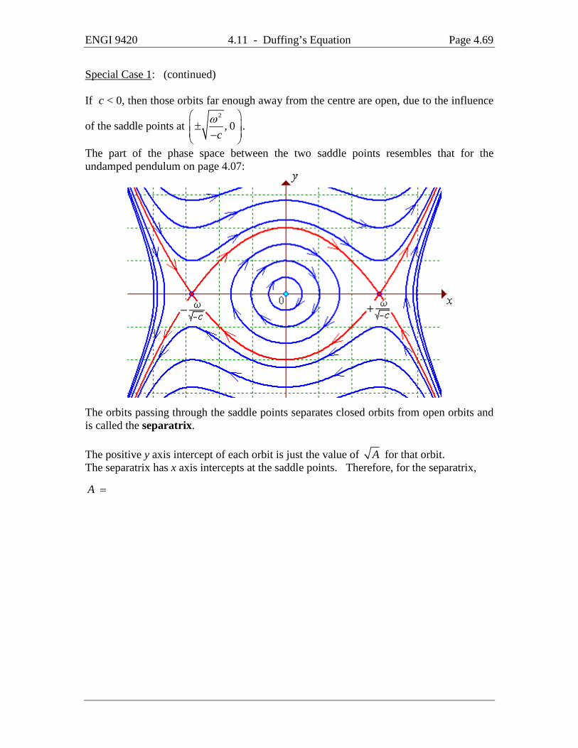
Special Case 1: (continued) If c < 0, then those orbits far enough away from the centre are open, due to the influence
of the saddle points at 2
, 0c
ω ± −
.
The part of the phase space between the two saddle points resembles that for the undamped pendulum on page 4.07:
The orbits passing through the saddle points separates closed orbits from open orbits and is called the separatrix. The positive y axis intercept of each orbit is just the value of A for that orbit. The separatrix has x axis intercepts at the saddle points. Therefore, for the separatrix,
A =
ENGI 9420 4.11 - Duffing’s Equation Page 4.70
Special Case 2: Conduct a stability analysis for the damped unforced Duffing’s equation
2
2 32 0d x dxa x c x
dt dtω+ + + = (8)
The equivalent first order system is
2 3
dx ydtdy x c x a ydt
ω
=
= − − − (9)
The critical points are the same as in special case 1:
( )2
20 and 0 ory x xcω
= = = −
Near (0, 0) the linear approximation is
2
0 1x xy a yω
= − −
(10)
The characteristic equation is det(A - λI) = 0 ⇒ λ 2 + aλ + ω 2 = 0 2 24
2a a ωλ − ± −
⇒ =
The critical point is stable if a > 0 and unstable if a < 0. It is a focus if a2 – 4ω 2 < 0 and a node otherwise. If c > 0, then this is the only critical point of (8).
If c < 0, then there are two other critical points, at 2
, 0c
ω ± −
.
ENGI 9420 4.11 - Duffing’s Equation Page 4.71
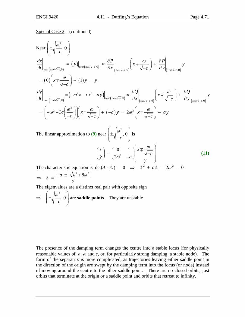
Special Case 2: (continued)
Near 2
, 0c
ω ± −
( )( ) ( )
( ) ( )near / ,
near / , / , / ,0
0 0 0c
c c c
dx P Py x ydt x ycω
ω ω ω
ω± −
± − ± − ± −
∂ ∂ = ≈ + ∂ ∂−
( ) ( )0 1x y yc
ω = + = −
( )( ) ( ) ( ) ( )
( )
2 3
near / ,near / , / , / ,
22 2
00 0 0
3 2
cc c c
dy Q Qx cx a y x ydt x yc
c x a y x a yc c c
ωω ω ω
ωω
ω ω ωω ω
± −± − ± − ± −
∂ ∂ = − − − ≈ + ∂ ∂−
= − − + − = − − − −
The linear approximation to (9) near 2
, 0c
ω ± −
is
2
0 12
xxc
y ay
ω
ω
= − −
(11)
The characteristic equation is det(A - λI) = 0 ⇒ λ 2 + aλ – 2ω 2 = 0 2 28
2a a ωλ − ± +
⇒ =
The eigenvalues are a distinct real pair with opposite sign
⇒ 2
, 0c
ω ± −
are saddle points. They are unstable.
The presence of the damping term changes the centre into a stable focus (for physically reasonable values of a, ω and c, or, for particularly strong damping, a stable node). The form of the separatrix is more complicated, as trajectories leaving either saddle point in the direction of the origin are swept by the damping term into the focus (or node) instead of moving around the centre to the other saddle point. There are no closed orbits; just orbits that terminate at the origin or a saddle point and orbits that retreat to infinity.
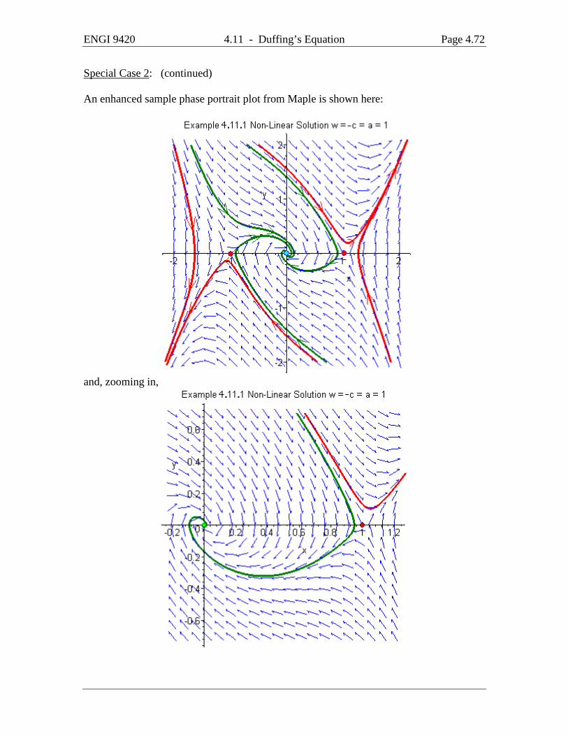
ENGI 9420 4.11 - Duffing’s Equation Page 4.72
Special Case 2: (continued) An enhanced sample phase portrait plot from Maple is shown here:
and, zooming in,

ENGI 9420 4.12 - More Examples Page 4.73
4.12 More Examples Example 4.12.1 Examine the stability of the linear second order differential equation
( )2
22 2 4 1 0d x dx x
dt dtπ+ + + =
and find the complete solution for the initial conditions ( ) ( ) ( )0 0 , 0 0 2x y x π= = = .
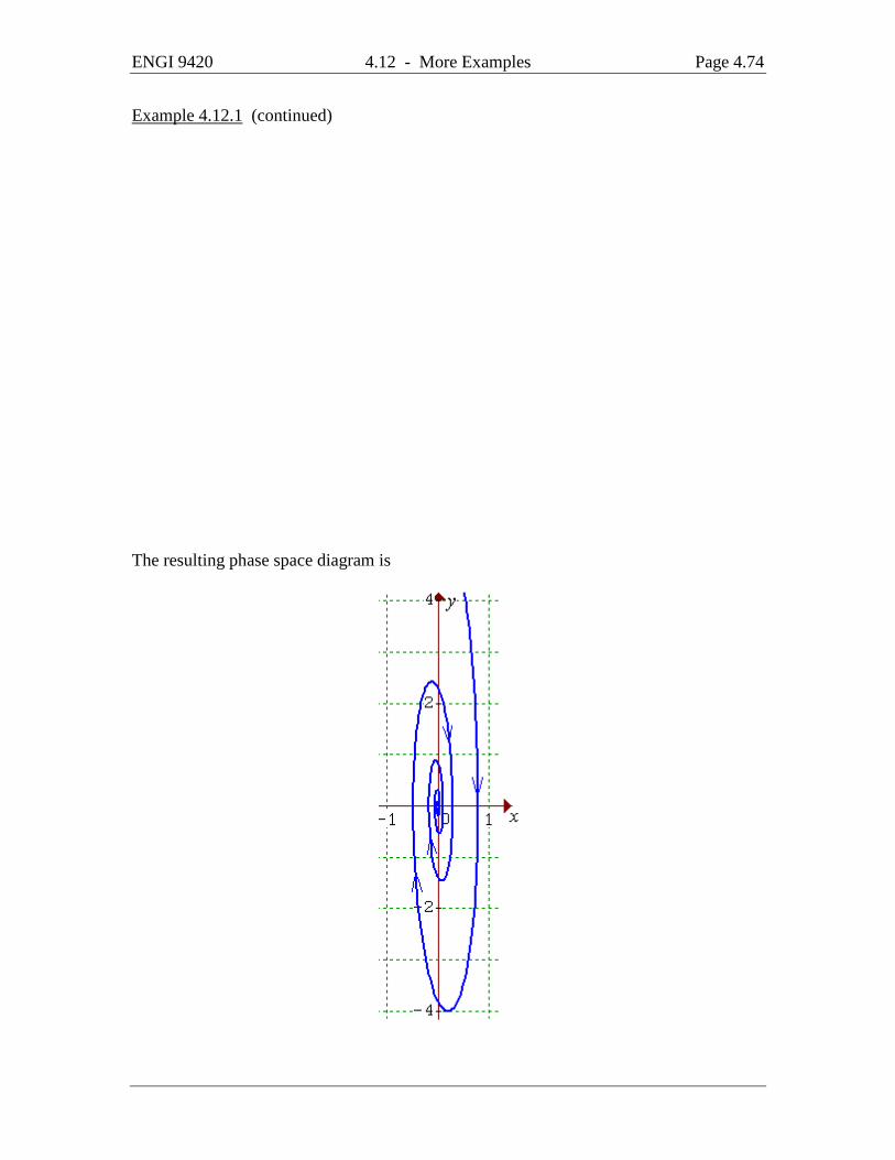
ENGI 9420 4.12 - More Examples Page 4.74
Example 4.12.1 (continued) The resulting phase space diagram is
ENGI 9420 4.12 - More Examples Page 4.75
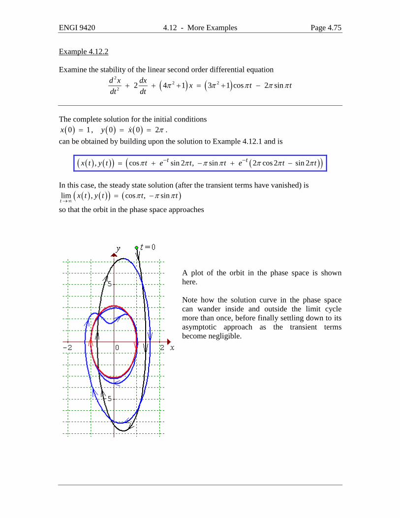
Example 4.12.2 Examine the stability of the linear second order differential equation
( ) ( )2
2 22 2 4 1 3 1 cos 2 sind x dx x t t
dt dtπ π π π π+ + + = + −
The complete solution for the initial conditions ( ) ( ) ( )0 1, 0 0 2x y x π= = = .
can be obtained by building upon the solution to Example 4.12.1 and is
( ) ( )( ) ( )( ), cos sin 2 , sin 2 cos 2 sin 2t tx t y t t e t t e t tπ π π π π π π− −= + − + − In this case, the steady state solution (after the transient terms have vanished) is
( ) ( )( ) ( )lim , cos , sint
x t y t t tπ π π→∞
= −
so that the orbit in the phase space approaches
A plot of the orbit in the phase space is shown here. Note how the solution curve in the phase space can wander inside and outside the limit cycle more than once, before finally settling down to its asymptotic approach as the transient terms become negligible.
ENGI 9420 4.12 - More Examples Page 4.76
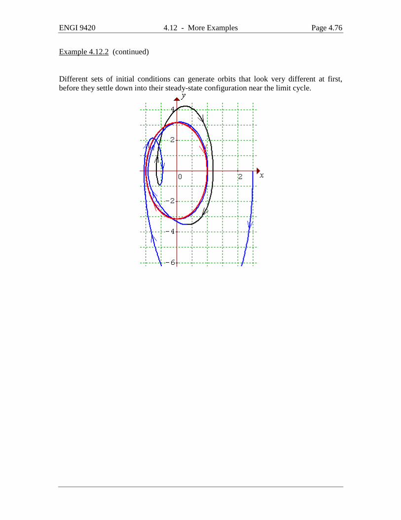
Example 4.12.2 (continued) Different sets of initial conditions can generate orbits that look very different at first, before they settle down into their steady-state configuration near the limit cycle.

ENGI 9420 4.13 - Liénard’s Theorem Page 4.77
4.13 Liénard’s Theorem If f (x) is an even function for all x and g(x) is an odd function for all x and g(x) > 0 for all x > 0
and ( ) ( )0
xF x f t dt= ∫ is such that F (x) = 0 has exactly one positive root, γ, and
F (x) < 0 for 0 < x < γ and F (x) > 0 and non-decreasing for x > γ, then the system
( ) ( ),x y y f x y g x= = − − or, equivalently,
( ) ( )2
2 0d x dxf x g xdt dt
+ + =
has a unique limit cycle enclosing the origin and that limit cycle is asymptotically stable. When all of the conditions of Liénard’s theorem are satisfied, the system has exactly one periodic solution, towards which all other trajectories spiral as t → ∞. Example 4.13.1 Let f (x) = –μ (1 – x2) and g(x) = x , (with μ > 0), then Liénard’s ODE becomes
( )2
22 1 0d x dxx x
dt dtµ− − + =
which is Van der Pol’s equation (section 4.08). Checking the conditions of Liénard’s theorem: f (x) = g(x) =
( )F x =
F (x) = 0 has only one positive root, γ =

ENGI 9420 4 - Stability Analysis Page 4.78
END OF CHAPTER 4
[Space for additional notes]