4 s B- 2: ns Unit B - 2: List of Subjects

AE301 Aerodynamics I

UNIT B: Theory of Aerodynamics

ROAD MAP . . .

B-1: Mathematics for Aerodynamics

B-2: Flow Field Representations

B-3: Potential Flow Analysis

B-4: Applications of Potential Flow Analysis

AE301 Aerodynamics I

Unit B-2: List of Subjects

Concept of Streamline

Strain and Angular Velocity

Angular Velocity and Vorticity

Rotational v.s. Irrotational Flows

Circulation of a Flow Field

Kutta-Joukowski Theorem

Stream Function

Velocity Potential

Inviscid and Incompressible Flow Equations

Laplace’s Equation

CONCEPT OF STREAMLINE

A streamline is a line whose tangent at any point is in the direction of the velocity vector at that point.

Mathematically, this means: d =s V 0 .

Let us examine this equation in 3-D Cartesian coordinate system:

ˆ ˆ ˆd dx dy dz= + +s i j k and ˆ ˆ ˆu v w= + +V i j k

Therefore, ( ) ( ) ( )

ˆ ˆ ˆ

ˆ ˆ ˆd dx dy dz wdy vdz udz wdx vdx udy

u v w

= = − + − + −

i j k

s V i j k

EQUATION OF STREAMLINE

In order to satisfy the condition of streamline: d =s V 0 , its each component must all equal to zero.

Therefore:

0wdy vdz− = (y-z plane) => dz w

dy v=

0udz wdx− = (x-z plane) => dz w

dx u=

0vdx udy− = (x-y plane) => dy v

dx u=

Unit B-2Page 1 of 15

Concept of Streamline

THE MOTION OF A FLUID ELEMENT

The motion of a fluid element along a streamline is a combination of “translation” and “rotation.”

In addition, the shape of the element can become “distorted” (“angular deformation”) as it moves.

• The presence of “viscosity” causes both “rotation” and “angular deformation,” and the flow field

is defined as “rotational flow.”

• If the viscosity within the flow field is ignored (“inviscid flow”), the motion of a fluid element can

be simplified only for “translation”: this is called, “irrotational flow.”

ANGULAR VELOCITY OF A FLUID ELEMENT (IN 2-D CARTESIAN: X-Y PLANE)


Strain and Angular Velocity

_________________________________________________________

_________________________________________________________

_________________________________________________________

_________________________________________________________

_________________________________________________________

_________________________________________________________

_________________________________________________________

_________________________________________________________

_________________________________________________________

_________________________________________________________

_________________________________________________________

_________________________________________________________

_________________________________________________________

_________________________________________________________

_________________________________________________________

_________________________________________________________

_________________________________________________________

_________________________________________________________

ANGULAR VELOCITY VECTOR OF A FLUID ELEMENT (3-D CARTESIAN)

Repeating a similar procedure in y-z and x-z planes, one can obtain:

1

2x

w v

y z

= −

(y-z plane) and

1

2y

u w

z x

= −

(x-z plane)

The angular velocity is a vector (thus, 3-components in 3-D Cartesian coordinate system), such that:

1ˆ ˆ ˆ ˆˆ ˆ2

x y z

w v u w v u

y z z x x y

= + + = − + − + −

ω i j k i j k (angular velocity vector)

• Let’s recall: the “curl” of the velocity field is . . . ( )curl ?=V

VORTICITY

• In aerodynamics, the curl of the velocity field is equal to the twice of the angular velocity.

• Mathematically: ( )ˆ ˆ ˆ2 curlw v u w v u

y z z x x y

= = − + − + − = =

ξ ω i j k V V

• This is defined as: “vorticity” of a given flow field, in aerodynamics.

( )curl= = ξ V V (vorticity of flow field)


Angular Velocity and Vorticity

ROTATIONAL V.S. IRROTATIONAL FLOW

• We can categorize “flow field” of aerodynamics into two distinctively different types, based on the

vorticity in the flow field:

“IDEAL” (OR “POTENTIAL”) FLOW FIELD

• If the flow field is “irrotational,” the governing equation of the flow field can be significantly

simplified. As a result, one can model and analyze basic behaviors of the flow field by simple

mathematical formulations.

• If the flow field is:

(i) steady,

(ii) no body force,

(iii) inviscid,

(iv) incompressible,

(v) and irrotational (because “inviscid”):

the flow field is called, “ideal” or “potential” flow field.

• Ideal (or potential) flow fields can be analyzed mathematically (100% pure theory). This is

commonly referred to be: “theoretical aerodynamics” by “potential flow field analysis.”


Rotational v.s. Irrotational Flows

0 =V

Irrotational Flow:

CIRCULATION OF A FLOW FIELD

• Flow field may have a “circulation.” The circulation is a very fundamental tool, in theoretical

aerodynamics, to calculate aerodynamic lift within an ideal (or potential) flow field.

• The presence of a body (such as an “airfoil”) within a flow field will cause “circulation” within the

flow field. If we calculate the amount of circulation within the flow field, we can calculate the

amount of “lift” of the body.

• Mathematically, the circulation can be calculated by either a line integral over a given line path (C)

defined by the presence of the body, or an area integral over the area (S) bounded by the line path.

( )C S

d d = − = − V s V S (circulation)

CIRCULATION THEORY: CLASSICAL THEORY OF AERODYNAMICS

• The “circulation theory” is a classical mathematical formulation for the calculation and the

aerodynamic lift of a body within a given flow field.

• This is very “well-established” mathematical model based flow field analysis of an ideal (or

potential) flow field (pure theory basis).

• In circulation theory, an aerodynamic lift is generated due to the time rate of change of airflow in the

downward direction, due to the amount of circulation in the flow field, generated by the presence of

the body.

• Kutta-Joukowski Theorem: (probably) the most important theorem in theoretical aerodynamics


Circulation of a Flow Field

+

( )C S

= − = − V ds V dS

KUTTA-JOUKOWSKI THEOREM

If a circulation of the 2-D flow field is known, the lift per unit depth ( 'L ) can be calculated from

freestream velocity and density of the flow field:

'L V =

This is the famous Kutta-Joukowski theorem for an ideal (or potential) flow field.

According to this theorem, you can calculate the lift of a body, if you know the circulation of the flow

field around the body (which is, generated due to the presence of the body itself in the flow field).


Kutta-Joukowski Theorem

'L V = V

C

L’

Circulation can be calculated as: ( )C S

d d = − = − V s V S

However, for irrotational flows, the vorticity is zero:

=V 0 => ( )S S

d d = − = − V S 0 S = ???


Class Example Problem B-2-1

Related Subjects . . . “Circulation”

Consider the 2-D velocity field:

If the velocity is given in units of ft/s, calculate the circulation around a circular path of

radius r. centered around the origin.

C

2 2 2 2( ) ( )

y x

x y x y= −

+ +V i j

+

r

_________________________________________________________

_________________________________________________________

_________________________________________________________

_________________________________________________________

_________________________________________________________

_________________________________________________________

_________________________________________________________

_________________________________________________________

_________________________________________________________

_________________________________________________________

_________________________________________________________

_________________________________________________________

_________________________________________________________

_________________________________________________________

_________________________________________________________

_________________________________________________________

_________________________________________________________

_________________________________________________________

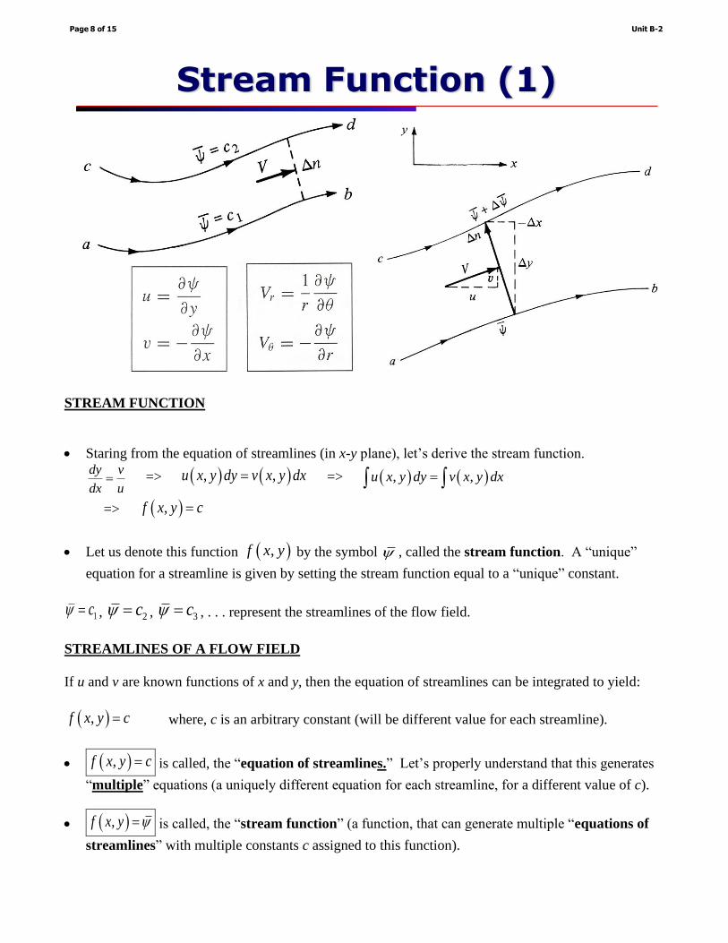
STREAM FUNCTION

• Staring from the equation of streamlines (in x-y plane), let’s derive the stream function. dy v

dx u= => ( ) ( ), ,u x y dy v x y dx= => ( ) ( ), ,u x y dy v x y dx=

=> ( ),f x y c=

• Let us denote this function ( ),f x y by the symbol , called the stream function. A “unique”

equation for a streamline is given by setting the stream function equal to a “unique” constant.

1c = , 2c = , 3c = , . . . represent the streamlines of the flow field.

STREAMLINES OF A FLOW FIELD

If u and v are known functions of x and y, then the equation of streamlines can be integrated to yield:

( ),f x y c= where, c is an arbitrary constant (will be different value for each streamline).

• ( ),f x y c= is called, the “equation of streamlines.” Let’s properly understand that this generates

“multiple” equations (a uniquely different equation for each streamline, for a different value of c).

• ( ),f x y = is called, the “stream function” (a function, that can generate multiple “equations of

streamlines” with multiple constants c assigned to this function).


Stream Function (1)

CONCEPT OF STREAM FUNCTION

Stream function is a mathematical function that can represent a 2-D steady flow field.

For incompressible flow field: = can be defined as the stream function.

• The dimension of stream function is:

kg/(sm): mass flow rate per unit depth.

m3/(sm): volume flow rate per unit depth.

• The difference in stream function represents:

: mass flow (per unit depth) between two adjacent streamlines.

: volume flow (per unit depth) between two adjacent streamlines.


Stream Function (2)

1. = constant gives the equation of a streamline.

2. The stream function can be defined in 2-D flows only.

3. If the stream function is known, the flow field can be described by:

uy

=

vx

= −

1rV

r

=

V

r

= −

VELOCITY POTENTIAL (1)

• Recall that an irrotational flow field is defined as a flow where the vorticity is zero at every point of

the flow field, such that: ( )curl= = =ξ V V 0

• Consider a scalar function , called the velocity potential.

• The vector identity can be written as: ( ) = 0

• This equation states that “for an irrotational flow, there exists a scalar function such that the

velocity is given by the gradient of .”

EQUIPOTENTIAL LINES OF A FLOW FIELD

Similar (in concept) to streamlines, the equation of equipotential lines can be given as:

( ),f x y c= where, c is an arbitrary constant (will be different value for each line).

• ( ),f x y c= is called, the “equation of equipotential lines.” This generates “multiple” equations

(a uniquely different equation for each line, for a different value of c).

• ( ),f x y = is called, the “velocity potential” (a function, that can generate multiple “equations of

equipotential lines” with multiple constants c assigned to this function).

VELOCITY POTENTIAL (2)

The velocity potential is a function of a spatial coordinate: ( , , )x y z = , or ( , , )r z =

For a 3-D Cartesian coordinate system:

ˆ ˆ ˆ ˆˆ ˆu v wx y z

= = + + = + +

V i j k i j k

Therefore: ux

=

, vy

=

, and wz

=


Velocity Potential (1)

CONCEPT OF VELOCITY POTENTIAL

Velocity potential is a mathematical function that can represent a steady irrotational flow field.

If a velocity potential can be defined for a flow field, there will be a significant simplification: Velocity

components ( , , )u v w : 3 unknowns => velocity potential ( ) : 1 unknown

A flow field that can be described by a velocity potential is called, the potential flows.

STREAMLINES AND EQUIPOTENTIAL LINES

Lines of constant : streamlines

Lines of constant : equipotential lines

The slope of a =constant line is the negative reciprocal of the slope of a =constant line: means that

streamlines and equipotential line are mutually perpendicular.

IDEAL (OR POTENTIAL) FLOW FIELD ANALYSIS

• The flow field that can define “velocity potential” (steady and irrotational flow field) is called the

“potential” flow field.

• In aerodynamics I (AE301), we define “ideal” flow field being “incompressible” “potential” flow

field; meaning:

(i) stready,

(ii) no body force,

(iii) inviscid,

(iv) irrotational (because inviscid),

(v) and incompressible.

• Ideal flow field is governed by the equation, called the “Laplace’s equation.”

• “Theoretical aerodynamics” is a basic mathematical analysis, attempting to solve this Laplace’s

equation for an ideal flow field.


Velocity Potential (2)

1. = constant gives the equation of a equipotential lines.

2. The velocity potential can be defined for irrotational flow only.

3. The velocity potential can be defined for both 2-D and 3-D flows.

4. If the velocity potential is known, the flow field can be described by:


Inviscid and Incompressible Flow Equations

Bernoulli’s Equation:

Potential Flow:

Pressure Coefficient:

_________________________________________________________

_________________________________________________________

_________________________________________________________

_________________________________________________________

_________________________________________________________

_________________________________________________________

_________________________________________________________

_________________________________________________________

_________________________________________________________

_________________________________________________________

_________________________________________________________

_________________________________________________________

_________________________________________________________

_________________________________________________________

_________________________________________________________

_________________________________________________________

_________________________________________________________

_________________________________________________________

_________________________________________________________

_________________________________________________________

_________________________________________________________

_________________________________________________________

_________________________________________________________

_________________________________________________________

_________________________________________________________

_________________________________________________________

LAPLACE’S EQUATION (1)

Recall, from the conservation of mass (continuity): ( ) 0t

+ =

V (differential form)

For steady 0t

=

and incompressible ( constant = ) flow, this equation can be simplified to:

0 =V (note: this is the continuity equation of steady & incompressible flow)

(Mathematically, this is the “Divergence of a velocity field”)

LAPLACE’S EQUATION (2)


Laplace’s Equation (1)

_________________________________________________________

_________________________________________________________

_________________________________________________________

_________________________________________________________

_________________________________________________________

_________________________________________________________

_________________________________________________________

_________________________________________________________

_________________________________________________________

_________________________________________________________

_________________________________________________________

_________________________________________________________

_________________________________________________________

_________________________________________________________

_________________________________________________________

_________________________________________________________

_________________________________________________________

_________________________________________________________

_________________________________________________________

_________________________________________________________

_________________________________________________________

_________________________________________________________

_________________________________________________________

POTENTIAL FLOW ANALYSIS

• Potential flow is a flow field that can define a velocity potential.

• Ideal flow field (in aerodynamics I) can be defined as a flow field of steady, inviscid, no body

forces, incompressible, and irrotational.

• The ideal flow is governed by the Laplace’s equation. The ideal flow field can be analyzed by pure

theory (100% mathematical solution), which is essentially “solving the Laplace’s equation” for a

given flow field.

LAPLACE’S EQUATION

• In terms of velocity potential: 3-D Cartesian coordinate system, ( ), ,x y z = :

2 2 22

2 2 20

x y z

= = + + =

• In terms of velocity potential: 3-D cylindrical coordinate system, ( ), ,r z = :

2 22

2 2 2

1 10r

r r r r z

= = + + =

• In terms of stream function: 2-D Cartesian coordinate system, ( ),x y = :

2 22

2 20

x y

= = + =

In 2-D polar coordinate system, ( ),r = :

22

2 2

1 10r

r r r r

= = + =


Laplace’s Equation (2)

Laplace’s equation is:

(1) Partial differential equation (PDE)

(2) with 2nd order

(3) and linear

The Laplace’s equation is a linear 2nd order elliptic PDE. The distinctive features include:

(A) Analytical solutions exist, with a given boundary conditions (called, the “elementary potential flow

solutions”).

(B) These elementary potential flow solutions can be “superimposed” to construct another valid

solution of the flow field.

• Laplace’s equation is the governing equation for an ideal flow field. Therefore, one can analyze

flow field behavior (i.e., velocity, pressure, aerodynamic forces & moments) of an ideal flow field

by “mathematically solve” the Laplace’s equation. This is the very foundation of aerodynamics

(theoretical aerodynamics).

• In AE301, we’ll start with very simple ideal flow field analysis (potential flow theory): flow over a

circular cylinder without and with spin (circulation).

• Hopefully, later, you’ll start using the aerodynamic analysis software (XFOIL / XFLR5). Note that

the software is based entirely on the potential flow theory. Understanding the basic mechanism of

aerodynamic analysis (the potential flow theory) is essentially understanding the theory of

aerodynamics.

• Using the software AS A BLACK BOX is NOT an engineering practice! Anyone can do such a

thing . . . the purpose of AE301 is to understand “how the software works,” and not “using the

software as a black box.”


Class Example Problem B-2-2

Related Subjects . . . “Laplace’s Equation”

Examine Laplace’s equation. What type of equation this is? What are the distinctive

feature(s) of this type of equation?

4 s B- 2: ns Unit B - 2: List of Subjects

Documents

Transcript of 4 s B- 2: ns Unit B - 2: List of Subjects