4 Modeling of Creep in Structures - uni-halle.de · 2006-05-08 · 4 Modeling of Creep in...

4 Modeling of Creep in Structures

In Chapters 2 and 3 we introduced constitutive and evolutionequations for the mod-eling of creep in engineering materials. The objective of Chapt. 4 is the applicationof creep constitutive models to structural analysis. In Sect. 4.1 we start with thediscussion of aims and basic steps in modeling of creep in structures. In Sect. 4.2we formulate initial-boundary value problems describing creep behavior in three-dimensional solids and give an overview on numerical solution procedures. Sections4.3 – 4.4 are devoted to the review and evaluation of structural mechanics models ofbeams, plates and shells in the context of their applicability to the analysis of creepand long term strength. For several problems we develop closed-form solutions andspecial numerical solutions based on the Ritz method. The results are applied to ver-ify finite element solutions obtained by a general purpose finite element code and auser defined material subroutine. Special numerical examples are selected to illus-trate the influence of various discretisation parameters (mesh size, number of Gausspoints, etc.) on the solution accuracy. Furthermore, they allow to compare creep life-time predictions based on different structural mechanics models and related types offinite elements. To discuss the applicability of the developed techniques to real en-gineering problems an example of a spatial steam pipeline ispresented. Long termbehavior of the pipeline under constant internal pressure and constant temperatureis simulated by the finite element method. Numerical resultsare compared with thedata from engineering practice.

4.1 General Remarks

The aim of creep modeling is to reflect basic features of creepin structures includingthe development of inelastic deformations, relaxation andredistribution of stressesas well as the local reduction of material strength (see Sect. 1.2). A model shouldbe able to account for material deterioration processes in order to predict long termstructural behavior and to analyze critical zones of creep failure. Structural analysisunder creep conditions usually requires the following steps:

1. Assumptions must be made with regard to the geometry of thestructure, typesof loading and heating as well as kinematical constraints.

2. A suitable structural mechanics model must be applied based on the assump-tions concerning kinematics of deformations, types of internal forces (mo-ments) and related balance equations.

104 4 Modeling of Creep in Structures

3. A reliable constitutive model must be formulated to reflect time dependentcreep deformations and processes accompanying creep like hardening/recoveryand damage.

4. A mathematical model of the structural behavior (initial-boundary value prob-lem) must be formulated including the material independentequations, consti-tutive (evolution) equations as well as initial and boundary conditions.

5. Numerical solution procedures to solve non-linear initial-boundary value prob-lems must be developed.

6. The verification of the applied models must be performed including the struc-tural mechanics model, the constitutive model, the mathematical model as wellas the numerical methods and algorithms.

The first two steps are common within continuum mechanics andengineering me-chanics. Here, mathematical models of idealized solids andstructures are developedand investigated. Examples include the models of three-dimensional solids, beams,rods, plates and shells. The idealizations are related to the continuum hypothesis,cross section assumptions, etc. The above models were originally developed withinthe theory of linear elasticity, e.g. [126, 308]. In creep mechanics they are appliedtogether with constitutive and evolution equations describing idealized creep behav-ior (e.g. steady state creep) [77, 139, 173, 202, 234]. As mentioned in Sect. 1.1.2and Chapt. 2, many structural materials exhibit non-classical creep phenomena suchas different creep rates under tension and compression, stress state dependence oftertiary creep, damage induced anisotropy, etc. Consideration of such effects mayrequire various extensions of available structural mechanics models. For example,the concept of the stress free (neutral) plane widely used inthe theory of beams andplates becomes invalid in creep mechanics if the material shows different creep ratesunder tension and compression (see Sect. 1.2). Below we discuss the applicabilityof classical and refined models of beams, plates and shells tothe creep analysis.Bases on several examples we examine the accuracy of cross section assumptionsfor displacement and stress fields.

The mathematical model of creep in structure is the initial-boundary value prob-lem (IBVP) which usually includes partial differential equations describing kine-matics of deformation and balance of forces, ordinary differential equations de-scribing creep processes as well as initial and boundary conditions. The numeri-cal solution can be organized as follows, e.g. [77, 250]. Forknown values of thecreep strain tensor and internal state variables at a fixed time the boundary valueproblem (BVP) is solved. Here direct variational methods, e.g. the Ritz method, theGalerkin method, the finite element method are usually applied. In addition, a timestep procedure is required to integrate constitutive and evolution equations of creep.Below various methods are reviewed and discussed with respect to their efficiencyand numerical accuracy.

In recent years the finite element method has become the widely accepted toolfor structural analysis. The advantage of the finite elementmethod is the possibil-ity to model and analyze engineering structures with complex geometries, varioustypes of loadings and boundary conditions. General purposefinite element codes

4.1 General Remarks 105

ABAQUS, ADINA, ANSYS, COSMOS, etc. were developed to solve various prob-lems in solid mechanics. In application to the creep analysis one should take intoaccount that a general purpose constitutive equation whichallows to reflect thewhole set of creep and damage processes in structural materials over a wide rangeof loading and temperature conditions is not available at present. Therefore, a spe-cific constitutive model with selected internal state variables, special types of stressand temperature functions as well as material constants identified from availableexperimental data should be incorporated into the commercial finite element codeby writing a user defined material subroutine. Below the ANSYS finite elementcode is applied to the numerical analysis of creep in structures. In order to considerdamage processes the subroutines “usercreep” and “userout” are developed and im-plemented. The former serves to introduce constitutive equations with damage statevariables and corresponding evolution equations. The latter allows the postprocess-ing of damage, i.e. the creation of contour plots visualizing the damage distributions.

An important question in the creep analysis is that on reliability of the appliedmodels, numerical methods and obtained results. The reliability assessment mayrequire the following verification steps:

– Verification of developed finite element subroutines. To assess that the subrou-tines are correctly coded and implemented, results of finiteelement computa-tions must be compared with reference solutions of benchmark problems. Sev-eral benchmark problems have been proposed in [38] based on an in-house finiteelement code. Below we formulate and solve own benchmark problems includ-ing beams and transversely loaded plates. The advantage of these problems is thepossibility to obtain reference solutions by means of the Ritz method without afinite element discretisation. Furthermore, they allow to verify finite element sub-routines over a wide range of finite element types including beam, shell and solidtype elements.

– Verification of applied numerical methods. Here the problems of the suitable fi-nite element mesh density, the time step size and the time step control must beanalyzed. They are of particular importance in creep damagerelated simulations.Below these problems are discussed based on numerical testsand by means ofcomparison with reference solutions.

– Verification of constitutive and structural mechanics models. This step requirescreep testing of model structural components and the corresponding numericalanalysis by the use of the developed techniques. Examples ofrecent experimen-tal studies of creep in structures include beams [77], transversely loaded plates[163, 224], thin-walled tubes under internal pressure [164, 177], pressure vessels[103, 114], circumferentially notched bars [133]. Let us note that the experimen-tal data for model structures are usually limited to short-term creep tests. Thefinite element codes and subroutines are designed to analyzereal engineeringstructures. Therefore long-term analysis of several typical structures should beperformed and the results should be compared with data collected from engineer-ing practice of power and petrochemical plants. Below an example of the creepfinite element analysis for a spatial steam pipeline is discussed.


4.2 Initial-Boundary Value Problems and GeneralSolution Procedures

The objective of this Section is to discuss the governing mechanical equations de-scribing creep in three-dimensional solids and related numerical solution proce-dures. The set of equations includes material independent equations, constitutiveand evolution equations, see Chapt. 2, as well as the initialand boundary condi-tions. The formulated IBVP must be solved by numerical methods. Explicit andimplicit time integration methods are reviewed with respect to their accuracy andefficiency. Within the time-step procedures, different possibilities are discussed tosolve linearized boundary value problems. The attention will be given to the varia-tional formulations and the use of direct variational methods.

4.2.1 Governing Equations

Let us consider a solid occupying the volumeV with the surfaceA. We assumethat the solid is fixed on the surface partAu and loaded by surface forces on thepart Ap. The position of a material point within the solid in the reference state isdescribed by the position vectorrrr(qi) = eeeiq

i, i = 1, 2, 3, whereeeei are basis vectorsand qi are coordinates (see Sect. A.2.1). The corresponding position in the actualstate can be characterized by the position vectorRRR(qi, t) or by the displacementvectoruuu(qi, t) = RRR(qi, t) − rrr(qi). The problem is to find the time sequence of theactual configurationsRRR(qi, t) as a result of external actions for a given time inter-val and∀qi ∈ V. The governing equations are discussed in continuum mechanicse.g. [29, 35, 44, 57, 108, 131, 178, 199]. Constitutive equations describing creepprocesses have been introduced in Chapt. 2. Besides the kinematical quantities, ad-ditional unknowns are the creep strain tensorεεεcr(qi, t) and the set of internal statevariablesHk(qi, t), k = 1, . . . , n andωl(qi, t), l = 1, . . . , m. They are introducedto characterize the current state of the material microstructure and to reflect the en-tire previous history of the creep process (see Sect. 2.1). In this section we limitour considerations to linearized kinematical equations inthe sense of infinitesimalstrains and displacements. Furthermore, we assume a classical non-polar contin-uum, quasi-static processes and isothermal conditions. The related comments weremade in Sect. 2.1.

The governing equations can be summarized as follows

– kinematical equations• strain-displacement relation

εεε =1

2

(

∇∇∇uuu + (∇∇∇uuu)T)

, qi ∈ V, (4.2.1)

whereεεε is the tensor of infinitesimal strains.• compatibility condition

∇∇∇××× (∇∇∇× εεε)T = 000, qi ∈ V, (4.2.2)

4.2 Initial-Boundary Value Problems and General Solution Procedures 107

– equilibrium conditions

∇∇∇··· σσσ + ρ fff = 000, σσσ× = 000, qi ∈ V, (4.2.3)

whereρ is the material density andfff is the density of volumetric forces– boundary conditions

uuu = uuu, qi ∈ Au,

σσσ ··· ννν = ppp, qi ∈ Ap,(4.2.4)

whereuuu is the given displacement vector andppp is the vector of given surface forcesandννν is the outward unit normal toAp. The vectorsfff , ppp anduuu can be, in general,functions of coordinates and time.

With the assumption of infinitesimal strains the additive decomposition of thetotal strain into elastic, thermal and creep parts is usually postulated

εεε = εεεel + εεεth + εεεcr (4.2.5)

The constitutive equation for the stress tensor can be assumed in the form of thegeneralized Hooke’s law as follows

σσσ = (4)CCC ······ (εεε − εεεth − εεεcr) (4.2.6)

In the case of isotropic elasticity the tensor(4)CCC takes the form

(4)CCC = λIII ⊗ III + µ(eeek ⊗ III ⊗ eeek + eeei ⊗ eeek ⊗ eeei ⊗ eeek), (4.2.7)

whereλ andµ are the Lame’s constants

µ = G =E

2(1 + ν), λ =

νE

(1 + ν)(1 − 2ν)

E is the Young’s modulus,G is the shear modulus,ν is the Poisson’s ratio.If an isotropic solid is heated from the reference temperature T0 up to T, the

thermal part of the strain tensor is

εεεth = αT∆TIII, ∆T ≡ T − T0, (4.2.8)

whereαT is the coefficient of the thermal expansion.∆T can be a function of coor-dinates and time too.

The constitutive equations for the creep rate and evolutionequations for internalstate variables are discussed in Chapt. 2. Here we will use the rate equations in thefollowing form

εεεcr =∂Φ(

σeq(σσσ), Hk, ωl; T)

∂σσσ, k = 1, . . . , n, l = 1, . . . , m,

Hk = Hk

(

σHeq(σσσ), Hk, ωl; T

)

, ωl = ωl

(

σωeq(σσσ), Hk, ωl; T

)(4.2.9)


The hardening variablesHk and the damage variablesωl can be scalars or tensors.For the creep strain as well as for the set of hardening and damage variables theinitial conditions must be specified. Let us assume

εεεcr∣

∣

∣

t=0= 000, Hk

∣

∣

∣

t=0= H0

k , ωl

∣

∣

∣

t=0= ω0

l , (4.2.10)

whereH0k andω0

l are the initial values of the hardening and the damage parameters.Equations (4.2.1) – (4.2.10) describe the quasi-static creep process in a solid.

4.2.2 Vector-Matrix Representation

To formulate initial-boundary value problems and numerical solution procedureslet us rewrite Eqs (4.2.1) – (4.2.10) in the vector-matrix notation. For the sake ofbrevity we introduce the Cartesian coordinatesx1, x2, x3. The Cartesian componentsof vectors and tensors can be collected into the following “numerical” vectors andmatrices:

Stress vector σσσ σσσT = [σ11 σ22 σ33 σ12 σ23 σ31]

Strain vector εεε εεεT = [ε11 ε22 ε33 γ12 γ23 γ31]

Displacement vector uuu uuuT = [u1 u2 u3]

Vector of creep strains εεεcr εεεcrT = [εcr11 εcr

22 εcr33 γcr

12 γcr23 γcr

31]

Vector of internal variables ξξξ ξξξT = [H1 H2 . . . Hn ω1 ω2 . . . ωm]

Vector of thermal strains εεεth εεεthT= [αT∆T αT∆T αT∆T 0 0 0]

Vector of body forces fff fffT

= [ f1 f2 f3]

Vector of surface forces ppp pppT = [p1 p2 p3]

Stress vectorσσσννν onνννdA σσσTννν = [σν1

σν2 σν3 ]

Normal vector ννν νννT = [ν1 ν2 ν3],νi = cos(ννν, xi)


Transformation matrixuuuTTT

uuuTTT =

1 0 00 1 00 0 1

Transformation matrixσσσTTT

σσσTTT =

ν1 0 0 ν2 0 ν3

0 ν2 0 ν1 ν3 00 0 ν3 0 ν2 ν1

Differential matrixDDD

DDD =

∂1 0 0 ∂2 0 ∂3

0 ∂2 0 ∂1 ∂3 00 0 ∂3 0 ∂2 ∂1

Differential matrixDDD1

DDD1 =

0 ∂23 ∂2

2 0 −∂2∂3 0

∂23 0 ∂2

1 0 0 −∂1∂3

∂22 ∂2

1 0 −∂1∂2 0 0

0 0 −∂1∂2 − 12 ∂2

312 ∂1∂3

12 ∂2∂3

−∂2∂3 0 0 12 ∂1∂3 − 1

2 ∂21

12 ∂1∂2

0 −∂1∂3 0 12 ∂2∂3

12 ∂1∂2 − 1

2 ∂22

with

∂i =∂(. . .)

∂xi, ∂2

i =∂2(. . .)

∂x2i

Elasticity matrix (stiffness matrix)EEE

EEE =

(2µ + λ) λ λ 0 0 0(2µ + λ) λ 0 0 0

(2µ + λ) 0 0 0µ 0 0

µ 0SYM µ


Reciprocal elasticity matrix (compliance matrix)EEE−1

EEE−1 =1

E

1 −ν −ν 0 0 01 −ν 0 0 0

1 0 0 02(1 + ν) 0 0

2(1 + ν) 0SYM 2(1 + ν)

With the introduced notations andxxxT = [x1 x2 x3] we can rewrite the governingequations (4.2.1) – (4.2.10) as follows

Kinematical equations:Strain-displacement relation

εεε = DDDTuuu, xxx ∈ V (4.2.11)

Compatibility conditionDDD1εεε = 000, xxx ∈ V (4.2.12)

Prescribed boundary displacementsuuu on Au

uuuTTT uuu = uuu, xxx ∈ Au (4.2.13)

Equilibrium condition:DσDσDσ + fff = 000, xxx ∈ V (4.2.14)

Prescribed surface forcesppp on Ap

σσσTTT σσσ = σσσννν = ppp, xxx ∈ Ap (4.2.15)

Constitutive and evolution equations:

σσσ = EEE(εεε − εεεth − εεεcr), xxx ∈ V (4.2.16)

εεεcr = ggg(σσσ, ξξξ; T)ξξξ = hhh(σσσ, ξξξ; T)

(4.2.17)

Initial conditionsεεεcr(xxx, 0) = 000, ξξξ(xxx, 0) = ξξξ0 (4.2.18)


The functionggg can be formulated if the creep potentialΦ is specified, see Sect.2.1. The vectorξξξ and and the functionhhh can be defined for the selected internalstate variables and the corresponding evolution equations. Examples of hardeningvariables are presented in Sect. 2.3. Damage variables are discussed in Sect. 2.4.

4.2.3 Numerical Solution Techniques

Let us assume that the creep strain vector and the vector of internal state variablesare known functions of the coordinates for a fixed time. With the strain-displacementrelations (4.2.11), the constitutive equations (4.2.16) can be written as follows

σσσ = EEE(DDDTuuu − εεεth − εεεcr) (4.2.19)

Taking into account the equilibrium conditions (4.2.14) and the static boundary con-ditions (4.2.15) we obtain

DDDEEEDDDTuuu = − fff + DDDEEEεεεth + DDDEEEεεεcr, xxx ∈ V,σσσTTT EEEDDDTuuu = ppp+

σσσTTT EEEεεεth+

σσσTTT EEEεεεcr, xxx ∈ Ap

(4.2.20)

With the kinematic boundary conditions (4.2.13), the partial differential equationsand the boundary conditions (4.2.20) represent the BVP withthe displacement vec-tor uuu as an unknown vector. Introducing the fictitious force vectors correspondingto the given thermal strains and the creep strains at fixed time we can write Eqs(4.2.20) as follows

DDDEEEDDDTuuu = − fff + fff th + fff cr, fff th = DDDEEEεεεth, fff cr = DDDEEEεεεcr,σσσTTT EEEDDDTuuu = ppp + pppth + pppcr, pppth =

σσσTTT EEEεεεth, pppcr =

σσσTTT EEEεεεcr

(4.2.21)

These equations are the equilibrium conditions expressed in terms of three unknowncomponents of the displacement vector. After the solution of Eqs (4.2.21) one canobtain the six components of the stress vector from Eq. (4.2.19). Inserting the stressvector into the creep constitutive equations (4.2.17) one can calculate the rates of thecreep strains and those of the internal variables. Based on the equations introduced,the IBVP of the typeYYY = GGG(YYY) can be formulated, whereYYY includes the vectorsof creep strains and internal variables. The operatorGGG involves the solution of thelinearized boundary value problem for the fixed creep strains and internal variables.The initial conditions are Eqs (4.2.18).

An alternative formulation can be based on the compatibility conditions (4.2.12).First the constitutive equations (4.2.16) after differentiation with respect to time canbe written as

σσσ = EEE(εεε − εεεth − εεεcr) = EEE[

εεε − εεεth − ggg(σσσ, ξξξ; T)]

Reordering this equation the total strain vector takes the form

εεε = EEE−1σσσ + εεεth + ggg(σσσ, ξξξ; T) (4.2.22)


For isothermal processesεεεth = 000. The compatibility condition (4.2.12) can berewritten in terms of the strain rate vector

DDD1εεε = 000 (4.2.23)

After inserting (4.2.22) into (4.2.23) we obtain

DDD1EEE−1σσσ + DDD1ggg(σσσ, ξξξ; T) = 000 (4.2.24)

The six equations (4.2.24) describe the stress redistribution during the creep process.The initial conditions are the solutions of the linear elastic problem for the stresses

DDD1EEE−1σσσ(xxx, 0) = 000,

as well asξξξ(xxx, 0) = ξξξ0. The IBVP can be formulated again asYYY = GGG(YYY), whereYYYincludes now the stress vector and the vector of internal state variables. The stressredistribution equation (4.2.24) can be also formulated interms of stress functions.A variety of stress functions can be found in such a way that the equilibrium condi-tions (4.2.14) are identically satisfied. As an example we can introduce the vector ofstress functionsψψψ, so thatσσσ = DDD1ψψψ. It is easy to verify that in the absence of bodyforces the equilibrium conditionsDDDσσσ = DDDDDD1ψψψ = 000 are identically satisfied. Withthe stress functionsψψψ we can write (4.2.24) as follows

DDD1EEE−1DDD1ψψψ + DDD1ggg(DDD1ψψψ, ξξξ; T) = 000

Because there exist identities between the six compatibility conditions (only threeof them are independent), see e.g. [126], it is possible to transform the six equa-tions (4.2.24) into three independent equations. For example, one can express sixcomponents of the stress vector by three Maxwell’s stress functions [126, 253]. Af-ter inserting into (4.2.24) one can obtain three equations for three unknown stressfunctions.

In addition to the displacement formulation (4.2.21) and the stress formulation(4.2.24), it is possible to express the governing equationsin terms of displacementsand stresses. Such mixed formulations can be useful for solving creep problems ofbeams, plates and shells.

4.2.3.1 Time Integration Methods. The governing equations include first or-der time derivatives and the prescribed initial conditions. The unknown displace-ments in Eqs (4.2.21) or the unknown stresses in (4.2.24) arefunctions of coordi-nates and time. The exact integration of these equations with respect to the timevariable is feasible only for one-dimensional problems, e.g. for bars or beams. Inthe general case of the structural analysis, numerical timeintegration methods mustbe applied for solving non-linear IBVP. The commonly used solution technique inmechanics and thermodynamics is the finite difference method. The time derivativesare replaced by finite differences. Starting with the initial conditions (in our case theelastic displacement or stress fields), the finite difference method leads to a step-by-step solution. A variety of time integration algorithms canbe found in textbooks onnumerical methods, e.g. [93, 107, 127, 287].


Here we discuss some typical examples of time integration procedures mostlyused in creep analysis. Let us start with the displacement formulation of the gov-erning equations and neglect the thermal strains for the sake of brevity. The initialcondition is the solution of the elasticity problem

DDDEEEDDDTuuu0 = − fff , σσσ0 = EEEDDDTuuu0 (4.2.25)

with uuu0 = uuu(xxx, 0) andσσσ0 = σσσ(xxx, 0). One way to obtain the displacements andstresses at timet1 = t0 + ∆t1 is to assume that the rates of the creep strains and theinternal state variables are approximately constant within the time interval[t0, t1].Then for any time interval[tn, tn+1] we can write

εεεcrn+1 = εεεcr

n + ∆εεεcrn , ξξξn+1 = ξξξn + ∆ξξξn,

∆εεεcrn = ∆tnggg(σσσn, ξξξn; Tn), ∆ξξξn = ∆tnhhh(σσσn, ξξξn; Tn),

∆tn = tn+1 − tn

(4.2.26)

The displacements and stresses attn+1 can be updated using Eqs (4.2.19) and(4.2.21). Based on the equations introduced we can formulate the following timeintegration scheme:

set n = 0, εεεcr0 = 000, ξξξ0 = 000

solve BVP DDDEEEDDDTuuu0 = − fff , calculate σσσ0 = EEEDDDTuuu0

1: calculate

∆εεεcrn = ∆tnggg(σσσn, ξξξn, Tn), ∆ξξξn = ∆tnhhh(σσσn, ξξξn, Tn)



solve BVP

DDDEEEDDDTuuun+1 = − fff + DDDEEEεεεcrn+1,

σσσn+1 = EEE(DDDTuuun+1 − εεεcrn+1)

(4.2.27)

if tn+1 < tN and ωl < ωl∗, l = 1, . . . , m then set n := n + 1 goto 1

else finish

The calculations can be repeated within the whole given interval of time [t0, tN ]by settingn := n + 1 in Eqs (4.2.26). For the creep-damage related analysis it isnecessary to prove of whether the critical damage state is achieved. If the damagevariable ωl, l = 1, . . . , m attains the critical valueωl∗ the calculations must beterminated.

The forward difference equations (4.2.26) correspond to the one-step explicitEuler method. This method is widely used in the creep analysis because of sim-plicity. The accuracy of the method depends on the time step size. Furthermore,


this method is conditionally stable that means that the stability is restricted to smalltime steps. Therefore stable results can be obtained only for ∆t ≤ ∆tcrit. There isno general recipe how to control the time step size by the use the one step explicitmethod. For example, in [338] it is recommended to compute the time step size fromthe condition that the increment of the creep strain does notexceed one half of theelastic strain, i.e.

∆tnggg(σσσn, ξξξn; Tn) ≤ 1

2EEE−1σσσn

A further restriction is connected with the assumption thatthe stresses have to beconstant within the time interval[tn, tn+1]. Therefore this method can be recom-mended for structural analysis under constant or monotonicloading and tempera-ture conditions only. In the case of loading jumps or cyclic loading changes verysmall time steps are necessary in order to provide a stable solution.

One way to improve the accuracy of time-dependent solutionsis the use ofmulti-step methods of the Runge-Kutta type, see e.g. [77, 107, 127]. These explicitmethods are conditionally stable as well. However, they provide higher order ac-curacy if compared with the one-step forward difference method. Furthermore, forthe creep-damage related analysis the so-called embedded methods [127], which al-low to control the time step size, can be recommended. In [17,18] the embeddedfourth order Kutta-Merson method has been applied to creep problems of shells ofrevolution.

The next possibility to improve the one-step method is the use of the generalizedtrapezoidal rule [93]


n + ∆t[

(1 − θ)εεεcrn + θεεεcr

n+1

]

,

ξξξn+1 = ξξξn + ∆t[

(1 − θ)ξξξn + θξξξn+1

]

,(4.2.28)

whereθ (0 ≤ θ ≤ 1) is the parameter controlling the stability. The rule (4.2.28)includes different well-known methods as special cases. Setting θ = 0 the forwarddifference explicit Euler method (4.2.26) follows. Forθ > 0 we obtain a variety ofimplicit methods: forθ = 1/2 - the trapezoidal rule (Crank-Nicolson method), andfor θ = 1 the backward difference method (implicit Euler method). The advantageof the implicit methods is their unconditional stability that means that the solutionwill be stable independently on the time step size. The pricefor the unconditionalstability is the necessity to solve non-linear equations ateach time step. Equations(4.2.28) can be rewritten as follows


n + ∆εεεcrn ,

ξξξn+1 = ξξξn + ∆ξξξn,

∆εεεcrn = ∆tn [(1 − θ)ggg(σσσn, ξξξn; Tn) + θggg(σσσn+1, ξξξn+1, Tn+1)] ,

∆ξξξn = ∆tn [(1 − θ)hhh(σσσn, ξξξn; Tn) + θhhh(σσσn+1, ξξξn+1, Tn+1)]

(4.2.29)

Equations (4.2.29) are non-linear with respect toξξξn+1 for θ > 0. Note that for amaterial model with strain hardening, the vectorξξξn includes the equivalent creep


strain. In this case Eqs (4.2.29) are non-linear with respect to εεεcrn+1. These equations

can be solved using known iteration methods. The simplest possibility is the fixedpoint iteration method leading to the following scheme at the time step[tn, tn+1]:

set i = 0, εεεcr0

n+1 = εεεcrn , ξξξ i

n = ξξξn, σσσ0n+1 = σσσn

1: calculate

∆εεεcri

n =∆tn

[

(1 − θ)ggg(σσσn, ξξξn; Tn) + θggg(σσσin+1, ξξξ i

n+1; Tn+1)]

,

∆ξξξ in =∆tn

[

(1 − θ)hhh(σσσn, ξξξn; Tn) + θhhh(σσσin+1, ξξξ i

n+1; Tn+1)]

,

εεεcri+1

n+1 = εεεcrn + ∆εεεcri

n , ξξξ i+1n+1 = ξξξn + ∆ξξξ i

n,

if |εεεcri+1

n+1 − εεεcri

n+1| > ǫ and |ξξξ i+1n+1 − ξξξ i

n+1| > ǫ

then solve BVP

DDDEEEDDDTuuui+1n+1 = − fff n+1 + DDDEEEεεεcri+1

n+1 ,

σσσi+1n+1 = EEE

(

DDDTuuui+1n+1 − εεεcri+1

n+1

) (4.2.30)

set i := i + 1 go to 1

else

set εεεcrn+1 = εεεcri+1

n+1 , ξξξn+1 = ξξξ i+1n+1

The accuracy and the efficiency of the implicit method in connection with the in-troduced iteration scheme is now additionally dependent onthe toleranceǫ and theconvergence rate of the fixed point iterations. The first iteration in the above intro-duced scheme is the forward difference predictor. Since theconvergence rate of thefixed point iterations is highly dependent on the “quality” of the first iteration, theefficiency of this scheme is determined again by the time stepsize. If the desired ac-curacyǫ is not reached within3− 4 iterations the time step size should be decreasedand the calculations repeated starting from the step 1. The slow convergence of thefixed point iterations is the drawback of the proposed algorithm. However, in thecase of creep-damage studies this algorithm is more efficient in comparison with theexplicit forward method. Some examples are discussed in [19, 224]. Furthermore,it is possible to combine the implicit time integration scheme with the Newton-Raphson iteration method or its modifications providing higher convergence rates.Examples can be found in [338].

Another widely used technique is to construct an explicit scheme based on thegeneralized trapezoidal rule (4.2.28), see e.g. [36, 247].This can be accomplishedby linearizing (4.2.29 with respect toξξξn+1. For the sake of brevity let us assumethat the functionsggg andhhh are independent fromT. Then we can write

εεεcrn+1

∼= ggg(σσσn, ξξξn) + ggg,σσσ(σσσn, ξξξn)∆σσσn + ggg,ξξξ(σσσn, ξξξn)∆ξξξn,

ξξξn+1∼= hhh(σσσn, ξξξn) + hhh,σσσ(σσσn, ξξξn)∆σσσn + hhh,ξξξ(σσσn, ξξξn)∆ξξξn

(4.2.31)


with

ggg,σσσ =∂ggg

∂σσσ, ggg,ξξξ =

∂ggg

∂ξξξ, hhh,σσσ =

∂hhh

∂σσσ, hhh,ξξξ =

∂hhh

∂ξξξ

From (4.2.29) we obtain

∆εεεcrn = ∆tn

(

gggn + θgggn,σσσ∆σσσn + θgggn,ξξξ ∆ξξξn

)

,

∆ξξξn = ∆tn(

hhhn + θhhhn,σσσ∆σσσn + θhhhn,ξξξ ∆ξξξn)

,(4.2.32)

wheregggn ≡ ggg(σσσn, ξξξn), hhhn ≡ hhh(σσσn, ξξξn),

gggn,σσσ ≡ ∂ggg

∂σσσ(σσσn, ξξξn), gggn,ξξξ ≡ ∂ggg

∂ξξξ(σσσn, ξξξn),

hhhn,σσσ ≡ ∂hhh

∂σσσ(σσσn, ξξξn), hhhn,ξξξ ≡ ∂hhh

∂ξξξ(σσσn, ξξξn)

The second equation (4.2.32) can be rewritten as

∆ξξξn = ∆tn[

III − ∆tnθhhhn,ξξξ

]−1[hhhn + θhhhn,σσσ∆σσσn] (4.2.33)

Inserting this equation into the first equation (4.2.32) we obtain

∆εεεcrn =∆tn(gggn + θgggn,σσσ∆tσσσn)+∆t2

nhhhn,ξξξ

[


]−1[hhhn + θhhhn,σσσ∆σσσn]

(4.2.34)Neglecting the last term in the right-hand side of (4.2.34),the first Eq. in (4.2.20)takes the form

DDDEEEDDDT∆uuun = DDDEEE∆εεεcrn∼= ∆tnDDDEEE [gggn + θgggn,σσσ∆σσσn] (4.2.35)

Here fff = const andεεεth = const are assumed. From (4.2.19) the increment of thestress vector can be computed as follows

∆σσσn = EEE[

DDDT∆uuun − ∆tngggn − ∆tnθgggn,σσσ∆σσσn

]

,

or

∆σσσn = [III + ∆tnθEEEgggn,σσσ]−1 EEEDDDT∆uuun − ∆tn [III + ∆tnθEEEgggn,σσσ]−1 EEEgggn (4.2.36)

After inserting into (4.2.35) we obtain

DDD [EEE − EEE∗n] DDDT∆uuun = ∆tnDDDEEEgggn,

EEE∗n = ∆tnθEEEgggn,σσσ [III + ∆tnθEEEgggn,σσσ]−1 EEE

(4.2.37)

Based on the derived equations it is possible to formulate the following explicitone-step method:


set n = 0, εεεcr0 = 000, ξξξ0 = 000

solve BVP DDDEEEDDDTuuu0 = − fff , calculate σσσ0 = EEEDDDTuuu0

1: calculate

∆εεεcrn =∆tn(gggn + θgggn,σσσ∆tσσσn) ,

∆ξξξn = ∆tn

[


]−1[hhhn + θhhhn,σσσ∆σσσn] ,

EEE∗n = ∆tnθEEEgggn,σσσ [III + ∆tnθEEEgggn,σσσ]−1 EEE

solve BVP

DDD [EEE − EEE∗n] DDDT∆∆∆uuun = ∆tDDDEEEgggn,

∆σσσn = EEE(DDDT∆∆∆uuun − ∆εεεcrn )

(4.2.38)

calculate



uuun+1 = uuun + ∆uuun, σσσn+1 = σσσn + ∆σσσn

if tn+1 < tN and ωl < ωl∗, l = 1, . . . , m

then set n := n + 1 go to 1

else finish

For θ > 0 this method provides an accuracy of higher order if comparedwiththat for the explicit one-step Euler method. For example, for θ = 1/2 the methodhas a second order accuracy while the explicit Euler method (θ = 0) provides afirst order accuracy. Following this algorithm the fictitious force vector∆tDDDEEEgggn

and the stiffness matrixEEE − EEE∗n must be computed at each time step. The modified

stiffness leads to an additional effort in solving the boundary value problem (4.2.38).Furthermore, the matrixEEE − EEE∗

n is non-symmetric.

4.2.3.2 Solution of Boundary Value Problems. According to the discussedtime integration algorithms, linearized boundary value problems have to be solvedat each time or iteration step. These problems include second order partial differen-tial equations with respect to the unknown displacementsuuu(xxx, tn) or displacementincrements∆uuu(xxx, tn). The effect of the accumulated creep strain is considered bymeans of fictitious force vectors and/or complementary stiffness matrices. The accu-mulated creep strain is determined by the entire deformation history. Therefore, theknown analytical methods from the theory of elasticity, e.g. the Fourier series ap-proach [6] and the complex stress functions approach [126],are not applicable in thegeneral case of creep with internal state variables. Only for some one-dimensionalproblems, e.g. for the Bernoulli-Euler type beam, analytical closed form solutionsof the creep problems can be obtained [77, 202, 236]. These solutions are helpful forthe verification of the general computational methods or general purpose solvers.


In what follows let us briefly discuss the numerical methods recently used increep mechanics. These methods are:

– the finite difference method,– the direct variational methods and– the boundary element method.

Applying the finite difference method the partial differential operators are replacedby finite differences leading to the solution of algebraic equations instead of thepartial differential ones. The utilization is mostly efficient for creep problems lead-ing to ordinary differential equations. Examples include axi-symmetrically loadedshells of revolution and circular plates [17, 18, 30, 60, 61,80, 82, 221, 255, 291].

The widely used approach is based on the variational formulations of the creepproblem. Starting from appropriate variational functionals the following direct vari-ational methods can be applied: the Ritz method, the Galerkin method and theVlasov-Kantorovich method. We will briefly discuss the variational formulationsand the classical variational methods in the next subsection. The most powerfulvariational method for the structural analysis is the finiteelement method [37, 338]which is the basis of commercial general purpose solvers, e.g., ABAQUS, ADINA,ANSYS, COSMOS, etc. The possibility to incorporate a creep material model withinternal state variables is available in commercial codes.The implementation can beperformed by writing a user defined material subroutine.

The boundary element method is based on the transformation of the partial dif-ferential equations into boundary integral equations. In order to solve these equa-tions the boundary of the domain is divided into finite elements. As a result a setof algebraic equations with respect to the vector of displacements (tractions) in thediscretisation points of the boundary can be obtained. In the case of creep an ad-ditional domain discretisation is necessary in order to store the components of thecreep strain vector [39]. For details of the boundary element technique we refer to[78, 130, 253].

4.2.3.3 Variational Formulations and Procedures. Variational formulationsare widely used in several problems of solid mechanics. Theyare the basis for directvariational methods, e.g. the Ritz method, the Galerkin method, the finite elementmethod. With respect to the type of the BVP, different variational functionals havebeen proposed. Here let us consider a variational functional in terms of the displace-ment vector. Letuuu(qi, t) be the solution of the BVP (4.2.1) - (4.2.6) under givenεεεcr.Let δuuu be the vector of virtual displacements satisfying the kinematic boundaryconditions (4.2.4). Starting from the equilibrium condition (4.2.3) we can write

∫

V

(∇∇∇ ··· σσσ + ρ fff ) ··· δuuudV = 0 (4.2.39)

According to (A.2.2)∫

V

(∇∇∇ ··· σσσ) ··· δuuudV =∫

V

[

∇∇∇ ··· (σσσ ··· δuuu) − σσσ ······ (∇∇∇δuuu)T]

dV (4.2.40)


Applying the divergence theorem (see Sect. A.2.3) and the static boundary condi-tions (4.2.4) we obtain

∫

V

∇∇∇ ··· (σσσ ··· δuuu)dV =∫

A

(ννν ··· σσσ) ··· δuuudA =∫

Ap

ppp ··· δuuudA (4.2.41)

With σσσ ······ (∇∇∇δuuu)T = σσσ ······ δ(∇∇∇uuu)T = σσσ ······ δεεε, (4.2.40) and (4.2.41), Eq. (4.2.39) takesthe form

∫

V

σσσ ······ δεεεdV −∫

V

ρ fff ··· δuuudV −∫

Ap

ppp ··· δuuudA = 0, (4.2.42)

or

δWi + δWe = 0, δWi = −∫

V

σσσ ······ δεεεdV, δWe =∫

V

f ··· δuuudV +∫

Ap

ppp ··· δuuudA

(4.2.43)The principle of virtual displacements (4.2.43) states that if a deformable systemis in equilibrium then the sum of the virtual work of externalactionsδWe and thevirtual work of internal forcesδWi is equal to zero, e.g., [6, 253, 321]. With theconstitutive equation (4.2.6)

σσσ ······ δεεε =(

(4)CCC ······ (εεε − εεεcr − εεεth))

······ δεεε

=1

2δ(εεε ······ (4)CCC ······ εεε) − (εεεcr + εεεth) ······ (4)CCC ······ δεεε

the variational equation (4.2.43) can be formulated as follows

δ

1

2

∫

V

εεε ······ (4)CCC ······ εεεdV −∫

V

fff ··· uuudV −∫

Ap

ppp ··· uuudA

−∫

V

(εεεcr + εεεth) ······ (4)CCC ······ εεεdV

= 0

or δΠ(uuu) = 0 with

Π(uuu) =1

2

∫

V

εεε ······ (4)CCC ······ εεεdV −∫

V

fff ··· uuudV −∫

Ap

ppp ··· uuudA

−∫

V

(εεεcr + εεεth) ······ (4)CCC ······ εεεdV(4.2.44)

Applying the vector-matrix notation we can write

Π(uuu) =1

2

∫

V

(DDDTuuu)TEEEDDDTuuudV −∫

V

fffT

uuudV −∫

Ap

pppTuuudA

−∫

V

εεεthEEEDDDTuuudV −∫

V

εεεcrEEEDDDTuuudV(4.2.45)


It is easy to verify that from the conditionδΠ(uuu) = 0 follows the partial differentialequation with respect to the displacement vector and the static boundary condition(4.2.20).

The variational functional (4.2.45) has been derived from the principle of vir-tual displacements. By analogy a variational functional interms of stresses or stressfunctions can be formulated providing Eqs (4.2.24) as Eulerequations. Furthermore,a mixed variational formulation in terms of displacements and stresses can be conve-nient for numerous structural mechanics problems. In [18, 224] a mixed variationalfunctional has been utilized for the solution of the von Karman type plate equations.In [16, 20, 225] a mixed formulation has been applied to derive the first order sheardeformation beam equations.

To solve the variational problem classical direct variational methods can be uti-lized. Let us illustrate the application of the Ritz method to the variational functional(4.2.45). The approximate solution for the displacement vector uuu is presented in theform of series

uk =N

∑i=1

akiφki(x1, x2, x3), k = 1, 2, 3 (4.2.46)

(no summation overk) or

uuu ≡

u1

u2

u3

=

aaaT1 φφφ1

aaaT2 φφφ2

aaaT3 φφφ3

=

φφφ1 000 000

000 φφφ2 000

000 000 φφφ3

T

aaa1

aaa2

aaa3

= GGGTaaa, (4.2.47)

whereφφφk are vectors of the trial (basis or shape) functions which should be speci-fied a priori andaaak are vectors of unknown (free) parameters. The functionsφki in(4.2.46) must be linearly independent and satisfy the kinematical boundary condi-tions. Furthermore, the set of these functions must be complete in order to providethe convergence ofuuu as N → ∞. Inserting the approximate solutionuuu into thevariational functional (4.2.45) we can obtain for the time step tn

Πn(uuu) = aaaT

1

2

∫

V

(DDDTGGG)TEEEDDDTGGGdV

aaa − aaaT∫

V

GGGfff dV − aaaT∫

Ap

GGGpppdA

− aaaT

∫

V

(DDDTGGG)TEEEεεεthTdV +

∫

V

(DDDTGGG)TEEEεεεcrn

TdV

=1

2aaaTKKKaaa − aaaT( fff + fff th + fff cr

n ) = Πn(aaa)

(4.2.48)with


KKK =∫

V

(DDDTGGG)TEEEDDDTGGGdV =∫

V

BBBTEEEBBBdV, BBB = DDDTGGG,

fff =∫

V

GGGfff dV −∫

Ap

GGGpppdA,

fff th =∫

V

BBBTEEEεεεthTdV, fff cr

n =∫

V

BBBTEEEεεεcrn

TdV

From the conditionδΠn(aaa) = 0 follows the set of linear algebraic equations

KKKaaa = fff + fff th + fff crn (4.2.49)

After the solution of (4.2.49) the displacements can be computed from (4.2.47) andstresses from (4.2.19). With the Ritz method and the explicit time integration pro-cedure the step-by-step solution of a creep problem can be utilized as follows:

set n = 0, εεεcr0 = 000, ξξξ0 = 000

select the matrix of trial functions GGG

calculate

KKK =∫

V

BBBTEEEBBBdV, fff =∫

V

GGGfff dV −∫

Ap

GGGpppdA, fff th =∫

V

(DDDTGGG)TEEEεεεthTdV

solve BVP KKKaaa0 = fff + fff th calculate uuu0 = GGGTaaa0, σσσ0 = EEEDDDTuuu0

1: calculate

∆εεεcrn = ∆tnggg(σσσn, ξξξn, Tn), ∆ξξξn = ∆tnhhh(σσσn, ξξξn, Tn)



calculate

fff crn+1 =

∫

V

(DDDTGGG)TEEEεεεcrn+1

TdV

solve KKKaaan+1 = fff + fff th + fff crn+1

calculate uuun+1 = GGGTaaan+1, σσσn+1 = EEE(DDDTuuun+1 − εεεcrn+1)

if tn+1 < tN and ωl < ωl∗, l = 1, . . . , m

then set n := n + 1 go to 1

else finish

The vectorfff crn must be computed at each time step through a numerical integration.

Therefore, the domain discretisation is required to store the vectorsεεεcr andξξξ. Theaccuracy of the solution by the Ritz method depends on the “quality” and the num-ber of trial functions. For special problems with simple geometry, homogeneous


boundary conditions, etc., trial functions can be formulated in terms of elemen-tary functions (e.g. orthogonal polynomials, trigonometric or hyperbolic functionsetc.) defined within the whole domain, e.g. [6]. Examples forsuch problems includebeams [14, 77, 225] and plates [18, 224]. The Ritz method is simple in utilizationand provides an approximate analytical solution.

In the general case of complex geometry, a powerful tool is the finite elementmethod. The domain is subdivided into finite elements and thepiecewise trial func-tions (polynomials) are defined within the elements. For details of finite elementtechniques we refer to the textbooks [37, 56, 325, 338]. By analogy with the Ritzmethod the finite element procedure results in a set of algebraic equations of thetype

KKKδδδn = fff + fff th + fff crn , (4.2.50)

whereKKK is the overall stiffness matrix,δδδn is the vector of unknown nodal displace-ments andfff , fff th and fff cr

n are the nodal force vectors computed from given loads,thermal strains as well as creep strains at the time or iteration step. The commercialcodes usually include more sophisticated time integrationmethods allowing the au-tomatic time step size control. The vectorfff cr

n depends on the distribution of creepstrains at the current time step. The creep strains are determined by the constitutivemodel and a variety of constitutive models can be applied depending on the materialtype, type of loading, available experimental data, etc. Therefore the possibility toincorporate a user defined material law is usually availablein commercial codes.

4.3 Beams 123

4.3 Beams

Beams are widely discussed in monographs and textbooks on creep mechanics[77, 139, 152, 173, 201, 202, 234, 250, 292]. The presented examples are, how-ever, limited to the classical Bernoulli-Euler beam theoryand Norton-Bailey con-stitutive equations of steady state creep. The objective ofthis section is to analyzetime dependent behavior of beams under creep-damage conditions. For this purposewe apply the classical beam theory and a refined theory which includes the effectof transverse shear deformation (Timoshenko type theory).Based on several exam-ples we compare both theories as they describe creep-damageprocesses in beams.Furthermore, we develop and solve several benchmark problems. The reference so-lutions obtained by the Ritz method are applied to verify user-defined creep-damagematerial subroutines for the ANSYS finite element code.

4.3.1 Classical Beam Theory

4.3.1.1 Governing Equations. Let us consider a straight homogeneous beam inthe Cartesian coordinate systemx, y, z as shown in Fig. 4.1. For the sake of brevitywe consider the case of symmetrical bending in the plane spanned on thex andz coordinate lines. Furthermore we introduce geometricallylinear equations. Theirvalidity is restricted to the case of infinitesimal strains,displacements and crosssection rotations. The governing equations can be summarized as follows

– kinematical equations

eeex

eeex

eeez

eeez

eeey

eeey

x

q(x)eeez

z

P

Prrr

rrrtCentroid of cross section

rrr(x, y, z) = eeexx + rrrt(y, z)

rrrt(y, z) = eeeyy + eeezz

Figure 4.1 Beam with a rectangular cross section. Geometry, loading and coordinates


u(x, z) = u0(x) + ϕ(x)z, ϕ(x) = −w′(x),

εx(x, z) = u′0(x) + ϕ′(x)z,

(4.3.1)

whereu(x, z) is the axial displacement,u0(x) is the axial displacement of thebeam centerline,ϕ(x) is the angle of the cross section rotation,w(x) is the trans-verse displacement (deflection) and prime denotes the derivative with respect tox.


N′(x) = 0, Q′(x) + q(x) = 0, M′(x) = Q(x), (4.3.2)

whereN(x) is the normal force,Q(x) is the shear force,M(x) is the bendingmoment andq(x) is the given distributed load.

– constitutive equations• normal (bending) stress

σx(x, z) = E[εx(x, z) − αT∆T(x, z) − εcrx (x, z)]

= E[ε0(x) + χ(x)z − αT(x, z)∆T − εcrx (x, z)],

(4.3.3)

whereε0 = u′0 is the strain of the beam centerline andχ = −w′′ is the beam

curvature.• stress resultants

N(x) =∫

A

σxdA = EA[

ε0(x) − εcr0 (x) − εth

0 (x)]

,

M(x) =∫

A

σxzdA = EI[

χ(x)− χcr(x) − χth(x)]

,(4.3.4)

whereA is the cross sectional area,I is the moment of inertia and

εcr0 (x) =

1

A

∫

A

εcrx (x, z)dA, εth

0 (x) = αT1

A

∫

A

∆T(x, z)dA,

χcr(x) =1

I

∫

A

εcrx (x, z)zdA, χth(x) = αT

1

I

∫

A

∆T(x, z)zdA

are averages of thermal and creep strains. In terms of fictitious forces and mo-ments Eqs (4.3.4) can be rewritten as follows

N(x) = EAε0(x) − Ncr(x) − Nth(x),

M(x) = EIχ(x)− Mcr(x) − Mth(x)(4.3.5)

with

Ncr(x) = E∫

A

εcrx (x, z)dA, Nth(x) = EαT

∫

A

∆T(x, z)dA,

Mcr(x) = E∫

A

εcrx (x, z)zdA, Mth(x) = EαT

∫

A

∆T(x, z)zdA,

4.3 Beams 125

• creep-damage constitutive and evolution equations (see Sect. 2.4.1.1)

εcrx =

a|σx |n−1σx

(1 − ω)n, ω =

bσkeq

(1 − ω)l, σeq = α

|σx | + σx

2+ (1 − α)|σx |

(4.3.6)

The boundary conditions atx = 0 andx = l (l is the beam length) must be formu-lated with respect to the kinematical quantitiesw, ϕ and/or the dual static quantitiesQ, M. The initial conditions att = 0 areεcr

x = 0 andω = 0.

4.3.1.2 Closed Form Solutions. Assuming the idealized creep behavior withthe secondary creep stage only (see Sect. 1.2) a steady stateexists, for which thebending stress and the deflection rate in a beam are constant.Constitutive equationfor secondary creep follows from (4.3.6) by settingb = 0. For the sake of brevitylet us neglect the thermal strains. The constitutive equation for the bending stress(4.3.5) takes the form

σx(x, z) = E [χ(x)z − εcrx (x, z)] (4.3.7)

In the following derivations let us drop the arguments. Taking the time derivative of(4.3.7) and applying the constitutive equation (4.3.6) we obtain

σx = E(χz − a|σx |n−1σx) (4.3.8)

Equation (4.3.8) describes the stress redistribution in a beam. The steady state solu-tion follows from (4.3.8) by settingσx = 0

σx =

(

1

a

) 1n

|χz| 1n −1χz (4.3.9)

The bending moment in the steady state can be calculated as follows

M =∫

A

σxzdA =

(

1

a

) 1n

In|χ|1n −1χ, (4.3.10)

whereIn =

∫

A

|z| 1n−1z2dA

is the generalized moment of inertia.As an example let us consider a simply supported beam under a uniformly dis-

tributed loadq. In this statically determined case the bending moment isM(x) =qx(l − x)/2. From (4.3.10) follows the differential equation for the deflection rate

w(x)′′ = − a

Inn

qn

2nxn(l − x)n, 0 ≤ x ≤ l (4.3.11)

For integer values of the powern the solution is


w(x) =a

Inn

qn

2nx

n

∑k=0

αk(ln+k+1 − xn+k+1) (4.3.12)

with

αk = (−1)k n!

k!(n − k)!

ln−k

(n + k + 1)(n + k + 2)

The reference elastic deflection is

w(x) =q

24EIx(x − l)(x2 − lx − l2)

Let us note that the closed form solution for the steady statedeflection rate (4.3.12)is a polynomial of the order2n + 2. Therefore, if the creep problem is numericallysolved applying variational methods (see Sect. 4.2.3.3), the trial functions for the de-flection or deflection rate should contain the polynomial terms of the order2n + 2instead of 4 in the elastic case. The order of the polynomial terms of the creep solu-tion is material-dependent sincen is the creep exponent in the Norton-Bailey creeplaw. Furthermore, for the analysis of steady state creep, anaccurate solution cannotbe obtained applying approximations justified from the elastic solution. Closed formsolutions for steady state creep in beams with various typesof boundary conditionsand loading are presented in [77, 202, 234].

4.3.1.3 Approximate Solutions by the Ritz Method. Starting from the prin-ciple of virtual displacements (4.2.43) we can write

∫

V

σxδεxdV = EI

l∫

0

w′′δw′′dx + EA

l∫

0

u′0δu′

0dx

+

l∫

0

Mcrδw′′dx −l∫

0

Ncrδu′0dx

=

l∫

0

qδwdx

Assuming the creep strain to be known function of the coordinatesx andz for thefixed timet we can formulate the following functional

Πt(w, u0) =1

2EI

l∫

0

w′′2dx +1

2EA

l∫

0

u′20 dx

+

l∫

0

Mcrw′′dx −l∫

0

Ncru′0dx −

l∫

0

qwdx

The problem is to find such functionsw andu0 that yield an extremum of the func-tional. The approximate solutions for the fixed timet can be represented in the formof series

4.3 Beams 127

w(x) = aw0 φw

0 (x) +N

∑i=1

awi φw

i (x), u0(x) =M

∑i=1

aui φu

i (x) (4.3.13)

For the simply supported beam the trial functions can be formulated as follows.φw

0 (x) = x(x− l)(x2 − lx− l2) is the first approximation from the elastic solution.For φw

i (x) we apply the following polynomials satisfying the boundaryconditionsfor the deflectionw = 0 and for the bending momentM = 0 at x = 0 andx = l

φωi (x) = xi+2(l − x)i+2 (4.3.14)

Assuming thatu0 = 0 atx = 0 the functionsφui (x) = xi can be utilized. Collecting

the unknown constant coefficients into the vectoraaaT = [aaawTaaauT

] with aaawT=

[aw0 aw

i ], i = 1, . . . , N andaaauT= [au

i ], i = 1, . . . , M, the Ritz method yields a setof linear algebraic equations

∂Πt

∂ak= 0,

[

RRRww 000000 RRRuu

] [

aaaw

aaau

]

=

[

fff w

fff u

]

(4.3.15)

with

Rwwkj = EI

l∫

0

φwk′′φw

j′′dx, k = 1, . . . , N, j = 1, . . . , N,

Ruukj = EA

l∫

0

φuk′φu

j′dx, k = 1, . . . , M, j = 1, . . . , M,

f wk = q

l∫

0

φwk dx −

l∫

0

Mcrφwk′′dx, k = 1, . . . , N,

f uk =

l∫

0

Ncrφuk′dx, k = 1, . . . , M

After solution of (4.3.15) the stressσx(x, z, t) can be calculated from (4.3.3). Forthe known values of the stress and the damage parameter the constitutive model(4.3.6) yields the rates of creep strain and damage for the time t. From these thenew values for the timet + ∆t are calculated using the implicit time integrationprocedure (4.2.28)

εcr(x, z, t + ∆t) = εcr(x, z, t) + ∆t[(1 − θ)εcr(x, z, t) + θεcr(x, z, t + ∆t)],

ω(x, z, t + ∆t) = ω(x, z, t) + ∆t[(1 − θ)ω(x, z, t) + θω(x, z, t + ∆t)],

εcr(x, z, 0) = 0, ω(x, z, 0) = 0, ω(x, z, t) < ω∗

For the calculation of the fictitious creep forceNcr and the creep momentMcr

the Gauss method with 9 integration points in the thickness direction is used. To


obtain the matricesRRRmn(m, n = w, u) and the vectorsfff w and fff u in (4.3.15) theSimpson quadrature rule withNs integration points along the beam length axisx isapplied. The values of creep strain and damage at the currenttime step are storedfor all integration points along the beam axis and over the thickness direction. Theyare used for the calculations at the next time step. The accuracy of the numericalsolution depends on the number of trial functions in Eq. (4.3.13), on the number ofintegration points, and on the time step size.

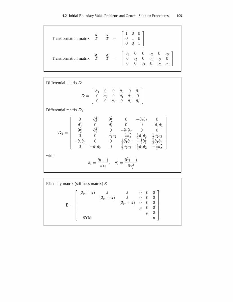
4.3.1.4 Example. In the following numerical example we examine the conver-gence of the approximate solution by the Ritz method applying different numberof trial functions. Furthermore, we perform the finite element analysis by ANSYScode to verify the developed material subroutine and to illustrate the solution accu-racy with respect to the mesh density.

Solution by the Ritz Method. Let us consider a simply supported and uniformlyloaded beam with a rectangular cross sectiong× h, whereg is the width andh is theheight. For the numerical analysis we setq = 60 N/mm, l = 103 mm,h = 80 mm,ly = 30 mm. We apply the creep-damage material model (3.1.11) with materialconstants for the aluminium alloy BS 1472 (3.1.12) (see Sect. 3.1.4). The damageevolution is controlled by the von Mises equivalent stress.Consequently, the damagerate will be the same for tensile and compressive layers of the beam. By settingα = 0 in (4.3.6) we obtainσeq = |σx |. Therefore, the distribution of|σx | willbe symmetrical with respect to the beam centerline. Furthermore, in Eqs (4.3.15)Ncr = 0, fff u = 000 and consequentlyaaau = 0.

The time step solutions are performed until the critical damage is achieved inone of the integration points. The condition of terminationis ω(x f , z f , t∗) > 0.9,where the integration pointP(x f , z f ) can be specified as a point of failure initia-tion and the time stept∗ as the time to failure initiation. Figure 4.2 illustrates themaximum deflection and the maximum stress as functions of time. The results havebeen obtained with different number of polynomial terms (4.3.14) in Eqs (4.3.13).We observe that all applied approximations to the deflectionfunction provide thesame result for the reference elastic state. However, the results for creep are quitedifferent and depend essentially on the number of trial functions, Fig. 4.2. The ap-proximation adjusted to the elastic solution (fourth orderpolynomial, curves 1) ishardly sufficient for the creep-damage analysis. The difference between the life-timeestimations for the case 1 (N = 1) and for the case 4 (N = 8) is up to the factor six.Figure 4.3 illustrates the convergence against the accurate solution with increasingnumber of trial functions. As shown in Sect. 4.3.1.2, the closed form solution fordeflection rate in the steady state creep range is a polynomial of the order2n + 2,wheren is the material constant in the power law. If the damage evolution is takeninto account then the steady state creep range does not exist, Fig. 4.3. By analogywith the uni-axial creep curve three creep stages for the beam can be observed. The“primary” stage is characterized by the decrease in the deflection rate and signifi-cant stress relaxation. The “secondary” stage can be identified by slow changes inthe rates of deflection growth and stress relaxation. Duringthe “tertiary” stage therates rapidly increase. The applied approximations in the cases 3-6, Fig. 4.3, provide

4.3 Beams 129

0 5 0 0 0 0 1 0 0 0 0 0 1 5 0 0 0 0 2 0 0 0 0 0 2 5 0 0 0 08

1 0

1 2

1 4

1 6

1 8

2 0

2 2

0 5 0 0 0 0 1 0 0 0 0 0 1 5 0 0 0 0 2 0 0 0 0 0 2 5 0 0 0 08 0

1 0 0

1 2 0

1 4 0

1 6 0

1 8 0

2 0 0

2 2 0

2 4 0

t, h

t, h

wmax, mm

σmax = σx(l/2, h/2), MPa

1

1

2

2

3

3

4

4

q

lP(l/2, h/2)wmax

a

b

Figure 4.2 Solutions for a Bernoulli beam based on the Ritz method with the approximation(4.3.13) and polynomial functions (4.3.14).a Time variation of maximum deflection,b timevariation of maximum stress, 1 – approximation using elastic deflection function, 2 –N = 1,3 – N = 2, 4 – N = 8

almost the same solutions for the primary and secondary creep stages. The resultsdiffer only in the final stage. Therefore we may conclude thatthe consideration ofdamage needs an increased order of approximation, in comparison with the steadystate creep analysis.

Finite Element Solution. The constitutive model (3.1.3) is incorporated into theANSYS finite element code by means of the user defined creep material subrou-


0 1 0 0 0 0 2 0 0 0 0 3 0 0 0 0 4 0 0 0 0 5 0 0 0 0 6 0 0 0 08

1 0

1 2

1 4

1 6

1 8

2 0

2 2

0 1 0 0 0 0 2 0 0 0 0 3 0 0 0 0 4 0 0 0 0 5 0 0 0 0 6 0 0 0 08 0

1 0 0

1 2 0

1 4 0

1 6 0

1 8 0

2 0 0

2 2 0

2 4 0

t, h

t, h

wmax, mm

σmax, MPa

1

1

2

2

3

3

4

4

5

5

6

6

a

b

Figure 4.3 Convergence of time-dependent solution for a Bernoulli beam using polynomialfunctions (4.3.14).a Time variation of maximum deflection,b time variation of maximumstress, 1 –N = 1, 2 – N = 2, 3 – N = 3, 4 – N = 5, 5 – N = 7, 6 – N = 8

tine. For details of the ANSYS User Programmable Features and the utilized timeintegration methods we refer to [258, 338].

To verify the developed subroutine and to analyze the accuracy of finite elementsolutions with respect to the mesh density, the type of finiteelements, the type ofthe time integration procedure, etc., benchmark problems are required. Here weconsider the example solved before by the Ritz method. For the meshing we used

4.3 Beams 131

0 1 0 0 0 0 2 0 0 0 0 3 0 0 0 0 4 0 0 0 0 5 0 0 0 0 6 0 0 0 08

1 0

1 2

1 4

1 6

1 8

2 0

2 2

0 1 0 0 0 0 2 0 0 0 0 3 0 0 0 0 4 0 0 0 0 5 0 0 0 0 6 0 0 0 08 0

1 0 0

1 2 0

1 4 0

1 6 0

1 8 0

2 0 0

2 2 0

2 4 0

t, h

t, h

wmax, mm

σmax, MPa

1

1

2

2

3

3

4

4

5

5

6

6

q = q/g

a

b

Figure 4.4 Solutions for a Bernoulli beam using the ANSYS code with elements SHELL 43.a Time variation of maximum deflection,b time variation of maximum stress, 1 – 8 elements,2 – 10 elements, 3 – 20 elements, 4 – 40 elements, 5 – 80 elements, 6 – 200 elements

the 4-node shell element SHELL 43 available in ANSYS for creep and plasticityanalysis. For the time integration we applied the automatical time stepping featurewith a minimum time step0.1 h.

Figure 4.4 illustrates time variations for the maximum defection and the max-imum stress. The results have been obtained with a differentnumber of elementsalong the beam axis. We observe that all of the used meshes provide the same solu-


tions for the reference elastic state. However, the creep solutions are highly sensitiveto the mesh density. The best solution (case 6) has been obtained with 200 elementsand after 96 time steps. This solution agrees well with the solution obtained by theRitz method, Fig. 4.3. A mesh adjusted to the convergent solution of the linear elas-ticity problem (case 1) is not fine enough for the creep analysis. The results in thecases 3-6, Fig. 4.4 agree well in the primary and secondary creep stages and dif-fer only in the final stage. However, such a difference is not essential if we takeinto account the scatter of material data and inaccuracy of the material behavior de-scription. In this sence the mesh adjusted to the convergentsolution in the pimaryand secondary creep stages is fine enough for the numerical life-time predictions.In [14, 15] several benchmark problems for beams and rectangular plates solved bythe Ritz method are presented. Finite element solutions forthe same problems havebeen perfomed by use of shell, plane and solid type elements.The results illustratethe correctness of the developed subroutine over the wide range of element types.Furthermore, the conclusion was made, that the mesh adjusted to convergent solu-tions in the primary and secondary creep range provides enough accuracy for theanalysis of the whole creep process.

4.3.2 Refined Theories of Beams

4.3.2.1 Stress State Effects and Cross Section Assumptions . For manymaterials stress state dependent tertiary creep has been observed in multi-axial tests(see Sect. 1.1.2). The primary and secondary creep rates aredominantly controlledby the von Mises stress. The accelerated creep is additionally influenced by the kindof the stress state. For example, different tertiary creep rates and times to fracturecan be obtained from creep tests under uni-axial tension with the stressσ and undertorsion with the shear stress

√3τ = σ, e.g. [169]. Figure 4.5a shows creep curves

for tensile, compressive and shearing stresses simulated according to the constitutivemodel (3.1.1), (3.1.2) and the material constants (3.1.3) for type 316 stainless steelat 650 C. The selected stress values provide the same value of the von Mises stress.It is obvious that the tertiary creep rate is significantly dependent on the kind ofloading. Figure 4.5b presents creep curves calculated by the combined action of thenormal and shear stresses. We observe that even a small superposed shear stress cansignificantly influence the axial strain response and decrease the fracture time. Fur-thermore, combined tension-shear and compression-shear loadings with the samestress magnitudes lead to quite different creep responses.The change of the sign ofthe normal stress influences both the normal and the shear creep rates.

The considered loading case is typical for transversely loaded beams, plates andshells. For beams the local stress state is characterized bynormal (bending) stressand small superposed transverse shear stress. Transverse shear stress and transverseshear deformation are neglected within the classical theory of beams. The consid-ered example indicates that small shear stress can significantly influence the ma-terial response and cause significant shear strains. Furthermore, the dependence ofcreep on the sign of the normal stress can lead to non-classical thickness distribu-tions of the displacement, strain and stress fields. For example, the concept of the

4.3 Beams 133

0 1 0 0 0 2 0 0 0 3 0 0 0 4 0 0 0 5 0 0 0 6 0 0 0 7 0 0 0 8 0 0 0 9 0 0 0 1 0 0 0 00

0 . 0 0 0 5

0 . 0 0 1

0 . 0 0 1 5

0 . 0 0 2

0 . 0 0 2 5

0 . 0 0 3

0 1 0 0 0 2 0 0 0 3 0 0 0 4 0 0 0 5 0 0 0 6 0 0 0 7 0 0 00

0 . 0 0 0 5

0 . 0 0 1

0 . 0 0 1 5

0 . 0 0 2

0 . 0 0 2 5

0 . 0 0 3

0 . 0 0 3 5

t, h

t, h

εcr, γcr/√

3

εcr, γcr/√

3

σ = 50 MPa

τ = 28.5 MPa

σ = −50 MPa

σ = 50MPaτ = 15MPa

σ = 50 MPa

σ = −50MPaτ = 15MPa

εcrεcr

εcr

γcr/√

3

γcr/√

3

γcr/√

3

|εcr|

|εcr|

a

b

Figure 4.5 Creep responses for various stress states computed using Eqs (3.1.1) – (3.1.3).a Responses by tension, torsion and compression,b responses by combined tension (com-pression) and torsion

neutral stress-free plane fails and the distribution of thetransverse shear stresses isnon-symmetrical with respect to the midplane.

Cross section assumptions are usually the basis for different refined models ofbeams, plates and shells developed within the theory of elasticity. Below we applythe first order shear deformation theory (Timoshenko-type theory) to creep analysis.For a beam with a rectangular cross section we compare the results based on differ-


ent structural mechanics models (classical beam, shear deformable beam and planestress model).

4.3.2.2 First Order Shear Deformation Equations. The first order shear de-formation beam theory can be derived either by the direct approach, e.g. [32], or bya variational method applied to three-dimensional equations, e.g. [20, 140].

Within the direct approach the beam is modeled as a deformable oriented line.The deformed configuration is characterized by two independent kinematical quan-tities: the vector describing the positions of points on theline and the rotation tensoror vector describing the orientation of cross sections. Furthermore, it is assumed thatthe mechanical interaction between neighboring cross sections is only due to forcesand moments. The balance equations are applied directly to the deformable lineand formulated with respect to the beam quantities, i.e. theline mass density (massdensity per unit arc length), the vectors of forces and moments, the line densityof internal energy, etc. The constitutive equations connect the forces and momentswith the strains. A direct approach to formulate constitutive equations for rods andshells in the case of elasticity is discussed in [23]. Despite the elegance of this ap-proach several problems arise in application to creep mechanics. The creep consti-tutive equations must be formulated for inelastic parts of beam like strains (tensile,transverse shear and bending strains). By analogy to the creep theories discussed inChapt. 2 the creep potential should be constructed as a function of the force and themoment vectors. For example, letTTT be the force vector andMMM the moment vector.Following the classical creep theory (see Sect. 2.2.1.1) anequivalent stress for thedeformable line can be formulated as a quadratic form with respect toTTT andMMM

t2eq =

1

2TTT ··· AAA ··· TTT + TTT ··· BBB ··· MMM +

1

2MMM ···CCC ··· MMM

The structure of second rank material tensorsAAA, BBB andCCC must be established ac-cording to the material symmetries and geometrical symmetries of the beam crosssection. The material constants have to be identified eitherfrom creep tests on beamsor by comparing the solutions of beam equations with the corresponding solutionsof three- or two-dimensional problems for special cases of loading. Only a few suchsolutions are available in creep mechanics. An example is the pure bending of abeam under power law secondary creep condition (see Sect. 4.3.1.2). In this casethe steady state creep constitutive equation for the bending strain rate can be ob-tained from (4.3.10) as follows

χ =a

Inn|M|n−1 M

Alternatively the beam equations may be derived in the senseof approximate so-lution of two- or three-dimensional equations. First, through-the-thickness approx-imations of displacements and/or stresses are specified. Then, the two- or three-dimensional boundary value problem is reduced to ordinary differential equationsby means of a variational principle. In order to discuss thisapproach let us considera beam with a rectangular cross-section, Fig. 4.6. The governing two-dimensional

4.3 Beams 135

x

z z

y

h/2

h/2

g

q(x)

Figure 4.6 Straight beam with a rectangular cross-section

equations for this case can be derived from (4.2.1) - (4.2.9)under the assumption ofthe plane stress state, i.e.σσσ ··· eeey = 000. The principle of virtual displacements (4.2.43)yields

gh

2

l∫

0

1∫

−1

(σxδεx + τxzδγxz + σzδεz)dζdx =

l∫

0

q(x)δw(x,−h/2)dx (4.3.16)

Here l denotes the beam length,σx, σy, τxz and εx, εy, γxz are the Cartesian com-ponents of the stress and strain tensors, respectively,w is the beam deflection andζ = 2z/h is the dimensionless thickness coordinate. Here and in the followingderivations we use the abbreviations

(. . .),x ≡ ∂

∂x(. . .), (. . .),z ≡

∂

∂z(. . .), (. . .)′ ≡ d

dx(. . .),

(. . .)• ≡ d

dζ(. . .), ˙(. . .) ≡ d

dt(. . .)

Specifying through-the-thickness approximations for theaxial displacementuand the deflectionw, various one-dimensional displacement based beam theoriescan be derived [268]. The classical Bernoulli-Euler theoryis based on the followingdisplacement approximations

u(x, z) = u0(x) − w′0(x)

h

2ζ, w(x, z) = w0(x), (4.3.17)

whereu0, w0 are the displacements of the beam centerline. The refined assumption

u(x, z) = u0(x) + ϕ(x)h

2ζ, (4.3.18)

where ϕ denotes the independent cross-section rotation, providesthe first ordershear deformation (Timoshenko-type) beam theory. Anotherrefined displacementbased beam model can be obtained with


u(x, ζ) = u0(x) + ϕ(x)h

2ζ + u1(x)Φ(ζ),

w(x, ζ) = w0(x) + w1(x)Ω(ζ),(4.3.19)

whereu0 and w0 are the displacements of the beam centerline,Φ(ζ) and Ω(ζ)are distribution functions, which should be specified, andu1(x) andw1(x) are un-known functions of thex-coordinate. The assumptionsΦ(ζ) = (ζh/2)3 , Ω(z) = 0result in a Levinson-Reddy type theory [186, 267]. From the boundary conditionsγxz(x,±1) = 0 it follows

u(x, ζ) = u0(x) + ϕ(x)h

2ζ − [w′

0(x) + ϕ(x)]h

6ζ3,

w(x, ζ) = w0(x)

anddΦ

dζ

∣

∣

∣

ζ=−1=

dΦ

dζ

∣

∣

∣

ζ=1

The next possibility is the use of stress based approximations. For example,the equations following from the elasticity solution of theBernoulli-Euler beamequations are given as

σx =6M(x)

gh2ζ,

τxz =3Q(x)

2gh

(

1 − ζ2)

,

σz =3q(x)

4g

(

−2

3+ ζ − 1

3ζ3

)

(4.3.20)

Applying the stress approximations equations for an elastic shear deformable platehave been derived by E. Reissner [270] by means of a mixed variational principle.The displacement approximations (4.3.19) neglecting the termsu1Φ andw1Ω orthe stress approximations (4.3.20) lead to the first order shear deformation beamtheory. The stress approximations (4.3.20) are not suitable for creep problems be-cause even in the case of steady state creep the normal stressσx is a non-linearfunction of the thickness coordinate (see Sect. 4.3.1.2). To avoid this problem, in[20] the following approximations for the transverse shearand normal stresses wereapplied

τxz =2Q(x)

gh

ψ•(ζ)

ψ0,

σz =q(x)

g

ψ(ζ) − ψ(1)

ψ0, ψ0 = ψ(1) − ψ(−1)

(4.3.21)

ψ(ζ) is a given function satisfying the boundary conditionsψ•(±1) = 0. Fur-thermore, the linear through-the-thickness approximation of the axial displacementu(x, ζ) = u0(x) + ζϕ(x)h/2 was assumed. Applying a mixed type variationalprinciple the following beam equations were derived in [20]

4.3 Beams 137


N′ = 0, M′ − Q = 0, Q′ + q = 0, (4.3.22)

– constitutive equation for the shear force

Q = GAk(ϕ + w′ − γcr), (4.3.23)

whereG is the shear modulus and

1

k=

2

ψ20

1∫

−1

ψ•2(ζ)dζ, w(x) =

1

ψ0

1∫

−1

w(x, ζ)ψ•(ζ)dζ,

γcr(x) =1

ψ0

1∫

−1

γcrxz(x, ζ)ψ•(ζ)dζ

(4.3.24)

By settingGAk → ∞ andγcr = 0 in (4.3.23) the classical beam equations can beobtained. In this caseϕ = −w′ (the straight normal hypothesis). Let us note thatEqs (4.3.22) and (4.3.23) can be derived applying the directapproach. For platesand shells this way is shown in [26]. However, in this case themeaning of the quan-tities GAk andγcr is different. The shear stiffnessGAk plays the role of the beamlike material constant and must be determined either from tests or by comparisonof results according to the beam theory with solutions of three-dimensional equa-tions of elasto-statics or -dynamics. For a review of different estimates of the shearcorrection factork we refer to [154]. Furthermore, the direct approach would re-quire a constitutive equation for the rate of transverse shear strain ˙γ

cr. Within theapplied variational procedure, Eqs (4.3.22) and (4.3.23) represent an approximatesolution of the plane stress problem under special trial functions (4.3.21). Thereforek andγcr appear in (4.3.24) as numerical quantities and depend on thechoice of thefunctionψ(ζ). For example, settingψ(ζ) = ζ we obtain

k = 1, γcr(x) =1

2

1∫

−1

γcrxz(x, ζ)dζ (4.3.25)

With ψ(ζ) = ζ − ζ3/3 we obtain the Reissner type approximation (4.3.20) and

k = 5/6, γcr(x) =3

4

1∫

−1

γcrxz(x, ζ)(1 − ζ2)dζ (4.3.26)

As the next choice let us consider the steady state creep solution of a Bernoulli-Euler beam (see Sect. 4.3.1.2). According to (4.3.9) and (4.3.10) the bending stressσx can be expressed as

σx(x, ζ) =M(x)

gh2

2(2n + 1)

n|ζ|(1/n)−1ζ


After inserting this equation into the equilibrium condition

σx,x +2

hτxz,ζ = 0 (4.3.27)

and the integration with respect toζ we obtain the transverse shear stress

τxz =Q(x)

gh

2n + 1

n + 1(1 − ζ2|ζ|(1/n)−1)

With the trial functions

ψ•(ζ) = 1 − ζ2|ζ|(1/n)−1, ψ(ζ) = ζ − n

2n + 1ζ|ζ| 1

n +1 (4.3.28)

from (4.3.24) follows

k =3n + 2

4n + 2, γcr(x) =

2n + 1

2n + 2

1∫

−1

γcrxz(x, ζ)(1 − ζ2|ζ|(1/n)−1)dζ (4.3.29)

By settingn = 1 in (4.3.29) we obtain (4.3.26). The value ofn usually varies be-tween 3 and 10 for metallic materials. For example, ifn = 3; 10, k = 11/14; 16/21,respectively. It can be observed that with increasing creepexponent and conse-quently with increasing creep rate the value ofk decreases (forn → ∞ we ob-tain k∞ = 3/4). The effect of damage is connected with the increase of the creeprate. Therefore a decrease of the value ofk can be expected if damage evolutionis taken into account. In addition, if the damage rate differs for tensile and com-pressive stresses, the thickness distribution of the transverse shear stress will benon-symmetrical. In this case the functionψ• cannot be selected a priori.

4.3.2.3 Example. In [225] the first order shear deformation equations are solvedby the use of the Ritz method and a time step integration procedure. At a current timestep the transverse shear stress is recovered by an approximate solution of (4.3.27).The proposed numerical procedure allows to modify the trialfunctions as well askandγcr according to the time dependent redistribution ofτxz.

Figure 4.7 presents the results for the uniformly loaded beam with clampededges. The calculations have been performed withl = 1000 mm, g = 50 mm,h = 100 mm andq0 = 50 N/mm. The constitutive model (3.1.1) and the materialconstants for the type 316 stainless steel at 650 C (3.1.3) were applied. Curve 1in Fig. 4.7a is the time dependent maximum deflection calculated by the use of theBernoulli-Euler beam theory. The corresponding equationsand the numerical pro-cedure are presented in Sec. 4.3.1.1. Curve 2 is obtained by the use of the first ordershear deformation equations with the approximations (4.3.20) and (4.3.26). Curve3 is the solution of the same equations but with the modified trial functions. Curve4 is the ANSYS code solution of the plane stress problem with elements PLANE42. It is obvious that the Bernoulli-Euler beam theory cannot adequately predict thedeflection growth. Furthermore, the first order shear deformation equations with the

4.3 Beams 139

0 5 0 0 0 1 0 0 0 0 1 5 0 0 0 2 0 0 0 0 2 5 0 0 0 3 0 0 0 0 3 5 0 0 00 . 2

0 . 3

0 . 4

0 . 5

0 . 6

0 . 7

0 . 8

0 . 9

1

0 5 0 0 0 1 0 0 0 0 1 5 0 0 0 2 0 0 0 0 2 5 0 0 0 3 0 0 0 00 . 7 5

0 . 7 6

0 . 7 7

0 . 7 8

0 . 7 9

0 . 8

0 . 8 1

0 . 8 2

0 . 8 3

0 . 8 4

t, h

t, h

w, mm

k

1

2

3

4

l

q0

g

h

a

b

Figure 4.7 Time-dependent solutions for a clamped beam.a Maximum deflection vs. time,b shear correction factor vs. time, 1 – Bernoulli–Euler beam theory, 2 – first order sheardeformation theory with parabolic shear stress distribution, 3 – first order shear deformationtheory with modified shear stress distribution, 4 – plane stress solution using the ANSYScode with PLANE 42 elements

fixed trial functions underestimate the deflection particularly in the tertiary creeprange. The best agreement with the plane stress solution is obtained if the trial func-tions are modified according to redistribution of the transverse shear stress. In thiscase the shear correction factor is time-dependent, Fig. 4.7b. With decreasing valueof k we can conclude that the influence of the shear correction terms in increases.


ω

Figure 4.8 Damage distribution in a beam at last time step

The results for the beam show that the modified shear stress influences the de-flection growth in the creep-damage process. On the other hand if we neglect thedamage evolution, the steady state creep solution providesthe shear stress distribu-tion close to the parabolic one, see Eq. (4.3.28).

Figure 4.8 shows the distribution of the damage parameter atthe last step of cal-culation. The damage evolution is controlled by the maximumtensile stress, see Eqs(3.1.1) and (3.1.3). Therefore the zones of the dominant damage are tensile layersof the clamped edges. Figure 4.9a presents the results forτxz obtained by ANSYScode with PLANE 42 elements. It can be observed that in the neighborhood of thebeam edges, where the maximum damage occurs, the distribution of the transverseshear stress is non-symmetrical with respect to the beam midplane. Figures 4.9band 4.9c show the solution for the transverse shear stress according to the derivedbeam equations. The transverse shear stress is calculated as a product of the shearforce, the distribution functionψ• and a constant factor. For the considered beamthe shear forceQ(x) = q(l/2 − x) remains constant during the creep process.Therefore, the time redistribution of the transverse shearstress is only determinedby the time-dependence of the functionψ•. Figure 4.9c illustratesψ• for differenttime steps.

The presented example illustrates that transverse shear deformation and trans-verse shear stress cannot be ignored in creep-damage analysis of beams. The firstorder shear deformation theory provides satisfactory results if compared to the re-sults of the plane stress model. Further investigations arerequired to establish theconstitutive equations and material constants for beams with arbitrary cross sections.

4.3 Beams 141

- 1

- 0 . 5

0

0 . 5

10 0 . 2 0 . 4 0 . 6 0 . 8 1

ql/2

−ql/2

ζ

ψ•(ζ)

ψ0

t = 0 h

t = 104 h

τxz, MPa

t = 2.5 · 104 h

τxz =2Q(x)

bh

ψ•(ζ)

ψ0

a

b

c

Figure 4.9 Time-dependent solutions of a clamped beam.a Transverse shear stresses at lasttime step, solution with PLANE 42 elements,b shear force according to the beam equations,c function of the transverse shear stress distribution for different time steps


4.4 Plates and Shells

Thin and moderately thick structural components are widelyused in the power andpetrochemical plant industry. Examples include pressure vessels, boiler tubes, steamtransfer lines, etc. At elevated temperature the load carrying capacity and the life-time of a structure are limited by the development of irreversible creep strains anddamage processes. The failure modes under creep-damage conditions may includeunacceptable changes of the components shape, creep buckling and loss of the ma-terial strength, e.g. [275]. The first two modes are associated with excessive creepdeformations and stress redistributions. Local changes ofshape of the componentmay lead to the loss of functionality of the whole structure.Creep buckling mayoccur if external loading leads to compressive stresses. A thinwalled structure de-signed against spontaneous “elastic” buckling may fail after a certain critical timeas a consequence of stress redistribution. The degradationof material strength is theresult of damage processes including creep cavitation, thermal ageing, oxidation,etc.

4.4.1 Approaches to the Analysis of Plates and Shells

To discuss available results of creep in plate and shell structures let us categorizethe recent studies according to the problem statement, the type of the constitutivemodel and the type of the structural mechanics model involved in the analysis. Creepproblems for thin and moderately thick plates and shells aresummarized in Table4.1. Constitutive equations of creep under multi-axial stress states were discussedin Chapt. 2. Table 4.2 provides an overview of several constitutive models recentlyapplied to the analysis of plates and shells. The corresponding structural mechanicsmodels are given in Table 4.3. The overviews presented in Tables 4.1 – 4.3 leadto a conclusion that the type and the order of complexity of the applied structural

References Type of Problem[82, 220, 221] Shells of revolution, steady state creep[224, 327] Plates, primary and secondary creep[17, 60, 62] Shells of revolution, plates, finite deflections, creep buckling[11, 80, 81] Shells of revolution, dynamic creep, long-term strength[18, 19] Shells of revolution, shallow shells, plates, creep-damage[305, 306] Moderately thick and layered shells, steady state creep[5, 30] Shells of revolution, plates, creep-damage[70, 118] Plates, thermo-mechanical coupling, creep-damage[16, 31] Moderately thick plates, curved shells, creep-damage[13, 64, 120] Moderately thick plates, damage induced anisotropy[114, 177, 164] Moderately thick shells, creep-damage

Table 4.1 Problem statements for creep in plates and shells

4.4 Plates and Shells 143

Type of Constitutive Model for Creep StagesPrimary Secondary Tertiary

References Time Power Kachanov- Mecha- Damageor Strain or sinh Rabotnov- nism- Tensors

Hardening law Hayhurst based[82, 220, 221] x[224, 327] x[17, 60, 62] x x[11, 80, 81] x x[18, 19] x x[305, 306] x x[5, 30] x x x x[70, 118, 225] x x x[16, 31] x x[13, 64, 120] x x[114, 177, 164] x x x

Table 4.2 Constitutive models applied to analysis of plates and shells

Type of Structural Mechanics Model VerificationReferences Kirchhoff- FOSDT Geomet- 3-D Experi-

Love rical Non- Models mentalType linearities Analysis

[82, 220, 221] x[224, 327] x x x[17, 60, 62] x x[11, 80, 81] x x[18, 19] x x[305, 306] x[5, 30] x x[70, 118, 225] x[16, 31] x x[13, 64, 120] x x[114, 177, 164] x x

Table 4.3 Structural mechanics models of plates and shells (FOSDT – first order shear de-formation theory)

mechanics models are connected with the problem statement and with the type ofthe material behavior description.

The early works were primarily concerned with the analysis of steady-statecreep in plates and shells. The creep behavior was assumed tohave only primaryand secondary creep stages and the Norton-Bailey-Odqvist creep constitutive equa-


tion sometimes extended by strain or time hardening functions was applied. Thestructural mechanics models were those of the Kirchhoff plate and the Kirchhoff-Love shell. In [190] the biharmonic equation describing a deflection surface of theKirchhoff plate taking into account the given distributionof creep strains has beenderived. It is shown that the deflection of the plate can be computed by applyingadditional fictitious lateral loads on the plate face and additional fictitious momentson the plate edges. In many cases this equation can be solved by special numer-ical methods, e.g. the finite difference method [255] or direct variational methods[19, 77]. These solutions are useful in verifying general purpose finite element codesand user defined creep material subroutines. A benchmark problem for a rectangularplate is presented in [14]. Equations for creep in axisymmetrically loaded shells ofrevolution were derived in [249] by the use of the Kirchhoff-Love hypotheses. Theinfluence of creep is expressed in terms of fictitious membrane forces and bendingmoments. In [82, 220, 221] the problems of stress redistributions from the referencestate of elastic deformation up to the steady creep state were solved for axisymmet-rically loaded shells of revolution by means of the finite difference method.

The classical models of Kirchhoff plate or Kirchhoff-Love shell are based ongeometrically linear equations. Because the development of creep strains may leadto significant changes of the components shape, geometrically nonlinear termsshould be taken into account in the kinematical equations and as well as in theequilibrium conditions. For elastic plates the governing equations (finite deflectionmodel) were originally proposed by von Karman [319]. Geometrically non-linearequations for creep in membranes and plates have been derived by Odqvist [233].Problems of long-term stability and long-term strength have required the use of re-fined geometrically-nonlinear structural mechanics models. Creep buckling analysisof cylindrical shells under internal pressure and compressive force has been per-formed in [62, 209, 210] (see also references cited therein). The governing equa-tions correspond to the Kircchoff-Love type shell with geometrical non-linearitiesin von Karman’s sense. In [17, 18, 19, 30] we applied a geometrically-nonlineartheory to the creep-damage analysis of rectangular plates and cylindrical shells. Wedemonstrated that the effect of geometrical non-linearitymay be associated with“structural hardening”, i.e. an increase in the structuralresistance to time dependentdeformations. Furthermore, we have shown that even in the case of moderate bend-ing, the classical geometrically-linear theory leads to a significant underestimationof the life-time and overestimation of the deformation.

A first order shear deformation shell theory has been firstly applied in [305] toanalyze primary and secondary creep of simply supported cylindrical shells underinternal pressure. The initial-boundary value problem is solved by the use of thefinite difference method. Time dependent distributions of displacements and stressresultants are compared with those according to the Kirchhoff-Love type theory. Itis demonstrated that the results agree well only for thin shells. In the case of mod-erately thick shells the difference between the results is essential and increases withtime. Reissner type plate equations were applied in [118, 120] for the creep-damageanalysis of a simply supported circular plate considering thermo-mechanical cou-


plings. The derived plate equations as well as the equationsof the three-dimensionaltheory were solved by means of the finite difference method. It is demonstrated thatin the tertiary creep range the thickness distribution of the transverse shear stressdiffers from the parabolic one. Similar effects have been illustrated for beams inSect. 4.3.2.3.

Let us note that unlike the Kirchhoff-Love type theories, the first order sheardeformation theories have been found more convenient for the finite element im-plementations due toC0 continuity [338]. They are standard in commercial finiteelement codes, e.g. [258]. Examples of creep-damage analysis of plates and shellsby the use of ANSYS code are presented in [14, 16].

Numerous refined finite element techniques were designed to solve non-linearproblems of shells. For reviews we refer to [325, 329]. One feature of the refinedtheories of plates and shells is that except special types ofboundary conditions (e.g.simple support) they describe additional edge zone effects. The use of the finiteelement or the finite difference method to solve refined equations of plates and shellsrequires advanced numerical techniques to represent the rapidly varying behavior inthe edge zones. Several closed form and approximate analytical solutions of thefirst order shear deformation plate equations in the linear elastic range illustrateedge zone effects for different types of boundary conditions, e.g. [227, 336]. Similarsolutions in the case of creep-damage in plates and shells are not available. Furtherinvestigations should be made to formulate corresponding benchmark problems andto assess the validity of different available shell and solid type finite elements inproblems of creep mechanics.

4.4.2 Examples

4.4.2.1 Edge Effects in a Moderately-Thick Plate. An important step in thecreep analysis of plates and shells is to select a suitable structural mechanics model.One way is the “three-dimensional approach” which is based on three-dimensionalequations of continuum mechanics. This approach seems morepreferable for creep-damage analysis since the existing constitutive models of creep-damage are devel-oped with respect to the Cauchy stress and strain (rate) tensors and the proposedmeasures of damage (scalars or tensors of different rank) are defined in the three-dimensional space. Another way is the use of the classical two-dimensional struc-tural mechanics equations of beams, plates and shells and the balance equationsformulated in terms of force and moment tensors. This approach often finds ap-plication because of the simplicity of the model creation, smaller effort in solvingnon-linear initial-boundary value problems of creep, and easily interpretable results.

The governing mechanical equations describing creep in three-dimensionalsolids are summarized in Sect. 4.2. Various approaches to derive a shell theory havebeen recently applied within the assumption of elastic or viscoelastic material be-havior. As far as we know, a “closed form” shell theory in the case of creep does notexist at present. The principal problem lies in establishing the constitutive equationsof creep with respect to the shell type strain measures, i.e.the membrane strains,


changes of curvature and transverse shear strains. Although, a general structure ofsuch equations can be found based on the direct approach, e.g. [23, 26], the openquestion is the introduction of appropriate damage measures as well as the identifi-cation of damage mechanisms under the shell type stress states, i.e. under bendingand twisting moments, membrane and transverse shear forces, or their interactions.

Here we apply the standard approach which can be summarized as follows:

1. Assume that equations (4.2.1) – (4.2.9) are applicable tothe analysis of creep-damage in a moderately thick solid.

2. Formulate a variational equation of statics (e.g., basedon the principle of virtualdisplacements) with the known tensorεεεcr for a fixed time (time step).

3. Specify cross-section approximations for the functionsto be varied (e.g., thedisplacement vectoruuu).

4. Formulate and solve the two-dimensional version of Eqs (4.2.1) – (4.2.9).5. Recover the three-dimensional stress fieldσσσ from the two-dimensional solution.6. Insertσσσ into constitutive equations (4.2.9) in order to calculate the time incre-

ments ofεεεcr andω.7. Update the tensorεεεcr for the next time step and repeat the cycle from step 2.

Depending on the type of the applied variational equation (e.g., displacementtype or mixed type) and the type of incorporated cross-section assumptions, dif-ferent two-dimensional versions of Eqs (4.2.1) – (4.2.9) with a different order ofcomplexity can be obtained (i.e. models with forces and moments or models withhigher order stress resultants). In the case of linear-elastic plates a huge numberof such kind plate theories has been proposed, e.g., [194, 207, 267]. Note that thesteps 2 and 3 can be performed numerically applying e.g. the Galerkin method toEqs (4.2.1) – (4.2.9). Various types of finite elements whichwere developed forthe inelastic analysis of shells are reviewed in [325]. Let us note that if studyingthe creep behavior coupled with damage, the type of assumed cross-section ap-proximations may have a significant influence on the result. For example, if weuse a mixed type variational equation and approximate both the displacements andstresses, a parabolic through-the-thickness approximation for the transverse shearstress or a linear approximation for the in-plane stresses is in general not suitable forthe creep-damage estimations [20]. In what follows we compare finite element solu-tions based on the three-dimensional approach and a two-dimensional plate modeland discuss the possibilities and limitations of each approach in connection with thecreep-damage analysis.

Consider a square plate withlx = ly = 1000 mm, h = 100 mm, loadedby a pressureq = 2 MPa uniformly distributed on the top surface as shown inFig. 4.10. The edgesx = 0 and x = lx are simply supported (hard hinged sup-port) and the edgesy = 0 and y = ly are clamped. According to the first ordershear deformation plate model we can specify the vectors of “plate displacements”uuup(x, y) = uuu0(x, y) + w(x, y)nnn, uuu0 ··· nnn = 0 and cross-section rotationsϕϕϕ(x, y) onthe linesx = const or y = const, Fig. 4.10. Applying such a model and assum-ing infinitesimal cross-section rotations the displacement vectoruuu(x, y, z) is usuallyassumed to be


eeex, x

y,eee y

x

x

y

y

y

z

zz

nnn, z

lx

ly

h

qq

SHELL

SOLID

uuu(0, y) = uuu(lx, y) = 000,ϕx(0, y) = ϕx(lx, y) = 0,

uuu(x, 0) = uuu(x, ly) = 000,ϕϕϕ(x, 0) = ϕϕϕ(x, ly) = 000,

uuu(0, y, 0) = uuu(lx, y, 0) = 000,uy(0, y, z) = uy(lx, y, z) = 0

uuu0(x, 0, z) = uuu0(x, ly, z) = 000,w(x, 0, 0) = w(x, ly, 0) = 0

uuu(x, 0, z) = uuu(x, ly, z) = 000

TYPE I

clamped edge

clamped edge

TYPE II

SHELL

uuu(x, y) = ux(x, y)eeex + uy(x, y)eeey + w(x, y)nnn,

= uuu0(x, y) + w(x, y)nnn

ϕϕϕ(x, y) = ϕx(x, y)eeey × nnn + ϕy(x, y)nnn × eeex

SOLID

uuu(x, y, z) = ux(x, y, z)eeex + uy(x, y, z)eeey + w(x, y, z)nnn

= uuu0(x, y, z) + w(x, y, z)nnn

Figure 4.10 Rectangular plate: geometry, loading and kinematical boundary conditions

uuu(x, y, z) ≈ uuup(x, y) + zϕϕϕ(x, y) × nnn, ϕϕϕ ··· nnn = 0

In the case of the three-dimensional model the displacementvectoruuu(x, y, z) =uuu0(x, y, z) + w(x, y, z)nnn can be prescribed on the planesxc, y, z or x, yc, z of theplate edgesx = xc or y = yc. Figure 4.10 illustrates the kinematical boundaryconditions used for the shell and the solid models. Let us note that different bound-ary conditions which correspond to the clamped edge can be specified if we ap-ply the three-dimensional model. Here we discuss two types of the clamped edgeconditions. For the first type (TYPE I), see Fig. 4.10, we assume the vector of in-plane displacementsuuu0 to be zero. The deflectionw is zero only in the points ofthe plate mid-surface. In the second type (TYPE II) the wholedisplacement vectoruuu is assumed to be zero in all points which belong to the plate edges. The TYPE IIboundary condition is the simplest possibility with respect to the effort in the modelcreation on the computer and the preprocessing since all nodal displacements canbe simultaneously set to zero on the whole surfaces of the edges x = const andy = const.

The analysis has been performed using the ANSYS finite element code afterincorporating the material model (3.1.1) with the help of the user defined creep-damage material subroutine. In Sects 4.3.1.4 and 4.3.2.3 wediscussed various exam-


ples for beams, which verify the developed subroutine. Similar examples for platesmay be found in [14]. The finite elements available in the ANSYS code for plasticityand creep analysis were applied as follows: the 20 nodes solid element SOLID 95and the 4 nodes shell element SHELL 43.30 × 15 elements were used for a half ofthe plate in the case of the shell model and30 × 15 × 3 elements in the case of thesolid model. The meshes have been justified based on the elasticity solutions andthe steady state creep solutions neglecting damage. With these meshes the referencestress distributions as well as the distributions of the vonMises stresses in the steadycreep state were approximately the same for both the solid and the shell elementsand did not change anymore by further re-meshing. The automatical time steppingfeature with a minimum time step0.1 h has been applied. For details of the usedelements, the time integration and equilibrium iteration methods used in ANSYSfor creep calculations we refer to [258] and [338]. The time step based calculationswere performed up toω = ω∗ = 0.9, whereω∗ is the selected critical value of thedamage parameter.

Figure 4.11 illustrates the results of the computations, where the maximum de-flection and the maximum value of the damage parameter are plotted as functionsof time. From Fig. 4.11a we observe that the starting values of maximum deflectionas well as the starting rates of the deflection growth due to creep are approximatelythe same for the shell and the two solid models. Consequentlythe type of the ele-ments (shell or solid) and the type of the applied boundary conditions in the case ofthe solid elements has a small influence on the description ofthe steady-state creepprocess. However, the three used models lead to quite different life time predictions.The difference can be seen in Fig. 4.11b. The shell model overestimates the time tofailure, while the result based on the solid model depends significantly on the typeof the clamped edge boundary conditions. In the case of the TYPE II clamped edgemuch more accelerated damage growth is obtained. The corresponding time to fail-ure is approximately four times shorter compared to those based on the TYPE Iclamped edge. All considered models predict the zone of maximum damage to bein the midpoint of the clamped edge on the plate top surface, as shown in Fig. 4.12.

The creep response of a structure is connected with the time-dependent stressredistributions. If the applied load and the boundary conditions are assumed to beconstant and the effect of tertiary creep is ignored, than anasymptotic stress stateexists, which is known as the state of stationary or steady creep (see Sect. 1.2). Iftertiary creep is considered, then stresses change with time up to the critical damagestate. It is obvious that the damage growth and the tertiary creep behavior of theconsidered plate are controlled by the local stress state inthe vicinity of the clampededges. Figure 4.13 illustrates the stress states in the midpoint of the clamped edgewith the coordinatesx = lx/2, y = 0. Four components of the stress tensor (the tworemaining components are zero due to symmetry conditions) are plotted as functionsof the normalized thickness coordinate. The starting elastic distributions (solid lines)as well as the creep solutions at the last time step (dotted lines) are presented. Themaximum starting stresses obtained by the use of the three considered models arethe normal in-plane stressesσyy andσxx (the stresses which results in the maximum


0 2 0 0 0 4 0 0 0 6 0 0 0 8 0 0 0 1 0 0 0 0 1 2 0 0 00 . 3

0 . 3 5

0 . 4

0 . 4 5

0 . 5

0 . 5 5

0 . 6

0 . 6 5

0 . 7

0 . 7 5

0 2 0 0 0 4 0 0 0 6 0 0 0 8 0 0 0 1 0 0 0 0 1 2 0 0 00

0 . 1

0 . 2

0 . 3

0 . 4

0 . 5

0 . 6

0 . 7

0 . 8

0 . 9

t, h

t, h

wmax, mm

SHELL

SHELL

SOLID, TYPE I

SOLID, TYPE I

SOLID, TYPE II

SOLID, TYPE II

ω(lx/2, 0,−h/2)

a

b

Figure 4.11 Time variations:a maximum Deflection;b damage parameter

bending and twisting moments in the clamped edges), Fig. 4.13. These in-planestresses remain dominant during the whole creep process forthe used shell andsolid elements. Therefore, all the applied models predict the damage evolution inthe zone of the clamped edge on the plate top side. However, the influence of the“second order” stresses (stresses which are usually neglected in the plate theories)is different and depends on the type of the boundary conditions. For the TYPE Iclamped edge the effect of the transverse normal stressσzz decreases with time andhas negligible influence on the stress state. In contrast, for the TYPE II clamped edgethe initial transverse normal stressσzz remains approximately constant, whileσyy

relaxes with time as the consequence of creep. The transverse normal stress becomescomparable with the bending stress and cannot be consideredas the “second order”effect anymore.


ω

TYPE II Clamped edge

Simply supported edge

Simply supported edge

Figure 4.12 Deformed shape of a half of the plate and distribution of the damage parameterin the zone of a clamped edge (SOLID elements, TYPE II boundary conditions, last timestep)

In order to explain the difference in life-time predictionslet us compare thestress states in the critical zone for the considered models. With respect to the trans-verse normal and transverse shear stresses, the TYPE I and TYPE II boundary con-ditions lead to different results. For the TYPE I clamped edge the transverse normalstressσzz has the value of the applied transverse loadq on the top plate face and re-mains constant during the creep process. The transverse shear stressτxz is zero dueto the applied boundary conditions. The stress state on the top side of the plate isprimarily determined by two in-plane stressesσxx andσyy, Fig. 4.13. Such a stressstate with dominant in-plane stresses and small transversenormal and shear stressescan be obtained applying the first order shear deformation plate theory. In contrast,if applying the TYPE II boundary conditions the results showthe considerable valueof the transverse normal stressσzz which remains approximately constant during thecreep process.

Now let us estimate the stress state for the TYPE II clamped edgey = yc. In thiscase we have to setuuu(x, yc, z) = 000 on the planex, yc , z, Fig. 4.10. For0 < x < lx

and−h/2 < z < h/2 we can write

∂uuu

∂x=

∂uuu

∂z= 000 ⇒ ∇∇∇uuu(x, yc, z) = eeey ⊗

∂uuu

∂y,

trεεε(x, yc, z) = ∇∇∇ ··· uuu =∂uy

∂y

(4.4.1)

In addition, we can seteeex ··· uuu(lx/2, y, z) = 0 due to the symmetry condition. Thestarting elastic stress state att = 0 can be obtained from the constitutive equations(4.2.6) by settingεεεcr = 000


0 . 5

0 . 3

0 . 10- 0 . 1

- 0 . 3

- 0 . 5

- 8 0 - 4 0 0 4 0 8 0 - 2 0 0 2 0 - 4 0 - 2 0 0 2 0 4 0 0 1 0 2 0

- 8 0 - 4 0 0 4 0 8 0 - 4 0 - 2 0 0 2 0 4 0 - 4 0 - 2 0 0 2 0 4 0 2 6 1 0 1 4 1 8 2 20 . 5

0 . 3

0 . 10- 0 . 1

- 0 . 3

- 0 . 5

z/h

z/h

TY

PE

ICla

mpe

ded

geT

YP

EII

Cla

mpe

ded

ge

Components of stress tensor, MPa

σyy

σyy

σxx

σxx

σzz

σzz

τyz

τyzElastic distribution

Creep (last step)Solid

Solid

Shell

Shell

a

b

Figure 4.13 Local stress state in a midpoint of the clamped edge vs. thickness coordinate(last time step):a TYPE I clamped edge;b TYPE II clamped edge

σm|t=0 =1

3

1 + ν

1 − 2νσ0, σ0 = 2G

∂uy

∂y|t=0, τ0 = G

∂w

∂y|t=0,

sss|t=0 =1

3σ0

[

2eeey ⊗ eeey − (III − eeey ⊗ eeey)]

+ τ0(eeey ⊗ nnn + nnn ⊗ eeey),

σσσ|t=0 =1 − ν

1 − 2νσ0

[

eeey ⊗ eeey +ν

1 − ν(III − eeey ⊗ eeey)

]

+τ0(eeey ⊗ nnn + nnn ⊗ eeey)

(4.4.2)From the last equation in (4.4.2) we see thatσzz = σxx = σyyν/(1 − ν). This wellknown result of the theory of linear isotropic elasticity agrees with the obtainedfinite element solution forν = 0.314, Fig. 4.13b (solid lines).

Let us estimate the stress redistribution in the TYPE II clamped edge as a conse-quence of creep. For this purpose we neglect the damage evolution by settingω = 0in (3.1.1). Because the boundary conditions and the appliedpressure are indepen-dent of time, we can estimate the type of the stress state under stationary state creepby settingǫǫǫ ≈ εεεcr, εV ≈ 0 or

1

2

(

eeey ⊗∂uuu

∂y+

∂uuu

∂y⊗ eeey

)

≈ εεεcr =3

2aσn−1

vM sss, ∇∇∇ ··· uuu ≈ 0 (4.4.3)

Consequently1

2

∂w

∂y(eeey ⊗ nnn + nnn ⊗ eeey) ≈

3

2aσn−1

vM sss (4.4.4)


From Eq. (4.4.4) we observe that the stress deviator in the steady-state creep has theform sss ≈ τ(eeey ⊗ nnn + nnn ⊗ eeey) and is completely determined by the transverse shearstress. The mean stressσm cannot be determined from the constitutive equation, itmust be found from the equilibrium conditions (4.2.3). The stress state in the zoneof the clamped edge (lx/2, y, z) is then of the typeσσσ ≈ σmIII + τ(eeey ⊗ nnn + nnn ⊗ eeey).We observe thatσzz ≈ σyy ≈ σxx ≈ σm after the transient stress redistribution. Thisestimation agrees again with the obtained finite element solution Fig. 4.13b (dottedlines). The transverse normal stress is approximately equal to the in-plane stressesand cannot be neglected.

Let us compare the finite element results for the mean stress and the von Misesequivalent stress. Figure 4.14a shows the corresponding time variations in the ele-ment A of the solid model for the TYPE I and TYPE II boundary conditions. Weobserve that the TYPE II boundary condition leads to a lower starting value of thevon Mises stress and a higher starting value of the mean stress when compared withthose for the TYPE I boundary condition. In addition, for theTYPE II clampededge we observe that the mean stress rapidly decreases within the short transitiontime and after that remains constant while the von Mises stress relaxes during thewhole creep process. With the relaxation ofσvM the stress state tends toσσσ = σmIII.The relatively high constant value ofσm is the reason for the obtained increase ofdamage and much shorter time to fracture in the case of the TYPE II clamped edge(see Fig. 4.11b). Note that the above effect of the mean stress has a local characterand is observed only in the neighborhood of the edge. As Fig. 4.14b shows the valueof the transverse normal stress decreases rapidly with increased distance from theboundary.

We discussed the possibilities of creep-damage behavior modeling in moder-ately thick structural elements. The selected constitutive model of creep is based onthe assumption that the secondary creep strain rate is determined by the deviatoricpart of the stress tensor and the von Mises equivalent stress, while the increase ofthe creep rate in the tertiary range is due to isotropic damage evolution which iscontrolled by the mean stress, the first principal stress andthe von Mises equivalentstress. The use of this model in connection with long-term predictions of thin-walledstructural elements has motivated a numerical comparativestudy of two approaches:the three-dimensional approach and the approach based on the first order shear de-formation type plate theory. The finite element results as well as some simplifiedestimates have shown that the approaches based on standard solid and shell finiteelements provide quite different predictions. The model based on the shell elementsoverestimates the fracture time. The reason for the obtained differences is the localstress response in the zone of the clamped edge. In the case oflinear isotropic elas-ticity, the transverse normal and shear stresses in the zoneof the clamped edge canbe assumed to be the second order quantities in comparison tothe dominant in-planestresses. In the case of steady state creep, the transverse normal and shear stressesare comparable with the in-plane stresses due to the stress redistribution. If studyingthe creep behavior coupled with damage, the influence of these factors cannot beignored.


0 1 0 0 0 2 0 0 0 3 0 0 0 4 0 0 0 5 0 0 0 6 0 0 0 7 0 0 0 8 0 0 0 9 0 0 00

1 0

2 0

3 0

4 0

5 0

6 0

7 0

8 0

0 1 0 0 2 0 0 3 0 0 4 0 0 5 0 0- 1 0

- 5

0

5

1 0

1 5

2 0

2 5

3 0

3 5

4 0

4 5

y, mm

σzz, MPa

t, h

σvM, σm, MPa

σvM =

√

3

2sss ··· ···sss

σm =1

3trσσσ

SHELL, t = 0 h,SHELL, last step,SOLID, TYPE I,t = 0 h,SOLID, TYPE I, last step

SOLID, TYPE II, t = 0 h

SOLID, TYPE II, last step

A

A

B

TYPE II

TYPE I

a

b

Figure 4.14 Transversely loaded plate:a von Mises equivalent stress and hydrostatic stressvs. time, elementA of the clamped edge;b transverse normal stressσzz in elements alongthe lineAB;

If a shell or a plate theory is considered to be an approximateversion of thethree-dimensional equations (4.2.1) – (4.2.9) then we can conclude that “more ac-curate” cross-section approximations for the transverse normal and shear stresseshave to be used in the case of creep. In this sense it is more reliable to solve thethree-dimensional equations (4.2.1) – (4.2.9) which are “free” from ad hoc assump-tions for the displacements and stresses.


4.4.2.2 Long Term Strength Analysis of a Steam Transfer Line . From thepractice of power and petrochemical plants it is well known that pipe bends are themost critical structural components with respect to possible creep failures, e.g. [180,196]. An example for a steam transfer line between a header and a desuperheater ofa boiler is presented in [180]. The pipeline from steel 1Cr0.5Mo (13CrMo4-5) hadoperated under the temperature in the range500 − 550 C and the internal pressure11.8 MPa. After a service life of 77000 h rupture occurred along the outer radius ofa pipe bend. A metallographic analysis of a section cut from the bend close to themain crack has shown typical creep damage due to microvoids and microcracks ongrain boundaries. Several incidents of pipe bend failures in different power plantsare reported in [128]. Inspection techniques were developed to examine the state ofcreep damage during the service. However, as noted in [180],any inspection mustbe conducted at exactly the critical position, or the presence of damage may not bedetected.

Many investigations have addressed the analysis of mechanical behavior of pres-surized curved tubes. Problems of elastic and elasto-platic deformation and stabilityare reviewed in [65, 188]. Creep and creep–damage processesin curved tubes werediscussed in [16, 77, 147, 322]. These studies were concerned with the analysis of asingle pipe bend subjected to special loading conditions, i.e. in-plane bending mo-ments and internal pressure. In the following example we analyze the behavior ofpipe bends in a real spatial pipeline. Figure 4.15 shows the reference geometry ofthe structure which includes three straight pipe segments (I, III and V) and two pipebends (II and IV). The lengths of the pipe segments, the mean diameter of the crosssection and the wall thickness correspond to the data given in [180]. In addition, wetake into account the non-uniformity of the wall thickness in the pipe bends as a re-sult of processing by induction bending. The circumferential thickness distributionis selected according to standard tolerances presented in [41, 115, 196]. The flangesof the pipeline are clamped. The internal pressure and the temperature are assumedto be constant during the creep process. The corresponding values are presented inFig. 4.16. The constitutive model and the material constants for steel 13CrMo4-5 at550 C are taken from [289] (see Sect. 3.1.2).

Figure 4.16 illustrates the deformed shape and the distribution of the magni-tude of the displacement vector in the reference state. Figure 4.17 shows the corre-sponding distribution of the von Mises equivalent stress. From the results we mayconclude that both the pipe bends are subjected to complex spatial loading and de-formation conditions as a result of internal pressure and uniform heating.

Time dependent changes in the deformation and stress statesare illustrated inFigs 4.18 – 4.20. In addition the values of the von Mises equivalent stress in threepoints of the pipe bend IV are plotted as functions of time. According to the resultsthe creep process of the pipeline may be divided into three stages. During the firststage (approximately 50% of the total live) significant stress redistributions occurleading to quite different stress state in the pipeline (cp.Fig. 4.17 and Fig. 4.19).The second stage (approximately 45% of the total live) is characterized by slowchanges in the stress state. In the final stage (approximately 5% of the total live) we


observe additional stress redistributions, Fig. 4.20. Thedistribution of the damageparameter at the final time step is shown in Fig. 4.21. According to the results thecritical position of possible creep failure is the pointA of the pipe bend IV. Thisresult agrees well with the data presented in [180], where the creep failure has beendetected at the same position.

Similar processes have been already discussed in Sects 4.3.1.4, 4.3.2.3 and4.4.2.1. One feature of the example considered here is that the final creep stageis not only the result of the local material deterioration but is additionally governedby the flattening (ovalisation) of the pipe bend cross section.

Let us note that some parameters of the reference pipe bend geometries werenot given in [180] and have been assumed in the presented calculation. Further-more, many additional details including the initial out of roundness of the crosssection, inhomogeneous material properties as a result of processing, shutdownsand startups during the service, are not included in the presented model. Thereforethe obtained numerical result for the failure time (49000 h)“slightly” differs fromthe value 77000 h given in [180]. Nevertheless, the results demonstrate the abilityof the modeling to represent basic features of the creep process in a structure and topredict critical zones of possible creep failure.

1564

Modeling

ofCreep

inS

tructures

1 6 8

1 41 6 8

1 2

1 6

straight pipes

pipe bends

xy

z

Geometry after [180]

Finite element model:SHELL 43 element (4 nodes)90×24 elements

I

II

III

IV

V

Figure 4.15 Pipeline: geometry and finite element mesh

4.4P

latesand

Shells

157

|uuu|, mm

Internal pressure: 11.8 MPa

Temperature: 550C

xy

z

Figure 4.16 Deformed shape and magnitude of the displacement vector in the reference elastic state

1584

Modeling

ofCreep

inS

tructures

0 1 0 0 0 0 2 0 0 0 0 3 0 0 0 0 4 0 0 0 0 5 0 0 0 04 0

6 0

8 0

1 0 0

1 2 0

t, h

σvM, MPa

σvM, MPa

A

A

B

B

C

C

xy

z

Figure 4.17 Distribution of the von Mises equivalent stress in the reference elastic state and corresponding time variations in three points of the pipebend

4.4P

latesand

Shells

159

0 1 0 0 0 0 2 0 0 0 0 3 0 0 0 0 4 0 0 0 0 5 0 0 0 04 0

6 0

8 0

1 0 0

1 2 0

t, h

σvM, MPa

σvM, MPa

A

A

B

B

C

C

xy

z

Figure 4.18 Distribution of the von Mises equivalent stress att = 2000 h and corresponding time variations in three points of the pipe bend

1604

Modeling

ofCreep

inS

tructures

0 1 0 0 0 0 2 0 0 0 0 3 0 0 0 0 4 0 0 0 0 5 0 0 0 04 0

6 0

8 0

1 0 0

1 2 0

t, h

σvM, MPa

σvM, MPa

A

A

B

B

C

C

xy

z

Figure 4.19 Distribution of the von Mises equivalent stress att = 20000 h and corresponding time variations in three points of the pipe bend

4.4P

latesand

Shells

161

0 1 0 0 0 0 2 0 0 0 0 3 0 0 0 0 4 0 0 0 0 5 0 0 0 04 0

6 0

8 0

1 0 0

1 2 0

t, h

σvM, MPa

σvM, MPa

A

A

B

B

C

C

xy

z

Figure 4.20 Distribution of the von Mises equivalent stress at the last time step and corresponding time variations in three points of the pipe bend

1624

Modeling

ofCreep

inS

tructures

0 1 0 0 0 0 2 0 0 0 0 3 0 0 0 0 4 0 0 0 0 5 0 0 0 00

0 . 2

0 . 4

0 . 6

t, h

ω

ω

A

A

B

B

C

C

xy

z

Figure 4.21 Distribution of the damage parameter at the last time step and corresponding time variations in three points of the pipe bend

4 Modeling of Creep in Structures - uni-halle.de · 2006-05-08 · 4 Modeling of Creep in...

Documents

Transcript of 4 Modeling of Creep in Structures - uni-halle.de · 2006-05-08 · 4 Modeling of Creep in...