4 linear equations and graphs of lines
117
The Rectangular Coordinate System and Lines Frank Ma © 2011
-
Upload
elem-alg-sample -
Category
Education
-
view
30 -
download
3
Transcript of 4 linear equations and graphs of lines

The Rectangular Coordinate System and Lines
Frank Ma © 2011

A coordinate system is a system of assigning addresses for positions in the plane (2 D) or in space (3 D).
The Rectangular Coordinate System

A coordinate system is a system of assigning addresses for positions in the plane (2 D) or in space (3 D). The rectangular coordinate system for the plane consists of a rectangular grids where each point in the plane is addressed by an ordered pair of numbers (x, y).
The Rectangular Coordinate System
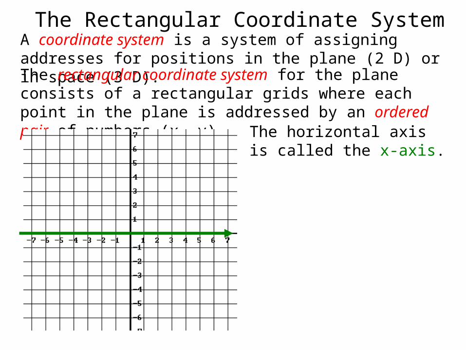
A coordinate system is a system of assigning addresses for positions in the plane (2 D) or in space (3 D). The rectangular coordinate system for the plane consists of a rectangular grids where each point in the plane is addressed by an ordered pair of numbers (x, y).
The horizontal axis is called the x-axis.
The Rectangular Coordinate System
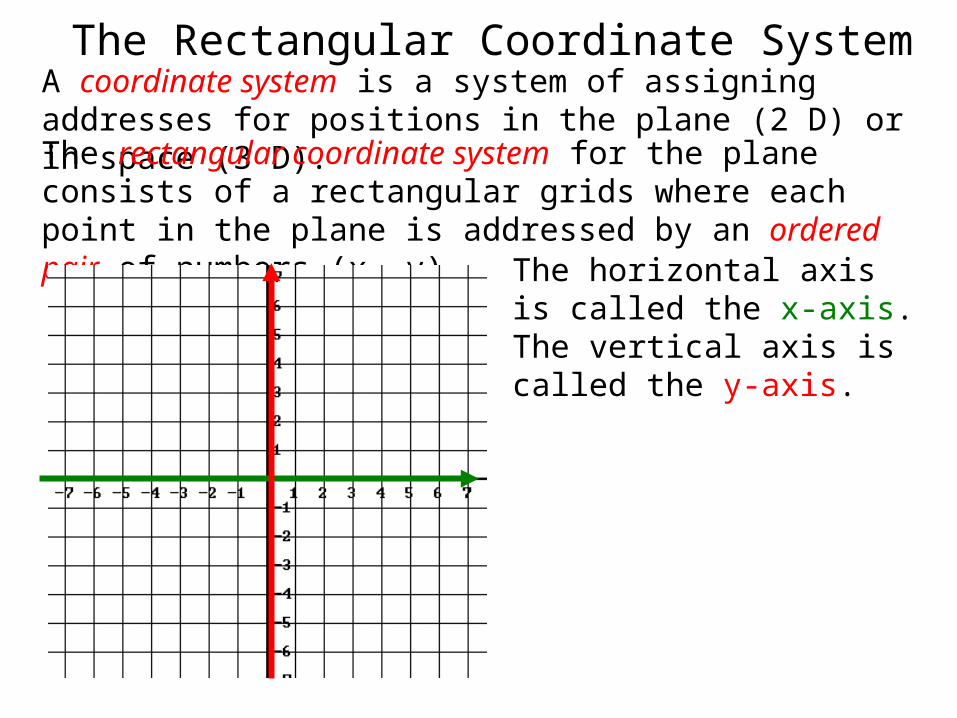
A coordinate system is a system of assigning addresses for positions in the plane (2 D) or in space (3 D). The rectangular coordinate system for the plane consists of a rectangular grids where each point in the plane is addressed by an ordered pair of numbers (x, y).
The horizontal axis is called the x-axis. The vertical axis is called the y-axis.
The Rectangular Coordinate System

A coordinate system is a system of assigning addresses for positions in the plane (2 D) or in space (3 D). The rectangular coordinate system for the plane consists of a rectangular grids where each point in the plane is addressed by an ordered pair of numbers (x, y).
The horizontal axis is called the x-axis. The vertical axis is called the y-axis. The point where the axes meet is called the origin.
The Rectangular Coordinate System
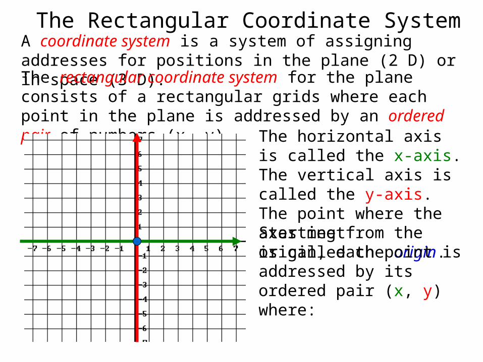
A coordinate system is a system of assigning addresses for positions in the plane (2 D) or in space (3 D). The rectangular coordinate system for the plane consists of a rectangular grids where each point in the plane is addressed by an ordered pair of numbers (x, y).
The horizontal axis is called the x-axis. The vertical axis is called the y-axis. The point where the axes meet is called the origin.Starting from the origin, each point is addressed by its ordered pair (x, y) where:
The Rectangular Coordinate System

A coordinate system is a system of assigning addresses for positions in the plane (2 D) or in space (3 D). The rectangular coordinate system for the plane consists of a rectangular grids where each point in the plane is addressed by an ordered pair of numbers (x, y).
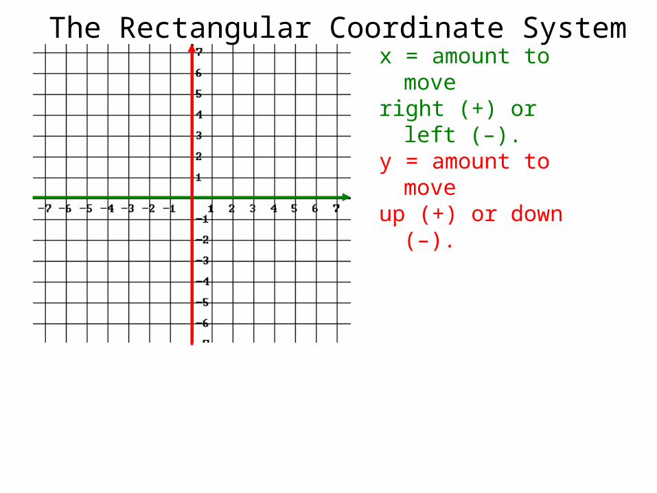
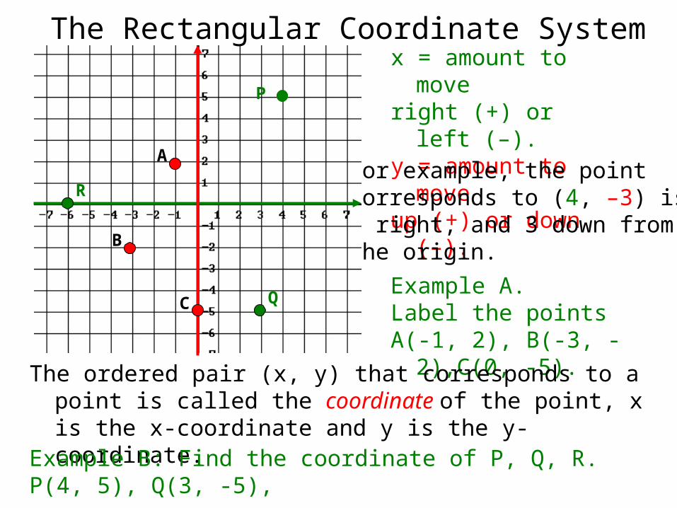
The horizontal axis is called the x-axis. The vertical axis is called the y-axis. The point where the axes meet is called the origin.Starting from the origin, each point is addressed by its ordered pair (x, y) where:x = amount to move right (+) or left (–).
The Rectangular Coordinate System

A coordinate system is a system of assigning addresses for positions in the plane (2 D) or in space (3 D). The rectangular coordinate system for the plane consists of a rectangular grids where each point in the plane is addressed by an ordered pair of numbers (x, y).
The horizontal axis is called the x-axis. The vertical axis is called the y-axis. The point where the axes meet is called the origin.Starting from the origin, each point is addressed by its ordered pair (x, y) where:x = amount to move right (+) or left (–). y = amount to moveup (+) or down (–).
The Rectangular Coordinate System
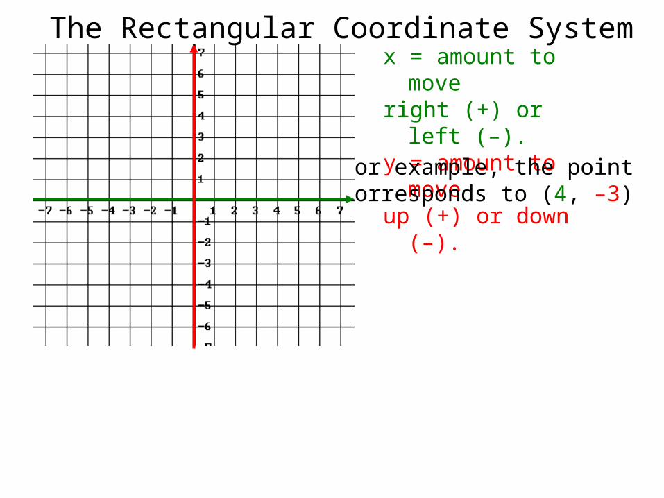
x = amount to move right (+) or left (–). y = amount to moveup (+) or down (–).
The Rectangular Coordinate System
x = amount to move right (+) or left (–). y = amount to moveup (+) or down (–).
For example, the point corresponds to (4, –3)
The Rectangular Coordinate System
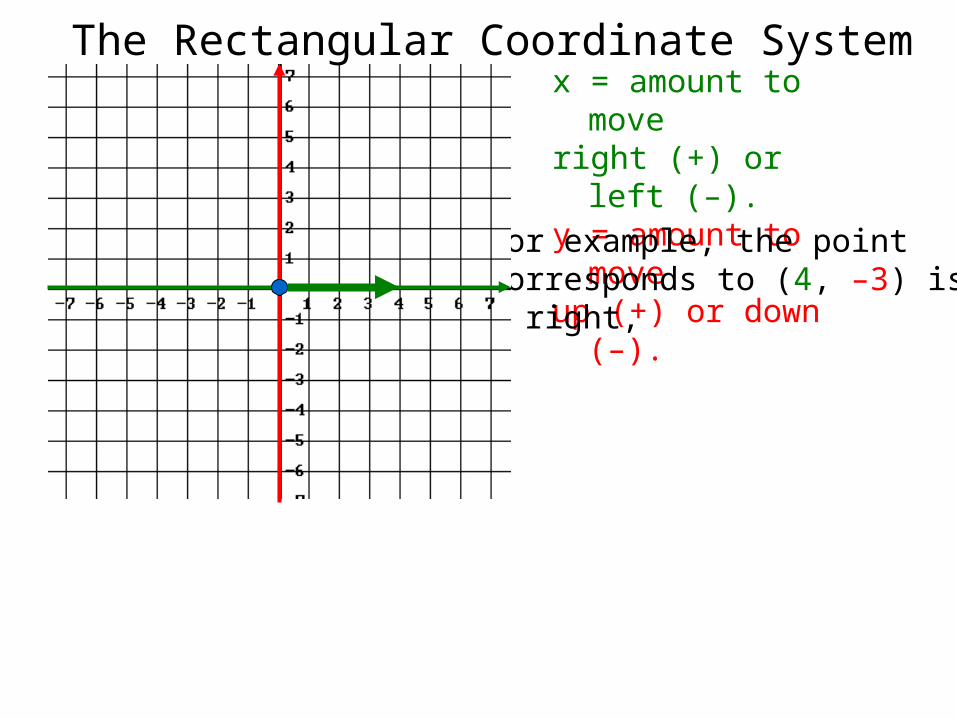
x = amount to move right (+) or left (–). y = amount to moveup (+) or down (–).
For example, the point corresponds to (4, –3) is4 right,
The Rectangular Coordinate System

x = amount to move right (+) or left (–). y = amount to moveup (+) or down (–).
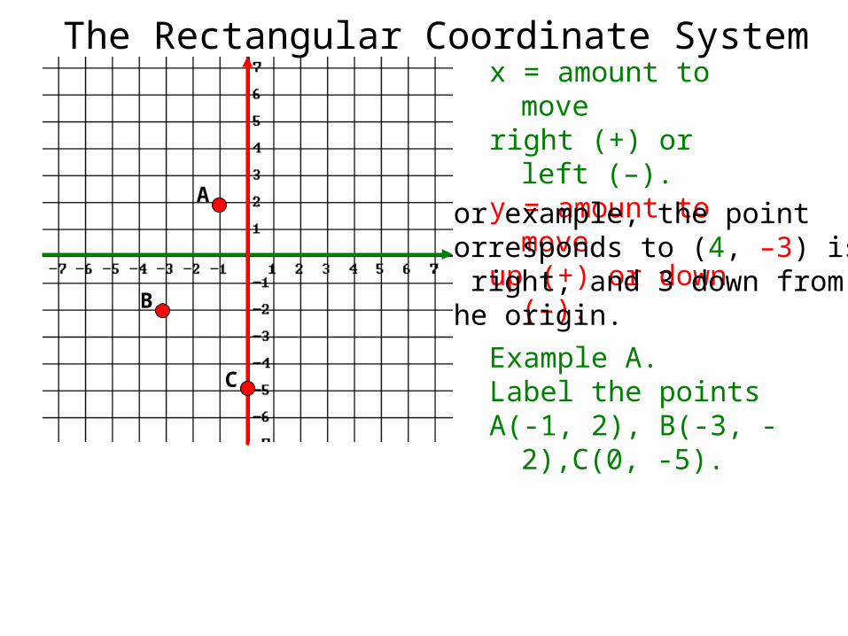
For example, the point corresponds to (4, –3) is4 right, and 3 down from the origin.
(4, –3)P
The Rectangular Coordinate System

x = amount to move right (+) or left (–). y = amount to moveup (+) or down (–).
For example, the point corresponds to (4, –3) is4 right, and 3 down from the origin.
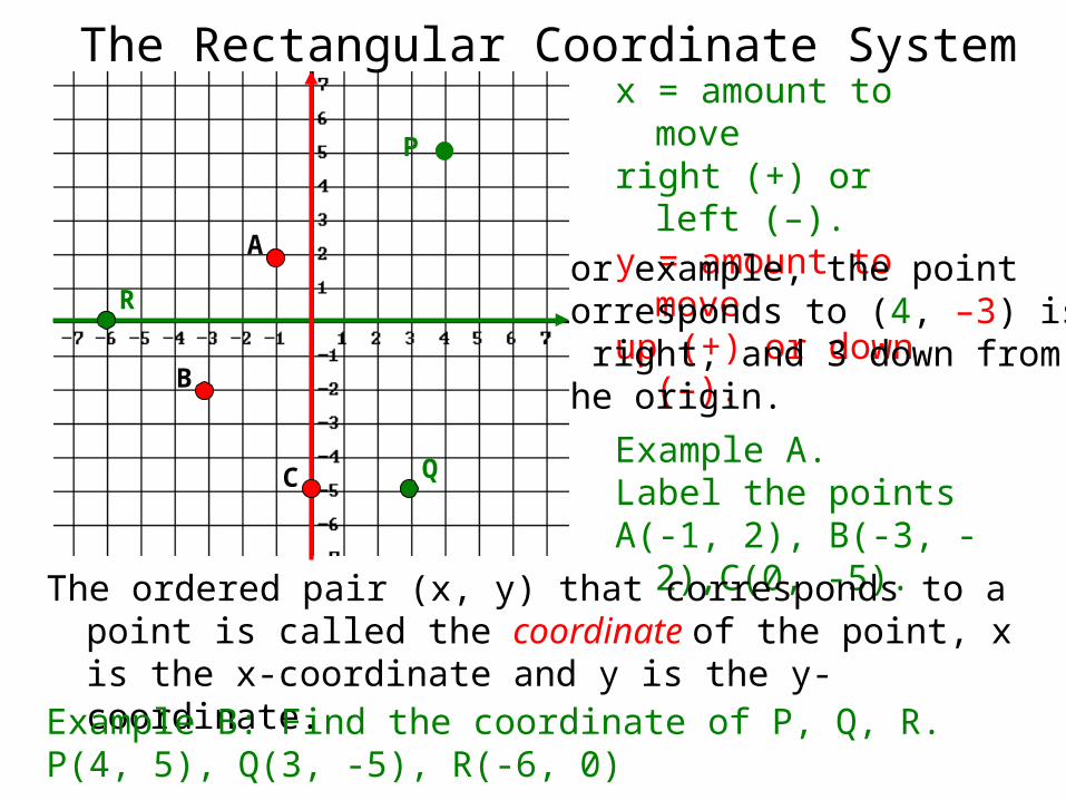
Example A. Label the points A(-1, 2), B(-3, -2),C(0, -5).
The Rectangular Coordinate System

x = amount to move right (+) or left (–). y = amount to moveup (+) or down (–).
For example, the point corresponds to (4, –3) is4 right, and 3 down from the origin.
Example A. Label the points A(-1, 2), B(-3, -2),C(0, -5).
A
The Rectangular Coordinate System

x = amount to move right (+) or left (–). y = amount to moveup (+) or down (–).
For example, the point corresponds to (4, –3) is4 right, and 3 down from the origin.
Example A. Label the points A(-1, 2), B(-3, -2),C(0, -5).
A
B
The Rectangular Coordinate System
x = amount to move right (+) or left (–). y = amount to moveup (+) or down (–).
For example, the point corresponds to (4, –3) is4 right, and 3 down from the origin.
Example A. Label the points A(-1, 2), B(-3, -2),C(0, -5).
A
B
C
The Rectangular Coordinate System

x = amount to move right (+) or left (–). y = amount to moveup (+) or down (–).
For example, the point corresponds to (4, –3) is4 right, and 3 down from the origin.
Example A. Label the points A(-1, 2), B(-3, -2),C(0, -5).
The ordered pair (x, y) that corresponds to a point is called the coordinate of the point, x is the x-coordinate and y is the y-coordinate.
A
B
C
Example B: Find the coordinate of P, Q, R.
P
Q
R
The Rectangular Coordinate System

x = amount to move right (+) or left (–). y = amount to moveup (+) or down (–).
For example, the point corresponds to (4, –3) is4 right, and 3 down from the origin.
Example A. Label the points A(-1, 2), B(-3, -2),C(0, -5).
The ordered pair (x, y) that corresponds to a point is called the coordinate of the point, x is the x-coordinate and y is the y-coordinate.
A
B
C
Example B: Find the coordinate of P, Q, R.P(4, 5),
P
Q
R
The Rectangular Coordinate System
x = amount to move right (+) or left (–). y = amount to moveup (+) or down (–).
For example, the point corresponds to (4, –3) is4 right, and 3 down from the origin.
Example A. Label the points A(-1, 2), B(-3, -2),C(0, -5).
The ordered pair (x, y) that corresponds to a point is called the coordinate of the point, x is the x-coordinate and y is the y-coordinate.
A
B
C
Example B: Find the coordinate of P, Q, R.P(4, 5), Q(3, -5),
P
Q
R
The Rectangular Coordinate System
x = amount to move right (+) or left (–). y = amount to moveup (+) or down (–).
For example, the point corresponds to (4, –3) is4 right, and 3 down from the origin.
Example A. Label the points A(-1, 2), B(-3, -2),C(0, -5).
The ordered pair (x, y) that corresponds to a point is called the coordinate of the point, x is the x-coordinate and y is the y-coordinate.
A
B
C
Example B: Find the coordinate of P, Q, R.P(4, 5), Q(3, -5), R(-6, 0)
P
Q
R
The Rectangular Coordinate System
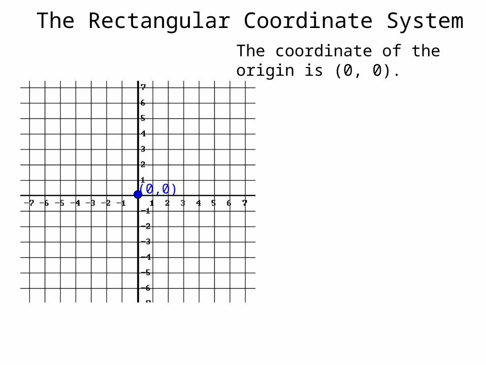
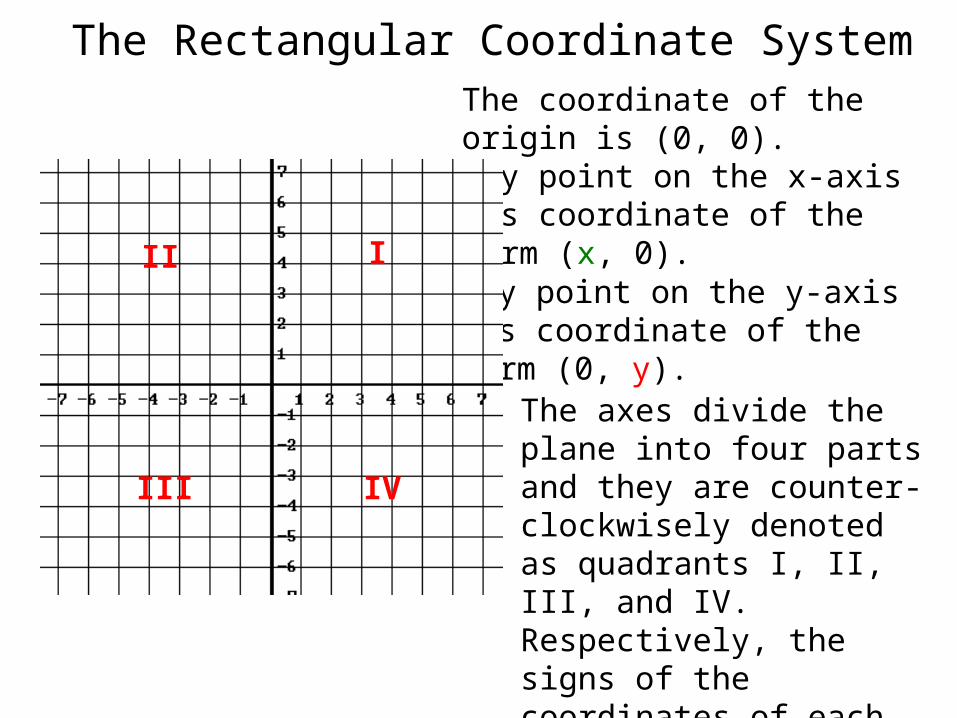
The coordinate of the origin is (0, 0).
(0,0)
The Rectangular Coordinate System

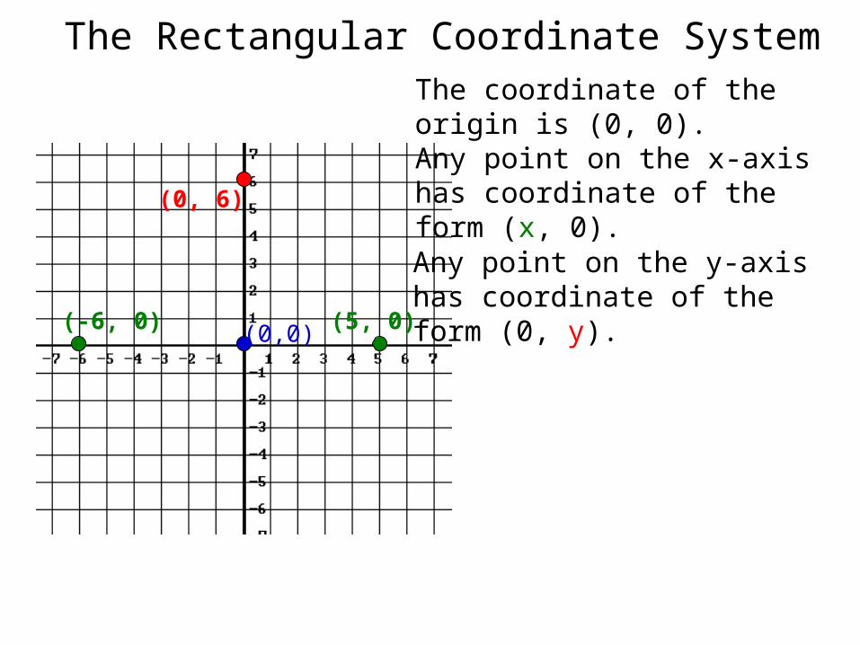
The coordinate of the origin is (0, 0).Any point on the x-axishas coordinate of the form (x, 0).
(0,0)
The Rectangular Coordinate System

The coordinate of the origin is (0, 0).Any point on the x-axishas coordinate of the form (x, 0).
(5, 0) (0,0)
The Rectangular Coordinate System

The coordinate of the origin is (0, 0).Any point on the x-axishas coordinate of the form (x, 0).
(5, 0)(-6, 0) (0,0)
The Rectangular Coordinate System

The coordinate of the origin is (0, 0).Any point on the x-axishas coordinate of the form (x, 0).
(5, 0)(-6, 0)
Any point on the y-axishas coordinate of the form (0, y). (0,0)
The Rectangular Coordinate System
The coordinate of the origin is (0, 0).Any point on the x-axishas coordinate of the form (x, 0).
(5, 0)(-6, 0)
Any point on the y-axishas coordinate of the form (0, y).
(0, 6)
(0,0)
The Rectangular Coordinate System

The coordinate of the origin is (0, 0).Any point on the x-axishas coordinate of the form (x, 0).
(5, 0)(-6, 0)
Any point on the y-axishas coordinate of the form (0, y).
(0, -4)
(0, 6)
(0,0)
The Rectangular Coordinate System

The coordinate of the origin is (0, 0).Any point on the x-axishas coordinate of the form (x, 0).Any point on the y-axishas coordinate of the form (0, y).
I II
III IV
The axes divide the plane into four parts and they are counter-clockwisely denoted as quadrants I, II, III, and IV.
The Rectangular Coordinate System
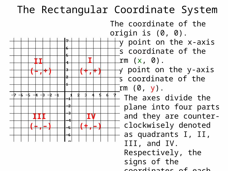
The coordinate of the origin is (0, 0).Any point on the x-axishas coordinate of the form (x, 0).Any point on the y-axishas coordinate of the form (0, y).The axes divide the plane into four parts and they are counter-clockwisely denoted as quadrants I, II, III, and IV. Respectively, the signs of the coordinates of each quadrant are shown.
I II
III IV
The Rectangular Coordinate System
The coordinate of the origin is (0, 0).Any point on the x-axishas coordinate of the form (x, 0).Any point on the y-axishas coordinate of the form (0, y).The axes divide the plane into four parts and they are counter-clockwisely denoted as quadrants I, II, III, and IV. Respectively, the signs of the coordinates of each quadrant are shown.
I II
III IV
(+,+)(–,+)
(–,–) (+,–)
The Rectangular Coordinate System
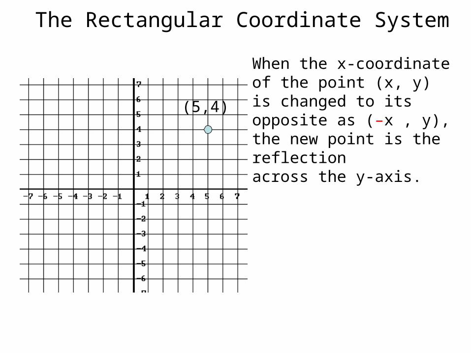
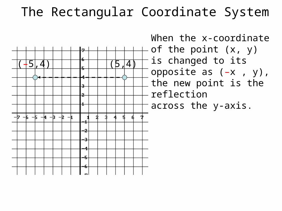
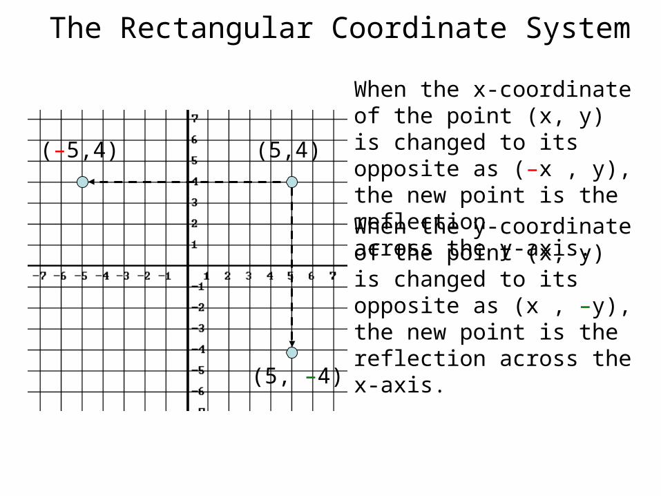
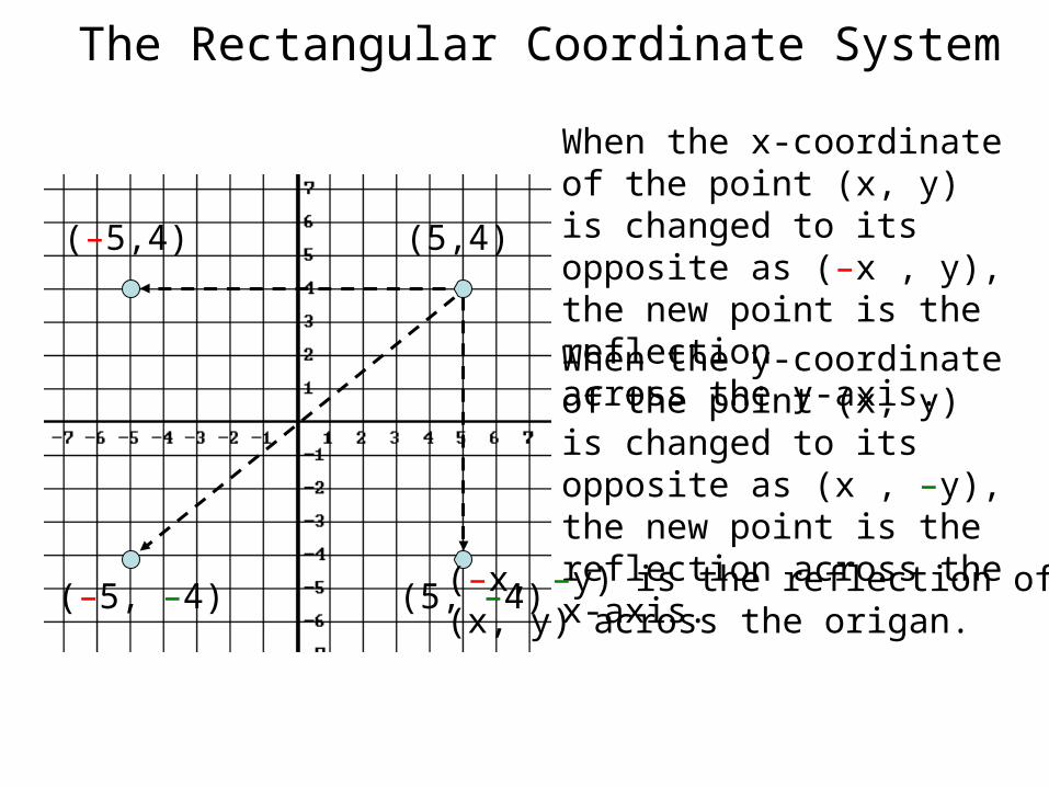
When the x-coordinate of the point (x, y) is changed to its opposite as (–x , y), the new point is the reflectionacross the y-axis.
(5,4)
The Rectangular Coordinate System
When the x-coordinate of the point (x, y) is changed to its opposite as (–x , y), the new point is the reflectionacross the y-axis.
(5,4)(–5,4)
The Rectangular Coordinate System

When the x-coordinate of the point (x, y) is changed to its opposite as (–x , y), the new point is the reflectionacross the y-axis.
When the y-coordinate of the point (x, y) is changed to its opposite as (x , –y), the new point is the reflection across the x-axis.
(5,4)(–5,4)
The Rectangular Coordinate System
When the x-coordinate of the point (x, y) is changed to its opposite as (–x , y), the new point is the reflectionacross the y-axis.
When the y-coordinate of the point (x, y) is changed to its opposite as (x , –y), the new point is the reflection across the x-axis.
(5,4)(–5,4)
(5, –4)
The Rectangular Coordinate System

When the x-coordinate of the point (x, y) is changed to its opposite as (–x , y), the new point is the reflectionacross the y-axis.
When the y-coordinate of the point (x, y) is changed to its opposite as (x , –y), the new point is the reflection across the x-axis.
(5,4)(–5,4)
(5, –4) (–x, –y) is the reflection of (x, y) across the origan.
The Rectangular Coordinate System
When the x-coordinate of the point (x, y) is changed to its opposite as (–x , y), the new point is the reflectionacross the y-axis.
When the y-coordinate of the point (x, y) is changed to its opposite as (x , –y), the new point is the reflection across the x-axis.
(5,4)(–5,4)
(5, –4) (–x, –y) is the reflection of (x, y) across the origan.
(–5, –4)
The Rectangular Coordinate System
Graphs of Lines

Graphs of LinesIn the rectangular coordinate system, ordered pairs (x, y)’s correspond to locations of points.
Graphs of LinesIn the rectangular coordinate system, ordered pairs (x, y)’s correspond to locations of points. Collections of points may be specified by the mathematical relations between the x-coordinate and the y coordinate.
Graphs of LinesIn the rectangular coordinate system, ordered pairs (x, y)’s correspond to locations of points. Collections of points may be specified by the mathematical relations between the x-coordinate and the y coordinate. The plot of points that fit a given relation is called the graph of that relation.
Graphs of LinesIn the rectangular coordinate system, ordered pairs (x, y)’s correspond to locations of points. Collections of points may be specified by the mathematical relations between the x-coordinate and the y coordinate. The plot of points that fit a given relation is called the graph of that relation. To make a graph of a given mathematical relation, make a table of points that fit the description and plot them.
Graphs of Lines
Example C. Graph the points (x, y) where x = –4
In the rectangular coordinate system, ordered pairs (x, y)’s correspond to locations of points. Collections of points may be specified by the mathematical relations between the x-coordinate and the y coordinate. The plot of points that fit a given relation is called the graph of that relation. To make a graph of a given mathematical relation, make a table of points that fit the description and plot them.

Graphs of Lines
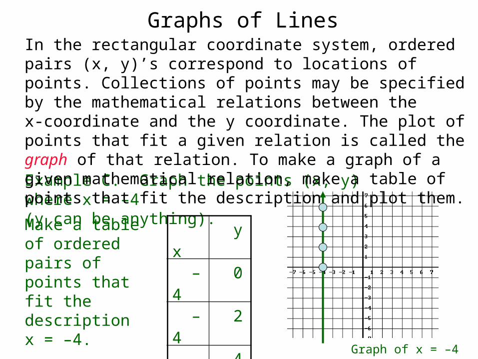
Example C. Graph the points (x, y) where x = –4 (y can be anything).
In the rectangular coordinate system, ordered pairs (x, y)’s correspond to locations of points. Collections of points may be specified by the mathematical relations between the x-coordinate and the y coordinate. The plot of points that fit a given relation is called the graph of that relation. To make a graph of a given mathematical relation, make a table of points that fit the description and plot them.

Graphs of Lines
Example C. Graph the points (x, y) where x = –4 (y can be anything).
Make a table of ordered pairs of points that fit the description x = –4.
In the rectangular coordinate system, ordered pairs (x, y)’s correspond to locations of points. Collections of points may be specified by the mathematical relations between the x-coordinate and the y coordinate. The plot of points that fit a given relation is called the graph of that relation. To make a graph of a given mathematical relation, make a table of points that fit the description and plot them.

Graphs of Lines
Example C. Graph the points (x, y) where x = –4 (y can be anything).
x y
–4
–4
–4
–4
Make a table of ordered pairs of points that fit the description x = –4.
In the rectangular coordinate system, ordered pairs (x, y)’s correspond to locations of points. Collections of points may be specified by the mathematical relations between the x-coordinate and the y coordinate. The plot of points that fit a given relation is called the graph of that relation. To make a graph of a given mathematical relation, make a table of points that fit the description and plot them.

Graphs of Lines
Example C. Graph the points (x, y) where x = –4 (y can be anything).
x y
–4 0
–4
–4
–4
Make a table of ordered pairs of points that fit the description x = –4.
In the rectangular coordinate system, ordered pairs (x, y)’s correspond to locations of points. Collections of points may be specified by the mathematical relations between the x-coordinate and the y coordinate. The plot of points that fit a given relation is called the graph of that relation. To make a graph of a given mathematical relation, make a table of points that fit the description and plot them.

Graphs of Lines
Example C. Graph the points (x, y) where x = –4 (y can be anything).
x y
–4 0
–4 2
–4
–4
Make a table of ordered pairs of points that fit the description x = –4.
In the rectangular coordinate system, ordered pairs (x, y)’s correspond to locations of points. Collections of points may be specified by the mathematical relations between the x-coordinate and the y coordinate. The plot of points that fit a given relation is called the graph of that relation. To make a graph of a given mathematical relation, make a table of points that fit the description and plot them.

Graphs of Lines
Example C. Graph the points (x, y) where x = –4 (y can be anything).
x y
–4 0
–4 2
–4 4
–4 6
Make a table of ordered pairs of points that fit the description x = –4.
In the rectangular coordinate system, ordered pairs (x, y)’s correspond to locations of points. Collections of points may be specified by the mathematical relations between the x-coordinate and the y coordinate. The plot of points that fit a given relation is called the graph of that relation. To make a graph of a given mathematical relation, make a table of points that fit the description and plot them.
Graphs of Lines
Example C. Graph the points (x, y) where x = –4 (y can be anything).
x y
–4 0
–4 2
–4 4
–4 6
Graph of x = –4
Make a table of ordered pairs of points that fit the description x = –4.
In the rectangular coordinate system, ordered pairs (x, y)’s correspond to locations of points. Collections of points may be specified by the mathematical relations between the x-coordinate and the y coordinate. The plot of points that fit a given relation is called the graph of that relation. To make a graph of a given mathematical relation, make a table of points that fit the description and plot them.

Graphs of LinesFirst degree equation in the variables x and y are equations that may be put into the form Ax + By = C where A, B, C are numbers.

Graphs of LinesFirst degree equation in the variables x and y are equations that may be put into the form Ax + By = C where A, B, C are numbers. First degree equations are the same as linear equations.

Graphs of LinesFirst degree equation in the variables x and y are equations that may be put into the form Ax + By = C where A, B, C are numbers. First degree equations are the same as linear equations. They are called linear because their graphs are straight lines.
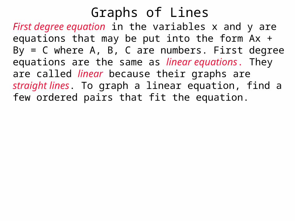
Graphs of LinesFirst degree equation in the variables x and y are equations that may be put into the form Ax + By = C where A, B, C are numbers. First degree equations are the same as linear equations. They are called linear because their graphs are straight lines. To graph a linear equation, find a few ordered pairs that fit the equation.
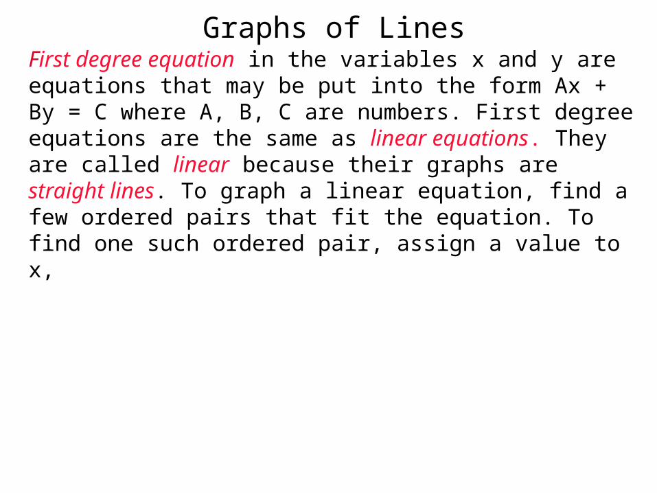
Graphs of LinesFirst degree equation in the variables x and y are equations that may be put into the form Ax + By = C where A, B, C are numbers. First degree equations are the same as linear equations. They are called linear because their graphs are straight lines. To graph a linear equation, find a few ordered pairs that fit the equation. To find one such ordered pair, assign a value to x,
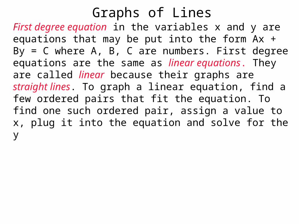
Graphs of LinesFirst degree equation in the variables x and y are equations that may be put into the form Ax + By = C where A, B, C are numbers. First degree equations are the same as linear equations. They are called linear because their graphs are straight lines. To graph a linear equation, find a few ordered pairs that fit the equation. To find one such ordered pair, assign a value to x, plug it into the equation and solve for the y

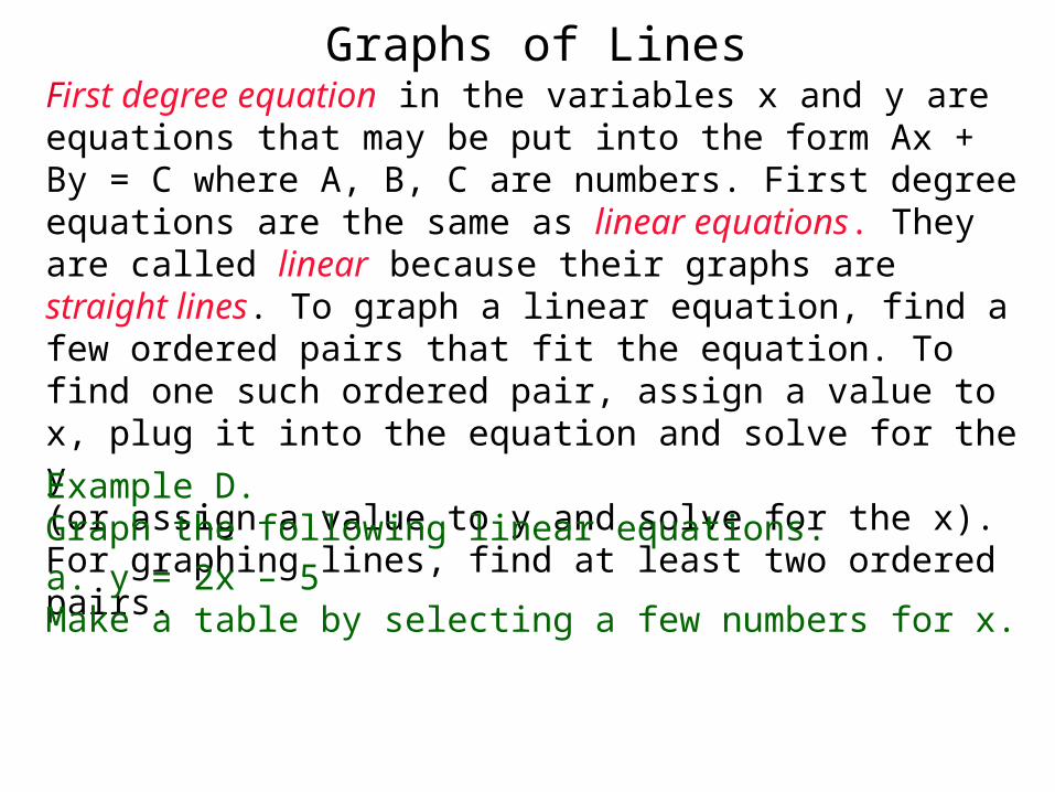
Graphs of LinesFirst degree equation in the variables x and y are equations that may be put into the form Ax + By = C where A, B, C are numbers. First degree equations are the same as linear equations. They are called linear because their graphs are straight lines. To graph a linear equation, find a few ordered pairs that fit the equation. To find one such ordered pair, assign a value to x, plug it into the equation and solve for the y (or assign a value to y and solve for the x).

Graphs of LinesFirst degree equation in the variables x and y are equations that may be put into the form Ax + By = C where A, B, C are numbers. First degree equations are the same as linear equations. They are called linear because their graphs are straight lines. To graph a linear equation, find a few ordered pairs that fit the equation. To find one such ordered pair, assign a value to x, plug it into the equation and solve for the y (or assign a value to y and solve for the x). For graphing lines, find at least two ordered pairs.

Graphs of LinesFirst degree equation in the variables x and y are equations that may be put into the form Ax + By = C where A, B, C are numbers. First degree equations are the same as linear equations. They are called linear because their graphs are straight lines. To graph a linear equation, find a few ordered pairs that fit the equation. To find one such ordered pair, assign a value to x, plug it into the equation and solve for the y (or assign a value to y and solve for the x). For graphing lines, find at least two ordered pairs.
Example D. Graph the following linear equations.
a. y = 2x – 5
Graphs of LinesFirst degree equation in the variables x and y are equations that may be put into the form Ax + By = C where A, B, C are numbers. First degree equations are the same as linear equations. They are called linear because their graphs are straight lines. To graph a linear equation, find a few ordered pairs that fit the equation. To find one such ordered pair, assign a value to x, plug it into the equation and solve for the y (or assign a value to y and solve for the x). For graphing lines, find at least two ordered pairs.
Example D. Graph the following linear equations.
a. y = 2x – 5Make a table by selecting a few numbers for x.

Graphs of LinesFirst degree equation in the variables x and y are equations that may be put into the form Ax + By = C where A, B, C are numbers. First degree equations are the same as linear equations. They are called linear because their graphs are straight lines. To graph a linear equation, find a few ordered pairs that fit the equation. To find one such ordered pair, assign a value to x, plug it into the equation and solve for the y (or assign a value to y and solve for the x). For graphing lines, find at least two ordered pairs.
Example D. Graph the following linear equations.
a. y = 2x – 5Make a table by selecting a few numbers for x. For easy calculations we set x = -1, 0, 1, and 2.

Graphs of LinesFirst degree equation in the variables x and y are equations that may be put into the form Ax + By = C where A, B, C are numbers. First degree equations are the same as linear equations. They are called linear because their graphs are straight lines. To graph a linear equation, find a few ordered pairs that fit the equation. To find one such ordered pair, assign a value to x, plug it into the equation and solve for the y (or assign a value to y and solve for the x). For graphing lines, find at least two ordered pairs.
Example D. Graph the following linear equations.
a. y = 2x – 5Make a table by selecting a few numbers for x. For easy calculations we set x = -1, 0, 1, and 2. Plug each of these values into x and find its corresponding y to form an ordered pair.

Graphs of LinesFor y = 2x – 5:
x y
-1
0
1
2
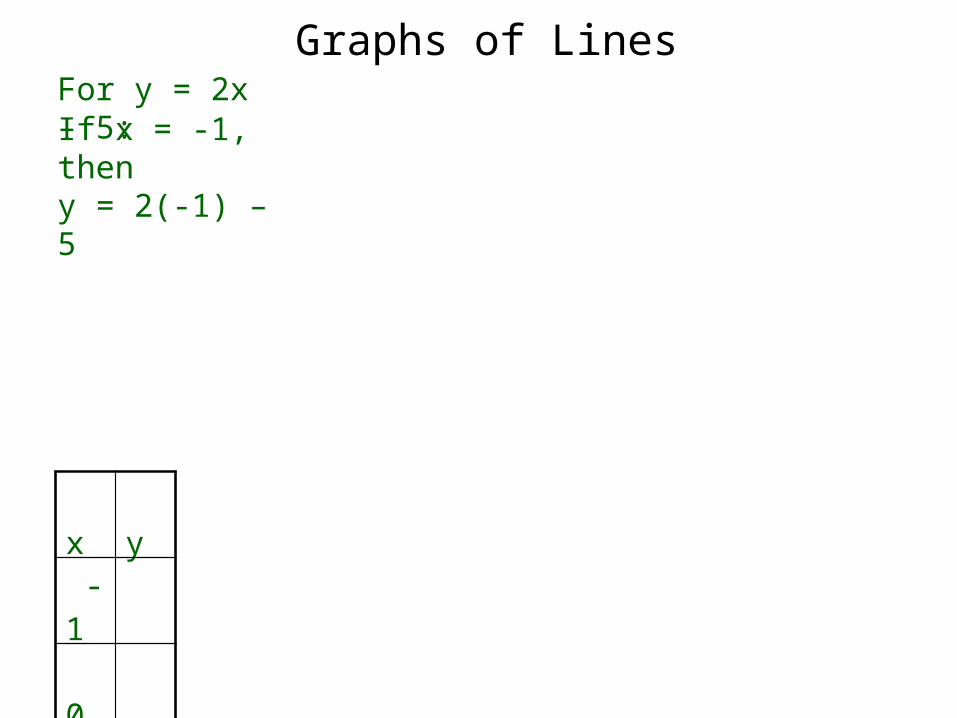
Graphs of LinesFor y = 2x – 5:
x y
-1
0
1
2
If x = -1, then y = 2(-1) – 5
Graphs of LinesFor y = 2x – 5:
x y
-1 -7
0
1
2
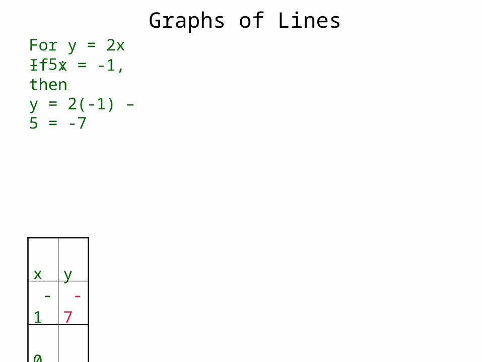
If x = -1, then y = 2(-1) – 5 = -7

Graphs of LinesFor y = 2x – 5:
x y
-1 -7
0 -5
1
2
If x = -1, then y = 2(-1) – 5 = -7
If x = 0, then y = 2(0) – 5

Graphs of LinesFor y = 2x – 5:
x y
-1 -7
0 -5
1
2
If x = -1, then y = 2(-1) – 5 = -7
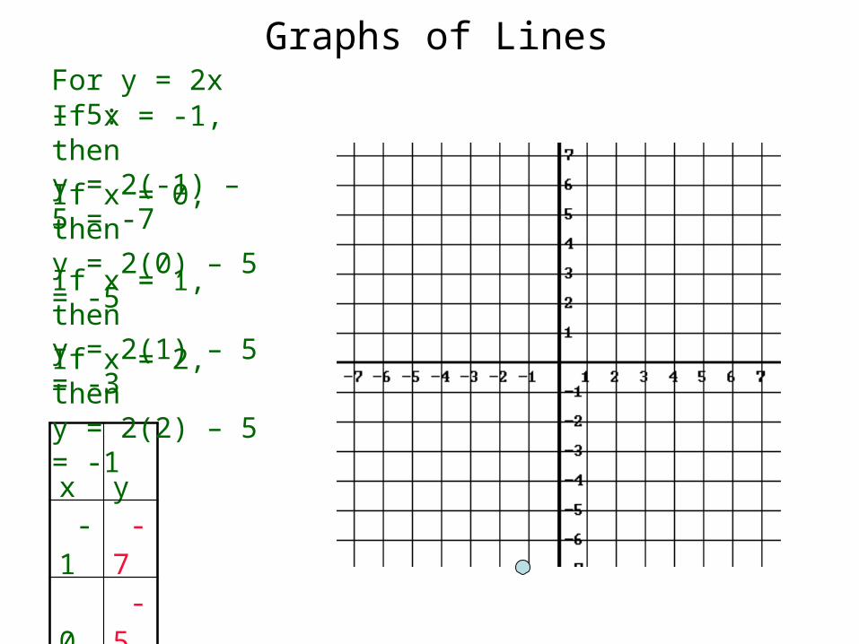
If x = 0, then y = 2(0) – 5 = -5

Graphs of LinesFor y = 2x – 5:
x y
-1 -7
0 -5
1 -3
2 -1
If x = -1, then y = 2(-1) – 5 = -7
If x = 0, then y = 2(0) – 5 = -5
If x = 1, then y = 2(1) – 5 = -3
If x = 2, then y = 2(2) – 5 = -1

Graphs of LinesFor y = 2x – 5:
x y
-1 -7
0 -5
1 -3
2 -1
If x = -1, then y = 2(-1) – 5 = -7
If x = 0, then y = 2(0) – 5 = -5
If x = 1, then y = 2(1) – 5 = -3
If x = 2, then y = 2(2) – 5 = -1
Graphs of LinesFor y = 2x – 5:
x y
-1 -7
0 -5
1 -3
2 -1
If x = -1, then y = 2(-1) – 5 = -7
If x = 0, then y = 2(0) – 5 = -5
If x = 1, then y = 2(1) – 5 = -3
If x = 2, then y = 2(2) – 5 = -1

Graphs of LinesFor y = 2x – 5:
x y
-1 -7
0 -5
1 -3
2 -1
If x = -1, then y = 2(-1) – 5 = -7
If x = 0, then y = 2(0) – 5 = -5
If x = 1, then y = 2(1) – 5 = -3
If x = 2, then y = 2(2) – 5 = -1

Graphs of LinesFor y = 2x – 5:
x y
-1 -7
0 -5
1 -3
2 -1
If x = -1, then y = 2(-1) – 5 = -7
If x = 0, then y = 2(0) – 5 = -5
If x = 1, then y = 2(1) – 5 = -3
If x = 2, then y = 2(2) – 5 = -1

Graphs of LinesFor y = 2x – 5:
x y
-1 -7
0 -5
1 -3
2 -1
If x = -1, then y = 2(-1) – 5 = -7
If x = 0, then y = 2(0) – 5 = -5
If x = 1, then y = 2(1) – 5 = -3
If x = 2, then y = 2(2) – 5 = -1
b. -3y = 12 Graphs of Lines

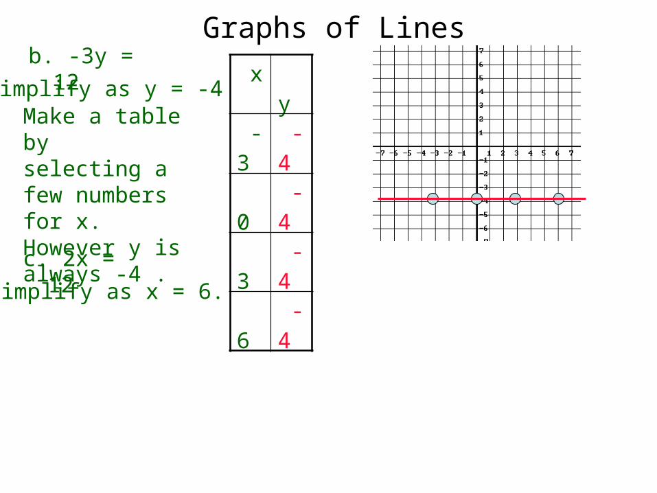
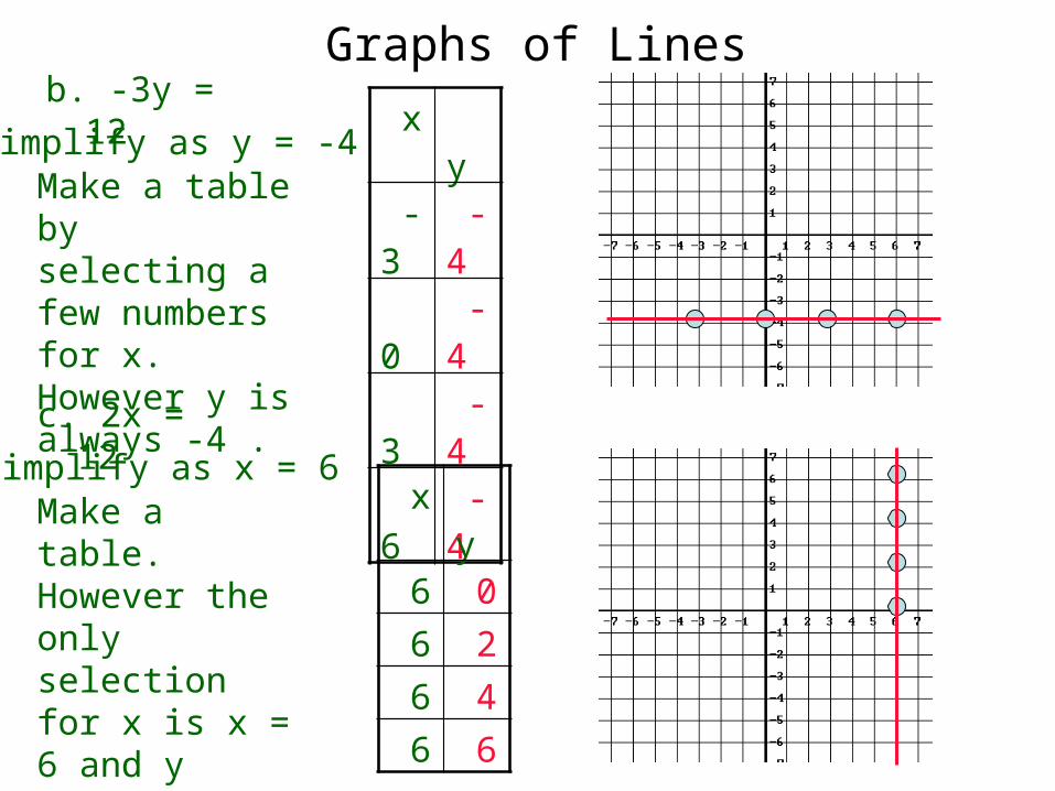
b. -3y = 12
Simplify as y = -4
Graphs of Lines
Make a table by selecting a few numbers for x.

b. -3y = 12
Simplify as y = -4
Graphs of Lines
Make a table by selecting a few numbers for x.
x y
-3
0
3
6

b. -3y = 12
Simplify as y = -4
Graphs of Lines
Make a table by selecting a few numbers for x. However y is always -4 .
x y
-3 -4
0 -4
3 -4
6 -4

b. -3y = 12
Simplify as y = -4
Graphs of Lines
Make a table by selecting a few numbers for x. However y is always -4 .
x y
-3 -4
0 -4
3 -4
6 -4

b. -3y = 12
Simplify as y = -4
Graphs of Lines
Make a table by selecting a few numbers for x. However y is always -4 .
x y
-3 -4
0 -4
3 -4
6 -4

b. -3y = 12
Simplify as y = -4
Graphs of Lines
Make a table by selecting a few numbers for x. However y is always -4 .
x y
-3 -4
0 -4
3 -4
6 -4

b. -3y = 12
Simplify as y = -4
Graphs of Lines
c. 2x = 12
Make a table by selecting a few numbers for x. However y is always -4 .
x y
-3 -4
0 -4
3 -4
6 -4
b. -3y = 12
Simplify as y = -4
Graphs of Lines
c. 2x = 12
Make a table by selecting a few numbers for x. However y is always -4 .
x y
-3 -4
0 -4
3 -4
6 -4
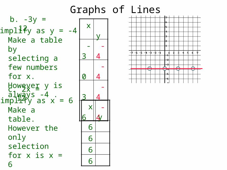
Simplify as x = 6.

b. -3y = 12
Simplify as y = -4
Graphs of Lines
c. 2x = 12
Make a table by selecting a few numbers for x. However y is always -4 .
x y
-3 -4
0 -4
3 -4
6 -4
Simplify as x = 6 Make a table. However the only selection for x is x = 6
b. -3y = 12
Simplify as y = -4
Graphs of Lines
c. 2x = 12
Make a table by selecting a few numbers for x. However y is always -4 .
x y
-3 -4
0 -4
3 -4
6 -4
Simplify as x = 6 Make a table. However the only selection for x is x = 6
x y
6
6
6
6

b. -3y = 12
Simplify as y = -4
Graphs of Lines
c. 2x = 12
Make a table by selecting a few numbers for x. However y is always -4 .
x y
-3 -4
0 -4
3 -4
6 -4
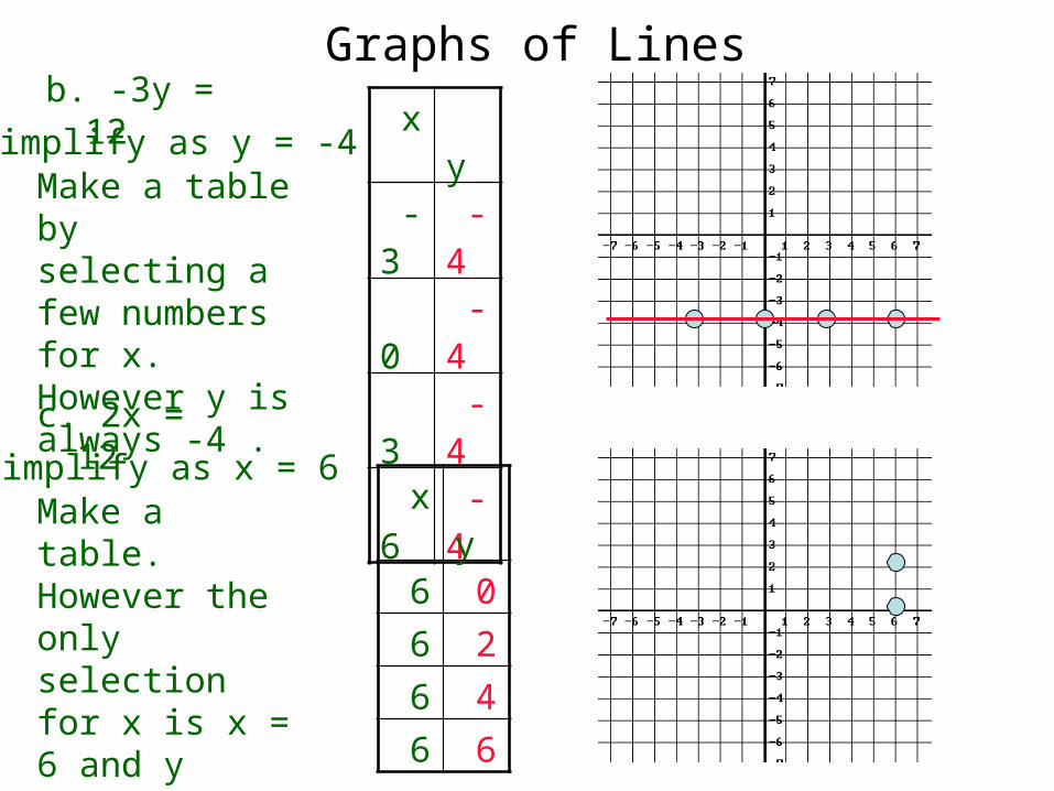
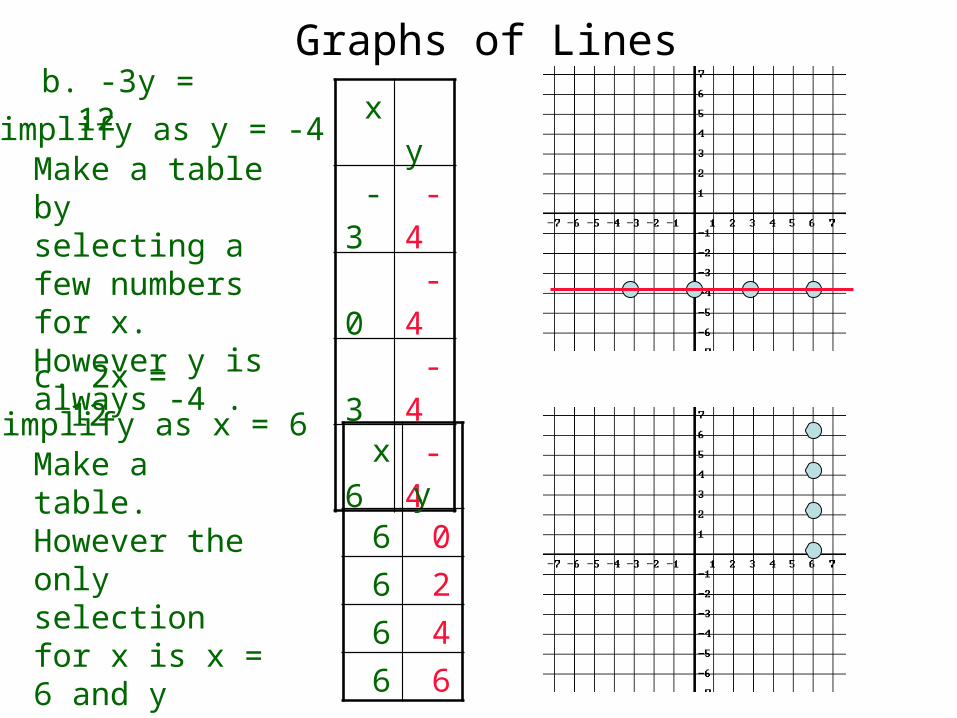
Simplify as x = 6 Make a table. However the only selection for x is x = 6 and y could be any number.
x y
6 0
6 2
6 4
6 6

b. -3y = 12
Simplify as y = -4
Graphs of Lines
c. 2x = 12
Make a table by selecting a few numbers for x. However y is always -4 .
x y
-3 -4
0 -4
3 -4
6 -4
Simplify as x = 6 Make a table. However the only selection for x is x = 6 and y could be any number.
x y
6 0
6 2
6 4
6 6
b. -3y = 12
Simplify as y = -4
Graphs of Lines
c. 2x = 12
Make a table by selecting a few numbers for x. However y is always -4 .
x y
-3 -4
0 -4
3 -4
6 -4
Simplify as x = 6 Make a table. However the only selection for x is x = 6 and y could be any number.
x y
6 0
6 2
6 4
6 6
b. -3y = 12
Simplify as y = -4
Graphs of Lines
c. 2x = 12
Make a table by selecting a few numbers for x. However y is always -4 .
x y
-3 -4
0 -4
3 -4
6 -4
Simplify as x = 6 Make a table. However the only selection for x is x = 6 and y could be any number.
x y
6 0
6 2
6 4
6 6
b. -3y = 12
Simplify as y = -4
Graphs of Lines
c. 2x = 12
Make a table by selecting a few numbers for x. However y is always -4 .
x y
-3 -4
0 -4
3 -4
6 -4
Simplify as x = 6 Make a table. However the only selection for x is x = 6 and y could be any number.
x y
6 0
6 2
6 4
6 6

Summary of the graphs of linear equations:
Graphs of Lines

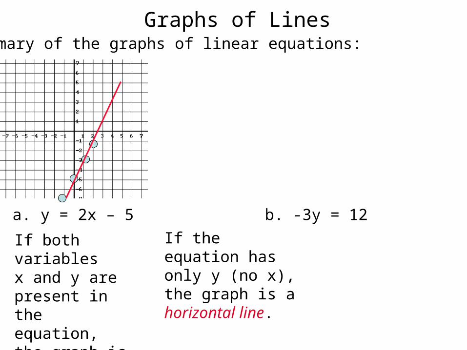
a. y = 2x – 5
Summary of the graphs of linear equations:
Graphs of Lines

a. y = 2x – 5
If both variables x and y are present in theequation, the graph is a tilted line.
Summary of the graphs of linear equations:
Graphs of Lines

a. y = 2x – 5
If both variables x and y are present in theequation, the graph is a tilted line.
Summary of the graphs of linear equations:
Graphs of Lines

a. y = 2x – 5 b. -3y = 12
If both variables x and y are present in theequation, the graph is a tilted line.
Summary of the graphs of linear equations:
Graphs of Lines
a. y = 2x – 5 b. -3y = 12
If both variables x and y are present in theequation, the graph is a tilted line.
If the equation has only y (no x), the graph is a horizontal line.
Summary of the graphs of linear equations:
Graphs of Lines
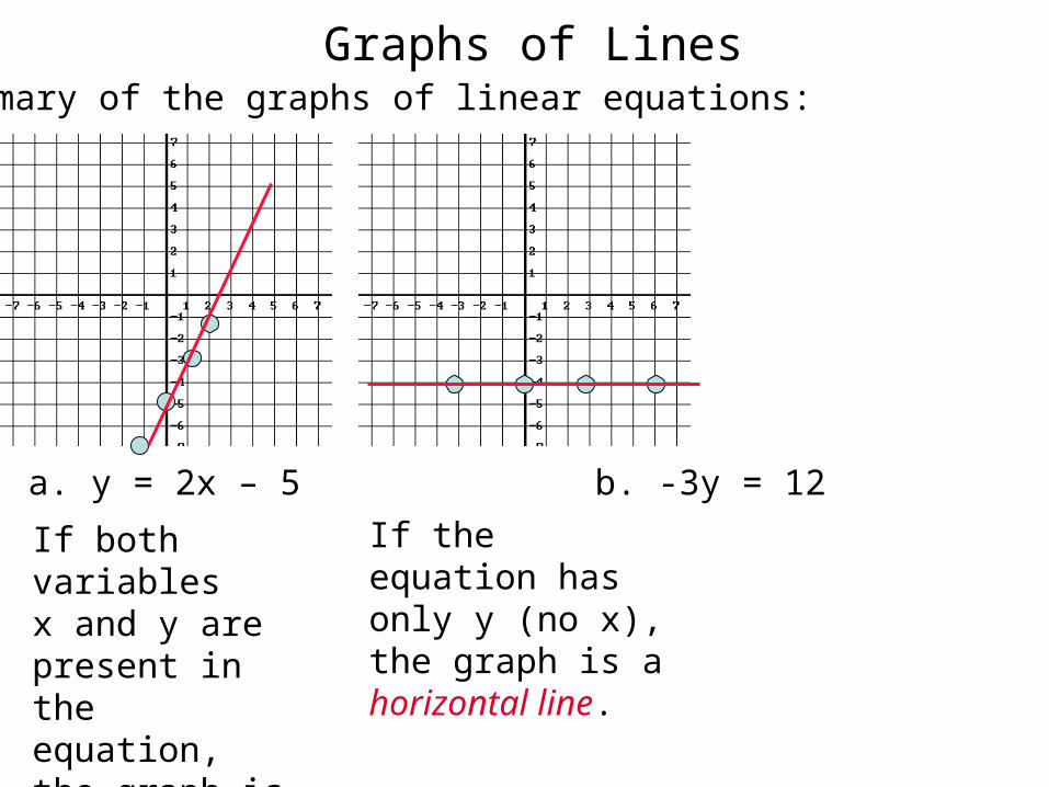
a. y = 2x – 5 b. -3y = 12
If both variables x and y are present in theequation, the graph is a tilted line.
If the equation has only y (no x), the graph is a horizontal line.
Summary of the graphs of linear equations:
Graphs of Lines

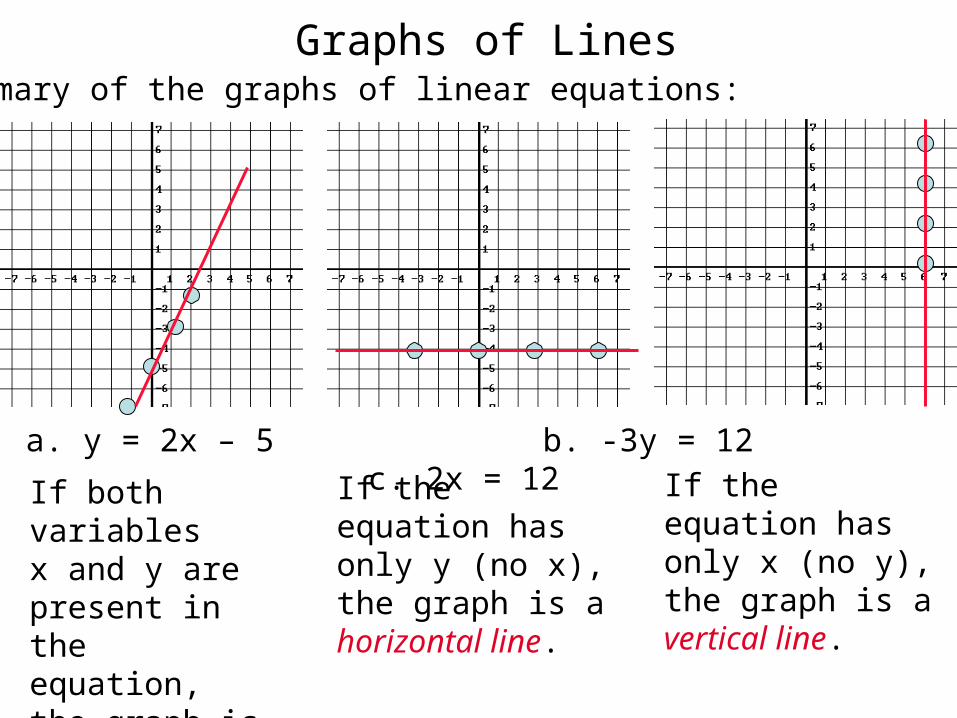
a. y = 2x – 5 b. -3y = 12 c. 2x = 12
If both variables x and y are present in theequation, the graph is a tilted line.
If the equation has only y (no x), the graph is a horizontal line.
Summary of the graphs of linear equations:
Graphs of Lines

a. y = 2x – 5 b. -3y = 12 c. 2x = 12
If both variables x and y are present in theequation, the graph is a tilted line.
If the equation has only y (no x), the graph is a horizontal line.
Summary of the graphs of linear equations:
Graphs of Lines
If the equation has only x (no y), the graph is a vertical line.

x-Intercepts is where the line crosses the x-axis; Graphs of Lines

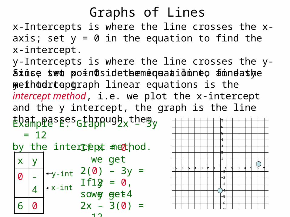
x-Intercepts is where the line crosses the x-axis; set y = 0 in the equation to find the x-intercept.
Graphs of Lines
x-Intercepts is where the line crosses the x-axis; set y = 0 in the equation to find the x-intercept. y-Intercepts is where the line crosses the y-axis;
Graphs of Lines
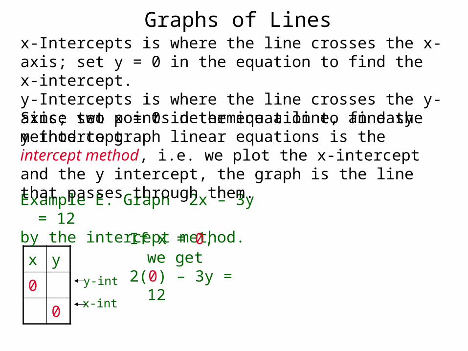
x-Intercepts is where the line crosses the x-axis; set y = 0 in the equation to find the x-intercept. y-Intercepts is where the line crosses the y-axis; set x = 0 in the equation to find the y-intercept.
Graphs of Lines

x-Intercepts is where the line crosses the x-axis; set y = 0 in the equation to find the x-intercept. y-Intercepts is where the line crosses the y-axis; set x = 0 in the equation to find the y-intercept.
Graphs of Lines
Since two points determine a line, an easy method to graph linear equations is the intercept method,
x-Intercepts is where the line crosses the x-axis; set y = 0 in the equation to find the x-intercept. y-Intercepts is where the line crosses the y-axis; set x = 0 in the equation to find the y-intercept.
Graphs of Lines
Since two points determine a line, an easy method to graph linear equations is the intercept method, i.e. we plot the x-intercept and the y intercept, the graph is the line that passes through them.

x-Intercepts is where the line crosses the x-axis; set y = 0 in the equation to find the x-intercept. y-Intercepts is where the line crosses the y-axis; set x = 0 in the equation to find the y-intercept.
Graphs of Lines
Example E. Graph 2x – 3y = 12by the intercept method.
Since two points determine a line, an easy method to graph linear equations is the intercept method, i.e. we plot the x-intercept and the y intercept, the graph is the line that passes through them.

x y
0
0
x-Intercepts is where the line crosses the x-axis; set y = 0 in the equation to find the x-intercept. y-Intercepts is where the line crosses the y-axis; set x = 0 in the equation to find the y-intercept.
y-int
x-int
Graphs of Lines
Example E. Graph 2x – 3y = 12by the intercept method.
Since two points determine a line, an easy method to graph linear equations is the intercept method, i.e. we plot the x-intercept and the y intercept, the graph is the line that passes through them.
If x = 0, we get 2(0) – 3y = 12

x y
0 -4
0
x-Intercepts is where the line crosses the x-axis; set y = 0 in the equation to find the x-intercept. y-Intercepts is where the line crosses the y-axis; set x = 0 in the equation to find the y-intercept.
y-int
x-int
Graphs of Lines
Example E. Graph 2x – 3y = 12by the intercept method.
Since two points determine a line, an easy method to graph linear equations is the intercept method, i.e. we plot the x-intercept and the y intercept, the graph is the line that passes through them.
If x = 0, we get 2(0) – 3y = 12 so y = -4

x y
0 -4
0
x-Intercepts is where the line crosses the x-axis; set y = 0 in the equation to find the x-intercept. y-Intercepts is where the line crosses the y-axis; set x = 0 in the equation to find the y-intercept.
y-int
x-int
Graphs of Lines
Example E. Graph 2x – 3y = 12by the intercept method.
Since two points determine a line, an easy method to graph linear equations is the intercept method, i.e. we plot the x-intercept and the y intercept, the graph is the line that passes through them.
If x = 0, we get 2(0) – 3y = 12 so y = -4If y = 0, we get 2x – 3(0) = 12

x y
0 -4
6 0
x-Intercepts is where the line crosses the x-axis; set y = 0 in the equation to find the x-intercept. y-Intercepts is where the line crosses the y-axis; set x = 0 in the equation to find the y-intercept.
y-int
x-int
Graphs of Lines
Example E. Graph 2x – 3y = 12by the intercept method.
Since two points determine a line, an easy method to graph linear equations is the intercept method, i.e. we plot the x-intercept and the y intercept, the graph is the line that passes through them.
If x = 0, we get 2(0) – 3y = 12 so y = -4If y = 0, we get 2x – 3(0) = 12 so x = 6
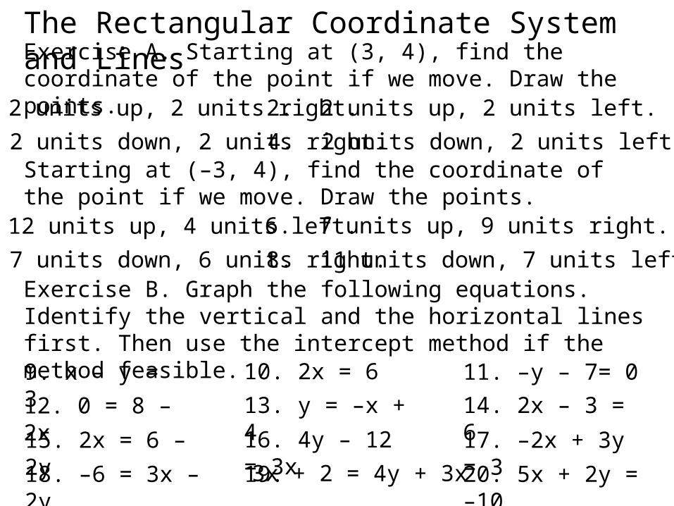
Exercise B. Graph the following equations. Identify the vertical and the horizontal lines first. Then use the intercept method if the method feasible.9. x – y = 3 10. 2x = 6 11. –y – 7= 0
12. 0 = 8 – 2x 13. y = –x + 4 14. 2x – 3 = 6
15. 2x = 6 – 2y 16. 4y – 12 = 3x 17. –2x + 3y = 3
18. –6 = 3x – 2y 19. 3x + 2 = 4y + 3x 20. 5x + 2y = –10
The Rectangular Coordinate System and LinesExercise A. Starting at (3, 4), find the coordinate of the point if we move. Draw the points.1. 2 units up, 2 units right. 2. 2 units up, 2 units left.
3. 2 units down, 2 units right. 4. 2 units down, 2 units left.Starting at (–3, 4), find the coordinate of the point if we move. Draw the points.
6. 7 units up, 9 units right.5. 12 units up, 4 units left.
7. 7 units down, 6 units right. 8. 11 units down, 7 units left.