1

Heuristic Search4 4.0 Introduction

4.1 An Algorithm forHeuristic Search

4.2 Admissibility, Monotonicity, andInformedness

4.3 Using Heuristicsin Games

4.4 Complexity Issues

4.5 Epilogue and References

4.6 Exercises

Additional references for the slides:

Russell and Norvig’s AI book (2003).

Robert Wilensky’s CS188 slides: www.cs.berkeley.edu/~wilensky/cs188/lectures/index.html

Tim Huang’s slides for the game of Go.

2

Chapter Objectives

• Learn the basics of heuristic search in a state space.

• Learn the basic properties of heuristics: admissability, monotonicity, informedness.

• Learn the basics of searching for two-person games: minimax algorithm and alpha-beta procedure.

• The agent model: Has a problem, searches for a solution, has some “heuristics” to speed up the search.

3

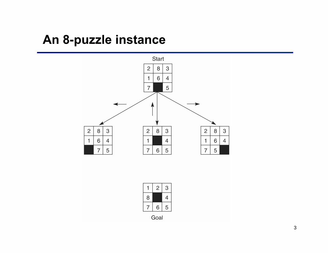
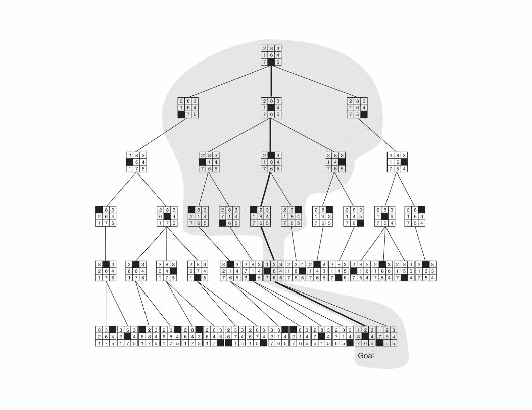
An 8-puzzle instance

4

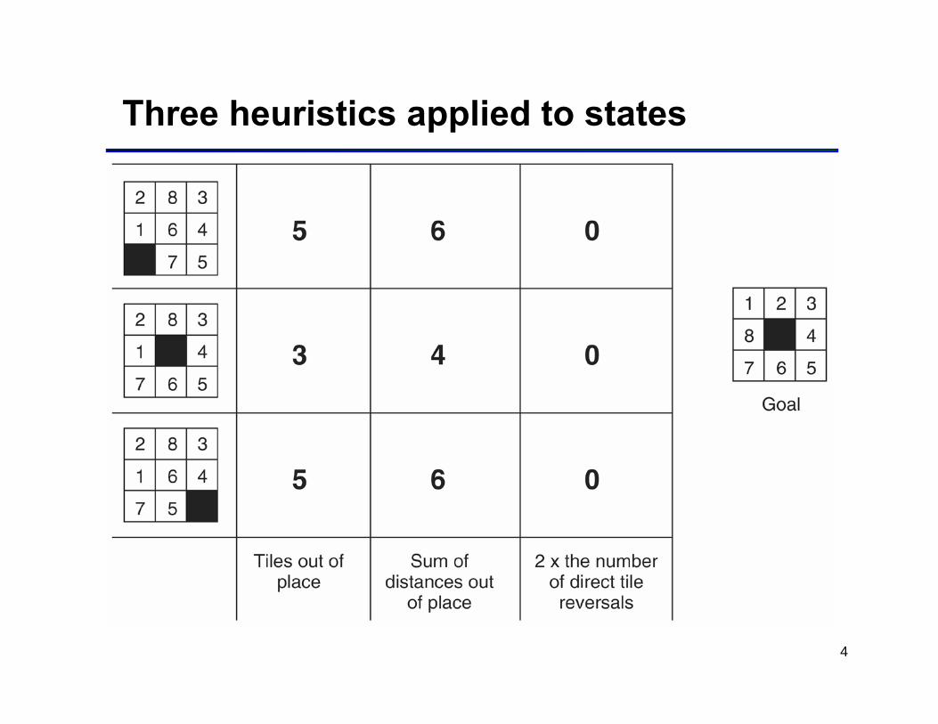
Three heuristics applied to states

5

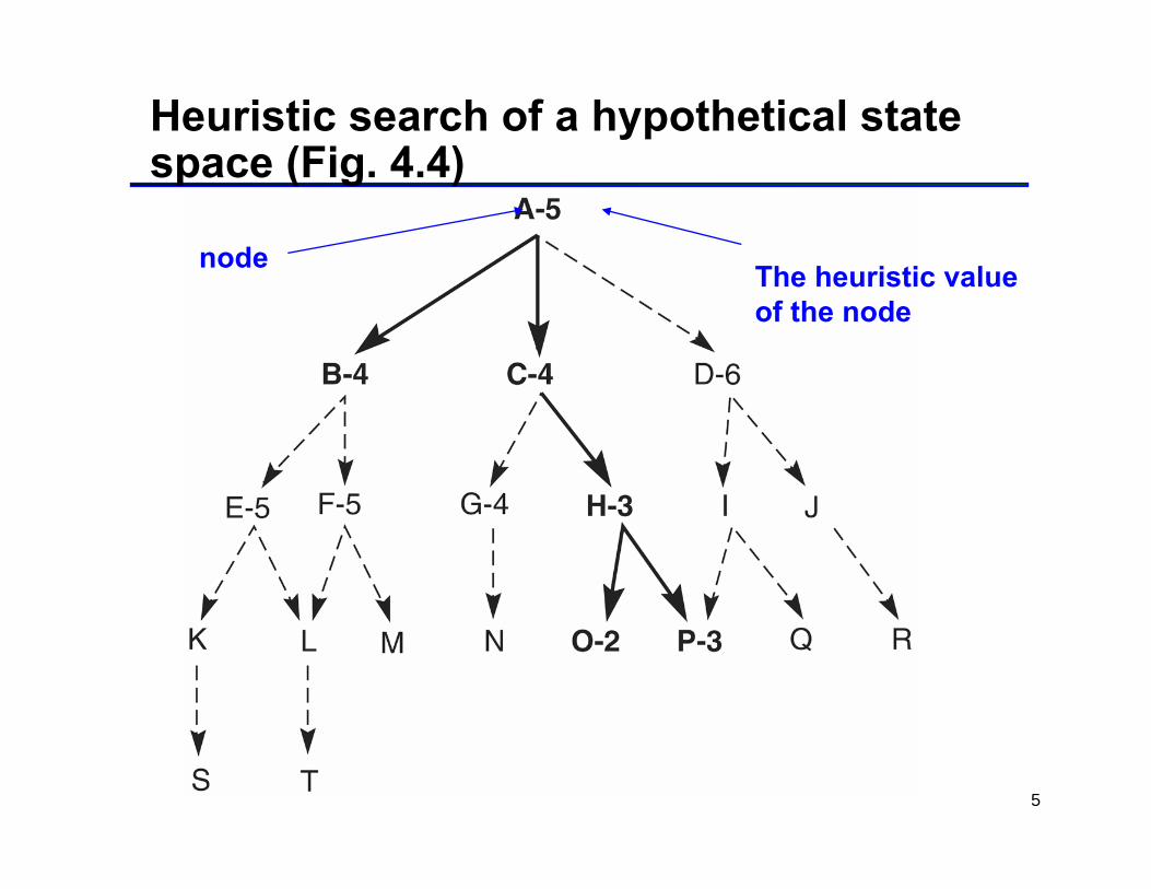
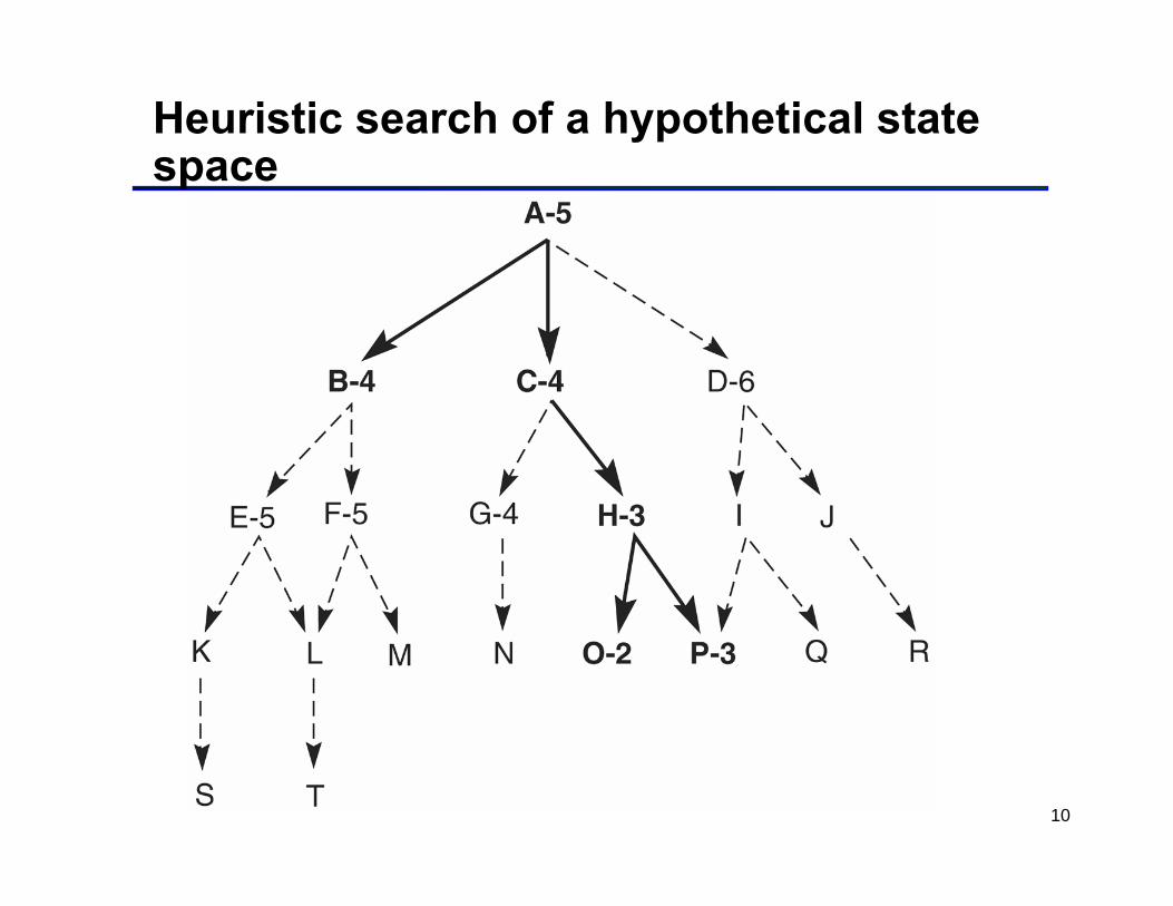
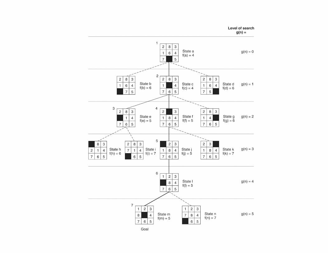
Heuristic search of a hypothetical state space (Fig. 4.4)

node The heuristic value of the node

6

Take the DFS algorithmFunction depth_first_search;

beginopen := [Start];closed := [ ];while open ≠ [ ] do

beginremove leftmost state from open, call it X;if X is a goal then return SUCCESS

else begingenerate children of X;put X on closed;discard remaining children of X if already on open or closedput remaining children on left end of open

endend;

return FAILend.

7

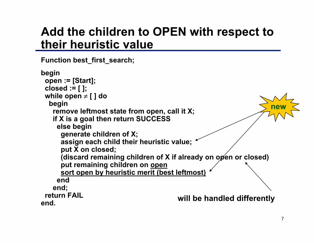
Add the children to OPEN with respect to their heuristic valueFunction best_first_search;

beginopen := [Start];closed := [ ];while open ≠ [ ] do

beginremove leftmost state from open, call it X;if X is a goal then return SUCCESS

else begingenerate children of X;assign each child their heuristic value;put X on closed;(discard remaining children of X if already on open or closed)put remaining children on opensort open by heuristic merit (best leftmost)

endend;

return FAILend.

new

will be handled differently

8

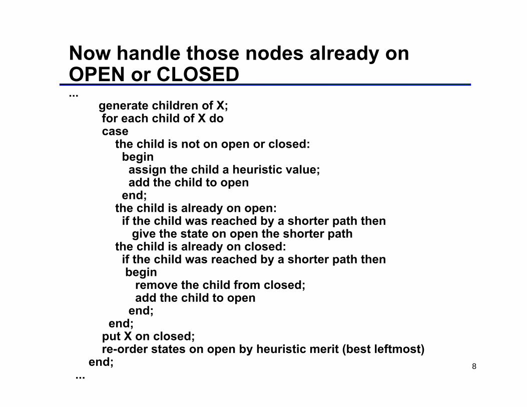
Now handle those nodes already on OPEN or CLOSED...

generate children of X;for each child of X docase

the child is not on open or closed:beginassign the child a heuristic value;add the child to open

end;the child is already on open:

if the child was reached by a shorter path thengive the state on open the shorter path

the child is already on closed:if the child was reached by a shorter path thenbegin

remove the child from closed;add the child to open

end;end;

put X on closed;re-order states on open by heuristic merit (best leftmost)

end;...

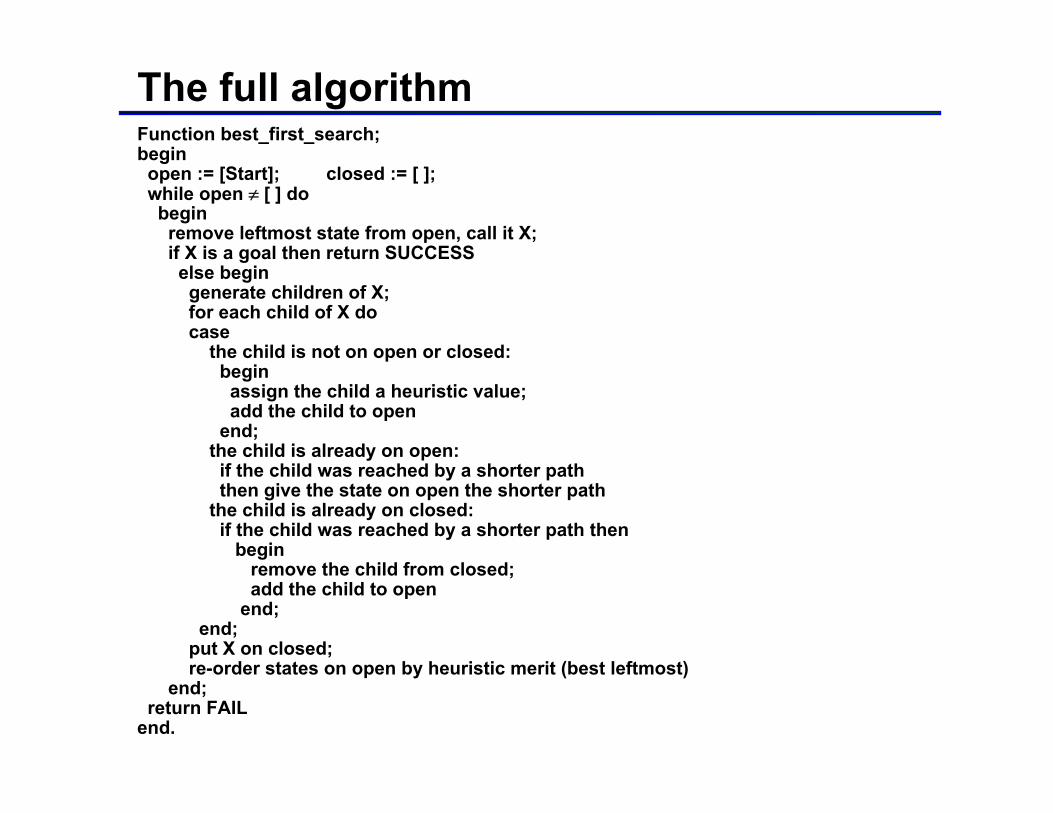
The full algorithmFunction best_first_search;begin

open := [Start]; closed := [ ];while open ≠ [ ] dobegin

remove leftmost state from open, call it X;if X is a goal then return SUCCESSelse begin

generate children of X;for each child of X docase

the child is not on open or closed:beginassign the child a heuristic value;add the child to open

end;the child is already on open:

if the child was reached by a shorter paththen give the state on open the shorter path

the child is already on closed:if the child was reached by a shorter path then

beginremove the child from closed;add the child to open

end;end;

put X on closed;re-order states on open by heuristic merit (best leftmost)

end;return FAIL

end.

10

Heuristic search of a hypothetical state space

11

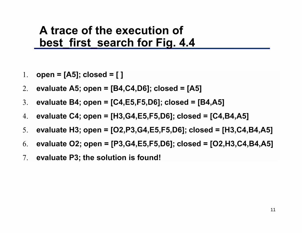
A trace of the execution of best_first_search for Fig. 4.4

12

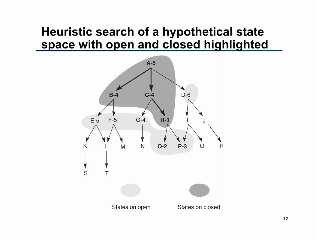
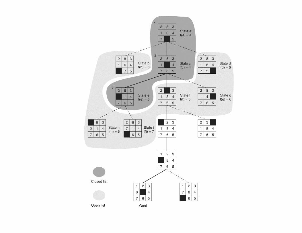
Heuristic search of a hypothetical state space with open and closed highlighted

13

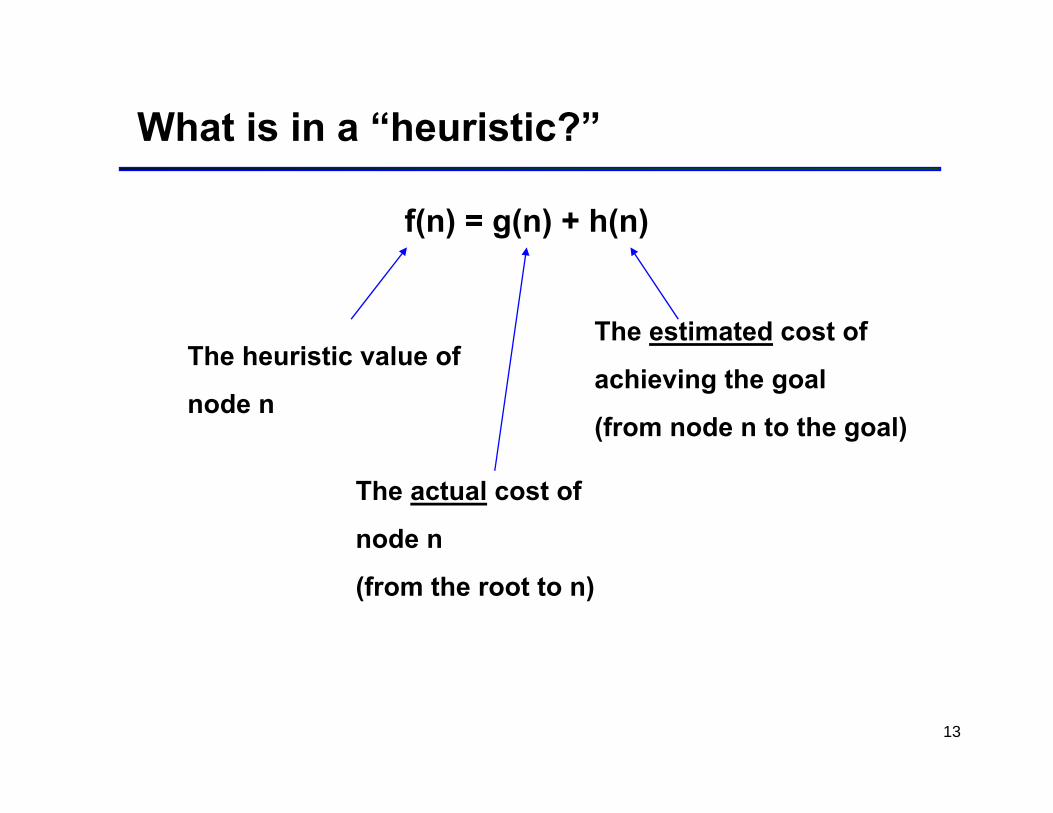
What is in a “heuristic?”

f(n) = g(n) + h(n)

The heuristic value of

node n

The actual cost of

node n

(from the root to n)

The estimated cost of

achieving the goal

(from node n to the goal)

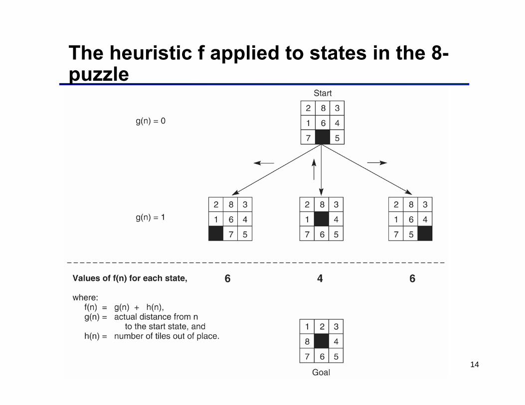
14

The heuristic f applied to states in the 8-puzzle

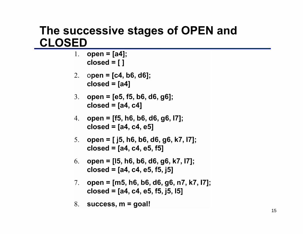
15

The successive stages of OPEN and CLOSED

18

Algorithm A

Consider the evaluation function f(n) = g(n) + h(n) where

n is any state encountered during the searchg(n) is the cost of n from the start stateh(n) is the heuristic estimate of the distance n to the goal

If this evaluation algorithm is used with the best_first_search algorithm of Section 4.1, the result is called algorithm A.

19

Algorithm A*

If the heuristic function used with algorithm A is admissible, the result is called algorithm A* (pronounced A-star).

A heuristic is admissible if it never overestimates the cost to the goal.

The A* algorithm always finds the optimal solution path whenever a path from the start to a goal state exists (the proof is omitted, optimality is a consequence of admissability).

20

Monotonicity

A heuristic function h is monotone if

1. For all states ni and nJ, where nJ is a descendant of ni,

h(ni) - h(nJ) ≤ cost (ni, nJ),

where cost (ni, nJ) is the actual cost (in number of moves) of going from state ni tonJ.

2. The heuristic evaluation of the goal state iszero, or h(Goal) = 0.

21

Informedness

For two A* heuristics h1 and h2, if h1 (n) ≤ h2 (n), for all states n in the search space, heuristic h2 is said to be more informed than h1.

23

Game playing

Games have always been an important application area for heuristic algorithms. The games that we will look at in this course will be two-person board games such as Tic-tac-toe, Chess, or Go.

24

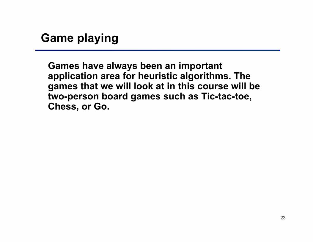
First three levels of tic-tac-toe state space reduced by symmetry

25

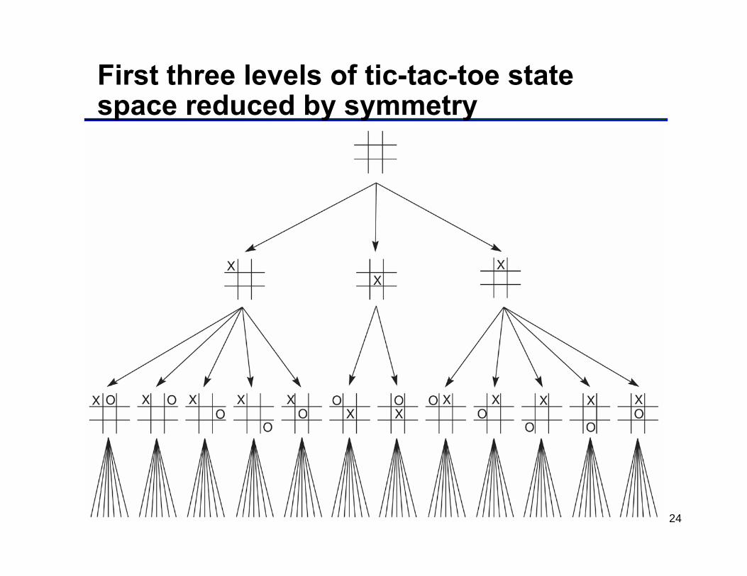
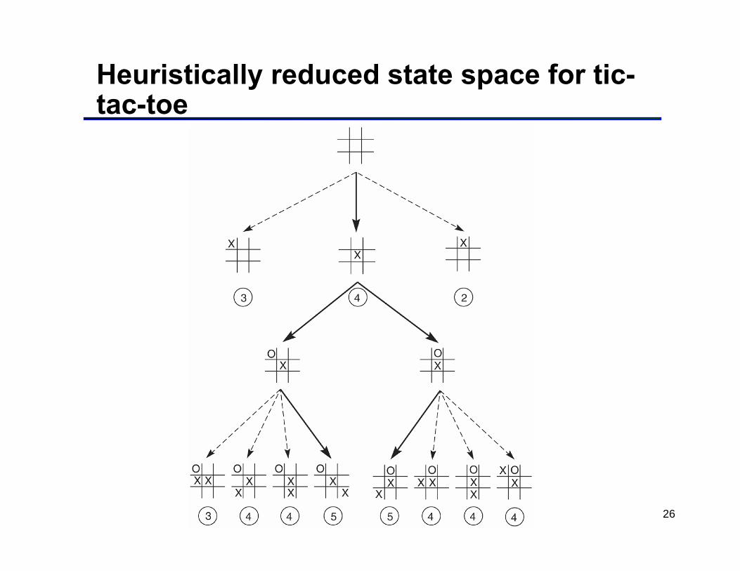
The “most wins” heuristic

26

Heuristically reduced state space for tic-tac-toe

27

A variant of the game nim

• A number of tokens are placed on a table between the two opponents

• A move consists of dividing a pile of tokens into two nonempty piles of different sizes

• For example, 6 tokens can be divided into piles of 5 and 1 or 4 and 2, but not 3 and 3

• The first player who can no longer make a move loses the game

• For a reasonable number of tokens, the state space can be exhaustively searched

28

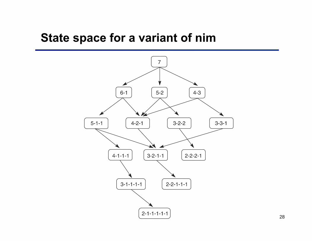
State space for a variant of nim

29

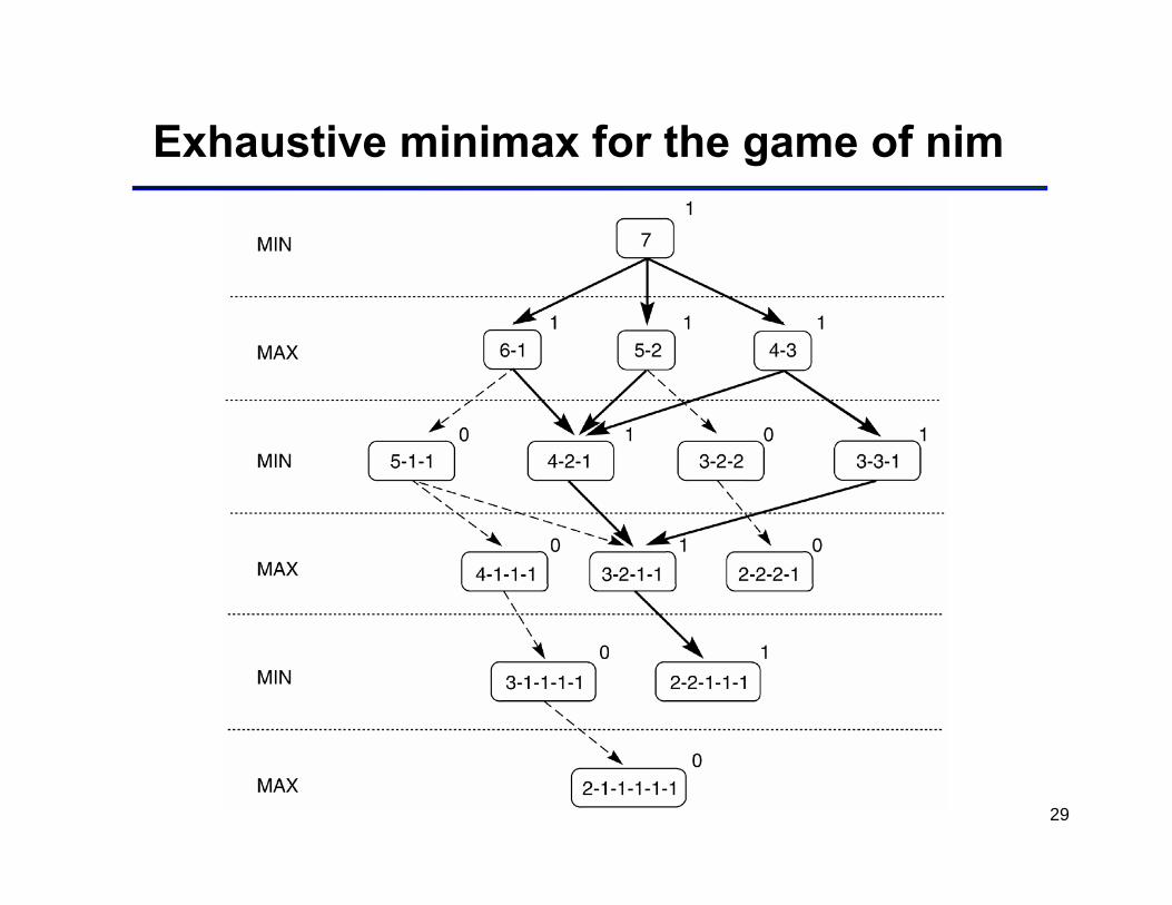
Exhaustive minimax for the game of nim

30

Two people games

• One of the earliest AI applications

• Several programs that compete with the best human players:

• Checkers: beat the human world champion• Chess: beat the human world champion (in 2002 & 2003)• Backgammon: at the level of the top handful of humans• Go: no competitive programs• Othello: good programs• Hex: good programs

31

Search techniques for 2-person games

• The search tree is slightly different: It is a two-ply tree where levels alternate between players

• Canonically, the first level is “us” or the player whom we want to win.

• Each final position is assigned a payoff:• win (say, 1)• lose (say, -1)• draw (say, 0)

• We would like to maximize the payoff for the first player, hence the names MAX & MINIMAX

32

The search algorithm

• The root of the tree is the current board position, it is MAX’s turn to play

• MAX generates the tree as much as it can, and picks the best move assuming that Min will also choose the moves for herself.

• This is the Minimax algorithm which was invented by Von Neumann and Morgenstern in 1944, as part of game theory.

• The same problem with other search trees: the tree grows very quickly, exhaustive search is usually impossible.

33

Special technique 1

• MAX generates the full search tree (up to the leaves or terminal nodes or final game positions) and chooses the best one:

win or tie• To choose the best move, values are propogated upward from the leaves:

• MAX chooses the maximum• MIN chooses the minimum

• This assumes that the full tree is not prohibitively big• It also assumes that the final positions are easily identifiable• We can make these assumptions for now, so let’s look at an example

34

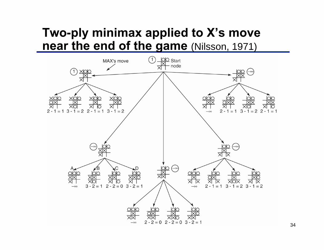
Two-ply minimax applied to X’s move near the end of the game (Nilsson, 1971)

35

Special technique 2• Notice that the tree was not generated to full depth in the previous example

• When time or space is tight, we can’t search exhaustively so we need to implement a cut-off point and simply not expand the tree below the nodes who are at the cut-off level.

• But now the leaf nodes are not final positions but we still need to evaluate them:

use heuristics

• We can use a variant of the “most wins” heuristic

36

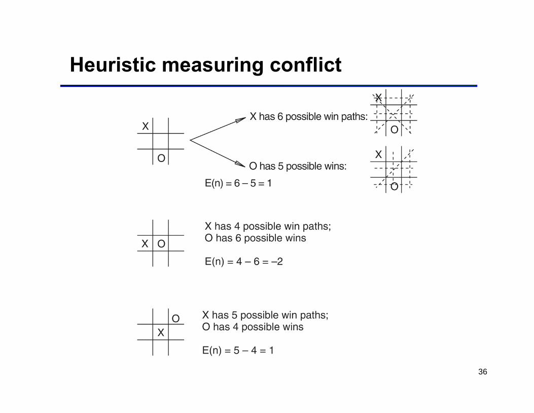
Heuristic measuring conflict

37

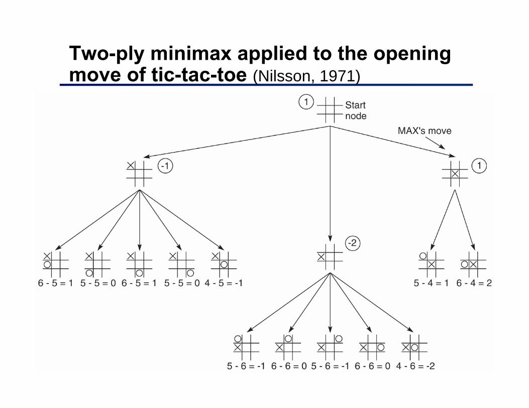
Calculation of the heuristic

• E(n) = M(n) – O(n) where• M(n) is the total of My (MAX) possible winning lines• O(n) is the total of Opponent’s (MIN) possible winning

lines• E(n) is the total evaluation for state n

• Take another look at the previous example

• Also look at the next two examples which use a cut-off level (a.k.a. search horizon) of 2 levels

38

Two-ply minimax applied to the opening move of tic-tac-toe (Nilsson, 1971)

39

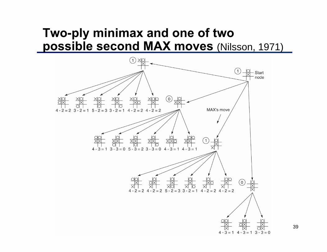
Two-ply minimax and one of two possible second MAX moves (Nilsson, 1971)

40

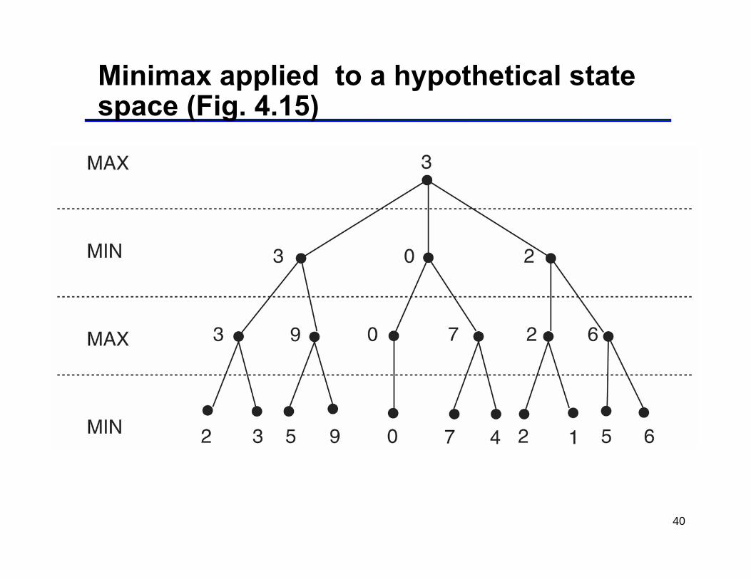
Minimax applied to a hypothetical state space (Fig. 4.15)

41

Special technique 3

• Use alpha-beta pruning

• Basic idea: if a portion of the tree is obviously good (bad) don’t explore further to see how terrific (awful) it is

• Remember that the values are propagated upward. Highest value is selected at MAX’slevel, lowest value is selected at MIN’s level

• Call the values at MAX levels α values, and the values at MIN levels β values

42

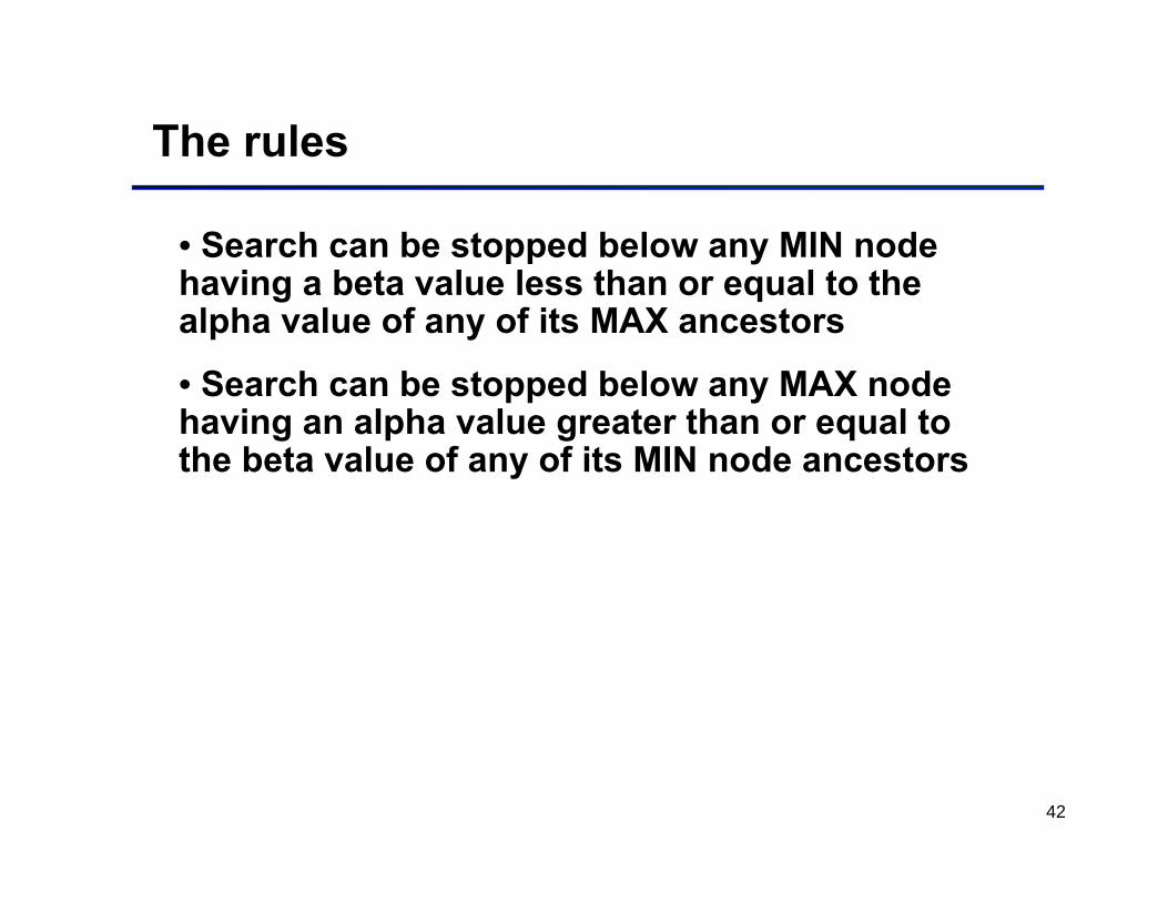
The rules

• Search can be stopped below any MIN node having a beta value less than or equal to the alpha value of any of its MAX ancestors

• Search can be stopped below any MAX node having an alpha value greater than or equal to the beta value of any of its MIN node ancestors

43

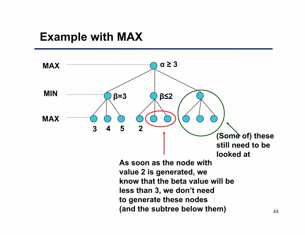
Example with MAX

MAX

MAX

MIN

3 4 5

β=3 β≤2

2

As soon as the node withvalue 2 is generated, we know that the beta value will be less than 3, we don’t needto generate these nodes (and the subtree below them)

α ≥ 3

(Some of) thesestill need to belooked at

44

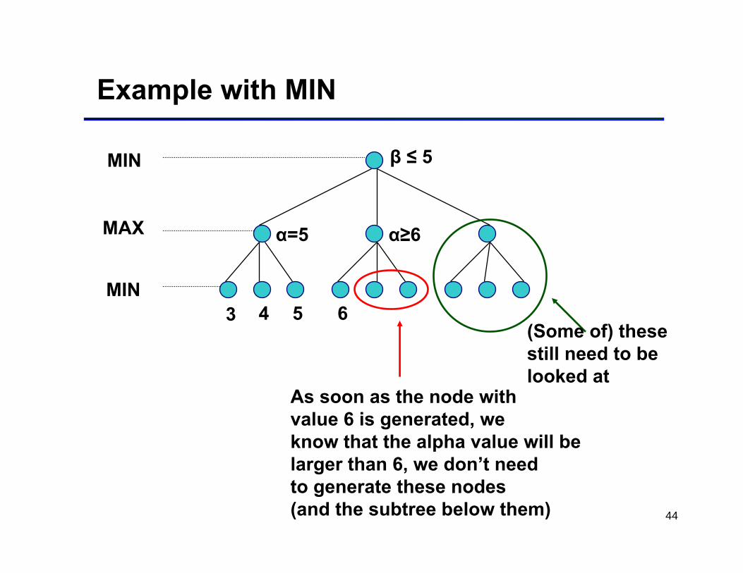
Example with MIN

MIN

MIN

MAX

3 4 5

α=5 α≥6

6

As soon as the node withvalue 6 is generated, we know that the alpha value will be larger than 6, we don’t needto generate these nodes (and the subtree below them)

β ≤ 5

(Some of) thesestill need to belooked at

45

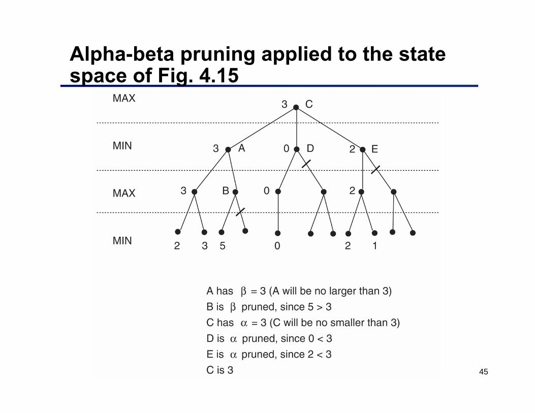
Alpha-beta pruning applied to the state space of Fig. 4.15

46

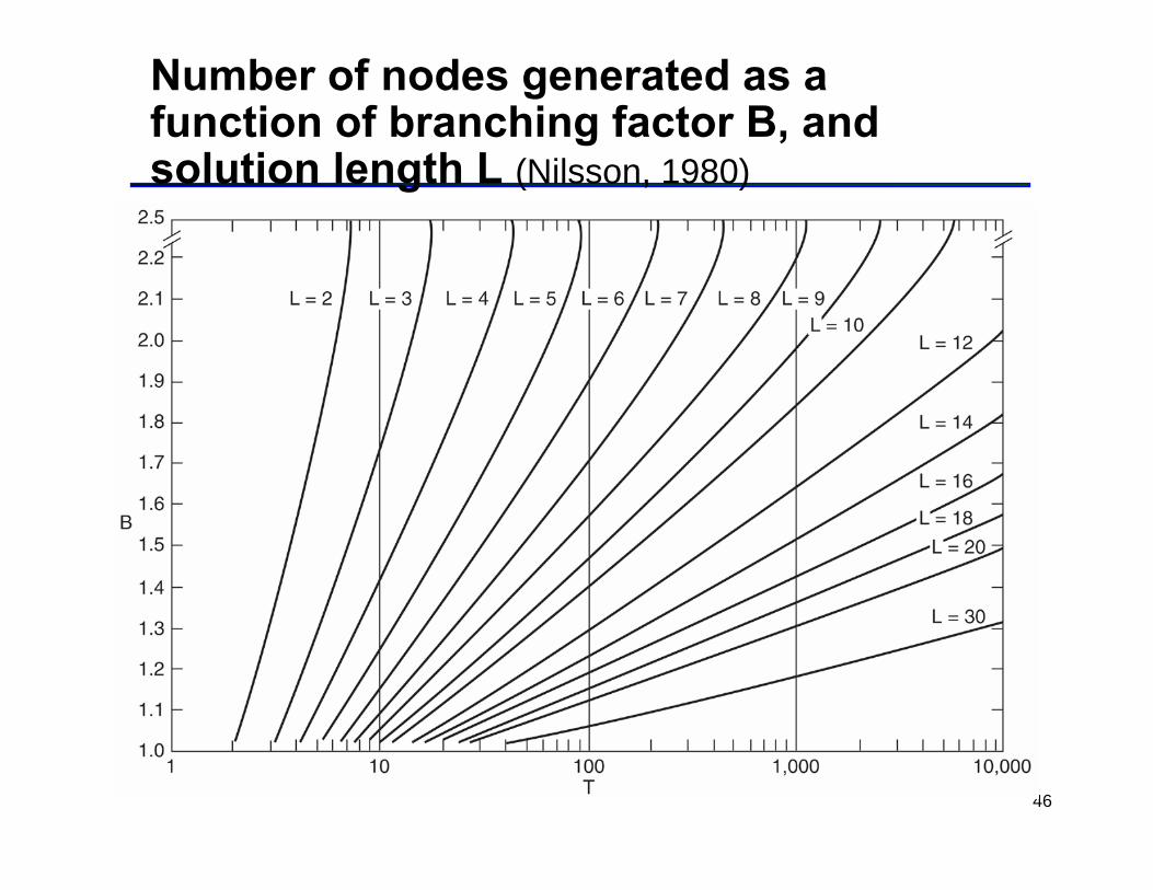
Number of nodes generated as a function of branching factor B, and solution length L (Nilsson, 1980)

47

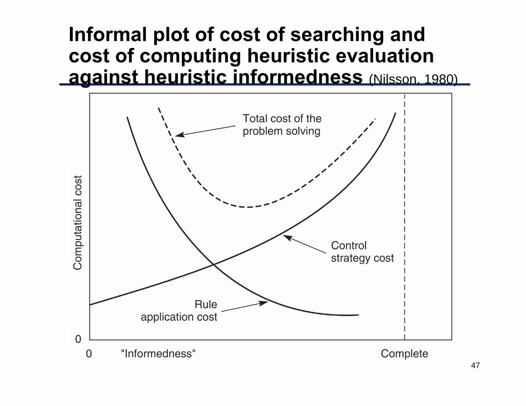
Informal plot of cost of searching and cost of computing heuristic evaluation against heuristic informedness (Nilsson, 1980)

48

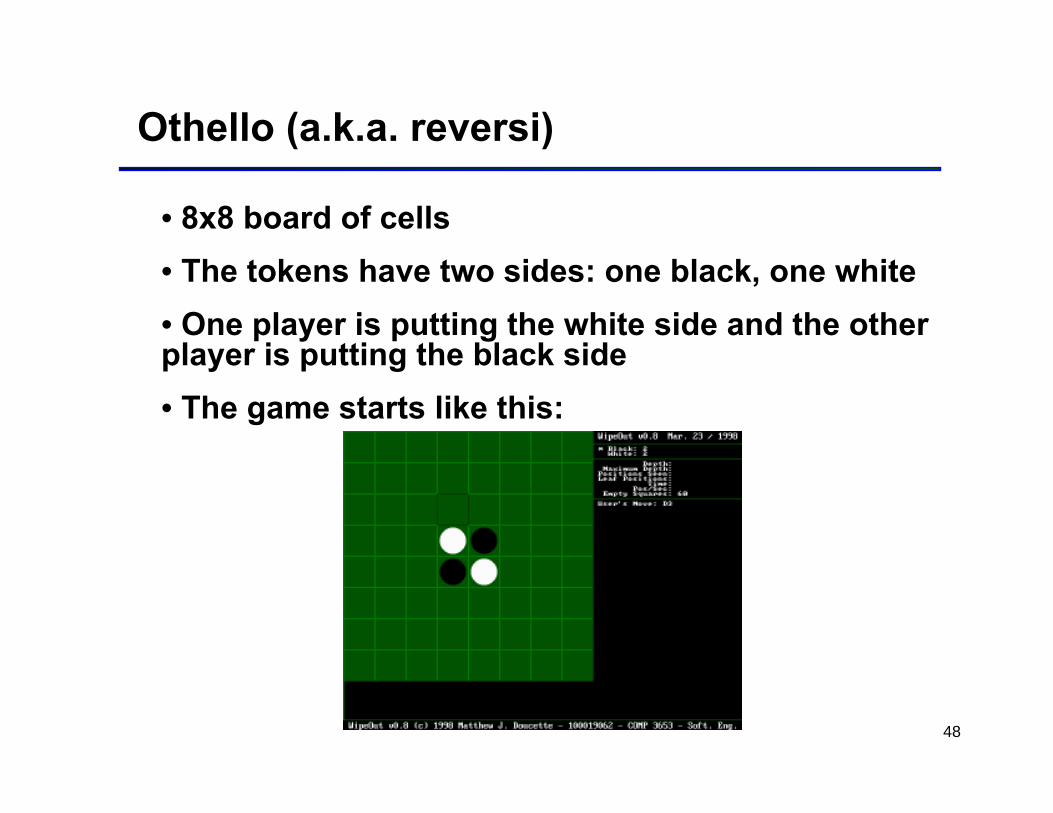
Othello (a.k.a. reversi)

• 8x8 board of cells• The tokens have two sides: one black, one white• One player is putting the white side and the other player is putting the black side• The game starts like this:

49

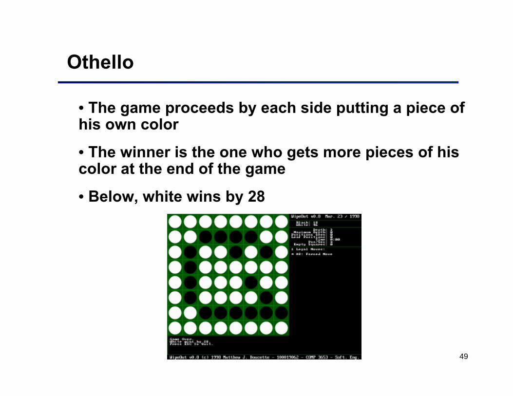
Othello

• The game proceeds by each side putting a piece of his own color

• The winner is the one who gets more pieces of his color at the end of the game

• Below, white wins by 28

50

Othello

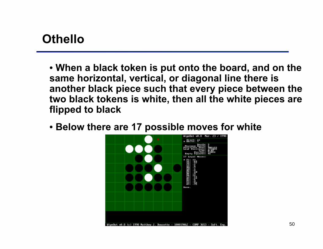
• When a black token is put onto the board, and on the same horizontal, vertical, or diagonal line there is another black piece such that every piece between the two black tokens is white, then all the white pieces are flipped to black

• Below there are 17 possible moves for white

51

Othello

• A move can only be made if it causes flipping of pieces. A player can pass a move iff there is no move that causes flipping. The game ends when neither player can make a move• the snapshots are from www.mathewdoucette.com/artificialintelligence

• the description is fromhome.kkto.org:9673/courses/ai-xhtml• AAAI has a nice repository: www.aaai.orgClick on AI topics, then select “games & puzzles”from the menu

52

Hex

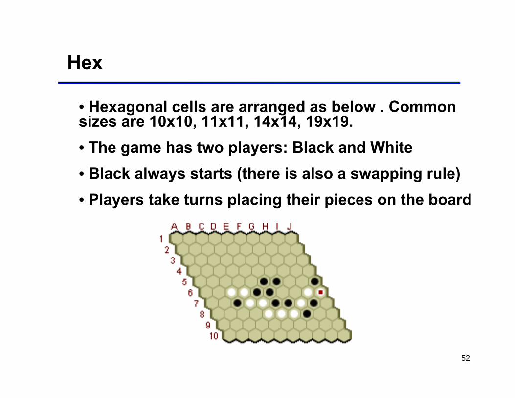
• Hexagonal cells are arranged as below . Common sizes are 10x10, 11x11, 14x14, 19x19.• The game has two players: Black and White• Black always starts (there is also a swapping rule)• Players take turns placing their pieces on the board

53

Hex

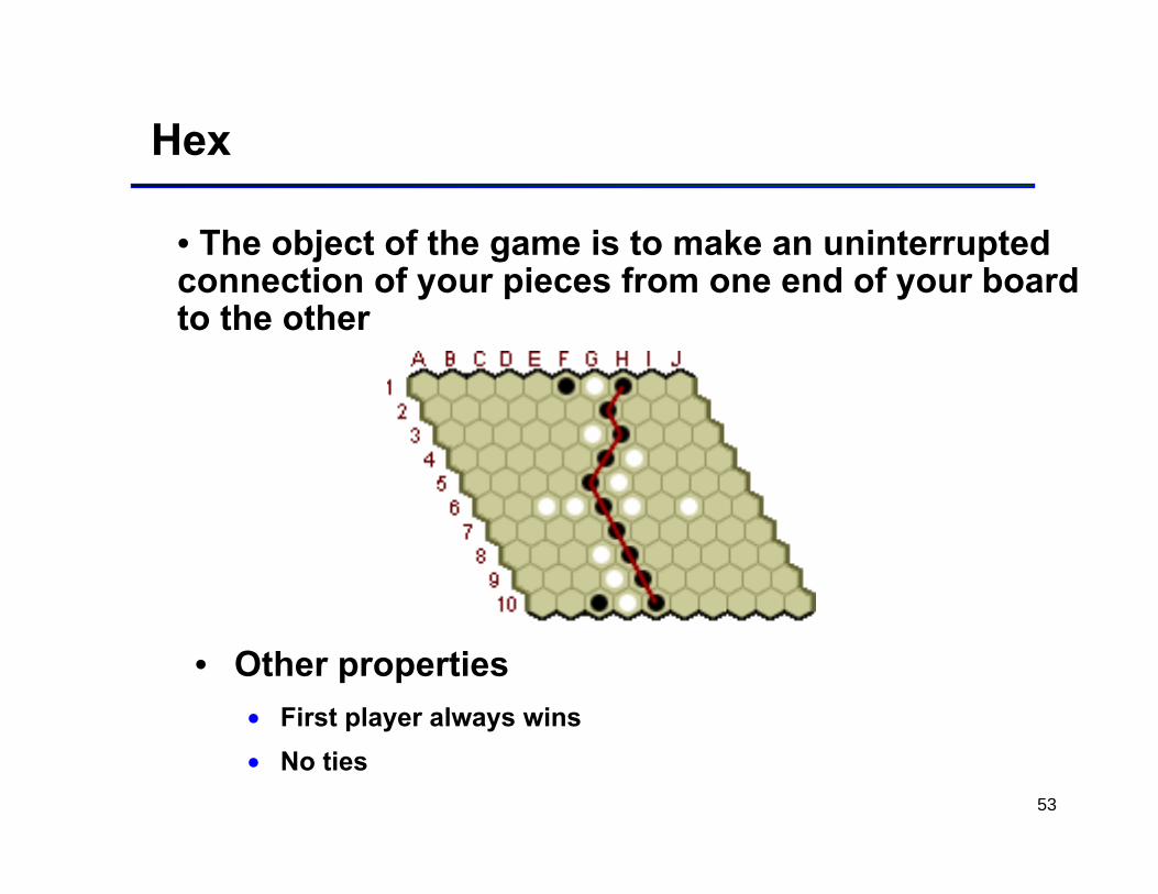
• The object of the game is to make an uninterrupted connection of your pieces from one end of your board to the other

• Other properties• First player always wins• No ties

54

•Hex

• Invented independently by Piet Hein in 1942 and John Nash in 1948.

• Every empty cell is a legal move, thus the game tree is wide b = ~80 (chess b = ~35, go b = ~250)

• Determining the winner (assuming perfect play) in an arbitrary Hex position is PSPACE-complete [Rei81].

• How to get knowledge about the “potential” of a given position without massive game-tree search?

55

Hex

• There are good programs that play with heuristics to evaluate game configurations

• hex.retes.hu/six

• home.earthlink.net/~vanshel

• cs.ualberta.ca/~javhar/hex

• www.playsite.com/t/games/board/hex/rules.html

56

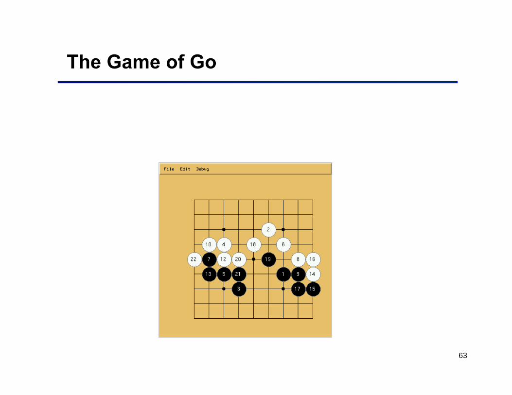
The Game of Go

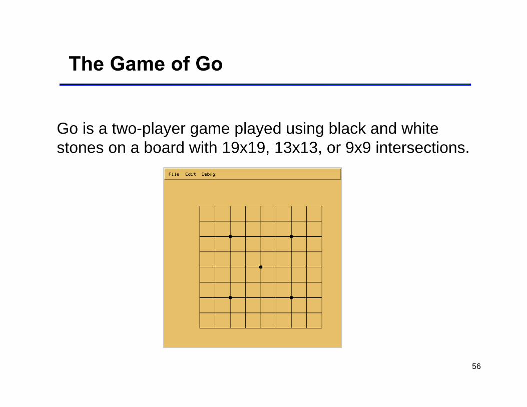
Go is a two-player game played using black and white stones on a board with 19x19, 13x13, or 9x9 intersections.

57

The Game of Go

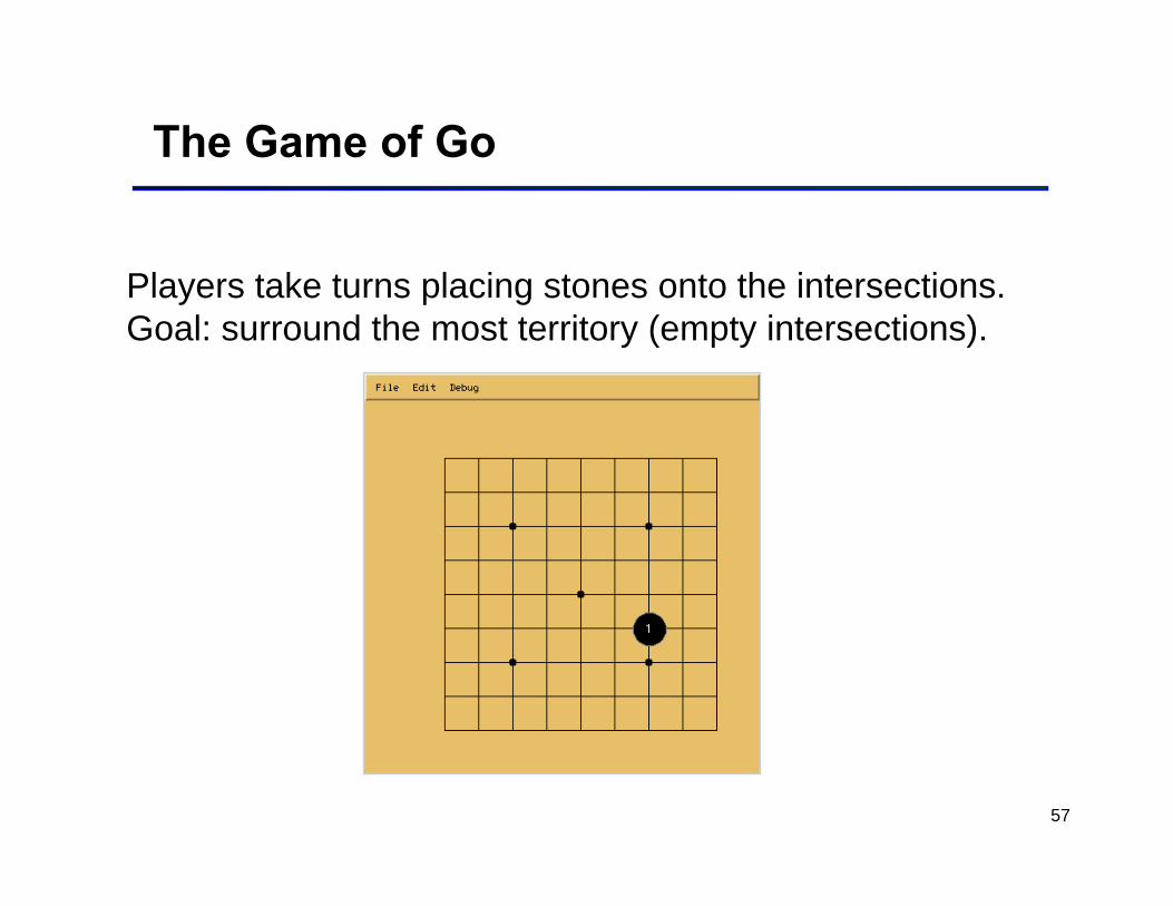
Players take turns placing stones onto the intersections. Goal: surround the most territory (empty intersections).

58

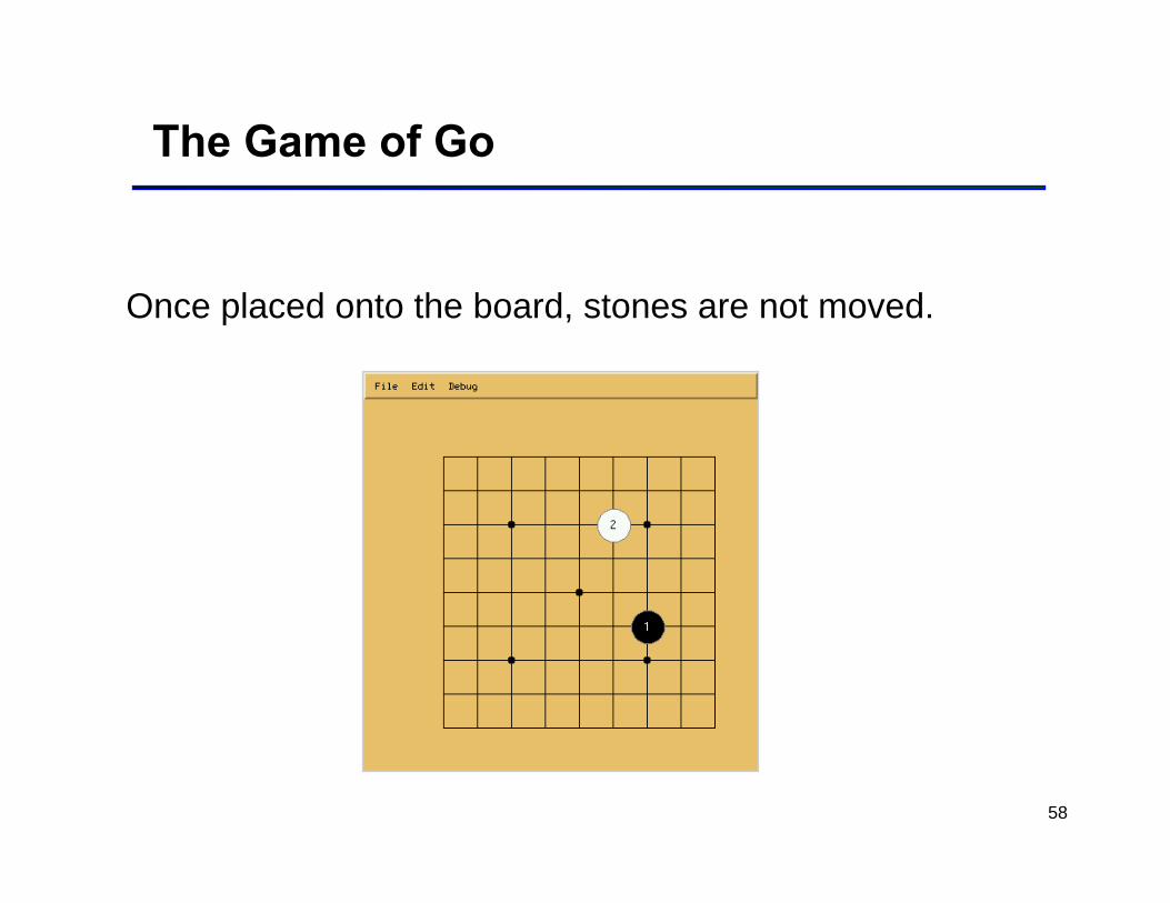
The Game of Go

Once placed onto the board, stones are not moved.

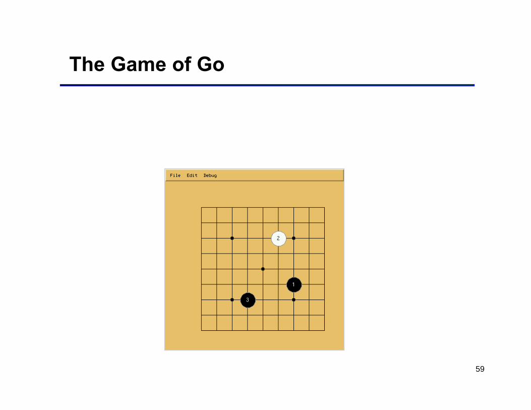
59

The Game of Go

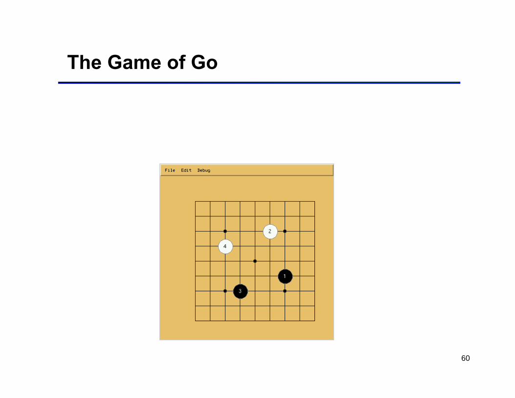
60

The Game of Go

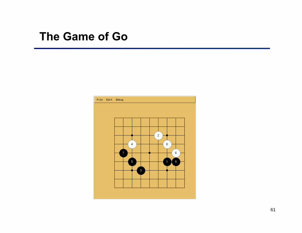
61

The Game of Go

62

The Game of Go

63

The Game of Go

64

The Game of Go

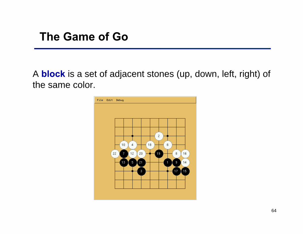
A block is a set of adjacent stones (up, down, left, right) of the same color.

65

The Game of Go

A block is a set of adjacent stones (up, down, left, right) of the same color.

66

The Game of Go

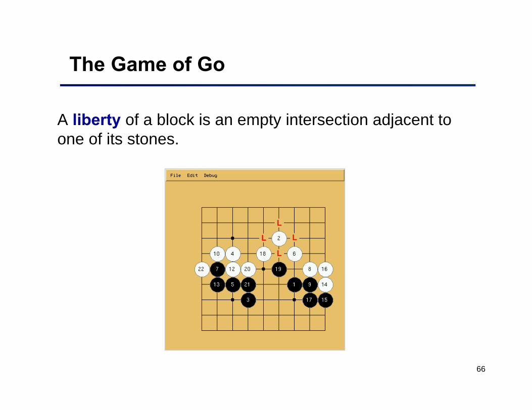
A liberty of a block is an empty intersection adjacent to one of its stones.

67

The Game of Go

68

The Game of Go

69

The Game of Go

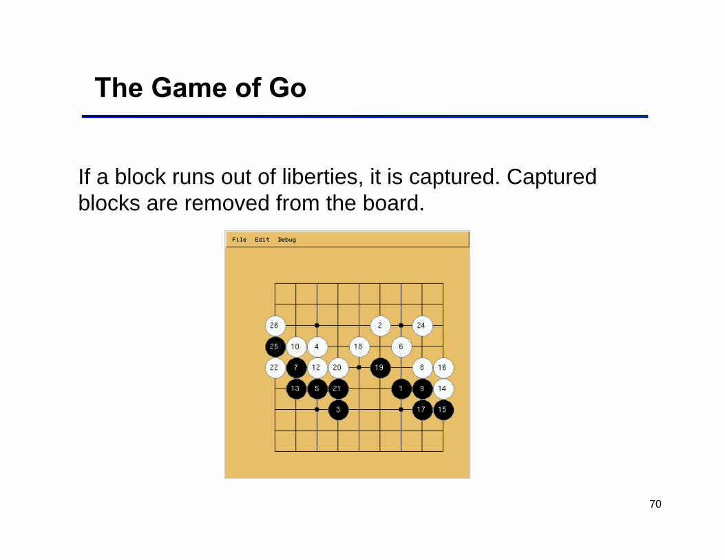
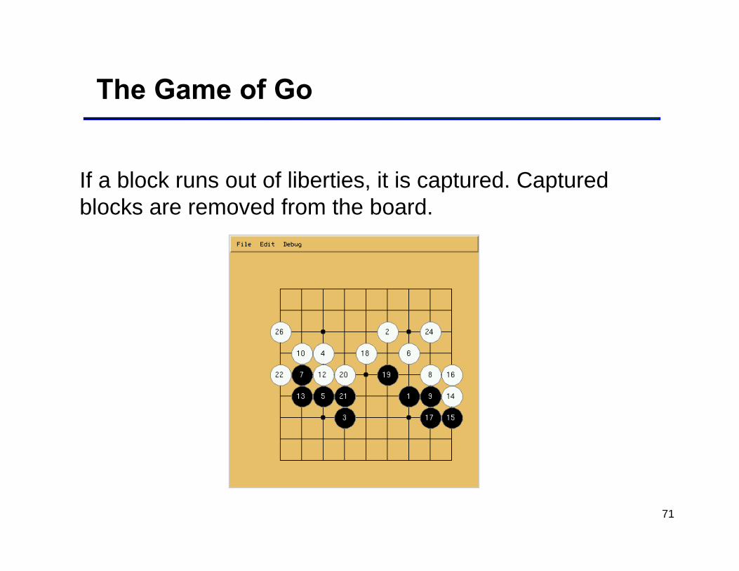
If a block runs out of liberties, it is captured. Captured blocks are removed from the board.

70

The Game of Go

If a block runs out of liberties, it is captured. Captured blocks are removed from the board.

71

The Game of Go

If a block runs out of liberties, it is captured. Captured blocks are removed from the board.

72

The Game of Go

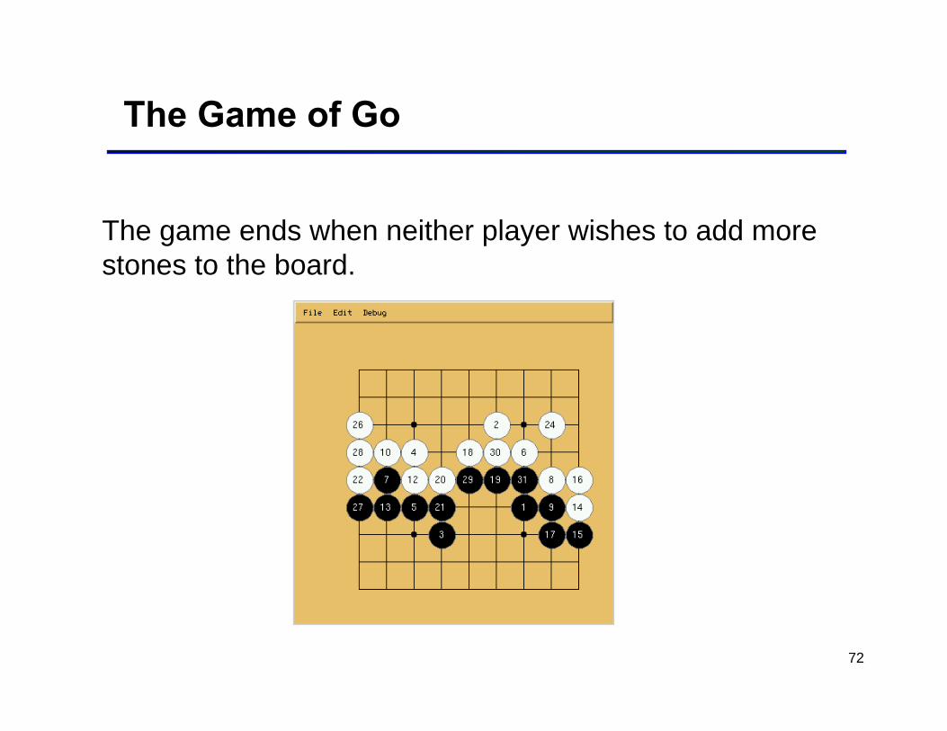
The game ends when neither player wishes to add more stones to the board.

73

The Game of Go

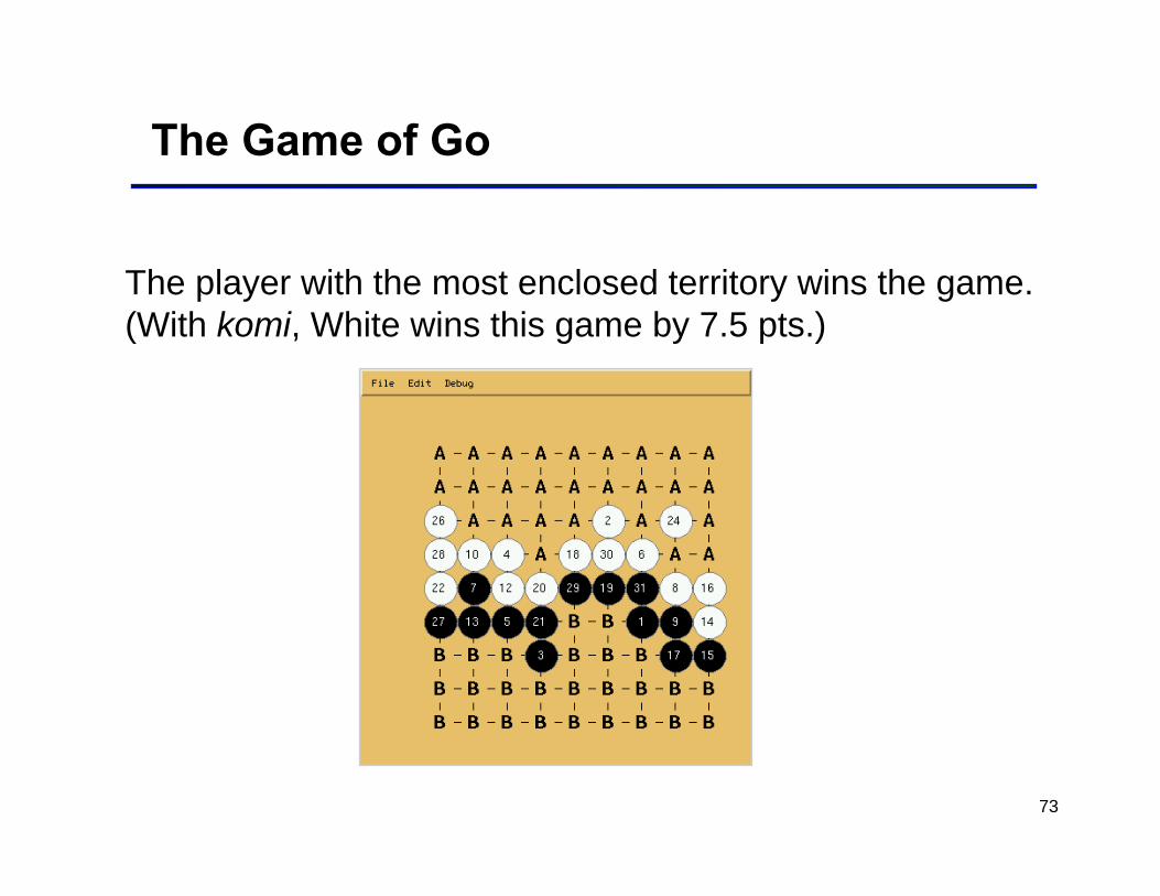
The player with the most enclosed territory wins the game. (With komi, White wins this game by 7.5 pts.)

74

Alive and Dead Blocks

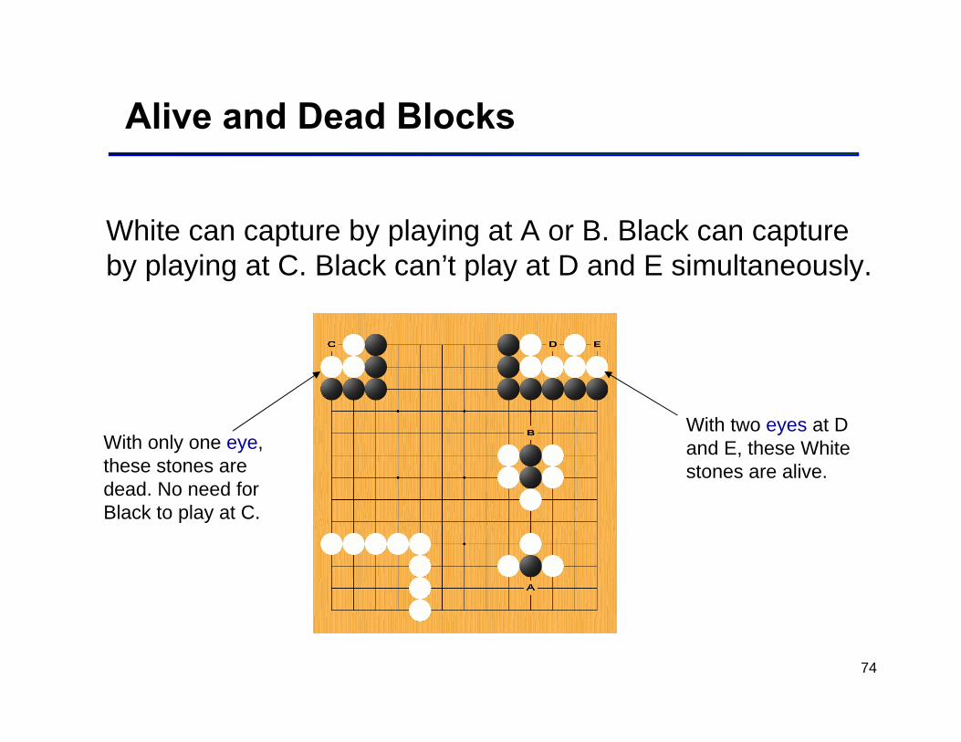
White can capture by playing at A or B. Black can capture by playing at C. Black can’t play at D and E simultaneously.

With only one eye, these stones are dead. No need for Black to play at C.

With two eyes at D and E, these White stones are alive.

75

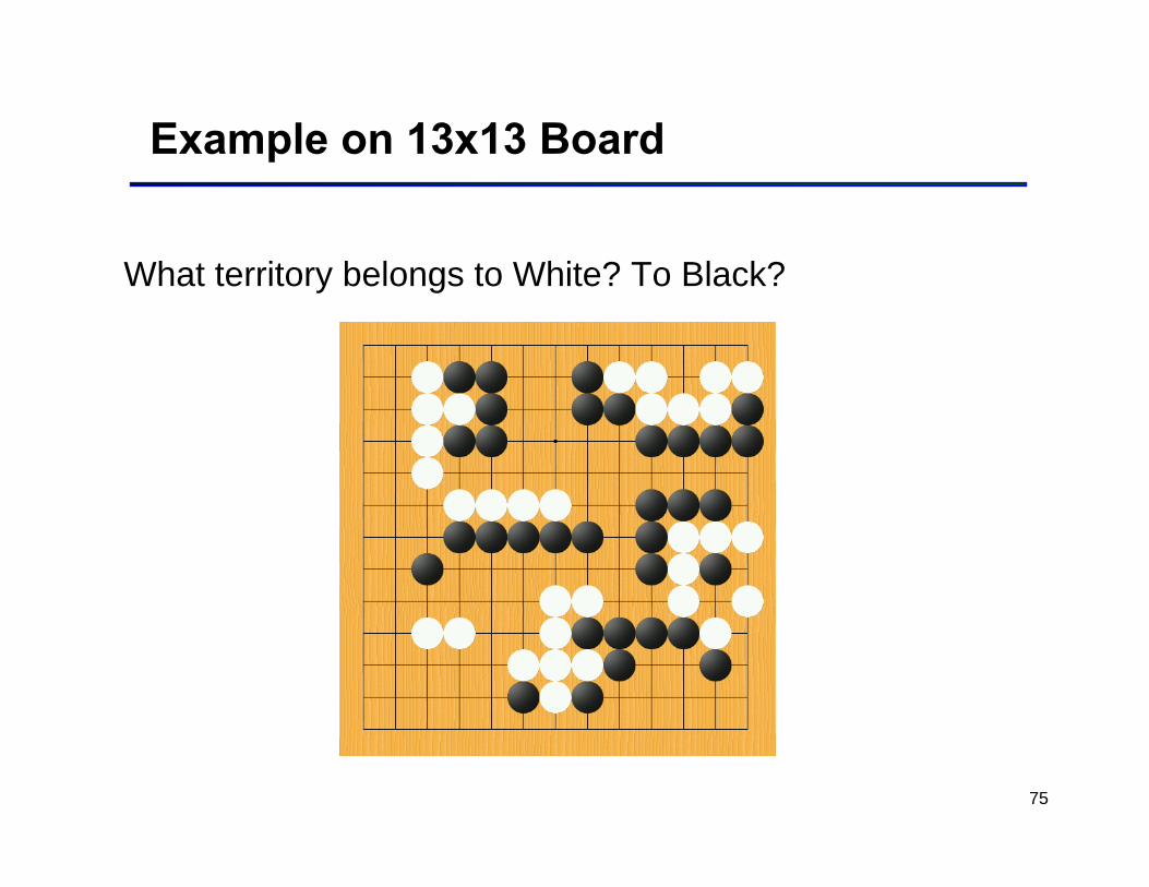
Example on 13x13 Board

What territory belongs to White? To Black?

76

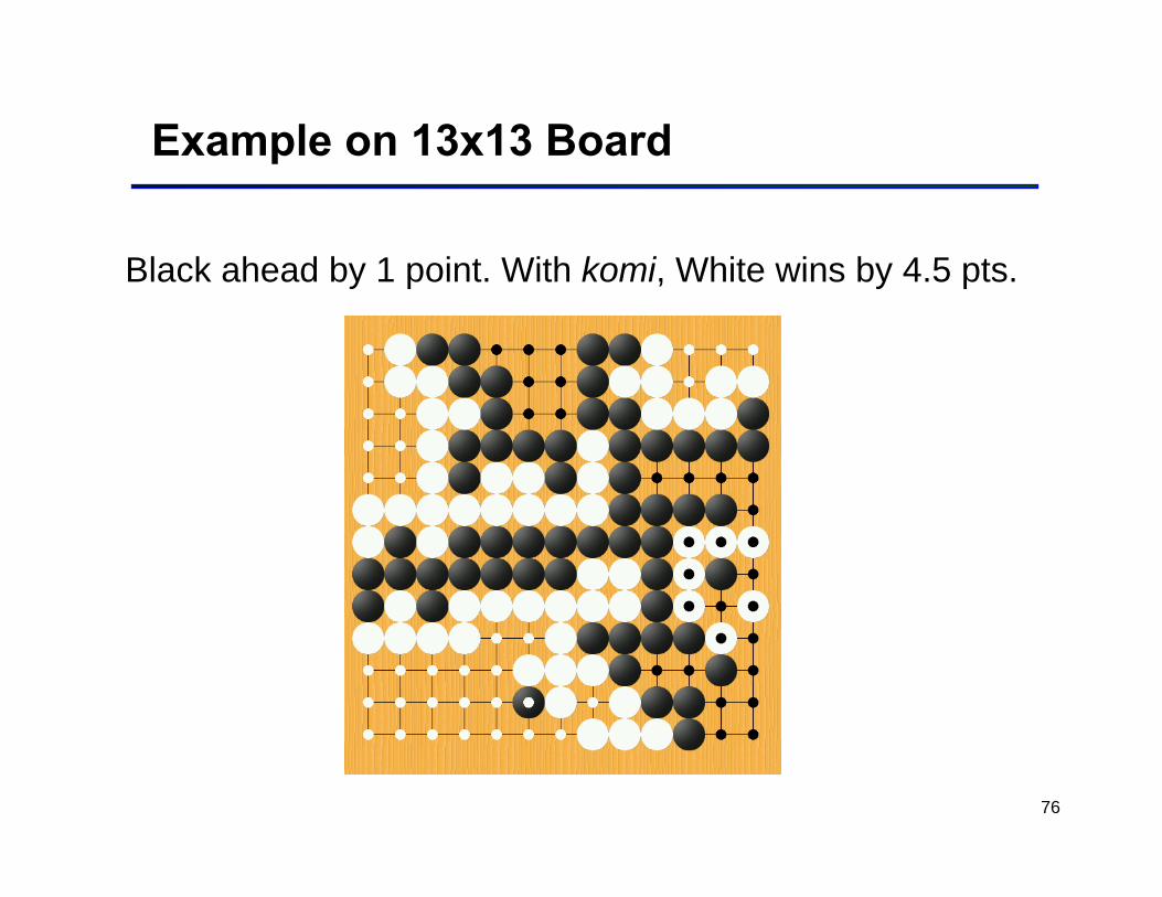
Example on 13x13 Board

Black ahead by 1 point. With komi, White wins by 4.5 pts.

77

Challenges for Computer Go

Much higher search requirements• Minimax game tree has O(bd) positions• In chess, b = ~35 and d = ~100 half-moves• In Go, b = ~250 and d = ~200 half-moves• However, 9x9 Go seems almost as hard as 19x19

Accurate evaluation functions are difficult to build and computationally expensive• In chess, material difference alone works fairly well• In Go, only 1 piece type with no easily extracted features

Determining the winner from an arbitrary position is PSPACE-hard (Lichtenstein and Sipser, 1980)

78

State of the Art

Many Faces of Go v.11 (Fotland), Go4++ (Reiss), Handtalk/Goemate (Chen), GNUGo (many), etc.

Each consists of a carefully crafted combination of pattern matchers, expert rules, and selective search

Playing style of current programs:• Focus on safe territories and large frameworks • Avoid complicated fighting situations

Rank is about 6 kyu, though actual playing strength varies from opening (stronger) to middle game (much weaker) to endgame (stronger)