4. Face & Iris Recognition - Shodhgangashodhganga.inflibnet.ac.in/bitstream/10603/9044/9/09_chapter...

149

4. Face & Iris Recognition

Face as a biometric trait has universality and very low degree of

cooperation requirement, on the other hand though iris recognition

systems require elevated degree of cooperation from the user

accuracy is high. Both face and iris based biometric systems are

gaining popularity due to their use in surveillance and screening

systems at places like airports, bus & railway stations, public places

etc. Iris recognition systems are gaining importance due to its use

in electronic passports by various countries. In this chapter we

discuss different techniques based on image processing for face and

iris recognition.

4.1 Face Recognition

Among all biometrics listed previously, face belongs to both

physiological and behavioral categories. In addition face has

advantage over other biometrics because it is a natural, non-

intrusive, and easy-to-use biometric. Probably the most important

feature of a biometric is its ability to collect the signature from non-

cooperating subjects. Besides applications related to identification

and verification such as access control, law enforcement, ID and

licensing, surveillance etc., face recognition is also useful in human-

computer interaction, virtual reality, database retrieval, multimedia,

computer entertainment etc. Face recognition mainly involves the

following three tasks [229], [230]:

Verification - The recognition system determines if the query

face image and the claimed identity match.

Identification - The recognition system determines the

identity of the query face image by matching it with a

database of images with known identities, assuming that the

identity of the query face image is inside the database.

Watch list - The recognition system first determines if the

identity of the query face image is in the stored watch list and,

if yes, then identifies the individual.

We have implemented face recognition systems using Gabor

filter response of face image, LBG Clustering Algorithm, Kekre’s

Median Codebook Generation Algorithm (KMCG) & Kekre’s Fast

Codebook Generation (KFCG) based vector quantization is also

implemented for feature vector extraction. In another variation we

150

have implemented previously used Kekre’s Wavelet & Haar Wavelet

Energy Entropy based feature extraction for face recognition. We

now discuss these techniques in detail in the next sections.

4.1.1 Face Recognition using Gabor Filters

Many researchers have used Gabor filters for face recognition. As

the data generated in case of Gabor filter based approach is huge

dimensionality reduction techniques such as PCA, LDA Fischer

analysis are required to be used along with Gabor filter response.

This requires heavy processing power. Here we have developed a

system by using Gabor Filter response directly; such system [241]

is used by authors for Content Based Image Retrieval (CBIR).

Advantage of such system is less complexity & comparatively

reduced processing requirements suitable for handheld devices.

Handheld devices have less memory & computing power, small size

of feature vector and lesser computations make current system

suitable for handheld device such as PDA & Windows CE mobile

phone.

Gabor filters are bandpass filters which have both orientation-

selective and frequency-selective properties and have optimal joint

resolution in both spatial and frequency domains [193], [208],

[209]. We have used Gabor filters for segmentation of fingerprints

in Section 3.1.1.2. A Gabor filter has the following general form in

the spatial domain [193].

2 2

2 2

1h( , , , , , ) = exp{- } exp( 2 )

2

k k

kk x y

x y

x yx y f i fx

(4.1)

Where cos sink k kx x y , and sin cos

k k ky x y,

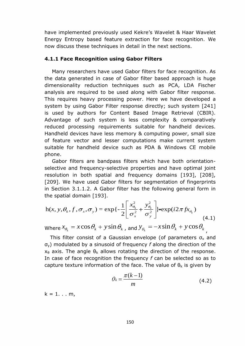
This filter consist of a Gaussian envelope (of parameters σx and

σy) modulated by a sinusoid of frequency f along the direction of the

xθ axis. The angle θk allows rotating the direction of the response.

In case of face recognition the frequency f can be selected so as to

capture texture information of the face. The value of θk is given by

( 1)

kk

m (4.2)

k = 1. . . m,

151

Where m denotes the number of orientations (Currently m = 8). For

each face image block of size W ×W centered at (X,Y), with W even,

we extract the Gabor Magnitude [207] as follows for k = 1, . . . ,m:

( / 2) 1 ( / 2) 1

0

/ 2 / 2

0 0 0

0 0

( , , , , , ) , ) ( , , , , , )| |(

W W

W W

k x y k x yx y

g X Y f X Y y h x y fI x

(4.3)

Where, I(x, y) denotes the gray level of the pixel (x, y) taken as

average of the R, G, B components of the image. As a result, we

obtain m Gabor features for each W ×W block of the image. In

blocks with high texture content, the values of one or several Gabor

features will be higher than the others (those values whose filter

angle is similar to the ridge angle of the block). If the block is noisy

or having non-oriented background, the m values of the Gabor

features will be similar. Therefore, the standard deviation ‘Sd’ of the

‘m’ Gabor features allows capturing of local texture information.

4.1.1.1 Gabor Filter Based Feature Vector Generation

We are using 8 Directions of the Gabor Filters (K=0 to 7), the

angle values are {θ = 0, 22.5, 45, 67.5, 90, 112.5, 135,157.5}. We

have selected the frequency by empirical study. The frequency

values are selected so as to capture maximum texture information

and give maximum matching.

(b) (c)

(a) (d) (e)

Fig. 4.1. Gabor Filter Standard Deviation Maps of an Input face Image (a)

Input face Image (b) f=4 Pixel/Cycle (c) f=8 Pixel/Cycle (d) f=10

Pixel/Cycle (e) f=12 Pixel/Cycle (f) Snapshot of Gabor Filter SD Values

for one Row (frequency = 4 Pixel/cycle).

152

We are using 4, 8, 10, 12 pixel/cycle as the frequency values. Input

Face image is selected and scaled to 256x256 pixels or the Face is

selected through a 256x256 window. Gaussian envelope (of

parameters σx and σy) are taken as σx = 4 and σy= 4. The block size

is 16X16 pixels (W x W).

For each frequency value we get 8 Gabor Filter Response arrays

of size 16 X 16, for each block 8 values of filter response are

available, we calculate standard deviations of these values as

discussed previously. For four different frequency values we get four

different arrays for standard deviation of Gabor filter response. Fig.

4.1 shows a typical face image and its corresponding Gabor Filter

Standard Deviation maps for four frequency values (4, 8, 10, and

12). This four standard deviation arrays are used as a feature

vectors for face. The steps for feature extraction are as listed below.

1. Read the face image, select the ROI. Scale the selected part

to 256X256 pixels size.

2. Divide the selected face into 16X16 pixels size blocks.

3. For each block find Gabor Filter response for four different

scales (frequency) of 4, 8, 10, 12 pixels/cycle and eight

different values of filter angle {θ = 0, 22.5, 45, 67.5, 90,

112.5, 135,157.5}. Store this response in a Multi-

dimensional array of size [Angle, Scale, Width/W, Height/W]

(Width=Height=256, W=16).

4. For each Scale find Standard Deviation Sd for Gabor Filter

response of 8 angles, We will get four different set of values

for four different scales. Store these values in a 3-D array of

size [Scale, Width/W, and Height/W]. For 8 Scales the typical

feature vector size is 8*16*16=1024 elements.

5. For each user account read ‘N’ training faces with different

poses or expressions. Repeat steps 1 to 5 for calculating

feature vector. Save this data on disk.

We are using K-Nearest Neighborhood (KNN) classifier to find

classifying faces & Euclidian Distance between two feature vectors

FV1(s, i, j) & FV2(s, i, j) is used for calculating matching distance.

3 1 12

1 2

0 0 0

Matching Distance ( ( , , ) ( ( , , ))w w

s i j

FV s i j FV s i j (4.4)

153

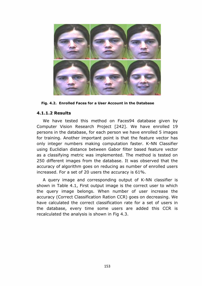
Fig. 4.2. Enrolled Faces for a User Account in the Database

4.1.1.2 Results

We have tested this method on Faces94 database given by

Computer Vision Research Project [242]. We have enrolled 19

persons in the database, for each person we have enrolled 5 images

for training. Another important point is that the feature vector has

only integer numbers making computation faster. K-NN Classifier

using Euclidian distance between Gabor filter based feature vector

as a classifying metric was implemented. The method is tested on

250 different images from the database. It was observed that the

accuracy of algorithm goes on reducing as number of enrolled users

increased. For a set of 20 users the accuracy is 61%.

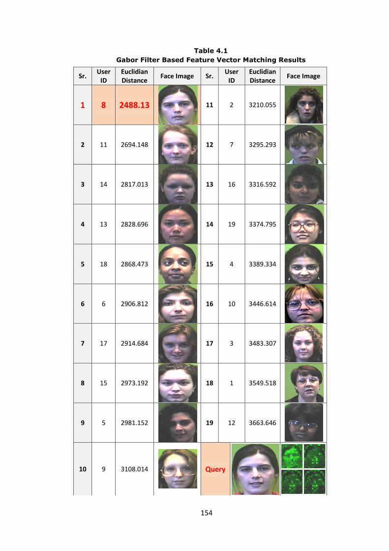
A query image and corresponding output of K-NN classifier is

shown in Table 4.1, First output image is the correct user to which

the query image belongs. When number of user increase the

accuracy (Correct Classification Ration CCR) goes on decreasing. We

have calculated the correct classification rate for a set of users in

the database, every time some users are added this CCR is

recalculated the analysis is shown in Fig 4.3.

154

Table 4.1

Gabor Filter Based Feature Vector Matching Results

Sr. User

ID Euclidian Distance

Face Image Sr. User

ID Euclidian Distance

Face Image

1 8 2488.13

11 2 3210.055

2 11 2694.148

12 7 3295.293

3 14 2817.013

13 16 3316.592

4 13 2828.696

14 19 3374.795

5 18 2868.473

15 4 3389.334

6 6 2906.812

16 10 3446.614

7 17 2914.684

17 3 3483.307

8 15 2973.192

18 1 3549.518

9 5 2981.152

19 12 3663.646

10 9 3108.014

Query

155

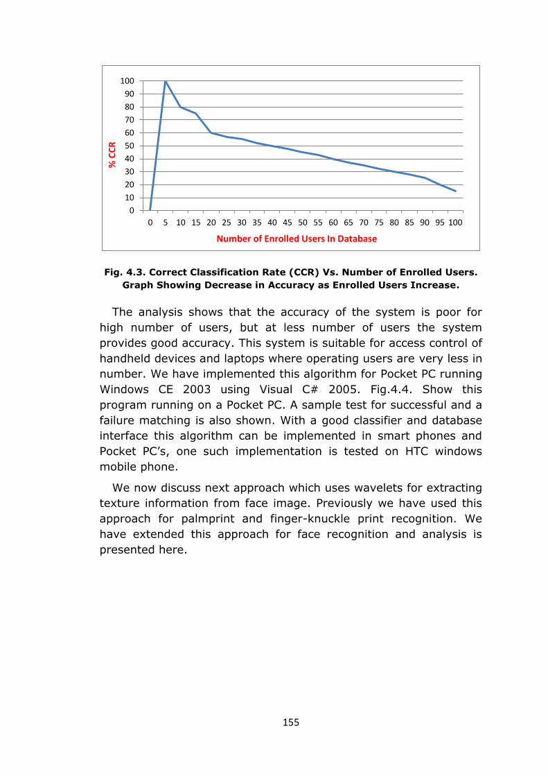
Fig. 4.3. Correct Classification Rate (CCR) Vs. Number of Enrolled Users.

Graph Showing Decrease in Accuracy as Enrolled Users Increase.

The analysis shows that the accuracy of the system is poor for

high number of users, but at less number of users the system

provides good accuracy. This system is suitable for access control of

handheld devices and laptops where operating users are very less in

number. We have implemented this algorithm for Pocket PC running

Windows CE 2003 using Visual C# 2005. Fig.4.4. Show this

program running on a Pocket PC. A sample test for successful and a

failure matching is also shown. With a good classifier and database

interface this algorithm can be implemented in smart phones and

Pocket PC’s, one such implementation is tested on HTC windows

mobile phone.

We now discuss next approach which uses wavelets for extracting

texture information from face image. Previously we have used this

approach for palmprint and finger-knuckle print recognition. We

have extended this approach for face recognition and analysis is

presented here.

0

10

20

30

40

50

60

70

80

90

100

0 5 10 15 20 25 30 35 40 45 50 55 60 65 70 75 80 85 90 95 100

Number of Enrolled Users In Database

% C

CR

156

(a) (b)

(c) (d)

Fig. 4.4. Face Recognition Application on Windows CE (a) Pocket PC

Emulator (b) Running Application (c) Sample Test for Successful Match

(d) Sample Test for Rejected Face Matching

157

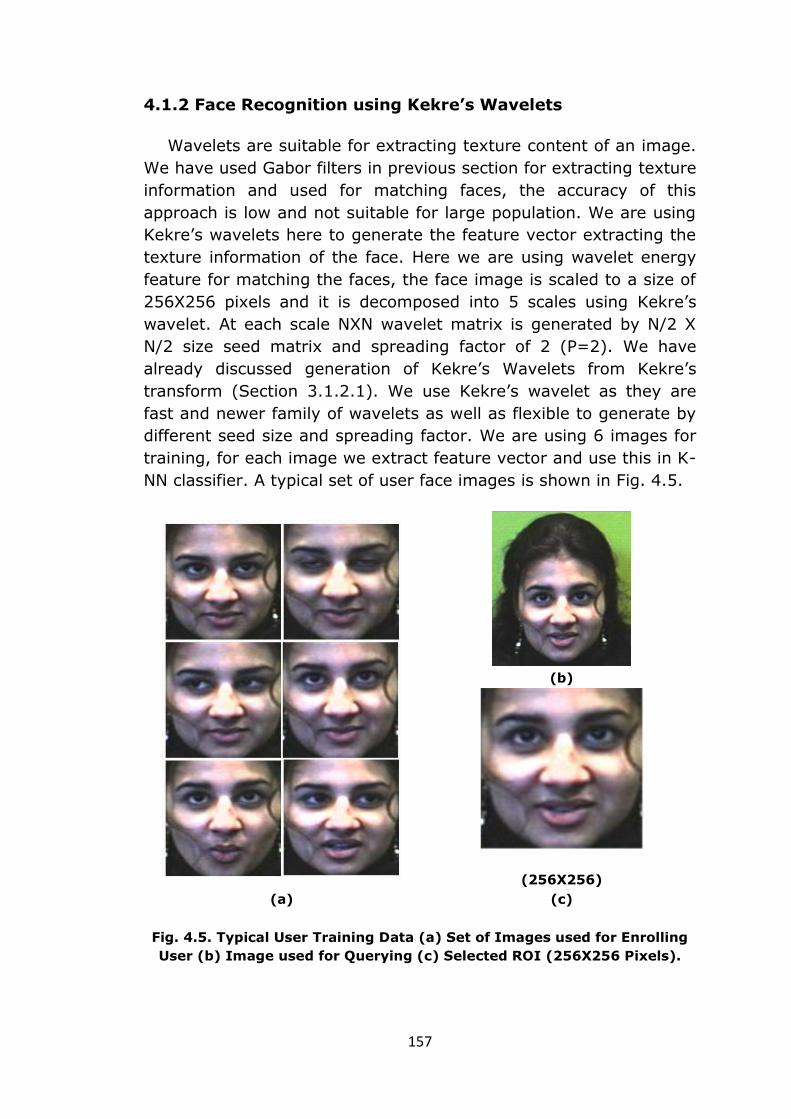
4.1.2 Face Recognition using Kekre’s Wavelets

Wavelets are suitable for extracting texture content of an image.

We have used Gabor filters in previous section for extracting texture

information and used for matching faces, the accuracy of this

approach is low and not suitable for large population. We are using

Kekre’s wavelets here to generate the feature vector extracting the

texture information of the face. Here we are using wavelet energy

feature for matching the faces, the face image is scaled to a size of

256X256 pixels and it is decomposed into 5 scales using Kekre’s

wavelet. At each scale NXN wavelet matrix is generated by N/2 X

N/2 size seed matrix and spreading factor of 2 (P=2). We have

already discussed generation of Kekre’s Wavelets from Kekre’s

transform (Section 3.1.2.1). We use Kekre’s wavelet as they are

fast and newer family of wavelets as well as flexible to generate by

different seed size and spreading factor. We are using 6 images for

training, for each image we extract feature vector and use this in K-

NN classifier. A typical set of user face images is shown in Fig. 4.5.

(b)

(256X256)

(a) (c)

Fig. 4.5. Typical User Training Data (a) Set of Images used for Enrolling

User (b) Image used for Querying (c) Selected ROI (256X256 Pixels).

158

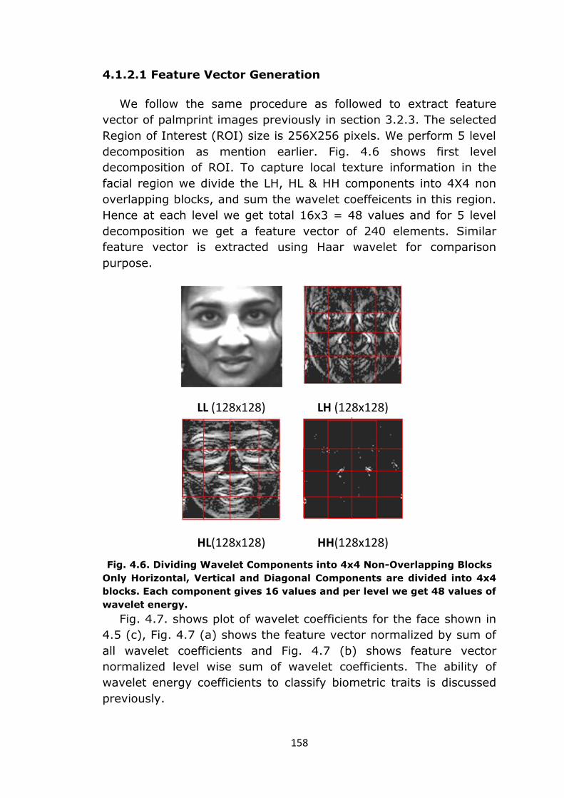
4.1.2.1 Feature Vector Generation

We follow the same procedure as followed to extract feature

vector of palmprint images previously in section 3.2.3. The selected

Region of Interest (ROI) size is 256X256 pixels. We perform 5 level

decomposition as mention earlier. Fig. 4.6 shows first level

decomposition of ROI. To capture local texture information in the

facial region we divide the LH, HL & HH components into 4X4 non

overlapping blocks, and sum the wavelet coeffeicents in this region.

Hence at each level we get total 16x3 = 48 values and for 5 level

decomposition we get a feature vector of 240 elements. Similar

feature vector is extracted using Haar wavelet for comparison

purpose.

LL (128x128) LH (128x128)

HL(128x128) HH(128x128)

Fig. 4.6. Dividing Wavelet Components into 4x4 Non-Overlapping Blocks

Only Horizontal, Vertical and Diagonal Components are divided into 4x4

blocks. Each component gives 16 values and per level we get 48 values of

wavelet energy.

Fig. 4.7. shows plot of wavelet coefficients for the face shown in

4.5 (c), Fig. 4.7 (a) shows the feature vector normalized by sum of

all wavelet coefficients and Fig. 4.7 (b) shows feature vector

normalized level wise sum of wavelet coefficients. The ability of

wavelet energy coefficients to classify biometric traits is discussed

previously.

159

(a)

(b)

Fig. 4.7. Kekre’s Wavelet Energy Feature Vector (a) Wavelet coefficients

normalized by total sum (b) Wavelet coefficients normalized level wise

We analyze this method for following modes for both Kekre’s

Wavelets & Haar Wavelets:

KFVN1 & KFVN2 – Kekre’s (Wavelet) Feature Vector

Normalized by total Energy (KFVN1) & Normalized by level

wise sum of Wavelet Energy (KFVN2), Euclidian Distance (ED)

between two KWEFV sequences (Seq. X & Seq. Y).

WEC & WEL – Wavelet Energy is calculated for each

component (WEC) and for each level (WEL). For WEC we get

16 X 3 = 48 coefficients & for WEL we get 5 components, we

evaluate Euclidian distance between these sequence.

RWEEC & RWEEL – Here we use the above mentioned WEC

and WEL sequence and convert them into probability

distributions by normalizing. We evaluate Relative Energy

Entropy between these sequences for matching faces. These

feature vectors are hence termed and Relative Wavelet

Energy Entropy Component wise (RWEEC) and Level wise

(RWEEL).

160

RKEEF –Relative Wavelet Energy Entropy for two normalized

Kekre’s Wavelet feature Vectors directly. We take full wavelet

energy coefficient sequence and normalize it by total energy.

This distribution is then used for finding full sequence relative

entropy. Hence it is termed as Relative Kekre’s (Wavelet)

Energy Entropy for Full Sequence (RKEEF).

Fig. 4.8. Relative Probability for Matching Distance of Genuine and

Forgery Tests for Kekre’s Wavelets based Feature Vectors. Two clear

classes can be seen, with threshold distance as 85. This can be used for

designing classifier.

4.1.2.2 Results

To justify the use of Kekre’s wavelet energy feature based

feature vector we have performed a comparison of Euclidian

distance between these feature vectors & that of Haar wavelets

feature vectors. This is shown in Fig. 4.9. This shows sorted

Euclidian distance (as per Kekere’s Wavelet FV) for performed tests

(Test 1 to Test 100) on X-axis and the corresponding distance on Y-

axis. First entry belongs to the matching face and further entries

belong to other faces. Fig. 4.9(a) shows the distance comparison

for all the features. The relative energy entropy based feature

vector performance is best; this is shown separately in Fig. 4.9(b)

along with that of Haar wavelets. We have also used weighted linear

fusion of all the distances and the final Euclidian distance plot is

shown in Fig. 4.9(c). All these graphs clearly show that the

matching user has lowest distance with test feature vector. Kekre’s

wavelet & Haar wavelets follow almost similar pattern.

0

5

10

15

20

25

30

40

60

80

10

0

12

0

14

0

16

0

18

0

20

0

22

0

24

0

26

0

28

0

30

0

32

0

34

0

36

0

38

0

40

0

42

0

44

0

46

0

48

0

50

0

Genuine Distance

Forgery Distance

% o

f O

ccu

ran

ce

Distance Range

161

(a)

(b)

(c)

Fig. 4.9. Normalized Distance for a Typical User (ID 24- First Entry) Face

Identification Vs User ID (a) Kekre’s Wavelet Based Features (b) Relative

Wavelet Energy Entropy Distance Shown Separately (c) Final Euclidian

Distance

0

0.5

1

1.5

2

2.5

3

3.5

4

1 6

11

16

21

26

31

36

41

46

51

56

61

66

71

76

81

86

91

96

No

rmal

ize

d D

ista

nce

Euclidian Distance for Kekre's Wavelet Based Feature Vector

KFVN1

KFVN2

WEC

WEL

RWEEC

RWEEL

RKEEF

Test Number

0

0.1

0.2

0.3

0.4

0.5

0.6

0.7

0.8

1 6

11

16

21

26

31

36

41

46

51

56

61

66

71

76

81

86

91

96

No

rmal

ize

d D

ista

nce

Relative Energy Entropy for Kekre's & Haar Wavelets Feature Vector

RKEEF

RHEEF

Test Number

0

5

10

15

20

25

30

35

1 6

11

16

21

26

31

36

41

46

51

56

61

66

71

76

81

86

91

96

No

rmal

ized

Dis

tan

ce

Final Euclidian Distance Plot for Kekre's & Haar Wavelets

ED

ED-Haar

Test Number

162

Next we perform FAR-FRR analysis for this method. In the database

we enrolled 100 users and for each user 6 images were taken for

training set. Total 410 tests are performed for intra-class matching

and 8112 tests are performed for inter class matching. K-NN

classifier based on the RWEE and Euclidian distance as discussed

earlier was used. We give results for Kekre’s wavelets based feature

vector first and then comparison is given.

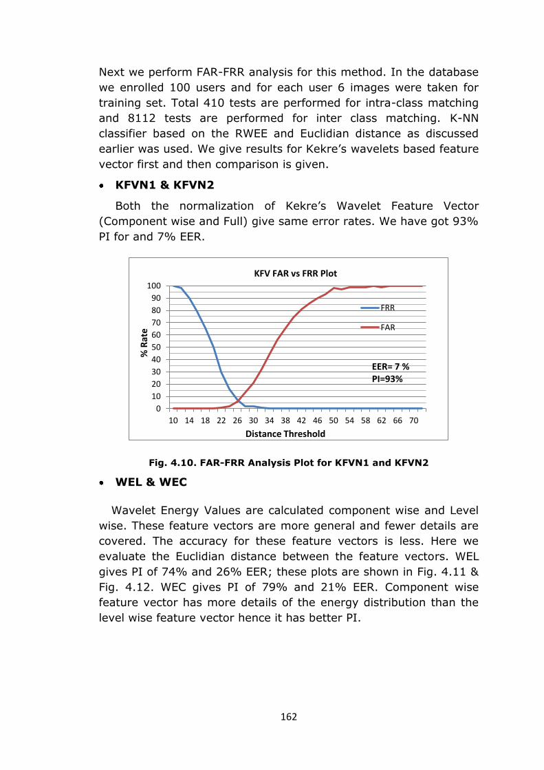
KFVN1 & KFVN2

Both the normalization of Kekre’s Wavelet Feature Vector

(Component wise and Full) give same error rates. We have got 93%

PI for and 7% EER.

Fig. 4.10. FAR-FRR Analysis Plot for KFVN1 and KFVN2

WEL & WEC

Wavelet Energy Values are calculated component wise and Level

wise. These feature vectors are more general and fewer details are

covered. The accuracy for these feature vectors is less. Here we

evaluate the Euclidian distance between the feature vectors. WEL

gives PI of 74% and 26% EER; these plots are shown in Fig. 4.11 &

Fig. 4.12. WEC gives PI of 79% and 21% EER. Component wise

feature vector has more details of the energy distribution than the

level wise feature vector hence it has better PI.

0

10

20

30

40

50

60

70

80

90

100

10 14 18 22 26 30 34 38 42 46 50 54 58 62 66 70

FRR

FAR

Distance Threshold

% R

ate

KFV FAR vs FRR Plot

EER= 7 % PI=93%

163

Fig. 4.11. Kekre’s Wavelet FAR-FRR Analysis Plot for Wavelet Entropy

Level wise (WEL)

Fig. 4.12. Kekre’s Wavelet FAR-FRR Analysis Plot for Wavelet Entropy

Component wise (WEC)

PI of WEC is better than that of WEL.

RWEEC & RWEEL

The above mentioned Wavelet Energy Sequences are used to

match the face by evaluating Relative Entropy here. We Evaluate

relative entropy both level & component wise. The relative entropy

gives better results in case of detailed wavelet energy distribution.

We have got PI of 93.5 & EER of 6.5 % respectively for relative

wavelet energy entropy component wise (RWEEC). This is shown in

0

10

20

30

40

50

60

70

80

90

100

0

10

20

30

40

50

60

70

80

90

10

0

11

0

12

0

13

0

14

0

15

0

16

0

FRR

FAR

EER = 26% PI=74%

WEL FAR vs FRR Plot

Distance Threshold

% R

ate

0

10

20

30

40

50

60

70

80

90

100

20

35

50

65

80

95

11

0

12

5

14

0

15

5

17

0

18

5

20

0

21

5

23

0

24

5

26

0

27

5

FRR

FAR

WEC FAR vs FRR Plot

% R

ate

Distance Threshold

EER = 21% PI=79%

164

Fig. 4.13. Fig 4.14 shows FAR-FRR plot of Relative Energy Entropy

Level wise (RWEEL), the EER is 24% & PI is 76% which is lower

than that of RWEEC.

Fig. 4.13. Kekre’s Wavelet FAR-FRR Analysis Plot for RWEEC

Fig. 4.14. Error Rate Analysis Plot for RWEEL FAR-FRR Plot

RKEEF

Relative Wavelet Energy Entropy for two normalized Kekre’s

Wavelet feature Vectors directly. We evaluate to normalized Kekre’s

Wavelet Energy sequences (240 Coefficients) and find the relative

entropy between two sequences for matching. This approach has

given best PI of 95% and that EER of 5%.

0102030405060708090

100

20

80

14

0

20

0

26

0

32

0

38

0

44

0

50

0

56

0

62

0

68

0

74

0

80

0

86

0

92

0

98

0

FRR

FAR

RWEEC FAR vs FRR Plot

Distance Threshold

% R

ate

EER= 6.5% PI=93.5%

0

10

20

30

40

50

60

70

80

90

100

12

0

12

4

12

8

13

2

13

6

14

0

14

4

14

8

15

2

15

6

16

0

16

4

16

8

17

2

FRR

FAR

RWEEL FAR vs FRR Plot

EER= 24 % PI=76%

Distance Threshold

% R

ate

165

Fig. 4.15. FAR-FRR Analysis Plot for RKEEF

We have performed fusion of KFVN2, RWEEC & RKEEF scores for

face recognition. The fused score analysis has given PI of 94% and

6% EER. In case of face recognition fusion has not given

performance improvements as in case of previous biometrics, face

images have lesser texture details as compared to fingerprint,

palmprint & finger-knuckle prints.

Fig. 4.16. FAR-FRR Analysis Plot for Fusion of Feature Vector

Table 4.2 lists all the Equal Error Rates (EER) & PI for different

feature vector combinations implemented for Kekre’s wavelets &

Haar wavelets. The comparison chart is shown in Fig. 4.17. We have

got maximum PI of 95% for Relative Kekre’s Energy Entropy Full

(RKEEF) feature vector, and the lowest PI is 74% for (Kekre’s)

0

10

20

30

40

50

60

70

80

90

100

0

15

30

45

60

75

90

10

5

12

0

13

5

15

0

16

5

18

0

19

5

21

0

FRR

FAR

RKEEF FAR vs FRR Plot

Distance Threshold

% R

ate

EER = 5% PI=95%

0

10

20

30

40

50

60

70

80

90

100

10

30

50

70

90

11

0

13

0

15

0

17

0

19

0

21

0

23

0

25

0

27

0

29

0

31

0

33

0

FRR

FAR

Distance Threshold

% R

ate

Fusion FAR vs FRR Plot

EER= 6 % PI=94%

166

Wavelet Energy Entropy Level wise (WEEL). The fusion gives

moderate performance with PI of 94%. This shows the superiority of

Relative Wavelet Energy Entropy based classifier.

Table 4.2

PI Comparison for Different Feature Vectors Derived for Kekre’s Wavelet

Energy Distribution

Sr. Feature

vector Type

Kekre’s Wavelets

PI

Haar Wavelets

PI

1 Fusion 94.00 90.50

2 KFVN2 93.00 90.20

3 RWEEL 76.00 74.00

4 RWEEC 93.50 88.50

5 WEEC 79.00 77.50

6 WEEL 74.00 73.50

7 RKEEF 95.00 91.40

Fig. 4.17. Comparison of EER for Kekre’s Wavelet Based Feature vector

Variants

Relative Kekre’s Energy Entropy of Full Sequence (RKEEF) Based Feature

Vector Gives Best Performance. This is Indicated by Red Bar

Kekre’s wavelets have given highest PI of 95 for Relative Energy

Entropy of full sequence of the wavelet energy (RKEEF). Fusion

gives next best performance. Haar wavelets give highest PI of 91.40

for Relative Energy Entropy of full sequence of the wavelet energy.

Kekre’s wavelets give higher PI as it can be seen from Fig. 4.17.

Fusion KFVN2 RWEEL RWEEC WEEC WEEL RKEEF

PI-Kekre 94 93 76 93.5 79 74 95

PI-Haar 90.5 90.2 74 88.5 77.5 73.5 91.4

0

10

20

30

40

50

60

70

80

90

100

% E

ER

Performance Comparison for Kekre's & Haar Wavelet based Feature Vector for Face Recognition

167

Total 410 tests are performed for intra-class matching and 8112

tests are performed for inter class matching. K-NN classifier based

on the RWEE and Euclidian distance as discussed earlier was used.

This testing is carried for both Kekre’s & Haar wavelets, the analysis

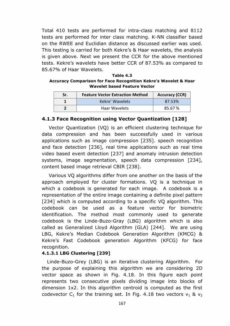
is given above. Next we present the CCR for the above mentioned

tests. Kekre’s wavelets have better CCR of 87.53% as compared to

85.67% of Haar Wavelets.

Table 4.3

Accuracy Comparison for Face Recognition Kekre’s Wavelet & Haar

Wavelet based Feature Vector

Sr. Feature Vector Extraction Method Accuracy (CCR)

1 Kekre’ Wavelets 87.53%

2 Haar Wavelets 85.67 %

4.1.3 Face Recognition using Vector Quantization [128]

Vector Quantization (VQ) is an efficient clustering technique for

data compression and has been successfully used in various

applications such as image compression [235]. speech recognition

and face detection [236], real time applications such as real time

video based event detection [237] and anomaly intrusion detection

systems, image segmentation, speech data compression [234],

content based image retrieval CBIR [238].

Various VQ algorithms differ from one another on the basis of the

approach employed for cluster formations. VQ is a technique in

which a codebook is generated for each image. A codebook is a

representation of the entire image containing a definite pixel pattern

[234] which is computed according to a specific VQ algorithm. This

codebook can be used as a feature vector for biometric

identification. The method most commonly used to generate

codebook is the Linde-Buzo-Gray (LBG) algorithm which is also

called as Generalized Lloyd Algorithm (GLA) [244]. We are using

LBG, Kekre’s Median Codebook Generation Algorithm (KMCG) &

Kekre’s Fast Codebook generation Algorithm (KFCG) for face

recognition.

4.1.3.1 LBG Clustering [239]

Linde-Buzo-Grey (LBG) is an iterative clustering Algorithm. For

the purpose of explaining this algorithm we are considering 2D

vector space as shown in Fig. 4.18. In this figure each point

represents two consecutive pixels dividing image into blocks of

dimension 1x2. In this algorithm centroid is computed as the first

codevector C1 for the training set. In Fig. 4.18 two vectors v1 & v2

168

are generated by adding constant error to the codevector. Euclidean

distances of all the training vectors are computed with vectors v1 &

v2 and two clusters are formed based on nearest of v1 or v2.

Procedure is repeated for these two clusters to generate four new

clusters. This procedure is repeated for every new cluster until the

required size of codebook is reached or specified MSE is reached.

The drawback of this algorithm is that the cluster elongation is

+135o to horizontal axis in two dimensional case. This results in

inefficient clustering.

Fig. 4.18. LBG for 2 Dimensional Case

The database images are divided into the block of 2x2 pixels from

each block are arranged in a single row. Then the mean of the each

column is calculated. This mean value is a coordinate for the first

codevector C1. After that a constant error of +1 and -1 is added to

the C1 to get two more code vectors. The existing blocks are now

compared with the newly generated code vectors C1’ and C1’’

respectively and for each of them the Euclidian distance is

calculated. Whichever code vector gives minimum Euclidian distance

the blocks are place in that particular cluster. So after first iteration

two different and non-overlapping clusters are formed. For these

clusters now the procedure is repeated to get clusters in multiple of

two and code book is prepared.

4.1.3.2 Kekre’s Median Codebook Generation Algorithm

In [240] the Kekre & Sarode have proposed this algorithm for

image data compression. This algorithm reduces the time for code

book generation. It uses sorting and median technique for codebook

generation.

169

kMMM

k

k

xxx

xxx

xxx

T

,2,1,

,22,21,2

,12,11,1

....

.

.

.

.

.

.

.

.

....

....

(4.5)

In this algorithm image is divided into blocks and blocks are

converted to the vectors of size k. The Eqn. 4.5 given below

represents matrix T of size M x k consisting of M number of image

training vectors of dimension k. Each row of the matrix is the image

training vector of dimension k. The training vectors are sorted with

respect to the first component of all the vectors i.e. with respect to

the first column of the matrix T and the entire matrix is considered

as one single cluster. The median of the matrix T is chosen

(codevector) and is put into the codebook, and the size of the

codebook is set to one. The matrix is then divided into two equal

parts and each of the part is then again sorted with respect to the

second component of all the training vectors i.e. with respect to the

second column of the matrix T and we obtain two clusters both

consisting of equal number of training vectors. The median of both

the parts is picked up and written to the codebook, now the size of

the codebook is increased to two, consisting of two codevectors and

again each part is further divided to half. Each of the above four

parts obtained are sorted with respect to the third column of the

matrix T and four clusters are obtained and accordingly four

codevectors are obtained. The above process is repeated till we

obtain the codebook of desired size. Here quick sort algorithm is

used. This algorithm takes least time to generate codebook, since

Euclidean distance computation is not required.

Vector Quantization is basically the clustering algorithm, where

the image is divided into pixel windows. These pixel windows give

the texture information of the image. Smaller the window size finer

texture details will be represented. Bigger pixel window gives coarse

texture details of image. The better option is to select medium size

of window as 2x2 or 3x3. Here we have divided images in 2x2 pixel

windows because we have used color images. The window is then

converted into vector of size 12 to form training vector set, since for

170

3x3 window size the vector dimension will be 27 increasing

computational complexity in that ratio. The Kekre’s Median

Codebook Generation (KMCG) algorithm is applied on this set to get

feature vector of size 128*12 for the face image.

4.1.3.3 KMCG Based Feature Vector Generation

Kekre & Shah have performed study of VQ Codebook size and its

effect on face recognition [126]. Different codebook of size of 32,

64, 128 & 256 has been studied. It is found that codebook size of

256 gives best performance for local database used but it has

marginal improvement over codebook of size 128 and their

performance was equal for the ORL face database used. To reduce

the size of feature vector we select codebook of size 128 elements.

Here the feature vector space has 128*12 numbers of elements.

This is obtained using following steps of Kekre’s Median Codebook

Generation (KMCG) algorithm

1. Image is divided into the windows of size 2x2 pixels (each

pixel consisting of red, green and blue components).

2. These are put in a row to get 12 values per vector. Collection

of these vectors is a training set.

3. The training set is sorted with respect to first column. The

centre value of first column is used to divide the training set

in two parts.

4. Further each part is then separately sorted with respect to

second column to get two centre values.

5. The process of sorting is repeated till we get 128 centre

values.

6. Using these centre values as codevectors, Codebook of size

128*12 is generated

7. The codebook is stored as the feature vector for the image.

Thus the feature vector database is generated.

8. Query Execution- Here the codebook of size 128*12 for the

query image is extracted using Kekre’s Median Codebook

Generation Algorithm and the feature vector of query image is

obtained. Then this feature set is compared with other feature

sets in feature database using Euclidian distance as similarity

measure.

4.1.3.4 Kekre’s Fast Codebook Generation Algorithm (KFCG)

Here the Kekre’s Fast Codebook Generation algorithm proposed

in [234] for image data compression is used. This algorithm reduces

the time for code book generation. Initially we have one cluster with

171

the entire training vectors and the codevector C1 which is centroid.

In the first iteration of the algorithm, the clusters are formed by

comparing first element of training vector with first element of code

vector C1.

(a) First Iteration

(b) Second Iteration

Fig. 4.19. KFCG for 2 Dimensional Case

The vector Xi is grouped into the cluster 1 if xi1< c11 otherwise

vector Xi is grouped into cluster 2 as shown in Fig. 4.19(a), Where

codevector dimension space is 2. In second iteration, the cluster 1

is split into two by comparing second element xi2 of vector Xi

belonging to cluster 1 with that of the second element of the

codevector. Cluster 2 is split into two by comparing the second

element xi2 of vector Xi belonging to cluster 2 with that of the

second element of the codevector as shown in Fig. 4.19(b). This

procedure is repeated till the codebook size is reached to the size

specified by user. It is observed that this algorithm gives less error

172

as compared to LBG and requires least time to generate codebook

as compared to KMCG, as it does not require any computation of

Euclidean distance. Codebook generation procedure is same as

discussed in case of KMCG in previous section (Section 4.1.3.3).

4.1.3.5 Results

We have discussed LBG, KFCG and KMCG based feature vectors

for face recognition. These algorithms are now applied to the

compressed form of the database image and then to the query

image and the apparent match are sent as the result. We are using

Georgia Tech Database for this [243]. It consists of 750 images of

50 persons; each person has 15 face images as shown in Fig. 4.20.

Out of these images 9 images are used for training and six images

are used for testing. Each of these algorithms were implemented in

MATLAB 7.0 on Intel Pentium Dual Core Processor (2.01 GHz), 2GB

RAM on Windows XP Professional SP3.

(a)

(b)

Fig. 4.20. Database Images (a) and (b) represents 15 Images of 2

Subjects in the Database

Accuracy shown here implies the number of correctly identified

faces to the total number of images queried for recognition. This is

summarized in Table 4.4 & Fig. 4.21.

173

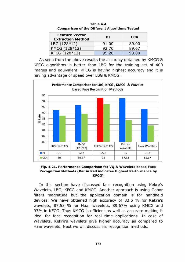
Table 4.4

Comparison of the Different Algorithms Tested

Feature Vector

Extraction Method PI CCR

LBG (128*12) 91.00 89.00

KMCG (128*12) 92.70 89.67

KFCG (128*12) 95.20 93.00

As seen from the above results the accuracy obtained by KMCG &

KFCG algorithms is better than LBG for the training set of 400

images and equivalent. KFCG is having highest accuracy and it is

having advantage of speed over LBG & KMCG.

Fig. 4.21. Performance Comparison for VQ & Wavelets based Face

Recognition Methods (Bar in Red indicates Highest Performance by

KFCG)

In this section have discussed face recognition using Kekre’s

Wavelets, LBG, KFCG and KMCG. Another approach is using Gabor

filters magnitude but the application domain is for handheld

devices. We have obtained high accuracy of 83.5 % for Kekre’s

wavelets, 87.53 % for Haar wavelets, 89.67% using KMCG and

93% in KFCG. Thus KMCG is efficient as well as accurate making it

ideal for face recognition for real time applications. In case of

Wavelets, Kekre’s wavelets give higher accuracy as compared to

Haar wavelets. Next we will discuss iris recognition methods.

LBG (128*12)KMCG

(128*12)KFCG (128*12)

KekresWavelets

Haar Wavelets

PI 91 92.7 95.2 95 91.4

CCR 89 89.67 93 87.53 85.67

80

82

84

86

88

90

92

94

96

% R

ate

Performance Comparison for LBG, KFCG , KMCG & Wavelet based Face Recognition Methods

174

4.2 Iris Recognition

Iris recognition enjoys universality, high degree of uniqueness

and moderate user cooperation. This makes Iris recognition systems

unavoidable in emerging security & authentication mechanisms. In

today’s world, where terrorist attacks are on the rise, employment

of infallible security systems is a must. The identification of a person

or an individual on the basis of their biometric characteristics like

fingerprint, face, speech, and iris is thus gaining importance. Iris

recognition is one of the important techniques and it is rotation and

aging invariant. Compared with other biometric features (such as

face, voice, etc.), the iris is more stable and reliable for

identification [131].

Iris is the central part of the eye surrounding the pupil. Iris

Recognition is the analysis of the colored ring that surrounds the

pupil [1]. The iris has unique structure and these patterns are

randomly distributed; which can be used for identification of human

being. Typical iris is shown in the eye image in the Fig. 4.22. With

fast development of iris image acquisition technology, iris

recognition is expected to become a fundamental component of

modern society, with wide application areas in national ID card,

banking, e-commerce, welfare distribution, biometric passport, and

forensics, etc. Since 1990s, research on iris image processing and

analysis has achieved great progress [1].

Fig. 4.22. Eye Image Showing Iris, Pupil & Sclera

Generally, iris recognition system consists of four major steps.

They include image acquisition from iris scanner, iris image

preprocessing, feature extraction and enrollment & recognition.

Image acquisition is a very important process as iris image with bad

175

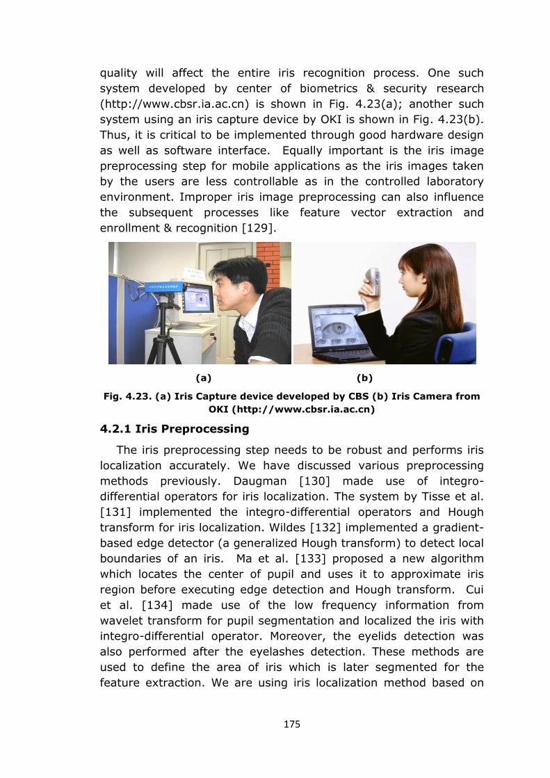
quality will affect the entire iris recognition process. One such

system developed by center of biometrics & security research

(http://www.cbsr.ia.ac.cn) is shown in Fig. 4.23(a); another such

system using an iris capture device by OKI is shown in Fig. 4.23(b).

Thus, it is critical to be implemented through good hardware design

as well as software interface. Equally important is the iris image

preprocessing step for mobile applications as the iris images taken

by the users are less controllable as in the controlled laboratory

environment. Improper iris image preprocessing can also influence

the subsequent processes like feature vector extraction and

enrollment & recognition [129].

(a) (b)

Fig. 4.23. (a) Iris Capture device developed by CBS (b) Iris Camera from

OKI (http://www.cbsr.ia.ac.cn)

4.2.1 Iris Preprocessing

The iris preprocessing step needs to be robust and performs iris

localization accurately. We have discussed various preprocessing

methods previously. Daugman [130] made use of integro-

differential operators for iris localization. The system by Tisse et al.

[131] implemented the integro-differential operators and Hough

transform for iris localization. Wildes [132] implemented a gradient-

based edge detector (a generalized Hough transform) to detect local

boundaries of an iris. Ma et al. [133] proposed a new algorithm

which locates the center of pupil and uses it to approximate iris

region before executing edge detection and Hough transform. Cui

et al. [134] made use of the low frequency information from

wavelet transform for pupil segmentation and localized the iris with

integro-differential operator. Moreover, the eyelids detection was

also performed after the eyelashes detection. These methods are

used to define the area of iris which is later segmented for the

feature extraction. We are using iris localization method based on

176

Circular Hough Transform. Iris Recognition is studied with and

without localization.

The iris localization is a two-step process,

1. Find the canny edges of the iris image.

2. Apply Circular Hough Transform [133] to the canny edge

image with iris parameters.

3. Locate the iris center by quantization of Hough Magnitude.

4.2.1.1 Canny Edge Detection of Iris Image

The purpose of edge detection in general is to significantly

reduce the amount of data in an image, while preserving the

structural properties to be used for further image processing. Canny

edge detection is optimal with regards to the following criteria [46]:

1. Detection: The probability of detecting real edge points

should be maximized while the probability of falsely

detecting non-edge points should be minimized. This

corresponds to maximizing the signal-to-noise ratio.

2. Localization: The detected edges should be as close as

possible to the real edges.

3. Number of responses: One real edge should not result in

more than one detected edge (one can argue that this is

implicitly included in the first requirement).

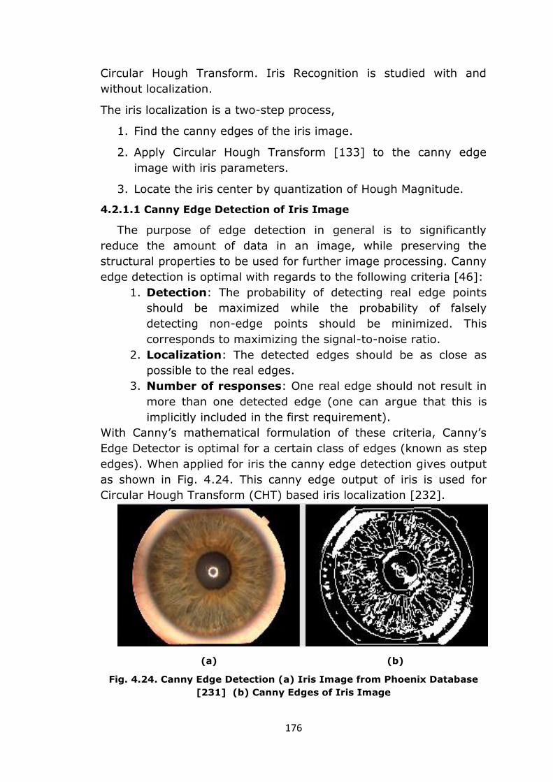
With Canny’s mathematical formulation of these criteria, Canny’s

Edge Detector is optimal for a certain class of edges (known as step

edges). When applied for iris the canny edge detection gives output

as shown in Fig. 4.24. This canny edge output of iris is used for

Circular Hough Transform (CHT) based iris localization [232].

(a) (b)

Fig. 4.24. Canny Edge Detection (a) Iris Image from Phoenix Database

[231] (b) Canny Edges of Iris Image

177

4.2.1.2 Iris Localization using Circular Hough Transform [232]

Hough transform is a technique which can be used to isolate

features of a particular shape within an image. Because it requires

the desired features to be specified in some parametric form, the

classical Hough transform is most commonly used for the detection

of regular curves such as lines, circles, ellipses etc. [46]. The main

advantage of the Hough transform technique is that it is tolerant to

gaps in feature boundary descriptions and is relatively unaffected by

image noise. To detect the eye which is circular in shape the so

called Circular Hough Transform is used as in equation,

2 2 2

0 0( ) ( )x x y y r (4.6)

Where, (x0,y0) is the coordinate of the circle center, r is the

radius of the circle. The detection process starts with the local

maxima in the group of the area of interest is assumed as the

center of the circle.

(a)

(b)

Fig. 4.25. Iris Localization (a) Hough Magnitude Plot for the Iris Edge

Map Shown in Fig. 4.24 (b). (b) Localized Iris

The Hough magnitude is calculated for predefined radius of

search. The phoenix database of iris is having iris radius in the

range 220 to 260 pixels. The Hough magnitude is calculated for

radius if 240 pixels (Average Value). If the linear indices among the

minimum value of qualified pixel forming the circular shape, then

that area is the iris region detected on the image. Every area of

178

interest is tested with this process for it occurs as an element of the

circle component which is the iris region identified in the image.

This is done by thresholding of the Hough magnitude and

selecting point satisfying the criteria of radius. Fig. 4.25 shows iris

Hough magnitude map. The red region shows Hough Space points

[232] satisfying the centroid criteria of circle with radius of 240

pixels. This map is then thresholded and the centroid of iris is

localized. The iris localization process is shown in Fig. 4.25, this

shows the localized iris circle on canny edge map as well as on the

iris image. The localized iris parameters are used to unwrap the iris

this is called as iris normalization.

First we will discuss methods without iris localization and then we

compare results with iris localization.

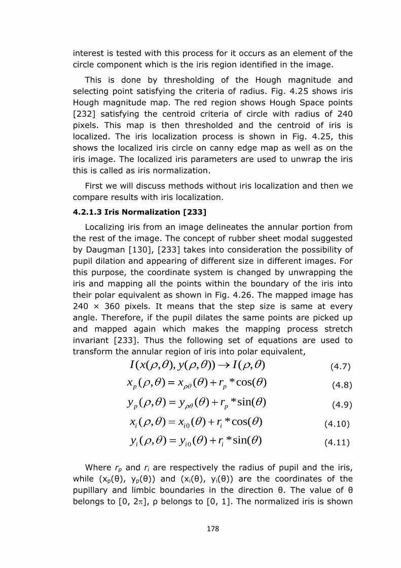
4.2.1.3 Iris Normalization [233]

Localizing iris from an image delineates the annular portion from

the rest of the image. The concept of rubber sheet modal suggested

by Daugman [130], [233] takes into consideration the possibility of

pupil dilation and appearing of different size in different images. For

this purpose, the coordinate system is changed by unwrapping the

iris and mapping all the points within the boundary of the iris into

their polar equivalent as shown in Fig. 4.26. The mapped image has

240 × 360 pixels. It means that the step size is same at every

angle. Therefore, if the pupil dilates the same points are picked up

and mapped again which makes the mapping process stretch

invariant [233]. Thus the following set of equations are used to

transform the annular region of iris into polar equivalent,

( ( , ), ( , )) ( , )I x y I (4.7)

( , ) ( ) *cos( )p px x r (4.8)

( , ) ( ) *sin( )p py y r (4.9)

0( , ) ( ) *cos( )i i ix x r (4.10)

0( , ) ( ) *sin( )i i iy y r (4.11)

Where rp and ri are respectively the radius of pupil and the iris,

while (xp(θ), yp(θ)) and (xi(θ), yi(θ)) are the coordinates of the

pupillary and limbic boundaries in the direction θ. The value of θ

belongs to [0, 2 ], ρ belongs to [0, 1]. The normalized iris is shown

179

in Fig. 4.26 (c). This is iris Region of Interested (ROI) segmented or

Normalized Iris, this ROI can be used for feature extraction.

(a) (b) (c)

Fig. 4.26. Unwrapping Iris (a) Input Iris Image (b) Localized Iris (c)

Unwrapped (Normalized) Iris.

Iris normalization gives better quality of input for the feature

extraction process, this helps to improve the recognition rate. Iris

recognition with and without normalization will be discussed in the

next sections.

4.2.2. Iris Recognition using Vector Quantization [234]

We have discussed Vector Quantization techniques in previous

section on face recognition. LBG clustering is conventional algorithm

for vector quantization, while KFCG, KMCG are newer algorithms

and they are quite popular. Here we apply KMCG & KFCG for iris

feature vector extraction & matching, their performance is

compared with the LBG clustering algorithm.

4.2.2.1 Proposed VQ based Iris Recognition Method

We have selected codebook of size 128. Thus the feature vector

space has 128 x12 numbers of elements. Following are the steps to

obtain the Feature vector database.

1. Image is divided into the windows of size 2x2 pixels (each pixel

consisting of red, green and blue components).

2. These are put in a row to get 12 values per vector. Collection

of these vectors is a training set (initial cluster).

3. Compute centroid (codevector) of the cluster.

4. Apply LBG/KMCG/KFCG algorithm to obtained codebook of size

128.The codebook obtained is stored as the feature vector for

the image.

5. Query Execution- Here the codebook of size 128x12 for the

query image is extracted using LBG/ KMCG /KFCG and the

feature vector of query image is obtained. This feature set is

compared with other feature sets in feature database using

Euclidian distance.

180

4.2.2.2 Results for VQ based Methods

In any of the above implemented algorithms, we have not done

any preprocessing on the iris images in the database or the query

images. Also the images don’t solely contain the iris but also the

sclera surrounding it. We have used phoenix database [246]

consisting of irises of 64 individuals. Each individual has 3 images

corresponding to the left and 3 images corresponding to the right

eye. Six iris images in Portable Network Graphics (PNG) format of

each individual were taken into consideration. Thus in all there were

(64 X 6) 384 such images as a part of our database. We have

resized each image to a 128 x 128 color pixels. Thus, we have a 3-

dimensional array data for sized 128 x 128 x 3.

We have discussed LBG, KMCG & KFCG based feature vectors

earlier. These algorithms are now applied to the database image

and then to the query image and the apparent match are sent as

the result. Each of these algorithms were implemented in MATLAB

7.0 on Intel Pentium Dual Core Processor (2.01 GHz), 2GB RAM on

Windows XP Professional SP3.

For testing purpose we have retained two images each of left and

right eye in the database and one image each is used as query

image. Here we have tested the method by giving left/right query

images which is checked for the entire database of left as well as

right iris images. In few cases it has happened that the left query

image has given best match with the right iris image of the same

person, this is also treated as success.

The accuracy (CCR) is calculated as,

1Accuracy for Left Eye 100L

N

N (4.13)

2Accuracy for Right Eye 100R

N

N (4.14)

Where,

N1= No. of correct individual identified for Left iris query images.

NL= Total no. of Left iris images queried (64).

N2= No. of correct individuals identified for Right iris images.

NR= Total no. of Right iris images queried (64).

N= Total Number of Images in the database (NL+NR) (128)

1 2( )Overall Accuracy 100

N N

N (4.15)

181

Table 4.5

Comparison of the Different VQ Algorithms Tested for Iris Recognition

VQ

Algorithm

PI CCR Total Performance

PI-L PI-R CCR-L CCR-R PI-L+R CCR-L+R

LBG 79.50 87.50 78.13 84.38 83.60 81.25

KMCG 85.20 87.50 83.50 85.30 89.20 87.10

KFCG 89.90 92.00 87.50 90.63 91.40 89.10

Fig. 4.27. Performance Comparison between LBG, KMCG & KFCG

Graph Shows PI, CCR for Left, Right and combined Iris Testing. Combined

(L+R) Iris Recognition Gives Higher Performance. Performance of KFCG

is Highest.

Here we have discussed Iris Recognition using Vector

Quantization based on LBG, KMCG & KFCG Algorithms. We have

implemented these algorithms on iris image without any pre-

processing or segmentation including iris localization in spite of

which it has been possible for us to obtain such a high accuracy.

Table 4.5 & Fig. 4.27 show the comparison of the results. This is an

example of multi-instance biometrics. We have tested left & right

irises separately as well as combined testing is also done. KFCG

has the best performance with the accuracy of 89.10% as compared

to LBG and KPE. LBG has lowest PI & EER. If we combine these

methods with iris pre-processing the results can still be improved.

This is discussed next.

70

75

80

85

90

95

LBG KMCG KFCG

% R

ate

Vector Quantization Technique used for Feature Vector Generation

Performance Comparison for LBG, KMCG & KMCG for Iris Recognition

PI-L

PI-R

CCR-L

CCR-R

PI-L+R

CCR-L+R

182

4.2.3 Iris Recognition using Walsh & DCT

In this section we discuss a novel iris recognition method which

reduces the computational complexity and increases the accuracy.

We have tested full 2-dimensional Discrete Cosine Transform (DCT),

full 2-dimensional Walsh Transform (also known as Walsh

Hadamard Transform (WHT)), and the proposed method DCT/WHT

row mean and column mean.

4.2.3.1 Walsh Transform & DCT Based Feature Extraction

The DCT/WHT algorithm that we have used for our study on iris

recognition is as shown below:

1. Read the database image (Size=128X128).

2. Extract the Red, Green and Blue component of that image

such that each is of size 128X128.

3. Apply DCT/WHT to each component and append in a new row

the result for each Red, Green and Blue in matrix form. So we

get 128X384 entries. This is the Feature Vector (F.V) of that

image.

4. Repeat steps 1 through 3 for every database image.

5. Read the Query image.

6. Repeat step 2 and 3 for the query image so as to obtain its

Feature Vector.

7. For every Database image ‘i’ and a Query image ‘q’ Calculate

the Mean Squared Error using the following formula:

2

1. . [ ( ) ( )]

0

MS E FV i FV q

m (4.16)

[ ] (128*128*3)MSE i SE (4.17)

8. Determine the minimum M.S.E and corresponding image

matching iris.

We discuss the accuracy of this method in the results section, next

we discuss the Proposed DCT/WHT row mean, and column mean

based iris recognition method.

4.2.3.2 Row Mean & Column Mean of DCT& WHT Coefficients

Here we extend the study further by addition of one more

feature based on Row & Column Mean of iris image data. This

approach captures iris texture information by taking row wise &

column wise mean. This is process is shown in Fig. 4.31. We take

mean of grey levels of all pixels in ith Row to calculate Row Mean

(RMi) of ith row.

183

This gives Row Mean vector,

RM = {RM1, RM2, ……., RMm} (m= No. of Rows) (4.18)

Similarly for columns we get the Column Mean Vector CM given by,

CM = {CM1, CM2, ……., CMn} (n= No. of Columns) (4.19)

RM & CM are one dimensional (1D) vectors. We apply the one

dimensional (1D) DCT & WHT on the vectors to generate 1D DCT

Row Mean (RM) & Column Mean (CM) feature vector.

Fig. 4.28. Generation of Row Mean (RM) & Column Mean (CM) vector

From Iris Image Grey Level Values Cij

4.2.3.3 Proposed Iris Recognition Method

1. Read the database image (Size=128x128x3). Extract the Red,

Green and Blue component of that image such that each is of

size 128x128.

2. To prepare column mean vector. Here we take average of all

intensity values of pixels in each column of iris image and

construct a vector of all column means as discussed in

previous section.

3. To prepare row mean vector. Here we take average of all

intensity values of pixels in each row of iris image and

construct a vector of all row means.

4. DCT / WHT Features of column mean vector. Apply DCT/WHT

on the column mean vector of iris image and store the DCT/

WHT coefficients as feature vector part one.

5. DCT / WHT Features of row mean vector. Apply DCT / WHT on

the row mean vector of iris image and store the DCT / WHT

coefficients as feature vector part two.

6. Matching of DCT / WHT features The DCT / WHT features of

184

part one and two are matched with all entries in the database

DCT features part one and two respectively. Using squared

Euclidian distance the best match is found.

4.2.3.4 Results for DCT/WHT Based Iris Recognition

In any of the above implemented algorithms, we have not done

any preprocessing on the iris images in the database or the query

images. Also the images don’t solely contain the iris but also the

sclera surrounding it. We have used phoenix database [252]

consisting of irises of 64 individuals. Each individual has 3 images

corresponding to the left and 3 images corresponding to the right

eye. Six iris images in Portable Network Graphics (PNG) format of

each individual were taken into consideration. Thus in all there were

(64 X 6) 384 such images as a part of our database. We have

resized each image to a 128 x 128 color pixels. Thus, we have a 3-

dimensional image sized 128 x 128 x 3.

Table 4.6

Results for DCT/WHT RM & CM based Iris Recognition

(a) Results for DCT Row Mean and Column Mean

Algorithm PI CCR Total Performance


DCT 57.10 74.60 55.38 72.14 66.50 64.21

DCT-RM 68.60 81.70 64.25 79.55 77.10 74.96

DCT-CM 62.40 75.40 59.22 74.11 69.90 68.55

(b) Results for WHT Row Mean and Column Mean

Algorithm PI CCR Total Performance


WHT 62.00 75.20 59.38 73.44 68.70 66.10

WHT-RM 69.30 85.20 67.18 84.37 78.70 75.78

WHT-CM 81.20 82.90 65.62 79.68 74.60 72.65

We have discussed full 2-D DCT & WHT and Row mean, Column

mean DCT & WHT based feature vectors earlier. These methods are

now applied to the Phoenix database image and then to the query

image and the apparent match are sent as the result. Each of these

algorithms were implemented in MATLAB 7.0 on Intel Pentium Dual

Core Processor (2.01 GHz), 2GB RAM on Windows XP Professional

SP3. For testing purpose we have retained two images each of left

and right eye in the database and one image each is used as query

image. Table 4.6 gives the summary of performance of individual

method tested. Finally we summarize the performance of all the iris

185

recognition systems discussed up till now and results are presented

in Fig. 4.29.

Fig. 4.29. Performance Comparison for Iris Recognition Methods based

on DCT/WHT Row Mean & Column Mean

In this section we have discussed iris recognition using full 2-D

DCT, full 2-D Walsh transform, DCT on row/column mean and Walsh

transform on row/column mean. We have implemented these

algorithms on iris image without any pre-processing or

segmentation including iris localization in spite of which it has been

possible for us to obtain such a high accuracy. Row mean DCT/WHT

gives the best performance with the accuracy of 74.96% for DCT &

75.78% for WHT. Full DCT & WHT has low accuracy around 64.21 %

for DCT & 66.10% for WHT. Another thing is that the combined

Left+ Right iris is coming low because of large difference between

CCR of left & right iris testing. This is shown in Table 4.6 (a) & (b).

All the testing results indicate that the WHT has given better

performance than DCT.

DCT DCT-RM DCT-CM WHT WHT-RM WHT-CM

PI-L+R 66.5 77.1 69.9 68.7 78.7 74.6

CCR-L+R 64.21 74.96 68.55 66.1 75.78 72.65

0

10

20

30

40

50

60

70

80

90%

Rat

e

Performance Comparison of DCT & WHT based Iris Recognition Techniques

186

4.3 Iris Recognition with Preprocessing

In the previous sections iris recognition techniques based on

Walsh & DCT as well as vector quantization algorithms have been

discussed. These techniques were using iris images without

preprocessing. The full iris image was considered for feature

extraction, as the main par the iris texture pattern, the other part of

the image besides texture pattern is useless. The iris normalization

process helps to separate and unwrap the circular iris texture

pattern. The effect of iris normalization is studied in this section.

4.3.1 VQ Based Feature Extraction

In the section 4.2.3.2 the Walsh transform and DCT is used for

iris feature extraction, the unwrapped iris is used for feature

extraction process. The dimension of unwrapped iris ROI is 240*

360 pixels. After further removal of central dark part from the

(pupil) the final ROI Dimensions are 180*360 Pixels, as shown in

Fig. 4.26(c). This ROI is used for VQ based feature extraction. Here

LBG, KMCG & KFCG clustering algorithms are used to generate the

codebook feature vector. The testing is performed with the same

test parameters as discussed previously. The test results are

summarized in Table 4.7 & Fig. 4.30. Testing is performed on left,

Right & Combined (Left + Right) iris. This is an example of multi-

instance iris recognition. The iris recognition for Left + Right testing

is shown in column of Total Performance. Total performance is

higher that individual left & right iris recognition performance.

Amongst the different VQ methods KFCG gives best performance by

giving PI of 96.12%, EER of 3.88% & CCR of 95.18%. Next we

discuss DCT/WHT based iris Recognition.

Table 4.7

Comparison of the Different VQ Algorithms Tested for Iris Recognition

with Preprocessing

VQ

Algorithm

PI CCR Total Performance


LBG 87.50 81.90 86.21 80.36 86.90 86.70

KMCG 90.10 90.50 88.13 87.82 93.20 92.12

KFCG 92.00 92.70 91.21 90.01 96.10 95.18

187

Fig. 4.30. Performance Comparison LBG, KMCG, KFCG based Feature

Vectors for Iris Recognition Methods

Graph Shows PI, CCR for Left, Right and combined Iris Testing. Combined

(L+R) Iris Recognition Gives Higher Performance. Performance of KFCG

is Highest.

4.3.2 Walsh Transform & DCT Based Feature Extraction

After proper scaling normalized iris ROI is used for row and

column mean based feature extraction process discussed

previously. The testing is performed on phoenix database used

previously with same test parameters. Iris images for Left and Right

eye are enrolled separately and individual as well as fusion based

testing is performed. When both Left and Right iris images are used

for testing of a single user, it is called as a multi-instance biometric

system [21]. As compared to results given for DCT/WHT based

feature vectors in Table 4.6, the results in Table 4.8 are higher. DCT

Row mean has given higher performance index 90.89% and CCR of

89.21% in DCT based feature vector group. In case of WHT based

group column mean feature vector gives higher performance, it

gives 95.48% PI & 93% CCR. In both the cases of iris recognition

with and without preprocessing, WHT has outperformed DCT based

methods.

Next we discuss the performance improvement achieved due to

preprocessing & normalization of Iris ROI. Fig. 4.31 & Table 4.9

summarize these results.

50

60

70

80

90

100

LBG KMCG KFCG

% R

ate

Vector Quantization Technique used for Feature Vector Generation

Performance Comparison for LBG, KMCG & KMCG for Iris Recognition with Preprocessing

PI-L

PI-R

CCR-L

CCR-R

PI-L+R

CCR-L+R

188

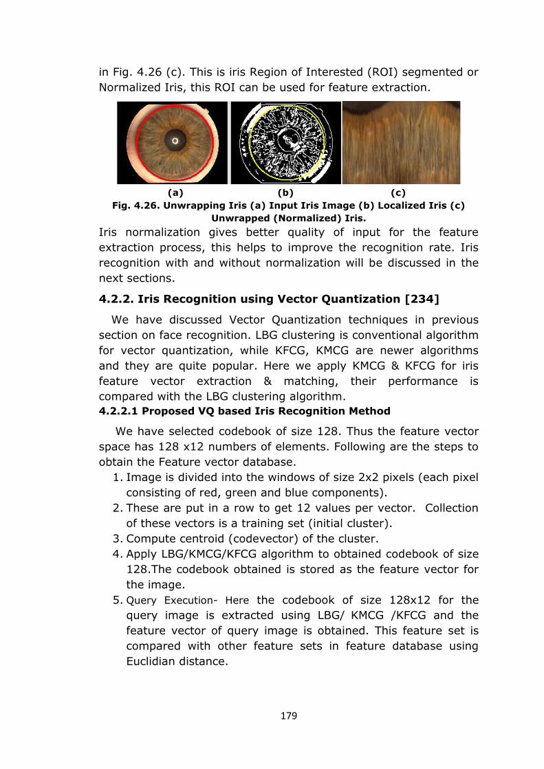
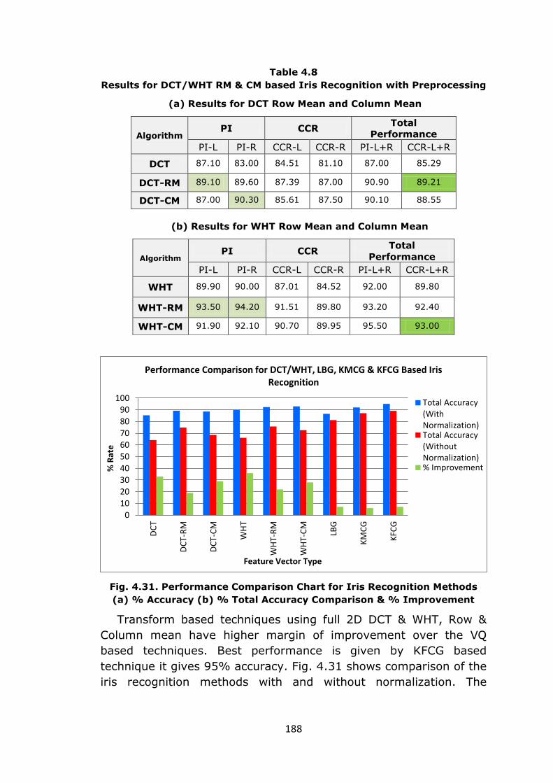
Table 4.8

Results for DCT/WHT RM & CM based Iris Recognition with Preprocessing

(a) Results for DCT Row Mean and Column Mean

Algorithm PI CCR

Total

Performance


DCT 87.10 83.00 84.51 81.10 87.00 85.29

DCT-RM 89.10 89.60 87.39 87.00 90.90 89.21

DCT-CM 87.00 90.30 85.61 87.50 90.10 88.55

(b) Results for WHT Row Mean and Column Mean

Algorithm PI CCR

Total

Performance


WHT 89.90 90.00 87.01 84.52 92.00 89.80

WHT-RM 93.50 94.20 91.51 89.80 93.20 92.40

WHT-CM 91.90 92.10 90.70 89.95 95.50 93.00

Fig. 4.31. Performance Comparison Chart for Iris Recognition Methods

(a) % Accuracy (b) % Total Accuracy Comparison & % Improvement

Transform based techniques using full 2D DCT & WHT, Row &

Column mean have higher margin of improvement over the VQ

based techniques. Best performance is given by KFCG based

technique it gives 95% accuracy. Fig. 4.31 shows comparison of the

iris recognition methods with and without normalization. The

0

10

20

30

40

50

60

70

80

90

100

DC

T

DC

T-R

M

DC

T-C

M

WH

T

WH

T-R

M

WH

T-C

M

LBG

KM

CG

KFC

G

% R

ate

Feature Vector Type

Performance Comparison for DCT/WHT, LBG, KMCG & KFCG Based Iris Recognition

Total Accuracy(WithNormalization)Total Accuracy(WithoutNormalization)% Improvement

189

comparison between total accuracy (combining left & right iris

image) is given.

Table 4.9

Performance Improvement in Total Accuracy (CCR) Achieved due to Iris

Preprocessing & Normalization

Algorithm

Total Accuracy

(With

Normalization)

Total Accuracy

(Without

Normalization)

Improvement

(%)

DCT 85.29 64.21 33

DCT-RM 89.21 74.96 19

DCT-CM 88.55 68.55 29

WHT 89.80 66.10 36

WHT-RM 92.40 75.78 22

WHT-CM 93.00 72.65 28

LBG 86.70 81.25 07

KMCG 92.12 87.10 06

KFCG 95.18 89.10 07

VQ based technique have achieved 6-7% improvements in the

CCR due to iris normalization but the DCT/WHT based techniques

have shown higher improvements. They show improvements in CCR

in the range of 19-36%. DCT row mean based technique has given

19% improvement in CCR while full 2D WHT based technique has

given 36% improvement. This is mainly because the full 2D

transform of only ROI is taken and irrelevant part from iris image is

not considered. The clustering techniques have marginal increase of

6-7%, as these techniques have advantage of clustering data the

irrelevant part (White sclera) is clustered separately has lesser

effect on the final feature vector. The iris preprocessing &

normalization thus clearly gives improvement in the recognition

performance by boosting the performance by at least 6% to

maximum of 36%.

4.3.3 Iris Recognition using Kekre’s Wavelets

Kekre’s wavelets are orthogonal family of wavelets. The wavelets

are fast and can be generated for non-standard size also. Kekre’s

wavelets have been used effectively in section 3.1.2 for texture

feature extraction of fingerprints, in section 3.2.3 & section 3.3.2

for feature extraction of palmprint & finger-knuckle print

respectively. In another extension these wavelets are used for

multiresolution analysis of face images also in section 4.1.2. Here

190

this approach is extended for iris feature vector extraction. As the

iris ROI is rich in texture, the wavelets can be effectively used for

feature vector extraction.

The selected Iris ROI size is scaled to 360 * 180 Pixels. We

divide the ROI into three regions as follows. Region 1 & 2 are non-

overlapping and region 3 is the central 180*180 pixels region

overlapping with region 1 & 2. This arrangement is used for

capturing localized texture information. Each block is the subjected

to multiresolution analysis using Kekre’s wavelet up to three level of

decomposition. Feature vector is extracted in same way as

discussed for face in section 4.1.2 The normalized wavelet

coefficients are stored in the database.

(a)

(b)

Fig. 4.32. Three Blocks for Multiresolution Analysis (a) Iris ROI (360*180

Pixels scaled) (b) Three Regions of 180*180 Pixels each

Table 4.10

Performance Comparison of Kekre’s & Haar Wavelets for Iris Recognition

Wavelets PI CCR

L R L+R L R L+R

Kekre’s

Wavelets 87.40 91.00 93.20 85.20 87.14 90.46

Haar

Wavelets 85.90 88.60 90.50 83.59 86.23 88.75

191

The feature vectors are extracted for enrollment of total 65 users.

Left and Right iris images are considered separately. Per person

three images for left as well as right iris are considered for

enrollment. These images are taken for phoenix iris database [246].

Total 4200 tests were performed for genuine as well as forgery

matching. Kekre’s Wavelets as well as Haar wavelets [228] are used

for feature vector extraction and their performance is compared.

Table 4.10 & Fig. 4.33 summarize the results for wavelet based iris

recognition methods.

Fig. 4.33. Performance Comparison for Kekre’s & Haar Wavelets

(PI & CCR of Kekre’s Wavelets is Higher than Haar Wavelets)

Kekre’s Wavelets have achieved 93.20% PI & CCR of 90.46% for

left + Right iris testing. On the other hand Haar Wavelets have

achieved 90.50% PI& CCR of 88.75% for left + Right iris testing.

This shows that performance of Kekre’s wavelets is better than Haar

wavelets. Combination of left & right iris feature vector is a multi-

instance biometric feature vector and has better PR, EER & CCR

than that of left & right iris.

In the next section Iris recognition using feature vector derived

from Complex Walsh plane in transform domain is discussed,

besides this Hartley transform, DCT, Kekre’s transform & Kekre’s

wavelets are used to generate the complex plane using even & odd

functions of intermediate transform.

87.4 85.9 85.2

83.59

91 88.6

87.14 86.23

93.2

90.5 90.46 88.75

70

80

90

100

Kekre’s Wavelets Haar Wavelets

PI-L CCR-L PI-R CCR-R PI-L+R CCR-L+R

Performance Comparison of Kekre’s & Haar Wavelets for Iris Recognition

192

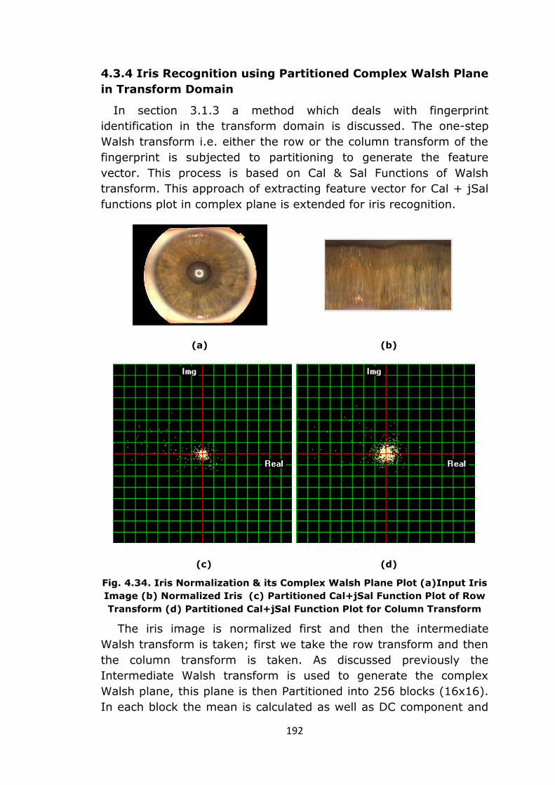
4.3.4 Iris Recognition using Partitioned Complex Walsh Plane

in Transform Domain

In section 3.1.3 a method which deals with fingerprint

identification in the transform domain is discussed. The one-step

Walsh transform i.e. either the row or the column transform of the

fingerprint is subjected to partitioning to generate the feature

vector. This process is based on Cal & Sal Functions of Walsh

transform. This approach of extracting feature vector for Cal + jSal

functions plot in complex plane is extended for iris recognition.

(a) (b)

(c) (d)

Fig. 4.34. Iris Normalization & its Complex Walsh Plane Plot (a)Input Iris

Image (b) Normalized Iris (c) Partitioned Cal+jSal Function Plot of Row

Transform (d) Partitioned Cal+jSal Function Plot for Column Transform

The iris image is normalized first and then the intermediate

Walsh transform is taken; first we take the row transform and then

the column transform is taken. As discussed previously the

Intermediate Walsh transform is used to generate the complex

Walsh plane, this plane is then Partitioned into 256 blocks (16x16).

In each block the mean is calculated as well as DC component and

193

the last Sequency component is together treated as feature vector.

Fig. 4.34 (c) & (d) shows the Partitioned complex Walsh plane for

the Intermediate Walsh row & column transform respectively.

As discussed earlier each plot gives 2S+2 coefficients, we have

256 blocks in each plot, hence one plot gives 514 (256*2 +2)

coefficients for each iris ROI. Similar Feature vector is generated

for density of the points in complex Walsh Plane for each iris ROI

input. This feature vectors are used for enrollment and matching of

the iris.

To test the matching algorithm, 390 iris image samples collected

from 65 persons (6 samples per person, 3 Left & 3 Right iris

images) have been used. Total 3968 different tests are performed.

Equal Error Rate (EER) is evaluated for FAR-FRR analysis as well as

PI & CCR are also calculated. While testing the DC & Sequency

components and its effect on matching is also evaluated. For each

normalized iris ROI input the feature vector is generated in following

variations

1. Row transform feature vector

(Row TRF –L, Row TRF –R)

2. Column transform feature vector

(Col TRF –L, Col TRF –R)

3. Row density feature vector

(Row-Density-L, Row-Density-R)

4. Column density feature vector

(Col-Density-L, Col-Density-R)

5. Fusion of above mention feature vectors with

DC & Sequency components.

(Row TRF + Density + DC SEQ Left,

Row TRF + Density + DC SEQ Right)

6. Final Fusion of Left & Right Iris Feature Vectors- (Fusion)

The fusion is performed by score normalization. The

normalization is performed by weighting the distance by specific

coefficient decided empirically to give proper weightage to each

feature vector. First the Row & Column transform, As well as

Density based feature vectors are fused (Sr. 1 to Sr. 4) along with

DC & Sequency values. This is a multi-algorithmic fusion.

Performance is evaluated for left and right iris separately with

individual as well as multi-algorithmic feature vectors.

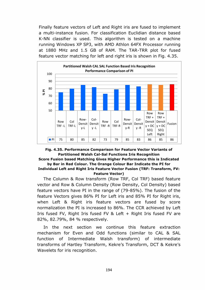
194

Finally feature vectors of Left and Right iris are fused to implement

a multi-instance fusion. For classification Euclidian distance based

K-NN classifier is used. This algorithm is tested on a machine

running Windows XP SP3, with AMD Athlon 64FX Processor running

at 1880 MHz and 1.5 GB of RAM. The TAR-TRR plot for fused

feature vector matching for left and right iris is shown in Fig. 4.35.

Fig. 4.35. Performance Comparison for Feature Vector Variants of

Partitioned Walsh Cal-Sal Functions Iris Recognition

Score Fusion based Matching Gives Higher Performance this is Indicated

by Bar in Red Colour. The Orange Colour Bar Indicate the PI for

Individual Left and Right Iris Feature Vector Fusion (TRF: Transform, FV:

Feature Vector)

The Column & Row transform (Row TRF, Col TRF) based feature

vector and Row & Column Density (Row Density, Col Density) based

feature vectors have PI in the range of (79-85%). The fusion of the

feature Vectors gives 86% PI for Left iris and 85% PI for Right iris,

when Left & Right iris feature vectors are fused by score

normalization the PI is increased to 86%. The CCR achieved by Left

Iris fused FV, Right Iris fused FV & Left + Right Iris fused FV are

82%, 82.79%, 84 % respectively.

In the next section we continue this feature extraction

mechanism for Even and Odd functions (similar to CAL & SAL

function of Intermediate Walsh transform) of intermediate

transforms of Hartley Transform, Kekre’s Transform, DCT & Kekre’s

Wavelets for iris recognition.

RowTRF -L

ColTRF-L

Row-Densit

y-L

Col-Densit

y -L

RowTRF -R

ColTRF-R

Row-Densit

y-R

Col-Densit

y -R

RowTRF +Density + DC

SEQLeft


SEQRight

Fusion

PI 75 80 85 82 73 79 85 83 86 85 86

50

60

70

80

90

100

% P

I

Partitioned Walsh CAL SAL Function Based Iris Recognition Performance Comparison of PI

195

4.3.5. Iris Recognition using Partitioned Complex Plane in

Transform Domain of Hartley Transform, Kekre’s Transform,

Discrete Cosine Transform and Kekre’s Wavelets

The Cal & Sal functions are used to plot (Cal + jSal) points of

intermediate Walsh transform in complex Walsh plane. In previous

section 3.1.4 this study is further extended for other transforms.

Here the same mechanism is used for iris feature vector extraction.

4.3.5.1 Iris Recognition using Partitioned Hartley Plane in

Transform Domain

The intermediate Hartley transform is generated by taking

transform of rows first and then the even and odd rows of this

transforms are used for generating the coefficients for (Even +

jOdd) complex plane plot. These functions are similar to Cal & Sal

functions as used to generate the (Cal + jSal) complex plane. The

complex plane for Hartley transform is shown in Fig. 4.38. Plots for

(Even + jOdd) function points of full finger as well as core point

ROIs are shown. The feature vector as discussed earlier are

extracted from them and used for matching in exactly same way as

discussed for Walsh transform. The performance comparison of the

feature vectors is shown in Fig 4.36.

(a) (b)

Fig. 4.36. Partitioned Complex Hartley Plane of Normalized Iris

(a) Row Transform Function Plot (b) Column Transform Complex

Function Plot

The performance index (PI) of Hartley transforms Even Odd function

based feature vector is in the range of 68% to 88%. Row density

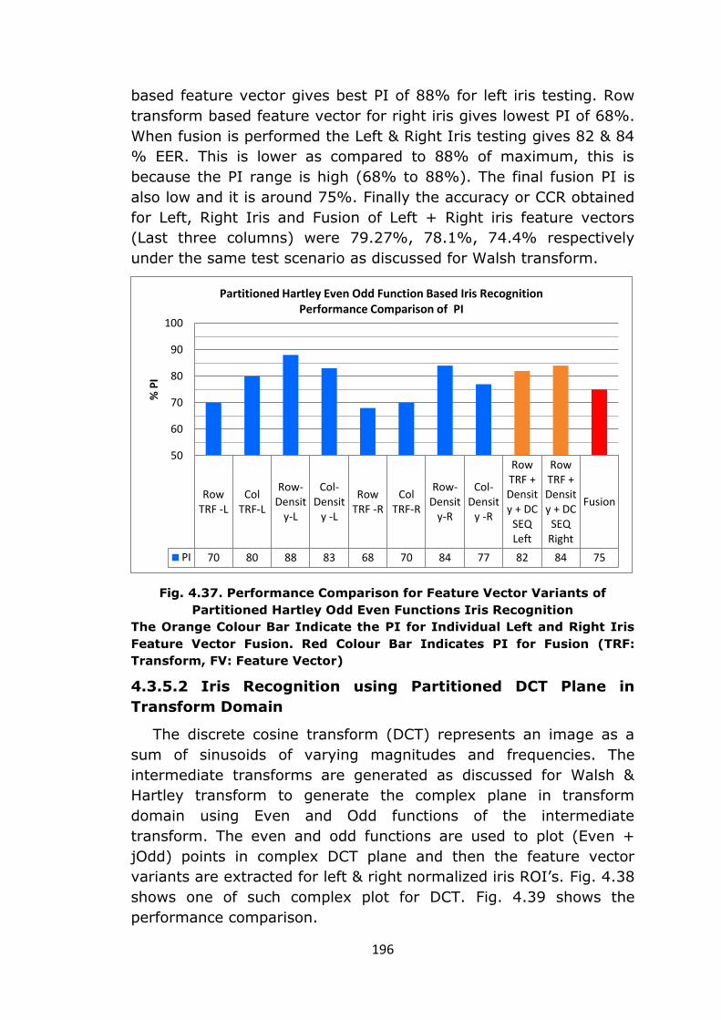
196

based feature vector gives best PI of 88% for left iris testing. Row

transform based feature vector for right iris gives lowest PI of 68%.

When fusion is performed the Left & Right Iris testing gives 82 & 84

% EER. This is lower as compared to 88% of maximum, this is

because the PI range is high (68% to 88%). The final fusion PI is

also low and it is around 75%. Finally the accuracy or CCR obtained

for Left, Right Iris and Fusion of Left + Right iris feature vectors

(Last three columns) were 79.27%, 78.1%, 74.4% respectively

under the same test scenario as discussed for Walsh transform.


Partitioned Hartley Odd Even Functions Iris Recognition

The Orange Colour Bar Indicate the PI for Individual Left and Right Iris

Feature Vector Fusion. Red Colour Bar Indicates PI for Fusion (TRF:

Transform, FV: Feature Vector)

4.3.5.2 Iris Recognition using Partitioned DCT Plane in

Transform Domain

The discrete cosine transform (DCT) represents an image as a

sum of sinusoids of varying magnitudes and frequencies. The

intermediate transforms are generated as discussed for Walsh &

Hartley transform to generate the complex plane in transform

domain using Even and Odd functions of the intermediate

transform. The even and odd functions are used to plot (Even +

jOdd) points in complex DCT plane and then the feature vector

variants are extracted for left & right normalized iris ROI’s. Fig. 4.38

shows one of such complex plot for DCT. Fig. 4.39 shows the

performance comparison.

RowTRF -L

ColTRF-L

Row-Densit

y-L

Col-Densit

y -L

RowTRF -R

ColTRF-R

Row-Densit

y-R

Col-Densit

y -R


SEQLeft


SEQRight

Fusion

PI 70 80 88 83 68 70 84 77 82 84 75

50

60

70

80

90

100

% P

I

Partitioned Hartley Even Odd Function Based Iris Recognition Performance Comparison of PI

197

(a) (b)

Fig. 4.38. Partitioned Complex DCT Plane of Normalized Iris


Function Plot


Partitioned DCT Odd Even Functions Iris Recognition




Feature Vector)

The fusion of feature vectors gives 79 & 80% PI for Left & Right

iris. The final fusion gives improvement in PI, the fusion based

feature vector gives 83% PI. The CCR’s achieved are 78.27, 78.95

& 81.52% for Left iris, Right iris & Fusion based feature vectors.

RowTRF -L

ColTRF-L

Row-Densit

y-L

Col-Densit

y -L

RowTRF -R

ColTRF-R

Row-Densit

y-R

Col-Densit

y -R


SEQLeft


SEQRight

Fusion

PI 74 78 82 71 75 77 83 70 79 80 83

50

60

70

80

90

100

% P

I

Partitioned DCT Even Odd Function Based Iris Recognition Performance Comparison of PI

198

4.3.5.3 Iris Recognition using Partitioned Kekre’s Transform

Plane in Transform Domain

(a) (b)

Fig. 4.40. Partitioned Complex Kekre’s Transform Plane of Normalized

Iris (a) Row Transform Function Plot (b) Column Transform Complex

Function Plot


Partitioned Kekre’s Transform Odd Even Functions Iris Recognition

The Orange Colour Bar Indicate the PI for Individual Left and Right Iris

Feature Vector Fusion (TRF: Transform, FV: Feature Vector)

Kekre’s transform based testing is also performed using Even

Odd function plot in complex plane. Fig.4.40 shows complex plane

RowTRF -L

ColTRF-L

Row-Densit

y-L

Col-Densit

y -L

RowTRF -R

ColTRF-R

Row-Densit

y-R

Col-Densit

y -R


SEQLeft


SEQRight

Fusion

PI 68 73 83 83 65 69 78 79 78 79 75

50

60

70

80

90

100

% P

I

Partitioned Kekre's Transform Even Odd Function Based Iris Recognition Performance Comparison of PI

199

for Even Odd Function plot of Kekre’s Transform. The feature

vectors for Left & Right iris give PI in the range of 65 to 83%. Row

& Column density based feature vectors have higher PI, this is

shown in Fig. 4.41. The fusion of the feature vectors for left & right

iris give PI higher than their individual average, we have achieved

78% and 79% PI for left & right iris fusion. However the final fusion

of left & right iris gives lesser PI of 75%. The CCR’s for left iris, right

iris & Left + Right iris fusion are 77.2, 78.01 & 74% respectively.

4.3.5.4 Iris Recognition using Partitioned Kekre’s Wavelet

Plane in Transform Domain

Finally the Kekre’s wavelets and there use for generating

complex plane plot using Even Odd function of intermediate wavelet

transform is discussed here. The intermediate row and column

transform of normalized iris is taken and then the (Even + j Odd)

function points are plotted in complex plane. One such plot is shown

in Fig. 4.42.

(a) (b)

Fig. 4.42. Partitioned Complex Kekre’s Wavelet Plane of Normalized Iris


Function Plot

The performance comparison of the different feature vectors is

given in Fig.4.43. For left & right iris the Performance Index is in the

range of 71 to 79%. When the fusion is performed for the left &

right iris the fused feature vector give PI of 80 & 79%. The final

fusion of left & right iris gives PI of 81%. The PI of left & right iris

fusion is higher as the individual PIs have narrow range of 71-79%

as compared to previous variants. The CCR’s for Left, Right & Left +

Right iris fusion based feature vectors are 80, 77.98 & 80.53%.

200


Partitioned Kekre’s Wavelet Odd Even Functions Iris Recognition




Feature Vector)


Partitioned Complex Plane based Feature Vectors

RowTRF -L

ColTRF-L

Row-Densit

y-L

Col-Densit

y -L

RowTRF -R

ColTRF-R

Row-Densit

y-R

Col-Densit

y -R


SEQLeft


SEQRight

Fusion

PI 74 75 79 78 71 73 79 77 80 79 81

66

68

70

72

74

76

78

80

82%

PI

Partitioned Kekre's Wavelet Even Odd Function Based Iris Recognition Performance Comparison of PI

WalshTransform

HartleyTransform

DCTKekre's

TransformKekre's

Wavelet

Left Iris 82 79.27 78.27 77.2 80

Right Iris 82.79 78.1 78.95 78.01 77.98

Fusion 84 74.4 81.52 74 80.53

68

70

72

74

76

78

80

82

84

86

% C

CR

Sectorized Complex Plane Iris Recognition Testing Summary - % Accuracy (CCR) Comparison

201

In this section iris recognition using Iris recognition using

Partitioned Complex Walsh Plane in transform domain is discussed.

This method is extended for Even Odd functions complex plane plot

of Hartley Transform, DCT, Kekre’s transform & Kekre’s wavelets.

These methods were tested on normalized iris data and the feature

vectors are extracted for left & right iris images of the user iris

database. Individual left & right iris as well as fusion of both the iris

is tested. The summary is given in Fig.4.44.

Walsh transform based feature vectors give best performance.

The fusion of feature vectors of left & right iris give 84% CCR for

Walsh transform. Next best performance is given by Kekre’s

wavelets, 80.53% of CCR is achieved for fusion of iris feature

vectors. In case of Walsh, DCT & Kekre’s Wavelet based testing the

fusion of left & right iris gave higher CCR as compared to individual

testing, but for Hartley & Kekre’s transform the fusion didn’t yielded

higher CCR, in fact the final CCR is lower in these two cases. This is

mainly because the individual feature vectors performance was low

and having higher variations as compared to other transforms.

4.4 Summary

In this chapter two important biometrics, namely Face & Iris are

discussed in detail. Face requires lower degree of user cooperation

while that for iris is high, still face & iris are widely used in

implementation of unimodal & multimodal biometrics systems. We

have implemented face recognition using Gabor Filter based feature

vector, Kekre & Haar Wavelets, VQ method such as LBG, KFCG,

KMCG clustering algorithms. Gabor filter based system is suitable

for low population and has been tested successfully on handheld

devices. Kekre wavelet & VQ based system provide best accuracy

and feasible for real time face recognition. Amongst VQ techniques

KFCG has best performance.

In case of iris recognition systems based on KMCG, KFCG based

Vector Quantization, DCT & WHT, Kekre & Haar Wavelets, Walsh Cal

Sal functions and Even Odd Functions of other transforms are

tested. The systems have advantage that they don’t need

preprocessing of input image and still provide accuracy up to 90%.

Iris normalization and its effect on iris recognition is studied and it

is observed that it gives up to 36% improvement in PI. We have

tested LBG, KFCG & KMCG based VQ techniques for generating

feature vectors. KFCG gives best accuracy. Transform such as DCT

& Walsh (WHT) are applied on plain image as well as its Row &

202

Column Mean (RM & CM). In another variation Partitioned complex

plane of Walsh and other transforms is used for feature vector

extraction, multi algorithmic as well as multi instance iris

recognition systems using these methods are discussed in this

section. Fusion of left & right iris feature vectors gives further

performance improvement. In the next chapter we discuss

handwritten signature recognition and keystrokes dynamics as

biometrics.

4. Face & Iris Recognition - Shodhgangashodhganga.inflibnet.ac.in/bitstream/10603/9044/9/09_chapter...

Documents

Transcript of 4. Face & Iris Recognition - Shodhgangashodhganga.inflibnet.ac.in/bitstream/10603/9044/9/09_chapter...