4 Estuarine Mixing

Initial concepts: tides and salinityTide-resolving modelsTidal-average modelsTracers for model calibrationMixing diagramsResidence timeDual tracers

What is an estuary?

A semi-enclosed coastal body of water which has a free connection with the open sea and within which sea water is measurably diluted with fresh water derived from land drainage (Pritchard, 1952)Where the river meets the oceanLike a river but with tides and salinity gradients

Tidal motionTidal Channel Ocean

Mouth

2ao

Tt

η(t)

Head2ξo

ao = tidal amplitude

2ao = tidal range

Tt = tidal period

2ξo = tidal excursion

Gravitational and centrifugal acceleration (E with M & S)

Ocean range ~ 0.5 m

Coastal waters may have much larger ranges

Equilibrium tide; moon only

Low

M High High

Water surface

E

Low

At any time: 2 high and 2 low tides;

At any location: ~ 2 high and 2 low tides per day

T=6.8d

13.6dS

Combined sun and moon

Lunar month29.5d

27.3d

20.5d

Sun and moon aligned (full and new moon) => spring tide; Sun and moon opposed (1st and 3rd quarters) => neap tide

Because the earth revolves, period of spring-neap cycle = 365d/[(365/27.3)-1] = 29.5 days

Number of full moon’s per year

And because the moon revolves

ME

24.8

24 h

Lunar day

Lunar day = 29.5 d /(29.5 – 1) = 24.8 hours

Dominant (lunar semi-diurnal tidal) period is 12.4 h

Also a diurnal period

Because of the earth’s declination higher latitudes tend to experience a single (diurnal) cycle per rotation

In general a number of tidal constituents are required to compose an accurate tidal signal

“Side” View

“Top” ViewHHL

L

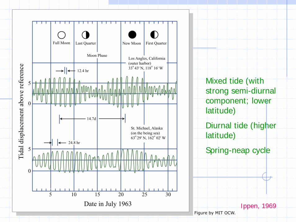
Mixed tide (with strong semi-diurnal component; lower latitude)

Diurnal tide (higher latitude)

Spring-neap cycle

Ippen, 1969

Full Moon Last Quarter New Moon First Quarter

14.7d

12.4 hr

5 10 15 20 25 30

Date in July 1963

0

5

0

5

Tida

l dis

plac

emen

t abo

ve re

fere

nce

St. Michael, Alaska(on the being sea)63o 29' N, 162o 02' W

Los Angles, California(outer harbor)33o 43' N, 118o 16' W

24.8 hr

Moon Phase

Figure by MIT OCW.

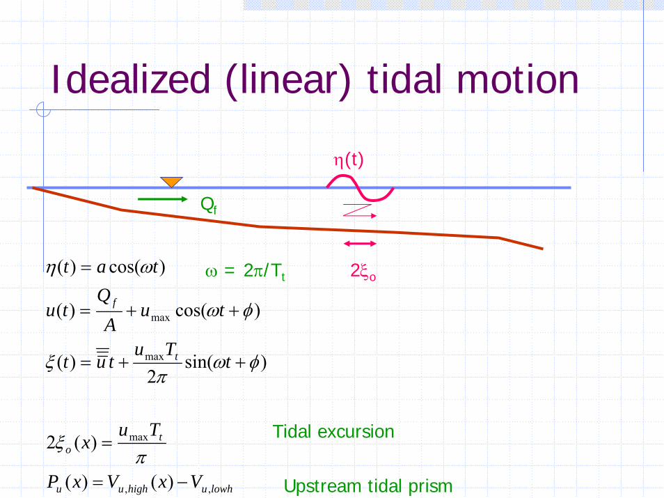
Idealized (linear) tidal motion

η(t)

Qf

lowhuhighuu

to

t

f

VxVxP

Tux

tTu

tut

tuA

Qtu

tat

,,

max

max

max

)()(

)(2

)sin(2

)(

)cos()(

)cos()(

−=

=

++=

++=

=

πξ

φωπ

ξ

φω

ωη 2ξo

Tidal excursion

Upstream tidal prism

ω = 2π/Tt

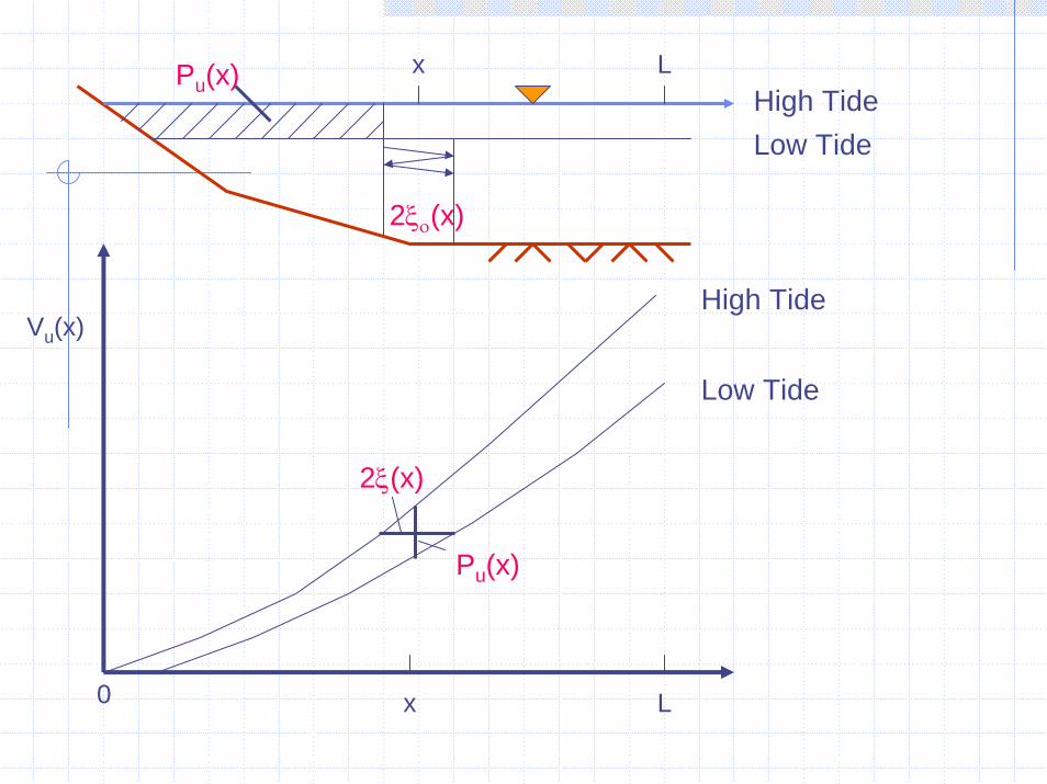
2ξο(x)

Pu(x) x LHigh Tide

Pu(x)

2ξ(x)

Low Tide

High Tide

Low Tide

Vu(x)

0 x L

Now introduce salinityRiver Estuary Ocean

Tidal, Freshwater

Salinity IntrusionQf

+ + +

MouthHead of Tide

S=0

10 20 30

S=35 psu

PSU = practical salinity unit,

an operational definition of salinity (mass fraction: ppt, o/oo or g/kg)

Equation of State (Gill, 1982; ch 6)

3

4

2643

937253

22/3

2

1011)(

108314.4106546.1100227.11072466.5

103875.5102467.8106438.7100899.4824493.0

)(

)9863.3()12963.68(2.508929

9414.28811000)(

)()()(

−

−

−−−

−−−−

⎥⎦⎤

⎢⎣⎡ −=∆

=

−+−=

+−+−=

++=∆

⎥⎦

⎤⎢⎣

⎡−

++

−=

∆+∆+=

xSG

TSSTSS

xCTxTxxB

TxTxTxTxA

CSBSASS

TT

TT

TSSST

ρ

ρ

ρ

ρρρρ (Also pressure at deep depths)

ρ = kg/m3, T in oC, S in PSU (g/kg), TSS in mg/L

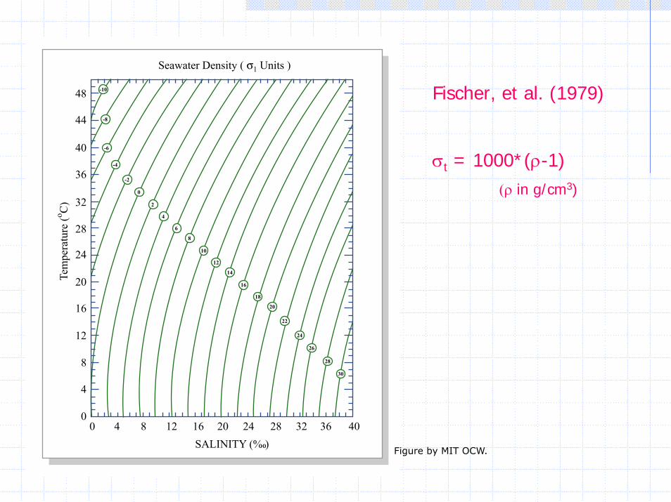
Fischer, et al. (1979)

σt = 1000*(ρ-1)(ρ in g/cm3)

30

28

26

24

22

20

18

16

14

12

10

8

6

4

2

0

-2

-4

-6

-8

-1048

44

40

40

36

36

32

32

28

28

24

24

20

20

16

16

12

12

8

8

4

40

0SALINITY (% )

Tem

pera

ture

(o C)

Seawater Density ( σ1 Units )

Figure by MIT OCW.

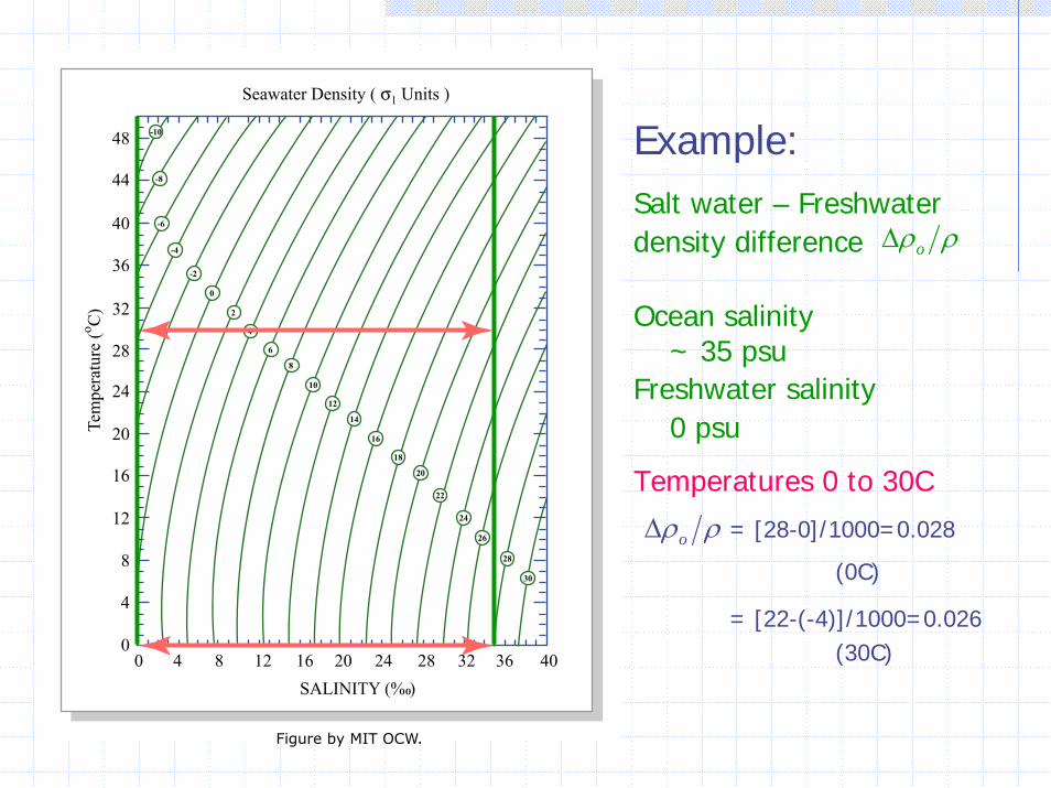
Example:Salt water – Freshwater density difference

Ocean salinity~ 35 psu

Freshwater salinity0 psu

Temperatures 0 to 30C

ρρo∆

ρρo∆ = [28-0]/1000=0.028

(0C)

= [22-(-4)]/1000=0.026 (30C)

30

28

26

24

22

20

18

16

14

12

10

8

6

4

2

0

-2

-4

-6

-8

-1048

44

40

40

36

36

32

32

28

28

24

24

20

20

16

16

12

12

8

8

4

40

0SALINITY (% )

Tem

pera

ture

(o C)

Seawater Density ( σ1 Units )

Figure by MIT OCW.

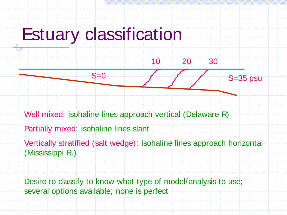
Estuary classification

S=0

10 20 30

S=35 psu

Well mixed: isohaline lines approach vertical (Delaware R)

Partially mixed: isohaline lines slant

Vertically stratified (salt wedge): isohaline lines approach horizontal (Mississippi R.)

Desire to classify to know what type of model/analysis to use; several options available; none is perfect

Estuary classification, cont’dDensimetric Estuary number (Harleman & Abraham, 1966; Thatcher & Harleman, 1972)

hgu

F

TQFP

E

o

od

tf

dtd

)/(

2

ρρ∆=

=periodtidalT

rate;flowfreshwaterQprism;tidalP

t

ft

===

Fd is a densimetric Froude number

differencedensitywaterfreshwatersalt/ρ∆ρdepth;estuaryhvelocity;tidalmaximumu

o

o

−===

Estuary classification, cont’dEstuary Richardson number (Fischer, 1972; 1979)

1

3

~

/

−

∆=

d

t

fo

E

u

WgQR

ρ

ρ

ot 0.71uvelocitytidalRMSuwidth;estuaryW

≅==

R ~ potential energy rate/kinetic energy rate

R < 0.08 well-mixed

0.08 < R < 0.8 partially stratified

0.8 < R vertically stratified (salt wedge)

Example later

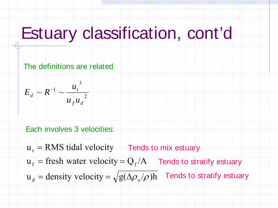
Estuary classification, cont’d

The definitions are related

2

31 ~~

df

td uu

uRE −

Each involves 3 velocities:

)h/g(velocitydensityu

/AQvelocitywaterfreshuvelocitytidalRMSu

od

ff

t

ρρ∆==

=== Tends to mix estuary

Tends to stratify estuary

Tends to stratify estuary

Hanson-Rattray (1966)

Semi-empiricalPredicts

salinity stratification

Velocity stratification

SSSSS sbo )( −=δ

Increases w/ P, decreases w/ Fm

fs /uu

Decreases w/ Fm

d

fm

t

f

uu

F;uu

P ==

=tidal average surf vel /tidal and depth aver vel

P = 3.

3 x 10

-4

10-1

10-2

102 10310-3

P = 3.

3 x 10

-3

P = 3.

3 x 10

-2

P = 3.

3 x 10

-1

P = 10

-3

P = 10

-2

P = 10

-1

F m =

10-4

F m =

10-3

F m =

10-2

F m =

10-1

F m =

1

1

2

10

1 10

δSS0

usuf

Velocity stratification ->

< - Salinity stratification

Figure by MIT OCW.

Tide resolving modelsWell-mixed (1-D) estuary

( ) ∑∑ ′++−

+⎟⎠⎞

⎜⎝⎛

∂∂

∂∂

=∂∂

+∂∂

eiLL

L rrA

ccqxctAE

xAxctu

tc )(1)(

Major difference between river and well-mixed estuary are 1) u is time-varying, 2) EL is constrained by reversing tide.

Look at 2) first

Characteristic dispersion time scales

EL ~ Uc2Tc ~ u*

2Tc

For rivers, two possible time scales, Tc:Ttm ~ B2/ET and Tvm ~ h2/Ez

Ttm >> Tvm => EL ~ u*2 Ttm

(after transverse mixing)

For estuaries, additional possibility: Tc = Tt/2Ttm >> Tt/2 ~ Tvm => EL ~ u*

2 Ttm or u*2 Tt/2

Previous example, B = 100 m, H = 5 m, u = 1 m/s

Tvm = 750 s, Ttm = 34000 s, Tt/2= 22000 s (6.2 h)

(Fischer et al., 1979)

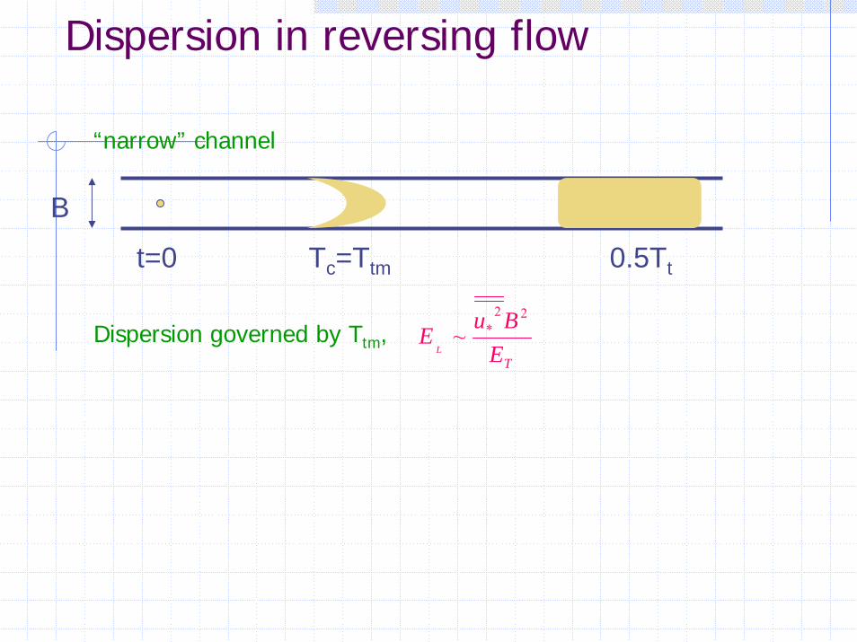
Dispersion in reversing flow

“narrow” channel

B

t=0 Tc=Ttm 0.5Tt

TEBu

EL

22*~Dispersion governed by Ttm,

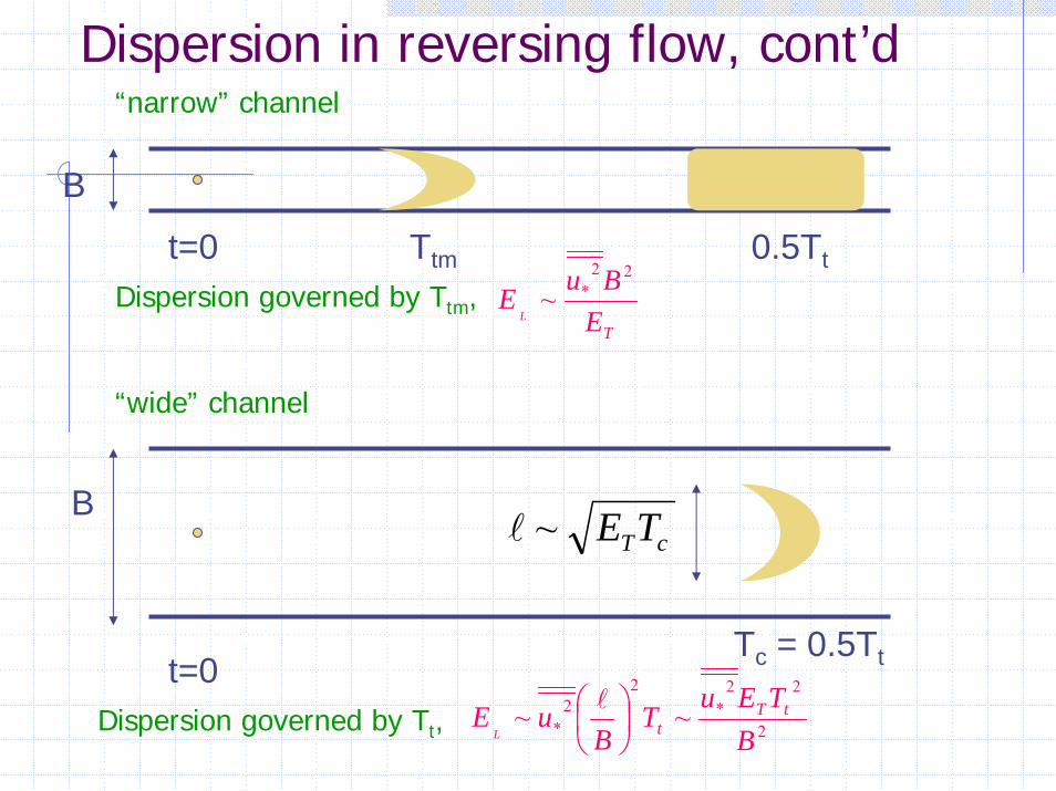
Dispersion in reversing flow, cont’d“narrow” channel

B

Ttm 0.5Ttt=0

TEBu

EL

22*~Dispersion governed by Ttm,

“wide” channel

BcTTE~l

Tc = 0.5Ttt=02

22*

22

* ~~B

TEuT

BuE tT

tL⎟⎠⎞

⎜⎝⎛ l

Dispersion governed by Tt,

Effects of reversing u(t)

Mass continuously injected at x = 0

C

land ocean

High tide

Low tide

x0

2ξo

An actual simulation

Continuous injection at x = 0; output after 30, 400 tidal periods (high slack) and 30.5 and 400.5 tidal cycles (low slack)

ox ξ2/

Harleman, 1971

2.01.51.00.50.0-0.5-1.0-1.5-2.00.0

0.5

1.0

N = 30.0

H.W.S

N = 400.0 N = 400.5

L.W.S

N = 30.5

Figure by MIT OCW.

Tidal-average models

Perhaps we don’t care to resolve intra-tidal time-dependenceStrong non-uniformities prevent resolution of intra-tidal variabilityLong term calculations more efficient with tidal-average time stepHowever, averaging obscures physics

Tidal-average models, cont’dAnalogous, in principle, to time and cross-sectional averaging

uuu ′′′+=Triple bars imply tidal average

ccc ′′′+=

Insert into GE and tidal-average

∑∑ ++⎟⎟⎟

⎠

⎞

⎜⎜⎜

⎝

⎛

∂∂

∂∂

=∂∂

+∂∂

eiL rrxcEA

xAxcu

tc 1 Structurally similar to

equation for river transport => similar solutionsTidal average

velocityTidal average

disp coef

Tidal average dispersionTidal pumping (shown)

Asymmetric ebb (a) & flood (b)Tidal averaging => mean velocity (c)Trans mixing + trans velocity gradients => dispersion!

Similar driversTidal trappingCoriolis + densityDepth-dependent tidal reversal

EL ~ (2ξo)2/Tt

Ebb

Flood

Net

Ebb

Flood

Net

x

x

x

c

A B C

c

c

x

x

x

c

A B C

c

c

c

A B C

c

c

General result

Conservative Tracer; 3 injection locations

Non-conservative tracer; middle location

Non-conservative tracer; 3 locations

Comments

For conservative tracer, c(x)Is independent of xd for x > xd

Decrease with xd for x < xd

If you must pollute, do it downstream (more discussion later)Several specific solutions in notes

Conclusion applies loosely even if not 1-D

Signell, MWRA(1999)

One example

22 /)2(~ xTE toL αξ =

kcdcdcE

dxd

L −⎟⎠⎞

⎜⎝⎛=0

kcdx

cdxdxdcx −α+α=

2

2220

Rectangular channel; no through flowAmq&

="

0 xd L x

Solution

⎥⎦

⎤⎢⎣

⎡−

′′=− −

+−

−

−−

+ 221

221

221

221

),( κκ

κ

κ

κ

ακ ddLd xL

xxxqcxxc x > xd

α+=κ /41 k

⎥⎦

⎤⎢⎣

⎡−=− −

+−

+

+−

221

221

221

221"

),_( κκ

κ

κ

κ

ακ ddLd xL

xxxqcxxc x < xd

WE4-1 Proposed relocation of Gillette’s Intake

Proposal to shorten Fort Point Channel as part of the Big Dig threatened to limit Gillette’s cooling water source

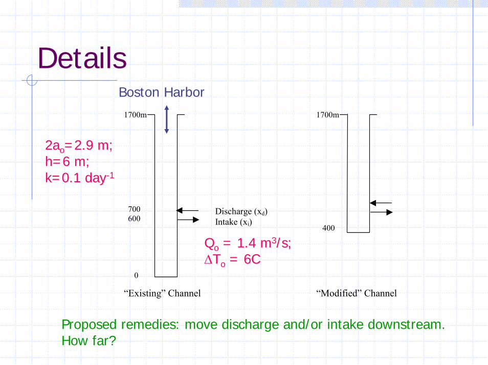
Details

Discharge (xd) Intake (xi)

“Existing” Channel “Modified” Channel

1700m 700 600 0

1700m 400

Qo = 1.4 m3/s; ∆To = 6C

2ao=2.9 m; h=6 m; k=0.1 day-1

Proposed remedies: move discharge and/or intake downstream. How far?

Boston Harbor

Results of analysis

0

0.5

1

1.5

2

2.5

3

0 500 1000 1500 2000Distance (m)

Tem

pera

ture

(C)

Existing

Mod Chan

MC + Disch

Existing: Ti (x=600) ~ 0.8C; Modified: Ti ~ 2.4C

Moving intake 400 m downstream (x=600) yields Ti ~ 0.8C

Moving discharge 300 m downstream (x=900) also yields Ti ~ 0.8C

400 m

xd

Tidal Prism MethodHigh tide

Treats whole channel as single well-mixed box

Mass that leaves on ebb does not returns

Low tideQf

PTm

c

mT

Pc

QTPf

ttp

t

tp

ft

&

&

=

=

=Except for harbors/short channels, this overestimates flushing; underestimates c.

Hence common to “discount” P by defining the effective volume P’ of “clean” water. E.g., P’ = 0.5 P

Formal ways to compute return factor using phase of circulation outside harbor

P = total tidal prismf = “freshness” =(So-Sn)/So

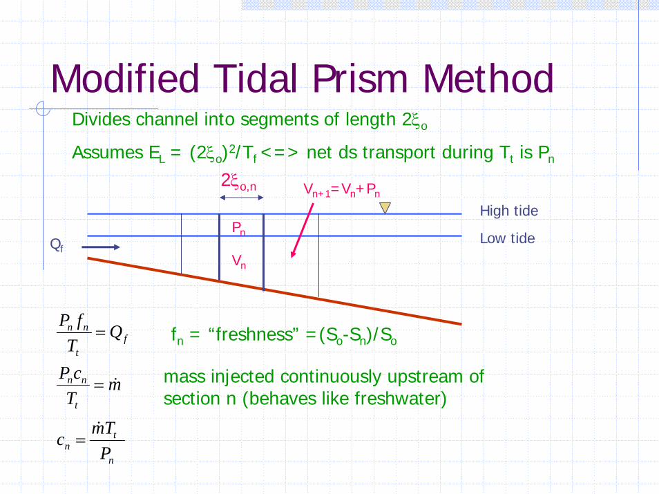
Modified Tidal Prism MethodDivides channel into segments of length 2ξo

Assumes EL = (2ξo)2/Tf <=> net ds transport during Tt is Pn

Pn

Vn

2ξo,n Vn+1=Vn+Pn

n

tn

t

nn

ft

nn

PTmc

mTcP

QT

fP

&

&

=

=

=

High tide

Low tideQf

fn = “freshness” =(So-Sn)/So

mass injected continuously upstream of section n (behaves like freshwater)

Comments

Modified Tidal Prism Method has been modified and re-modified many timesAd-hoc assumption => not always agreement with dataNon-conservative contaminates reduced in concentration by χ

harer

rtkT

/2)1(1

=−−

= −χ

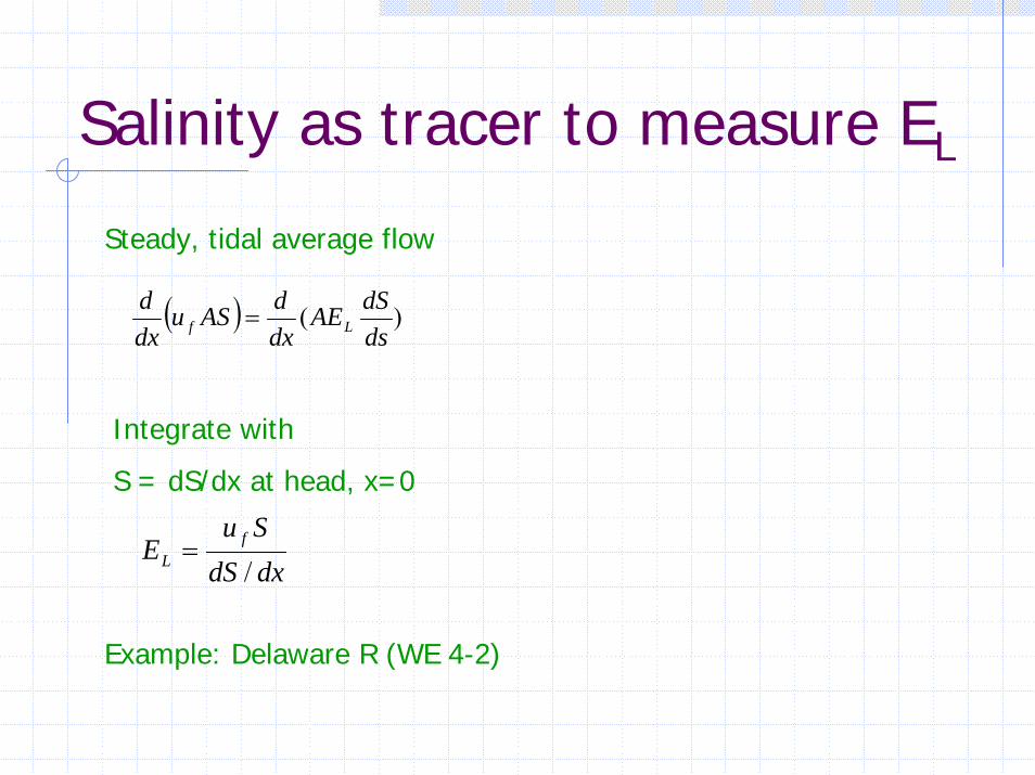
Salinity as tracer to measure EL

Steady, tidal average flow

( ) )(dsdSAE

dxdASu

dxd

Lf =

Integrate with

S = dS/dx at head, x=0

dxdSSu

E fL /

=

Example: Delaware R (WE 4-2)

Measured salinity profiles

Salinity profiles show river to be well-mixed.

Should it be?

What is EL?

Kawabe et al. (1990)

2.0

3.0

4.0

5.0

6.0

7.0

8.0

9.0

10.0

11.0

12.0140.0 120.0 100.0 80.0 60.0 40.0 20.0 0.0

0.018.837.355.974.6

DISTANCE FROM BAY MOUTH (km)

PRES

SUR

E (d

b)

DRBC RIVER MILES

Che

ater

2.04.0

6.0

8.0

10.0

12.0

14.0

16.0

18.0

20.0

22.0

24.0

26.0

28.0

C&

D

2.0

3.0

4.0

5.0

6.0

7.0

8.0

9.0

10.0

11.0

12.0140.0 120.0 100.0 80.0 60.0 40.0 20.0 0.0

0.018.837.355.974.6

DISTANCE FROM BAY MOUTH (km)

PRES

SUR

E (d

b)

DRBC RIVER MILES

Che

ater

2

4

6

8

10

12

14

16

18

20

22

24

26

C&

D

2.0

3.0

4.0

5.0

6.0

7.0

8.0

9.0

10.0

11.0

12.0140.0 120.0 100.0 80.0 60.0 40.0 20.0 0.0

0.018.837.355.974.6

DISTANCE FROM BAY MOUTH (km)

PRES

SUR

E (d

b)

DRBC RIVER MILESC

heat

er

2 4

6

8

10

12

14

16

18

20

22

24

26

C&

D

2.0

3.0

4.0

5.0

6.0

7.0

8.0

9.0

10.0

11.0

12.0140.0 120.0 100.0 80.0 60.0 40.0 20.0 0.0

0.018.837.355.974.6

DISTANCE FROM BAY MOUTH (km)PR

ESSU

RE

(db)

DRBC RIVER MILES

Che

ater

2

4

6

8

10

12

14

16

18

20

22

24

26

C&

D

28.0

October 1986 April 1987

November 1987 April 1988

Figure by MIT OCW.

smx

xSSAQ

dxdSSu

E ffL

/350)20000/)8)(105.1(

)8)(260(/

)/(/

2

4

≅

≅

∆∆≅= Qf = 260 m3/s; A = 1.5x104 m2;

S = 8 psu (80 km);

∆S/∆x = (12-4) psu/20 km (70-90 km)

2.0

3.0

4.0

5.0

6.0

7.0

8.0

9.0

10.0

11.0

12.0140.0 120.0 100.0 80.0 60.0 40.0 20.0 0.0

0.018.837.355.974.6

DISTANCE FROM BAY MOUTH (km)

PRES

SUR

E (d

b)

DRBC RIVER MILES

Che

ater

2

4

6

8

10

12

14

16

18

20

22

24

26

C&

D

Mouth (ocean)Head

~ h (m)

November 1987

Figure by MIT OCW.

Should river be well-mixed?

08.002.01

4000/)260)(10)(025.0(3

3

<≅≅

∆

=t

f

uWQ

gR ρ

ρ

Yes!

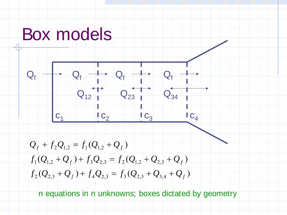
Box models

Qf Qf Qf Qf

c1 c2 c3 c4

Q12 Q23 Q34

)()(

)()(

)(

4,33,233,243,22

3,22,123,232,11

2,112,12

ff

ff

ff

QQQfQfQQf

QQQfQfQQf

QQfQfQ

++=++

++=++

+=+

n equations in n unknowns; boxes dictated by geometry

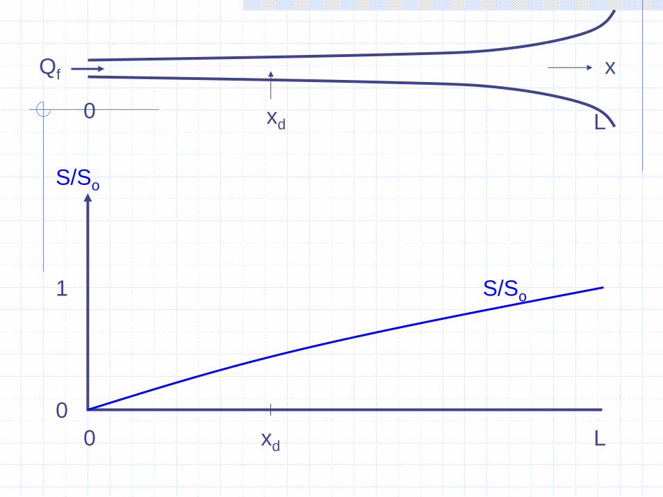
Salinity as direct measure of c

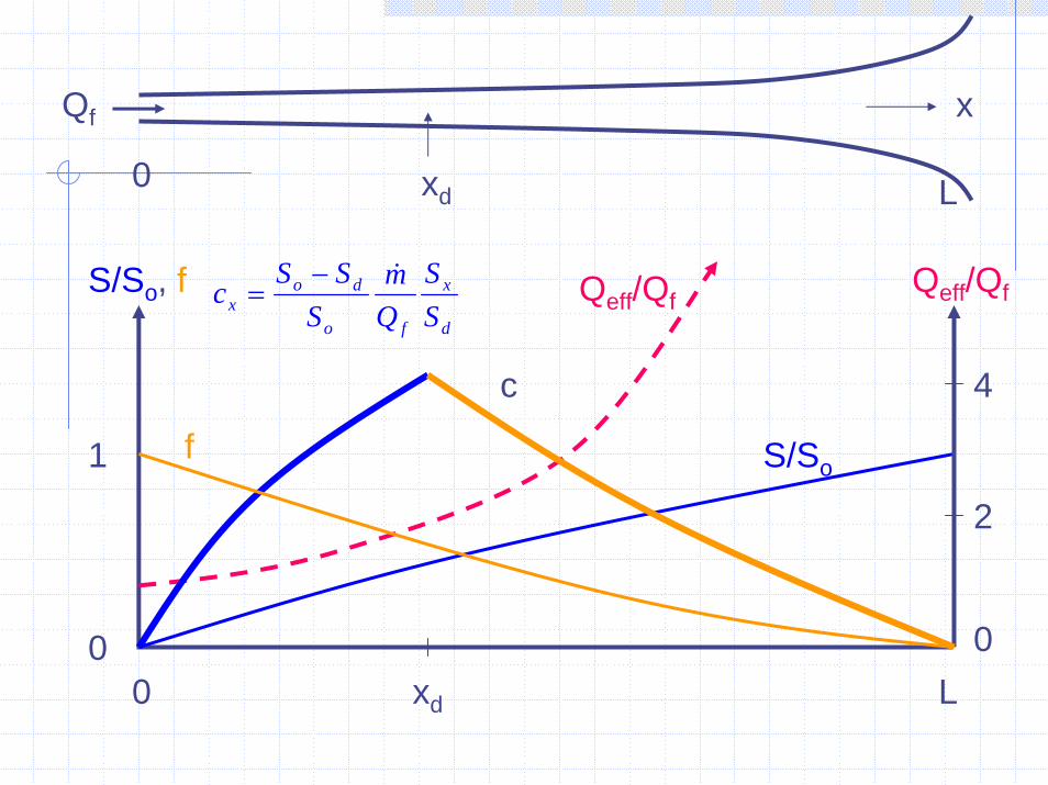
Qf

xd

x

L0

Use measured salinity distribution S(x) resulting from river discharge Qf entering at head (x=0) to infer concentration distribution c(x) of mass entering continuously at downstream location xd.

Qf

xd

x

0 L

S/So

1 S/So

0xd0 L

Qf

xd

x

0 L

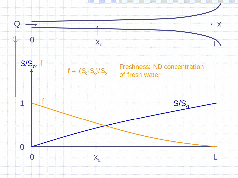
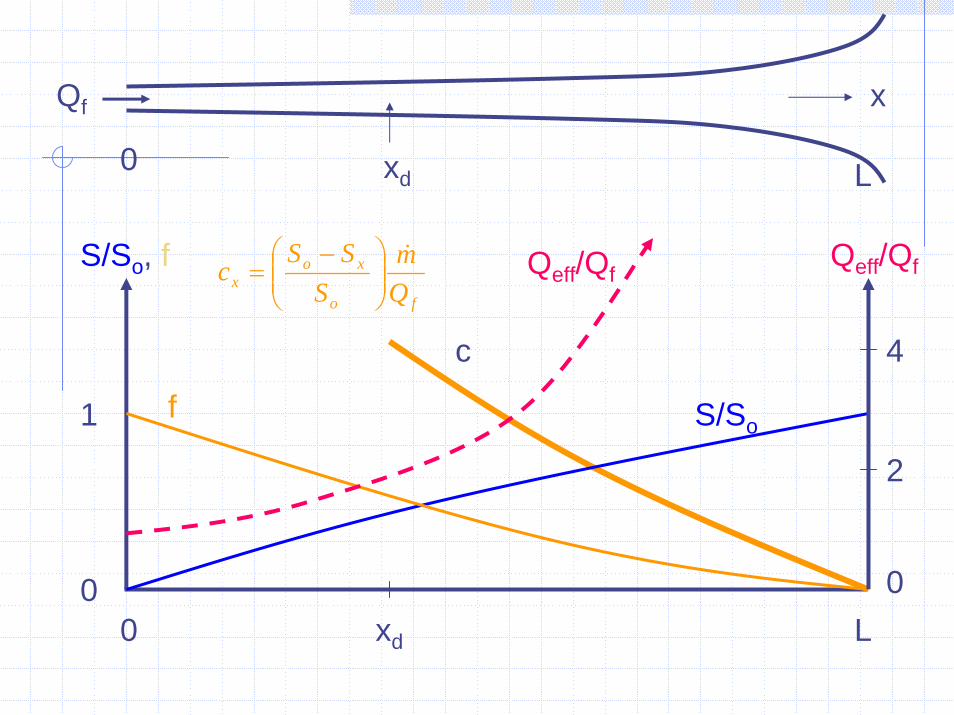
S/So, f Freshness: ND concentration of fresh waterf = (So-Sx)/So

f S/So1

0xd0 L

Qf

xd

x

L0

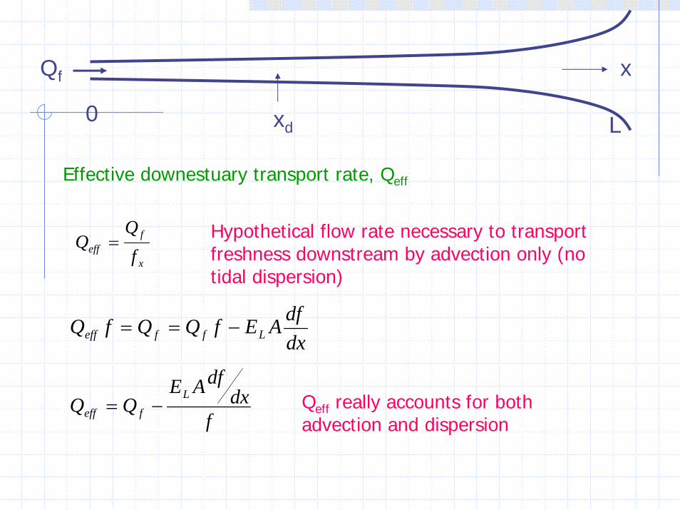
Effective downestuary transport rate, Qeff

x

feff f

QQ = Hypothetical flow rate necessary to transport

freshness downstream by advection only (no tidal dispersion)

dxdfAEfQQfQ Lffeff −==

fdx

dfAEQQ

Lfeff −= Qeff really accounts for both

advection and dispersion

Qf

xd

x

0 L

1

Qeff/QfS/So, f Qeff/Qf

f S/So

Qeff = Qf/f

4

2

00xd0 L

Qf

xd

x

L0

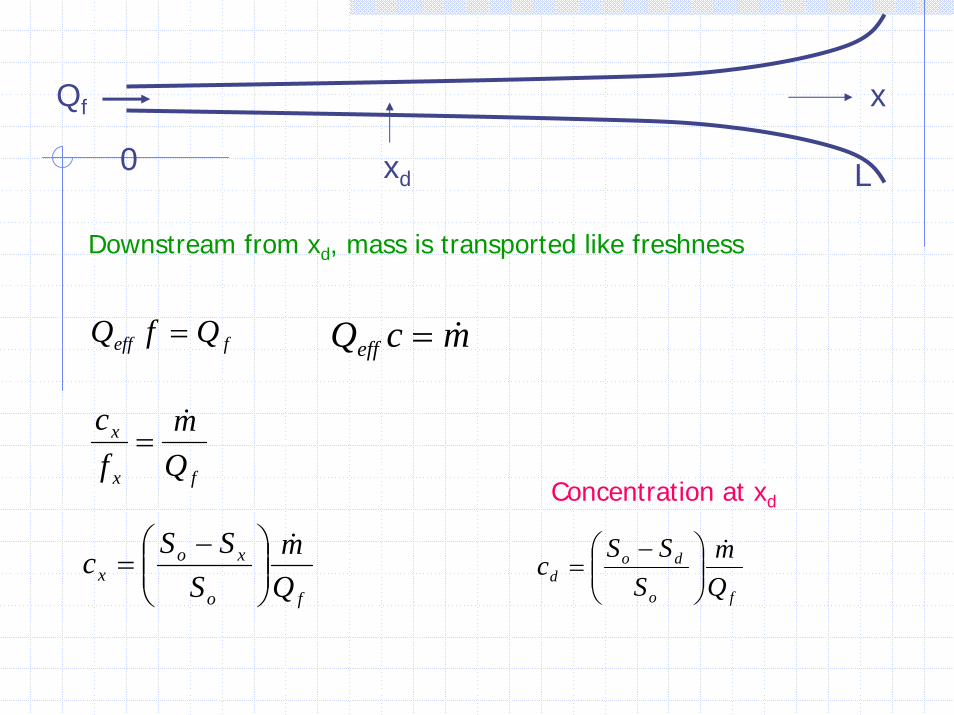
Downstream from xd, mass is transported like freshness

mcQeff &=feff QfQ =

fx

x

Qm

fc &

=

Concentration at xd

fo

xox Q

mS

SSc

&⎟⎟⎠

⎞⎜⎜⎝

⎛ −=

fo

dod Q

mS

SSc

&⎟⎟⎠

⎞⎜⎜⎝

⎛ −=

Qf

xd

x

0 L

1

Qeff/Qf

xd0 L

2

4

0

S/So, f Qeff/Qf

f

c

S/So

fo

xox Q

mS

SSc

&⎟⎟⎠

⎞⎜⎜⎝

⎛ −=

0

Qf

xd

x

L0

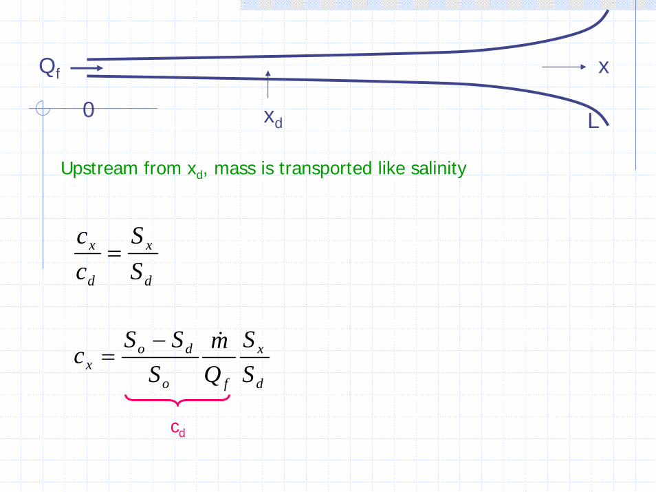
Upstream from xd, mass is transported like salinity

d

x

d

x

SS

cc

=

d

x

fo

dox S

SQm

SSS

c&−

=

cd

Qf

xd

x

0 L

1

Qeff/QfS/So, f Qeff/Qf

f

c

S/So

xd0 L

2

4

d

x

fo

dox S

SQm

SSS

c&−

=

00

(Conservative) Mixing Diagrams

xxx bSac

c

S

−=

Concentration of conservative contaminant discharged at head (using freshness as tracer)

fo

xox Q

mS

SSc

&⎟⎟⎠

⎞⎜⎜⎝

⎛ −=

maxcQma

f

==&

cmax

0So0

aka C-S (or T-S, etc.) diagram, or property-salinity diagram

Uses for Property-S diagrams

Determine end-member concentration and loading (So, Qf known, but not )Identify extraneous sources (we think we know but cmax > co)Distinguish different water massesPredict quality of mixed water massesDetect non-conservative behavior

m&

of cQm =&

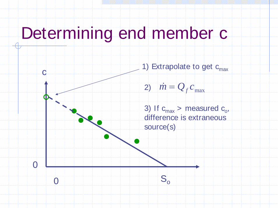
Determining end member c

c

maxcQm f=&

1) Extrapolate to get cmax

2)

3) If cmax > measured co, difference is extraneous source(s)

0So0

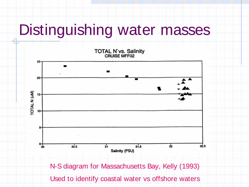
Distinguishing water masses

N-S diagram for Massachusetts Bay, Kelly (1993)

Used to identify coastal water vs offshore waters

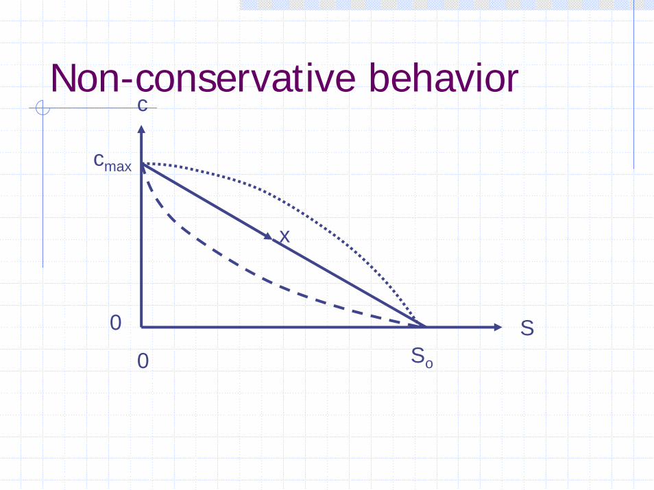
cNon-conservative behavior

x

cmax

0 SSo0

cNon-conservative behavior

x

+

-

cmax

0 SSo0

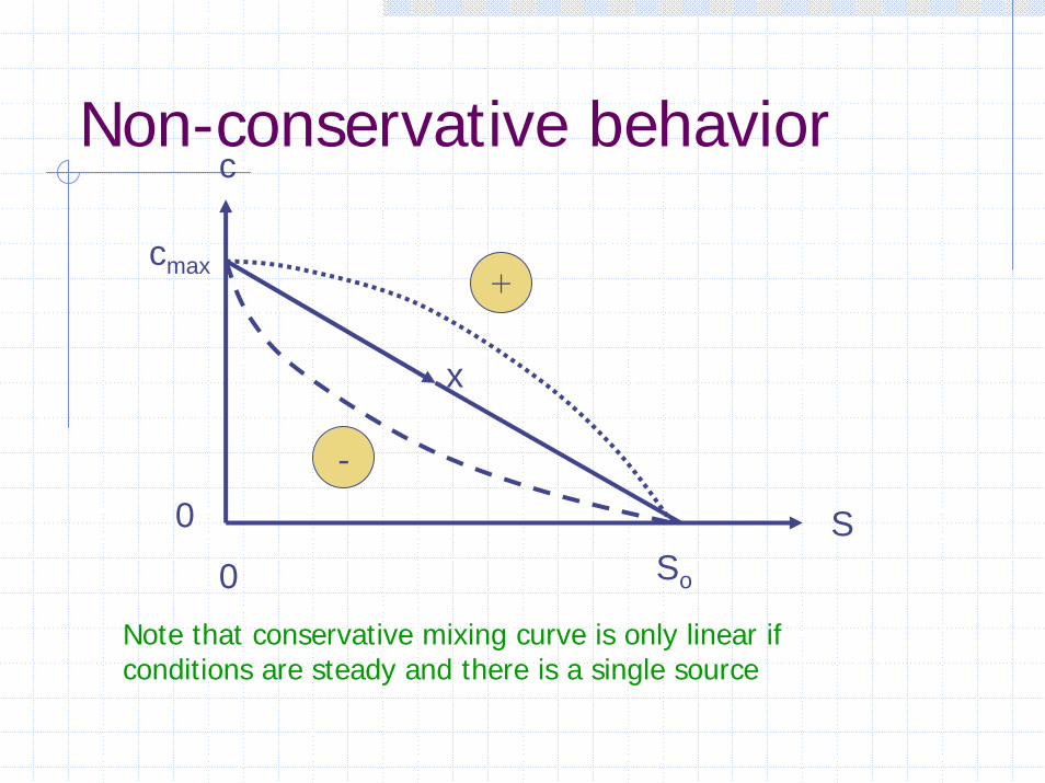
cNon-conservative behavior

x

+

-

cmax

0 SSo0

Note that conservative mixing curve is only linear if conditions are steady and there is a single source

Two conservative sources look like one NC source

c

1

2

0So0

Two conservative sources look like one NC source

c

1

2

1+2

0So0

WE4-2 Nitrate-Salinity diagrams in Delaware R

Transient Conditions

Ciufuentes, et al. (1990)

Solid lines are predictions for conservative tracer & salinity at 4 times (not linear because river flow varies in space and time)

Symbols are data for nitrate & salinity

Why the discrepancy in fall, spring?

200

100

100

200

200

100

100

200

0 16 32

Fall

Summer

Spring

Water

Nitr

ate

(µM

)

Salinity (% )

X

Figure by MIT OCW.

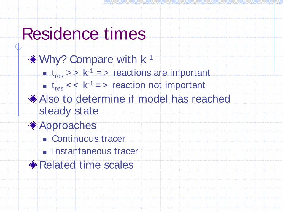
Residence timesWhy? Compare with k-1

tres >> k-1 => reactions are importanttres << k-1 => reaction not important

Also to determine if model has reached steady stateApproaches

Continuous tracerInstantaneous tracer

Related time scales

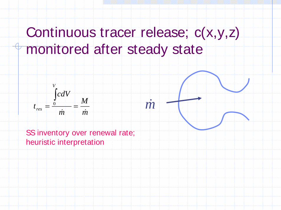
Continuous tracer release; c(x,y,z) monitored after steady state

mM

m

cdVt

V

res &&==

∫0 m&

SS inventory over renewal rate; heuristic interpretation

Types of Tracers

Deliberate tracer (e.g., dye)Tracer of opportunity (e.g. trace metals from WWTP)Freshwater inflow (freshwater fraction approach; residence time sometimes called flushing time)

m&

f

V

res Q

fdVt

∫= 0

Advantages and Disadvantages of each

WE 4-4 Trace metals to calculate residences times for Boston Harbor

dyrdyrkgxmxmkgx

mVctres

4.3)/365/()/107.1()103.6)(/105.2(

5

3236

==

=

−

&

Shea and Kelly, 1992

PAH

PbNi

Cr

Cu

Zn

2500

2000

1500

1000

500

PCBCd

Hg00 20 40 60 80 100 120 140 160 180

Total Load to Harbor (kg/yr)(Thousands)

10 Days

3.4 DaysResidence Time in Boston Harbor

2 Days

Figure by MIT OCW.

CommentsIgnore re-entries (by convention)If multiple sources, tres is average time weighted by mass inflow rateAssumes steady-state, but “fix-ups”applicable to transient loadingResidence time reflects injection location; not property of water body…unless well mixed, in which case:

mVctres &

=constczyxc ==),,(

x

x

x

c

A B C

c

c

x

x

x

c

A B C

c

c

c

A B C

c

c

Tres depends on discharge location

mM

m

cdVt

V

res &&==

∫0

tres A > tres B > tres C

Unit mass

0 t 0 t 0 t

m& m* f*

Instantaneous Release; c(x,y,z,t) monitored over time

11

Rate of injection Mass remaining in system Mass leaving rate

dtdmtf *)(* −= ∫

∞

=0

1)(* dttf

Instantaneous release, cont’d

∫∫∫∞

∞∞∞

+−=−=0

000

)(*** dttmtmtdtdtmdtdtftres&

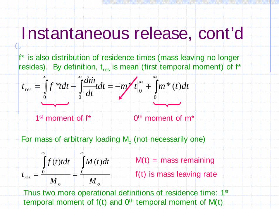
f* is also distribution of residence times (mass leaving no longer resides). By definition, tres is mean (first temporal moment) of f*

1st moment of f* 0th moment of m*

For mass of arbitrary loading Mo (not necessarily one)

oores M

dttM

M

tdttft

∫∫∞∞

== 00

)()( M(t) = mass remaining

f(t) is mass leaving rate

Thus two more operational definitions of residence time: 1st

temporal moment of f(t) and 0th temporal moment of M(t)

WE 4-5 Residence time of CSO effluent in Fort Point ChannelRhodamine WT injected instantaneously at channel head on three dates; results for one survey:

Northern Ave.

Congress St.

Summer St.

Gillette

Dorchester Ave.Broadway

BOS 070

Inner Harbor

Boston

18 ft

18 ft

18 ft

N

100 0 500

Meters

Dye

Figure by MIT OCW.

Adams, et al. (1998)

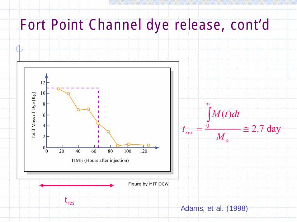
Fort Point Channel dye release, cont’d

day7.2)(

0 ≅=∫∞

ores M

dttMt

tres

12

10

8

6

4

2

00 20 40 60 80 100 120

TIME (Hours after injection)

Tota

l Mas

s of D

ye (K

g)

Figure by MIT OCW.

Adams, et al. (1998)

Comments

f(t) can be obtained from time rate of change of M(t); or from measurements of mass leaving (at mouth)Residence times for continuous and instantaneous releases are equivalentf(t) of f*(t) conveniently used to assess first order mass loss.

∫∞

−= )(* dtetfF kt F = total fraction of mass that leaves

0

WE 4-6 Residence time of bacteria in CSO effluent in Fort Point Channel

Residence time distributions f(t) determined from distributions of m(t).

Indicator bacteria “disappear”(die or settle) at rates of 0.25 to 2 d-1

What fraction of bacteria would disappear for 1990 conditions?

∫∞

−=0

)(* dtetfF kt Fraction (of viable bacteria) that leave

Fraction that are removed within channelF−1

k=2.0 d-1 => F=0.15 (85% removed); k=0.25 d-1=> F=0.55 (45% removed)

40

35

30

25

20

15

10

5

00

50 100 150 200

0.2

0.4

0.6

0.8

1

1.2

1.4

1.6

Time (h)

Mas

s los

s fro

m F

PC (%

/10h

rs)

f*(t) 1990

0.25

0.5

1

2

Figure by MIT OCW.

(Adams et al., 1995)

Relative advantages of 3 approaches?C(V)

Amount of tracer (e.g., dye) required?Effort to dispense?Number of surveys and their spatial extent?Total duration of study?

M (t) f (t)

Mo

t t VInstantaneous Instantaneous Continuous

m

cdVt

V

&

∫= 0

3oM

tdttft

∫∞

= 02

)(

oM

dttMt

∫∞

= 01

)(

Other related time scalesFlushing time use to describe decay of initial concentration distribution (convenient for numerical models); used by EPA for WQ in marinas (see example)Age of water (oceanography): time since tracer entered ocean or was last at surface (complement of tres)Concepts often used interchangeably, but in general different; be careful

Dual TracersUsed to empirically distinguish fate from transport: introduce two tracers (one conservative; one reactive) instantaneously. Applies to any time of water body, but consider well mixed tidal channel

cfc Mk

dtdM

−=

ncncfnc kMMk

dtdM

−−=

Mass of conservative tracer declines due to tidal flushing

Mass of NC tracer declines due to tidal flushing and decay

⎟⎠⎞⎜

⎝⎛−=⎟

⎠⎞⎜

⎝⎛

c

nc

c

ncM

MkMM

dtd Ratio of masses declines due to

decay

kt

oc

nc

c

nc eMM

MM −

⎥⎦⎤

⎢⎣⎡=

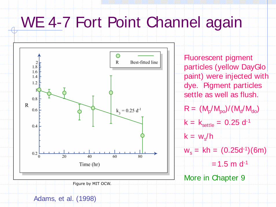
WE 4-7 Fort Point Channel again

Fluorescent pigment particles (yellow DayGlopaint) were injected with dye. Pigment particles settle as well as flush.

R = (Mp/Mpo)/(Md/Mdo)

k = ksettle = 0.25 d-1

k = ws/h

ws = kh = (0.25d-1)(6m)

=1.5 m d-1

More in Chapter 9

0.2

0.4

0.6

0.8

1.21.41.61.8

2

1

R

0 20 40 60 80

Time (hr)

k3 = 0.25 d-1

R Best-fitted line

Figure by MIT OCW.

Adams, et al. (1998)