4. Elementary Graph Algorithms in External Memoryhy460/pdf/AMH/4.pdf4. Elementary Graph Algorithms...

4. Elementary Graph Algorithms in External

Memory∗

Irit Katriel and Ulrich Meyer∗∗

4.1 Introduction

Solving real-world optimization problems frequently boils down to process-ing graphs. The graphs themselves are used to represent and structure rela-tionships of the problem’s components. In this chapter we review external-memory (EM) graph algorithms for a few representative problems:

Shortest path problems are among the most fundamental and also themost commonly encountered graph problems, both in themselves and as sub-problems in more complex settings [21]. Besides obvious applications likepreparing travel time and distance charts [337], shortest path computationsare frequently needed in telecommunications and transportation industries[677], where messages or vehicles must be sent between two geographical lo-cations as quickly or as cheaply as possible. Other examples are complextraffic flow simulations and planning tools [337], which rely on solving a largenumber of individual shortest path problems. One of the most commonlyencountered subtypes is the Single-Source Shortest-Path (SSSP) version: letG = (V,E) be a graph with |V | nodes and |E| edges, let s be a distinguishedvertex of the graph, and c be a function assigning a non-negative real weightto each edge of G. The objective of the SSSP is to compute, for each vertex vreachable from s, the weight dist(v) of a minimum-weight (“shortest”) pathfrom s to v; the weight of a path is the sum of the weights of its edges.

Breadth-First Search (BFS) [554] can be seen as the unweighted version ofSSSP; it decomposes a graph into levels where level i comprises all nodes thatcan be reached from the source via i edges. The BFS numbers also impose anorder on the nodes within the levels. BFS has been widely used since the late1950’s; for example, it is an ingredient of the classical separator algorithmfor planar graphs [507].

Another basic graph-traversal approach is Depth-First Search (DFS) [407];instead of exploring the graph in levels, DFS tries to visit as many graphvertices as possible in a long, deep path. When no edge to an unvisited node∗ Partially supported by the Future and Emerging Technologies programme of

the EU under contract number IST-1999-14186 (ALCOM-FT) and by the DFGgrant SA 933/1-1.

∗∗ Partially supported by the Center of Excellence programme of the EU undercontract number ICAI-CT-2000-70025. Parts of this work were done while theauthor was visiting the Computer and Automation Research Institute of theHungarian Academy of Sciences, Center of Excellence, MTA SZTAKI, Budapest.

U. Meyer et al. (Eds.): Algorithms for Memory Hierarchies, LNCS 2625, pp. 62-84, 2003. Springer-Verlag Berlin Heidelberg 2003

4. Elementary Graph Algorithms in External Memory 63

can be found from the current node then DFS backtracks to the most recentlyvisited node with unvisited neighbor(s) and continues there. Similar to BFS,DFS has proved to be a useful tool, especially in artificial intelligence [177].Another well-known application of DFS is in the linear-time algorithm forfinding strongly connected components [713].

Graph connectivity problems include Connected Components (CC), Bi-connected Components (BCC) and Minimum Spanning Forest (MST/MSF).In CC we are given a graph G = (V,E) and we are to find and enumeratemaximal subsets of the nodes of the graph in which there is a path betweenevery two nodes. In BCC, two nodes are in the same subset iff there aretwo edge-disjoint paths connecting them. In MST/MSF the objective is tofind a spanning tree of G (spanning forest if G is not connected) with aminimum total edge weight. Both problems are central in network design;the obvious applications are checking whether a communications network isconnected or designing a minimum cost network. Other applications for CCinclude clustering, e.g., in computational biology [386] and MST can be usedto approximate the traveling salesman problem within a factor of 1.5 [201].

We use the standard model of external memory computation [755]:There is a main memory of size M and an external memory consisting ofD disks. Data is moved in blocks of size B consecutive words. An I/O-operation can move up to D blocks, one from each disk. Further detailsabout models for memory hierarchies can be found in Chapter 1. We willusually describe the algorithms under the assumption D = 1. In the fi-nal results, however, we will provide the I/O-bounds for general D ≥ 1 aswell. Furthermore, we shall frequently use the following notational short-cuts: scan(x) := O(x/(D · B)), sort(x) := O(x/(D · B) · logM/B(x/B)), andperm(x) := O(minx/D, sort(x)).Organization of the Chapter. We discuss external-memory algorithms forall the problems listed above. In Sections 4.2 – 4.7 we cover graph traversalproblems (BFS, DFS, SSSP) and Sections 4.8 – 4.13 provide algorithms forgraph connectivity problems (CC, BCC, MSF).

4.2 Graph-Traversal Problems: BFS, DFS, SSSP

In the following sections we will consider the classical graph-traversal prob-lems Breadth-First Search (BFS), Depth-First Search (DFS), and Single-Source Shortest-Paths (SSSP). All these problems are well-understood ininternal memory (IM): BFS and DFS can be solved in O(|V | + |E|) time[21], SSSP with nonnegative edge weights requires O(|V | · log |V |+ |E|) time[252, 317]. On more powerful machine models, SSSP can be solved even faster[374, 724].

Most IM algorithms for BFS, DFS, and SSSP visit the vertices of theinput graph G in a one-by-one fashion; appropriate candidate nodes for the

64 Irit Katriel and Ulrich Meyer

next vertex to be visited are kept in some data-structure Q (a queue for BFS,a stack for DFS, and a priority-queue for SSSP). After a vertex v is extractedfrom Q, the adjacency list of v, i.e., the set of neighbors of v in G, is examinedin order to update Q: unvisited neighboring nodes are inserted into Q; thepriorities of nodes already in Q may be updated.

The Key Problems. The short description above already contains the maindifficulties for I/O-efficient graph-traversal algorithms:

(a)Unstructured indexed access to adjacency lists.(b)Remembering visited nodes.(c)(The lack of) Decrease Key operations in external priority-queues.

Whether (a) is problematic or not depends on the sizes of the adjacencylists; if a list contains k edges then it takes Θ(1 + k/B) I/Os to retrieve allits edges. That is fine if k = Ω(B), but wasteful if k = O(1). In spite ofintensive research, so far there is no general solution for (a) on sparse graphs:unless the input is known to have special properties (for example planarity),virtually all EM graph-traversal algorithms require Θ(|V |) I/Os to accessadjacency lists. Hence, we will mainly focus on methods to avoid spendingone I/O for each edge on general graphs1. However, there is recent progressfor BFS on arbitrary undirected graphs [542]; e.g., if |E| = O(|V |), the newalgorithm requires just O(|V |/

√B + sort(|V |)) I/Os. While this is a major

step forward for BFS on undirected graphs, it is currently unclear whethersimilar results can be achieved for undirected DFS/SSSP or BFS/DFS/SSSPon general directed graphs.

Problem (b) can be partially overcome by solving the graph problemsin phases [192]: a dictionary DI of maximum capacity |DI| < M is keptin internal memory; DI serves to remember visited nodes. Whenever thecapacity of DI is exhausted, the algorithms make a pass through the externalgraph representation: all edges pointing to visited nodes are discarded, andthe remaining edges are compacted into new adjacency lists. Then DI isemptied, and a new phase starts by visiting the next element of Q. Thisphase-approach explored in [192] is most efficient if the quotient |V |/|DI| issmall2; O(|V |/|DI| · scan(|V | + |E|)) I/Os are needed in total to performall graph compactions. Additionally, O(|V | + |E|) operations are performedon Q.

As for SSSP, problem (c) is less severe if (b) is resolved by the phase-approach: instead of actually performing Decrease Key operations, severalpriorities may be kept for each node in the external priority-queue; after anode v is dequeued for the first time (with the smallest key) any furtherappearance of v in Q will be ignored. In order to make this work, superfluous1 In contrast, the chapter by Toma and Zeh in this volume (Chapter 5) reviews

improved algorithms for special graph classes such as planar graphs.2 The chapters by Stefan Edelkamp (Chapter 11) and Rasmus Pagh (Chapter 2)

in this book provide more details about space-efficient data-structures.


elements still kept in the EM data structure of Q are marked obsolete rightbefore DI is emptied at the end of a phase; the marking can be done byscanning Q.

Plugging-in the I/O-bounds for external queues, stacks, and priority-queues as presented in Chapter 2 we obtain the following results:

Problem Performance with the phase-approach [192]

BFS, DFS O|V |+

|V |M

· scan(|V |+ |E|)

I/Os

SSSP O|V |+

|V |M

· scan(|V |+ |E|) + sort(|E|)

I/Os

Another possibility is to solve (b) and (c) by applying extra bookkeepingand extra data structures like the I/O-efficient tournament tree of Kumar andSchwabe [485]. In that case the graph traversal can be done in one phase,even if nM .

It turns out that the best known EM algorithms for undirected graphs aresimpler and/or more efficient than their respective counterparts for directedgraphs; due to the new algorithm of [542], the difference for BFS on sparsegraphs is currently as big as Ω(

√B · log |V |).

Problems (b) and (c) usually disappear in the semi-external memory(SEM) setting where it is assumed that M = c · |V | < |E| for some ap-propriately chosen positive constant c: e.g., the SEM model may allow tokeep a boolean array for (b) in internal memory; similarly, a node priorityqueue with Decrease Key operation for (c) could reside completely in IM.

Still, due to (a), the currently best EM/SEM algorithms for BFS, DFSand SSSP requireΩ(|V |+|E|/B) I/Os on general directed graphs. Taking intoconsideration that naive applications of the best IM algorithms in externalmemory cause O(|V | · log |V |+ |E|) I/Os we see how little has been achievedso far concerning general sparse directed graphs. On the other hand, it is per-fectly unclear, whether one can do significantly better at all: the best knownlower-bound is only Ω(perm(|V |) + |E|/B) I/Os (by the trivial reductions oflist ranking to BFS, DFS, and SSSP).

In the following we will present some one-pass approaches in more detail.In Section 4.3 we concentrate on algorithms for undirected BFS. Section 4.4introduces I/O-efficient Tournament Trees; their application to undirectedEM SSSP is discussed in Section 4.5. Finally, Section 4.6 provides traversalalgorithms for directed graphs.


4.3 Undirected Breadth-First Search

Our exposition of one-pass BFS algorithms for undirected graphs is struc-tured as follows. After some preliminary observations we review the basicBFS algorithm of Munagala and Ranade [567] in Section 4.3.1. Then, inSection 4.3.2, we present the recent improvement by Mehlhorn and Meyer[542]. This algorithm can be seen as a refined implementation of the Muna-gala/Ranade approach. The new algorithm clearly outperforms a previousBFS approach [550], which was the first to achieve o(|V |) I/Os on undi-rected sparse graphs with bounded node degrees. A tricky combination ofboth strategies might help to solve directed BFS with sublinear I/O; see Sec-tion 4.7 for more details.

We restrict our attention to computing the BFS level of each node v,i.e., the minimum number of edges needed to reach v from the source. Forundirected graphs, the respective BFS tree or the BFS numbers (order of thenodes in a level) can be obtained efficiently: in [164] it is shown that eachof the following transformations can be done using O(sort(|V | + |E|)) I/Os:BFS Numbers → BFS Tree → BFS Levels → BFS Numbers.

The conversion BFS Numbers → BFS Tree is done as follows: for eachnode v ∈ V , the parent of v in the BFS tree is the node v′ with BFS numberbfsnum(v′) = min(v,w)∈E bfsnum(w). The adjacency lists can be augmentedwith the BFS numbers by sorting. Another scan suffices to extract the BFStree edges.

As for the conversion BFS Tree→ BFS Levels, an Euler tour [215] aroundthe undirected BFS tree can be constructed and processed using scanning andlist ranking; Euler tour edges directed towards the leaves are assigned a weight+1 whereas edges pointing towards the root get weight −1. A subsequentprefix-sum computation [192] on the weights of the Euler tour yields theappropriate levels.

The last transformation BFS Levels → BFS Numbers proceeds level-by-level: having computed correct numbers for level i, the order (BFS numbers)of the nodes in level i+1 is given as follows: each level-(i+1) node v must bea child (in the BFS tree) of its adjacent level-i node with least BFS number.After sorting the nodes of level i and the edges between levels i and i + 1,a scan provides the adjacency lists of level-(i + 1) nodes with the requiredinformation.

4.3.1 The Algorithm of Munagala and Ranade

We turn to the basic BFS algorithm of Munagala and Ranade [567], MR BFSfor short. It is also used as a subroutine in more recent BFS approaches [542,550]. Furthermore, MR BFS is applied in the deterministic CC algorithm of[567] (which we discuss in Section 4.9).

Let L(t) denote the set of nodes in BFS level t, and let |L(t)| be the num-ber of nodes in L(t). MR BFS builds L(t) as follows: let A(t) := N(L(t−1))


N(b)

N(c)

L(t−2) L(t−1) L(t)

b

c e

d f

s a

acd

abde

acd

b

e

a

d

e

d

e

− dupl.N( L(t−1) ) − L(t−1) − L(t−2)

Fig. 4.1. A phase in the BFS algorithm of Munagala and Ranade [567]. Level L(t)is composed out of the disjoint neighbor vertices of level L(t − 1) excluding thosevertices already existing in either L(t− 2) or L(t− 1).

be the multi-set of neighbor vertices of nodes in L(t − 1); N(L(t − 1)) iscreated by |L(t − 1)| accesses to the adjacency lists, one for each node inL(t− 1). Since the graph is stored in adjacency-list representation, this takesO (|L(t− 1)|+ |N(L(t− 1))|/B) I/Os. Then the algorithm removes dupli-cates from the multi-set A. This can be done by sorting A(t) according tothe node indices, followed by a scan and compaction phase; hence, the du-plicate elimination takes O(sort(|A(t)|) I/Os. The resulting set A′(t) is stillsorted.

Now the algorithm computes L(t) := A′(t)\ L(t−1)∪L(t−2). Fig. 4.1provides an example. Filtering out the nodes already contained in the sortedlists L(t− 1) or L(t− 2) is possible by parallel scanning. Therefore, this stepcan be done using

O(sort

(|N(L(t− 1))|

)+ scan

(|L(t− 1)|+ |L(t− 2)|

))I/Os.

Since∑

t |N(L(t))| = O(|E|) and∑

t |L(t)| = O(|V |), the whole execution ofMR BFS requires O(|V |+ sort(|E|)) I/Os.

The correctness of this BFS algorithm crucially depends on the fact thatthe input graph is undirected. Assume that the levels L(0), . . . , L(t− 1) havealready been computed correctly. We consider a neighbor v of a node u ∈L(t − 1): the distance from s to v is at least t − 2 because otherwise thedistance of u would be less than t−1. Thus v ∈ L(t−2)∪L(t−1)∪L(t) andhence it is correct to assign precisely the nodes in A′(t)\L(t−1)∪L(t−2)to L(t).

Theorem 4.1 ([567]). BFS on arbitrary undirected graphs can be solvedusing O(|V |+ sort(|V |+ |E|)) I/Os.

4.3.2 An Improved BFS Algorithm

The Fast BFS algorithm of Mehlhorn and Meyer [542] refines the approachof Munagala and Ranade [567]. It trades-off unstructured I/Os with increas-ing the number of iterations in which an edge may be involved. Fast BFS


operates in two phases: in a first phase it preprocesses the graph and in asecond phase it performs BFS using the information gathered in the firstphase. We first sketch a variant with a randomized preprocessing. Then weoutline a deterministic version.

The Randomized Partitioning Phase. The preprocessing step parti-tions the graph into disjoint connected subgraphs Si, 0 ≤ i ≤ K, withsmall expected diameter. It also partitions the adjacency lists accordingly,i.e., it constructs an external file F = F0F1 . . .Fi . . .FK−1 where Fi con-tains the adjacency lists of all nodes in Si. The partition is built by choos-ing master nodes independently and uniformly at random with probabilityµ = min1,

√(|V |+ |E|)/(B · |V |) and running a local BFS from all mas-

ter nodes “in parallel” (for technical reasons, the source node s is made themaster node of S0): in each round, each master node si tries to capture all un-visited neighbors of its current sub-graph Si; this is done by first sorting thenodes of the active fringes of all Si (the nodes that have been captured in theprevious round) and then scanning the dynamically shrinking adjacency-listsrepresentation of the yet unexplored graph. If several master nodes want toinclude a certain node v into their partitions then an arbitrary master nodeamong them succeeds. The selection can be done by sorting and scanning thecreated set of neighbor nodes.

The expected number of master nodes is K := O(1 + µ · n) and theexpected shortest-path distance (number of edges) between any two nodes ofa subgraph is at most 2/µ. Hence, the expected total amount of data beingscanned from the adjacency-lists representation during the “parallel partitiongrowing” is bounded by

X := O(∑v∈V

1/µ · (1 + degree(v))) = O((|V |+ |E|)/µ).

The total number of fringe nodes and neighbor nodes sorted and scanned dur-ing the partitioning is at most Y := O(|V |+ |E|). Therefore, the partitioningrequires

O(scan(X) + sort(Y )) = O(scan(|V |+ |E|)/µ+ sort(|V |+ |E|))

expected I/Os.After the partitioning phase each node knows the (index of the) sub-

graph to which it belongs. With a constant number of sort and scanoperations Fast BFS can reorganize the adjacency lists into the formatF0F1 . . .Fi . . .F|S|−1, where Fi contains the adjacency lists of the nodes inpartition Si; an entry (v, w,S(w), fS(w)) from the adjacency list of v ∈ Fi

stands for the edge (v, w) and provides the additional information that w be-longs to subgraph S(w) whose subfile FS(w) starts at position fS(w) within F .The edge entries of each Fi are lexicographically sorted. In total, F occupiesO((|V |+ |E|)/B) blocks of external storage.


The BFS Phase. In the second phase the algorithm performs BFS as de-scribed by Munagala and Ranade (Section 4.3.1) with one crucial difference:Fast BFS maintains an external file H (= hot adjacency lists); it comprisesunused parts of subfiles Fi that contain a node in the current level L(t− 1).Fast BFS initializes H with F0. Thus, initially, H contains the adjacencylist of the root node s of level L(0). The nodes of each created BFS level willalso carry identifiers for the subfiles Fi of their respective subgraphs Si.

When creating level L(t) based on L(t− 1) and L(t− 2), Fast BFS doesnot access single adjacency lists like MR BFS does. Instead, it performs aparallel scan of the sorted lists L(t − 1) and H and extracts N(L(t − 1));In order to maintain the invariant that H contains the adjacency lists of allvertices on the current level, the subfiles Fi of nodes whose adjacency listsare not yet included in H will be merged with H. This can be done by firstsorting the respective subfiles and then merging the sorted set with H usingone scan. Each subfile Fi is added to H at most once. After an adjacency listwas copied to H, it will be used only for O(1/µ) expected steps; afterwards itcan be discarded from H. Thus, the expected total data volume for scanningH is O(1/µ · (|V |+ |E|)), and the expected total number of I/Os to handle Hand Fi isO (µ · |V |+ sort(|V |+ |E|) + 1/µ · scan(|V |+ |E|)). The final resultfollows with µ = min1,

√scan(|V |+ |E|)/|V |.

Theorem 4.2 ([542]). External memory BFS on undirected graphs can besolved using O

(√|V | · scan(|V |+ |E|) + sort(|V |+ |E|)

)expected I/Os.

The Deterministic Variant. In order to obtain the result of Theorem 4.2in the worst case, too, it is sufficient to modify the preprocessing phase ofSection 4.3.2 as follows: instead of growing subgraphs around randomly se-lected master nodes, the deterministic variant extracts the subfiles Fi froman Euler tour [215] around a spanning tree for the connected component Cs

that contains the source node s. Observe that Cs can be obtained with thedeterministic connected-components algorithm of [567] usingO((1 + log log(B · |V |/|E|)) · sort(|V |+ |E|)) =O(

√|V | · scan(|V |+ |E|) + sort(|V |+ |E|)) I/Os. The same number of I/Os

suffices to compute a (minimum) spanning tree Ts for Cs [60].After Ts has been built, the preprocessing constructs an Euler tour around

Ts using a constant number of sort- and scan-steps [192]. Then the tour isbroken at the root node s; the elements of the resulting list can be stored inconsecutive order using the deterministic list ranking algorithm of [192]. Thistakes O(sort(|V |)) I/Os. Subsequently, the Euler tour can be cut into piecesof size 2/µ in a single scan. These Euler tour pieces account for subgraphs Si

with the property that the distance between any two nodes of Si in G is atmost 2/µ− 1. See Fig. 4.2 for an example. Observe that a node v of degree dmay be part of Θ(d) different subgraphs Si. However, with a constant numberof sorting steps it is possible to remove multiple node appearances and makesure that each node of Cs is part of exactly one subgraph Si (actually there


2/µs

1 8 1 5

1 8 5

0 4 2 4

0 4 2

7 4 0 6

7 6

01 3 1 6

3

0

4 6

1

8 3

2 7

5

Fig. 4.2. Using an Euler tour around a spanning tree of the input graph in orderto obtain a partition for the deterministic BFS algorithm.

are special algorithms for duplicate elimination, e.g. [1, 534]). Eventually,the reduced subgraphs Si are used to create the reordered adjacency-listfiles Fi; this is done as in the randomized preprocessing and takes anotherO(sort(|V | + |E|)) I/Os. Note that the reduced subgraphs Si may not beconnected any more; however, this does not matter as our approach onlyrequires that any two nodes in a subgraph are relatively close in the originalinput graph.

The BFS-phase of the algorithm remains unchanged; the modified pre-processing, however, guarantees that each adjacency-list will be part of theexternal set H for at most 2/µ BFS levels: if a subfile Fi is merged withH for BFS level L(t), then the BFS level of any node v in Si is at mostL(t) + 2/µ− 1. Therefore, the adjacency list of v in Fi will be kept in H forat most 2/µ BFS levels.

Theorem 4.3 ([542]). External memory BFS on undirected graphs can besolved using O

(√|V | · scan(|V |+ |E|) + sort(|V |+ |E|)

)I/Os in the worst

case.

4.4 I/O-Efficient Tournament Trees

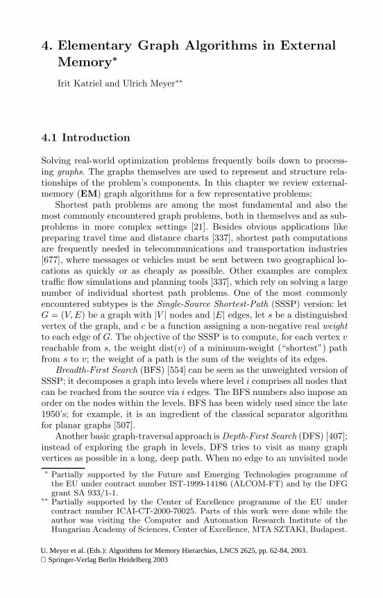
In this section we review a data structure due to Kumar and Schwabe [485]which proved helpful in the design of better EM graph algorithms: the I/O-efficient tournament tree, I/O-TT for short. A tournament tree is a completebinary tree, where some rightmost leaves may be missing. In a figurativesense, a standard tournament tree models the outcome of a k-phase knock-out game between |V | ≤ 2k players, where player i is associated with the i-thleaf of the tree; winners move up in the tree.

The I/O-TT as described in [485] is more powerful: it works as a priorityqueue with the Decrease Key operation. However, both the size of the datastructure and the I/O-bounds for the priority queue operations depend onthe size of the universe from which the entries are drawn. Used in connectionwith graph algorithms, the static I/O-TT can host at most |V | elements with


IndexKey (Priority)

Signals

External Memory

Internal Memory

Signals Elements

M’

M’

M’

M’

M’

M’

M’

M’

M’ M’ M’

M’

M’

M’ 2M’ nn−M’M’+11

Fig. 4.3. Principle of an I/O-efficient tournament tree. Signals are traveling fromthe root to the leaves; elements move in opposite direction.

pairwise disjoint indices in 1, . . . , |V |. Besides its index x, each element alsohas a key k (priority). An element 〈x1, k1〉 is called smaller than 〈x2, k2〉 ifk1 < k2.The I/O-TT supports the following operations:

(i) deletemin: extract the element 〈x, k〉 with smallest key k and replace itby the new entry 〈x,∞〉.

(ii) delete(x): replace 〈x, oldkey〉 by 〈x,∞〉.(iii) update(x,newkey): replace 〈x, oldkey〉 by 〈x,newkey〉 if newkey < oldkey .

Note that (ii) and (iii) do not require the old key to be known. This featurewill help to implement the graph-traversal algorithms of Section 4.5 withoutpaying one I/O for each edge (for example an SSSP algorithm does not have tofind out explicitly whether an edge relaxation leads to an improved tentativedistance).

Similar to other I/O-efficient priority queue data structures (see Chapter 2of Rasmus Pagh for an overview) I/O-TTs rely on the concept of lazy batchedprocessing. Let M ′ = c · M for some positive constant c < 1; the staticI/O-TT for |V | entries only has |V |/M ′ leaves (instead of |V | leaves in thestandard tournament tree). Hence, there areO(log2(|V |/M)) levels. Elementswith indices in the range (i− 1) ·M ′ + 1, . . . , i ·M ′ are mapped to the i-th leaf. The index range of internal nodes of the I/O-TT is given by the


union of the index ranges of their children. Internal nodes of the I/O-TTkeep a list of at least M ′/2 and at most M ′ elements each (sorted accordingto their priorities). If the list of a tree node v contains z elements, thenthey are the smallest z out of all those elements in the tree being mappedto the leaves that are descendants of v. Furthermore, each internal node isequipped with a signal buffer of size M ′. Initially, the I/O-TT stores theelements 〈1,+∞〉, 〈2,+∞〉, . . . , 〈|V |,+∞〉, out of which the lists of internalnodes keep at least M ′/2 elements each. Fig. 4.3 illustrates the principle ofan I/O-TT.

4.4.1 Implementation of the Operations

The operations (i)–(iii) generate signals which serve to propagate informationdown the tree; signals are inserted into the root node, which is kept in internalmemory. When a signal arrives in a node it may create, delete or modify anelement kept in this node; the signal itself may be discarded, altered or remainunchanged. Non-discarded signals are stored until the capacity of the node’sbuffer is exceeded; then they are sent down the tree towards the unique leafnode its associated element is mapped to.

Operation (i) removes an element 〈x, k〉 with smallest key k from the rootnode (in case there are no elements in the root it is recursively refilled fromits children). A signal is sent on the path towards the leaf associated withx in order to reinsert 〈x,+∞〉. The reinsertion takes place at the first treenode on the path with free capacity whose descendents are either empty orexclusively host elements with key infinity.

Operation (ii) is done in a similar way as (i); a delete signal is sent towardsthe leaf node that index x is mapped to; the signal will eventually meet theelement 〈x, oldkey〉 and cause its deletion. Subsequently, the delete signal isconverted into a signal to reinsert 〈x,+∞〉 and proceeds as in case (i).

Finally, the signal for operation (iii) traverses its predefined tree path untileither some node vnewkey with appropriate key range is found or the element〈x, oldkey〉 is met in some node voldkey . In the latter case, if oldkey > newkeythen 〈x,newkey〉 will replace 〈x, oldkey〉 in the list of voldkey ; if oldkey ≤newkey nothing changes. Otherwise, i.e., if 〈x,newkey〉 belongs to a tree nodevnewkey closer to the root than voldkey , then 〈x,newkey〉 will be added to thelist of vnewkey (in case this exceeds the capacity of vnewkey then the largest listelement is recursively flushed to the respective child node of vnewkey using aspecial flush signal). The update signal for update(x,newkey) is altered into adelete signal for 〈x, oldkey〉, which is sent down the tree in order to eliminatethe obsolete entry for x with the old key.

It can be observed that each operation from (i)–(iii) causes at most twosignals to travel all the way down to a leaf node. Overflowing buffers withX > M ′ signals can be emptied using O(X/B) I/Os. Elements moving upthe tree can be charged to signals traveling down the tree. Arguing moreformally along these lines, the following amortized bound can be shown:


Theorem 4.4 ([485]). On an I/O-efficient tournament tree with |V | ele-ments, any sequence of z delete/deletemin/update operations requires at mostO(z/B · log2(|V |/B)) I/Os.

4.5 Undirected SSSP with Tournament Trees

In the following we sketch how the I/O-efficient tournament tree of Section 4.4can be used in order to obtain improved EM algorithms for the single sourceshortest path problem. The basic idea is to replace the data structure Q forthe candidate nodes of IM traversal-algorithms (Section 4.2) by the EMtournament tree. The resulting SSSP algorithm works for undirected graphswith strictly positive edge weights.

The SSSP algorithm of [485] constructs an I/O-TT for the |V | verticesof the graph and sets all keys to infinity. Then the key of the source nodeis updated to zero. Subsequently, the algorithm operates in |V | iterationssimilarly to Dijkstra’s approach [252]: iteration i first performs a deleteminoperation in order to extract an element 〈vi, ki〉; the final distance of theextracted node vi is given by dist(vi) = ki. Then the algorithm issuesupdate(wj , dist(vi) + c(vi, wj)) operations on the I/O-TT for each adjacentedge (vi, wj), vi = wj , having weight c(vi, wj); in case of improvements thenew tentative distances will automatically materialize in the I/O-TT.

However, there is a problem with this simple approach; consider an edge(u, v) where dist(u) < dist(v). By the time v is extracted from the I/O-TT,u is already settled; in particular, after removing u, the I/O-TT replaces theextracted entry 〈u, dist(u)〉 by 〈u,+∞〉. Thus, performing update(u, dist(v)+c(v, u) < ∞) for the edge (v, u) after the extraction of v would reinsert thesettled node u into the set Q of candidate nodes. In the following we sketchhow this problem can be circumvented:

A second EM priority-queue3, denoted by SPQ, supporting a sequence ofz deletemin and insert operations with (amortized) O(z/B · log2(z/B)) I/Osis used in order to remember settled nodes “at the right time”. Initially, SPQis empty. At the beginning of iteration i, the modified algorithm additionallychecks the smallest element 〈u′i, k′i〉 from SPQ and compares its key k′i withthe key ki of the smallest element 〈ui, ki〉 in I/O-TT. Subsequently, onlythe element with smaller key is extracted (in case of a tie, the element inthe I/O-TT is processed first). If ki < k′i then the algorithm proceeds asdescribed above; however, for each update(v, dist(u)+ c(u, v)) on the I/O-TTit additionally inserts 〈u, dist(u) + c(u, v)〉 into the SPQ. On the other hand,if k′i < ki then a delete(u′i) operation is performed on I/O-TT as well and anew phase starts.3 Several priority queue data structures are appropriate; see Chapter 2 for an

overview.


Operation I/O-TT SPQ

. . . 〈u, dist(u)〉, 〈v, ∗〉u =TT deletemin() 〈v, ∗〉

TT update(v, dist(u) + c(u, v)) 〈v, ∗′〉SPQ insert(u, dist(u) + c(u, v)) 〈v, ∗′〉〈u, dist(u) + c(u, v)〉

. . . 〈v, dist(v)〉〈u, dist(u) + c(u, v)〉v =TT deletemin() 〈u, dist(u) + c(u, v)〉

TT update(u, dist(v) + c(u, v)) 〈u, dist(v) + c(u, v)〉〈u, dist(u) + c(u, v)〉. . . 〈u, dist(v) + c(u, v)〉〈u, dist(u) + c(u, v)〉

u =SPQ deletemin() 〈u, dist(v) + c(u, v)〉TT delete(u)

Fig. 4.4. Identifying spurious entries in the I/O-TT with the help of a secondpriority queue SPQ.

In Fig. 4.4 we demonstrate the effect for the previously stated problemconcerning an edge (u, v) with dist(u) < dist(v): after node u is extractedfrom the I/O-TT for the first time, 〈u, dist(u)+ c(u, v)〉 is inserted into SPQ.Since dist(u) < dist(v) ≤ dist(u)+c(u, v), node v will be extracted from I/O-TT while u is still in SPQ. The extraction of v triggers a spurious reinsertionof u into I/O-TT having key dist(v) + c(v, u) = dist(v) + c(u, v) > dist(u) +c(u, v). Thus, u is extracted as the smallest element in SPQ before the re-inserted node u becomes the smallest element in I/O-TT; as a consequence,the resulting delete(u) operation for I/O-TT eliminates the spurious node uin I/O-TT just in time. Extra rules apply for nodes with identical shortestpath distances.

As already indicated in Section 4.2, one-pass algorithms like the one justpresented still require Θ(|V |+(|V |+|E|)/B) I/Os for accessing the adjacencylists. However, the remaining operations are more I/O-efficient: O(|E|) op-erations on the I/O-TT and SPQ add another O(|E|/B · log2(|E|/B)) I/Os.Altogether this amounts to O(|V |+ |E|/B · log2(|E|/B)) I/Os.

Theorem 4.5. SSSP on undirected graphs can be solved usingO(|V |+ |E|/B · log2(|E|/B)) I/Os.

The unpublished full version of [485] also provides a one-pass EM algo-rithm for DFS on undirected graphs. It requires O((|V | + |E|/B) · log2 |V |)I/Os. A different algorithm for directed graphs achieving the same bound willbe sketched in the next section.

4.6 Graph-Traversal in Directed Graphs

The best known one-pass traversal-algorithms for general directed graphs areoften less efficient and less appealing than their undirected counterparts from


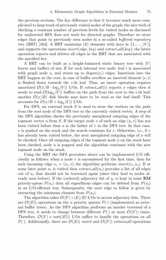
the previous sections. The key difference is that it becomes much more com-plicated to keep track of previously visited nodes of the graph; the nice trick ofchecking a constant number of previous levels for visited nodes as discussedfor undirected BFS does not work for directed graphs. Therefore we storeedges that point to previously seen nodes in a so-called buffered repositorytree (BRT) [164]: A BRT maintains |E| elements with keys in 1, . . . , |V |and supports the operations insert(edge , key) and extract all(key); the latteroperation reports and deletes all edges in the BRT that are associated withthe specified key.

A BRT can be built as a height-balanced static binary tree with |V |leaves and buffers of size B for each internal tree node; leaf i is associatedwith graph node vi and stores up to degree(vi) edges. Insertions into theBRT happen at the root; in case of buffer overflow an inserted element (e, i)is flushed down towards the i-th leaf. Thus, an insert operation requiresamortized O(1/B · log2 |V |) I/Os. If extract all (i) reports x edges then itneeds to read O(log2 |V |) buffers on the path from the root to the i-th leaf;another O(x/B) disk blocks may have to be read at the leaf itself. Thisaccounts for O(x/B + log2 |V |) I/Os.

For DFS, an external stack S is used to store the vertices on the pathfrom the root node of the DFS tree to the currently visited vertex. A step ofthe DFS algorithm checks the previously unexplored outgoing edges of thetopmost vertex u from S. If the target node v of such an edge (u, v) has notbeen visited before then u is the father of v in the DFS tree. In that case,v is pushed on the stack and the search continues for v. Otherwise, i.e., if vhas already been visited before, the next unexplored outgoing edge of u willbe checked. Once all outgoing edges of the topmost node u on the stack havebeen checked, node u is popped and the algorithm continues with the newtopmost node on the stack.

Using the BRT the DFS procedure above can be implemented I/O effi-ciently as follows: when a node v is encountered for the first time, then foreach incoming edge ei = (ui, v) the algorithm performs insert(ei, ui). If atsome later point ui is visited then extract all(ui) provides a list of all edgesout of ui that should not be traversed again (since they lead to nodes al-ready seen before). If the (ordered) adjacency list of ui is kept in some EMpriority-queue P (ui) then all superfluous edges can be deleted from P (ui)in an I/O-efficient way. Subsequently, the next edge to follow is given byextracting the minimum element from P (ui).

The algorithm takes O(|V |+ |E|/B) I/Os to access adjacency lists. Thereare O(|E|) operations on the n priority queues P (·) (implemented as exter-nal buffer trees). As the DFS algorithm performs an inorder traversal of aDFS tree, it needs to change between different P (·) at most O(|V |) times.Therefore, O(|V | + sort(|E|)) I/Os suffice to handle the operations on allP (·). Additionally, there are O(|E|) insert and O(|V |) extract all operations


on the BRT; the I/Os required for them add up to O((|V |+ |E|/B) · log2 |V |)I/Os.

The algorithm for BFS works similarly, except that the stack is replacedby an external queue.

Theorem 4.6 ([164, 485]). BFS and DFS on directed graphs can be solvedusing O((|V |+ |E|/B) · log2 |V |) I/Os.

4.7 Conclusions and Open Problems for Graph Traversal

In the previous sections we presented the currently best EM traversal algo-rithms for general graphs assuming a single disk. With small modifications,the results of Table 4.1 can be obtained for D ≥ 1 disks.

Table 4.1. Graph traversal with D parallel disks.

Problem I/O-Bound

Undir. BFS O

|V | · scan(|V | + |E|) + sort(|V | + |E|)

Dir. BFS, DFS Omin

|V | +

|V |M

· scan(|V | + |E|),

|V | + |E|

D·B· log2 |V |

Undir. SSSP Omin

|V | +

|V |M

· sort(|V | + |E|), |V | + |E|

D·B · log2 |V |

Dir. SSSP O|V | +

|V |M

· sort(|V | + |E|)

One of the central goals in EM graph-traversal is the reduction of un-structured I/O for accessing adjacency-lists. The Fast BFS algorithm ofSection 4.3.2 provides a first solution for the case of undirected BFS. How-ever, it also raises new questions: For example, is Ω(|V |/

√D · B) I/Os a lower

bound for sparse graphs? Can similar results be obtained for DFS or SSSPwith arbitrary nonnegative edge weights? In the following we shortly discussdifficulties concerning possible extensions towards directed BFS.

The improved I/O-bound of Fast BFS stems from partitioning the undi-rected input graph G into disjoint node sets Si such that the distance in Gbetween any two nodes of Si is relatively small. For directed graphs, a par-titioning of that kind may not always exist. It could be beneficial to have alarger number of overlapping node sets where the algorithm accesses just asmall fraction of them. Similar ideas underlie a previous BFS algorithm forundirected graphs with small node degrees [550]. However, there are deepproblems concerning space blow-up and efficiently identifying the “right”partitioning for arbitrary directed graphs. Besides all that, an o(|V |)-I/O


algorithm for directed BFS must also feature novel strategies to rememberpreviously visited nodes. Maybe, for the time being, this additional compli-cation should be left aside by restricting attention to the semi-external case;first results for semi-external BFS on directed Eulerian graphs are given in[542].

4.8 Graph Connectivity: Undirected CC, BCC, andMSF

The Connected Components(CC) problem is to create, for a graph G =(V,E), a list of the nodes of the graph, sorted by component, with a spe-cial record marking the end of each component. The Connected ComponentsLabeling (CCL) problem is to create a vector L of size |V | such that for everyi, j ∈ 1, · · · , |V |, L[i] = L[j] iff nodes i and j are in the same componentof G. A solution to CCL can be converted into a CC output in O(sort(|V |))I/Os, by sorting the nodes according to their component label and addingthe separators.

Minimum Spanning Forest (MSF ) is the problem of finding a subgraph Fof the input graph G such that every connected component in G is connectedin F and the total weight of the edges of F is minimal.

Biconnected Components (BCC) is the problem of finding subsets of thenodes such that u and v are in the same subset iff there are two node-disjointpaths between u and v.

CC and MSF are related, as an MSF yields the connected componentsof the graph. Another common point is that typical algorithms for bothproblems involve reading the adjacency lists of nodes. Reading a node’s ad-jacency list L takes O(scan(|L|)) I/Os, so going over the nodes in an arbi-trary order and reading each node’s adjacency list once requires a total ofO(scan(|E|) + |V |) I/Os. If |V | ≤ |E|/B, the scan(|E|) term dominates.

For both CC and MST, we will see algorithms that have this |V | termin their complexity. Before using such an algorithm, a node reduction stepwill be applied to reduce the number of nodes to at most |E|/B. Then,the |V | term is dominated by the other terms in the complexity. A nodereduction step should have the property that the transformations it performson the graph preserve the solutions to the problem in question. It shouldalso be possible to reintegrate the nodes or edges that were removed intothe solution of the problem for the reduced graph. For both CC and MST,the node reduction step will apply a small number of phases of an iterativealgorithm for the problem. We could repeat such phases until completion, butthat would require Θ (log log |V |) phases, each of which is quite expensive.The combination of a small number, O(log log(|V |B/|E|)), of phases withan efficient algorithm for dense graphs, gives a better complexity. Note thatwhen |V | ≤ |E|, O(sort(|E|) log log(|V |B/|E|)) = O(sort(|E|) log logB).


For BCC, we show an algorithm that transforms the graph and thenapplies CC. BCC is clearly not easier than CC; given an input G = (E, V )to CC, we can construct a graph G′ by adding a new node and connecting itwith each of the nodes of G. Each biconnected component of G′ is the unionof a connected component of G with the new node.

4.9 Connected Components

The undirected BFS algorithm of Section 4.3.1 can trivially be modified tosolve the CCL problem: whenever L(t−1) is empty, the algorithm has spanneda complete component and selects some unvisited node for L(t). It can there-fore number the components, and label each node in L(t) with the currentcomponent number before L(t) is discarded. This adds another O(|V |) I/Os,so the complexity is still O(|V |+ sort(|V |+ |E|)). For a dense graph, where|V | ≤ |E|/B, we have O(|V |+ sort(|V |+ |E|)) = O(sort(|V |+ |E|)). For ageneral graph, Munagala and Ranade [567] suggest to precede the BFS runwith the following node reduction step:

The idea is to find, in each phase, sets of nodes such that the nodes ineach set belong to the same connected component. Among each set a leaderis selected, all edges between nodes of the set are contracted and the set isreduced to its leader. The process is then repeated on the reduced graph.

Algorithm 1. Repeat until |V | ≤ |E|/B:

1. For each node, select a neighbor. Assuming that each node has a uniqueinteger node-id, let this be the neighbor with the smallest id. This par-titions the nodes into pseudotrees (directed graphs where each node hasoutdegree 1).

2. Select a leader from each pseudotree.3. Replace each edge (u, v) in E by an edge (R(u), R(v)), where R(v) is the

leader of the pseudotree v belongs to.4. Remove isolated nodes, parallel edges and self loops.

For Step 1 we sort two copies of the edges, one by source node and one bytarget node, and scan both lists simultaneously to find the lowest numberedneighbor of each node.

For step 2 we note that a pseudotree is a tree with one additional edge.Since each node selected its smallest neighbor, the smallest node in eachpseudotree must be on the pseudotree’s single cycle. In addition, this nodecan be identified by the fact that the edge selected for it goes to a node witha higher ID. Hence, we can scan the list of edges of the pseudoforest, removeeach edge for which the source is smaller than the target, and obtain a forestwhile implicitly selecting the node with the smallest id of each pseudotree asthe leader. On a forest, Step 3 can be implemented by pointer doubling asin the algorithm for list ranking in Chapter 3 with O(sort(|E|)) I/Os. Step 4


requires an additional constant number of sorts and scans of the edges. Thetotal I/Os for one iteration is then O(sort(|E|)). Since each iteration at leasthalves the number of nodes, log2(|V |B/|E|) iterations are enough, for a totalof O(sort(|E|) log(|V |B/|E|)) I/Os.After log2(|V |B/|E|) iterations, we have a contracted graph in which eachnode represents a set of nodes from the original graph. Applying BFS on thecontracted graph gives a component label to each supernode. We then needto go over the nodes of the original graph and assign to each of them thelabel of the supernode it was contracted to. This can be done by sorting thelist of nodes by the id of the supernode that the node was contracted to andthe list of component labels by supernode id, and then scanning both listssimultaneously.The complexity can be further improved by contracting more edges per phaseat the same cost. More precisely, in phase i up to

√Si edges adjacent to each

node will be contracted, where Si = 2(3/2)i(= S

3/2i−1

)(less edges will be con-

tracted only if some nodes have become singletons, in which case they becomeinactive). This means that the number of active nodes at the beginning ofphase i, |Vi|, is at most |V |/Si−1 · Si−2 ≤ |V |/(Si)2/3(Si)4/9 ≤ |V |/Si, andlog log(|V |B/|E|) phases are sufficient to reduce the number of nodes as de-sired.

To stay within the same complexity per phase, phase i is executed on areduced graph Gi, which contains only the relevant edges: those that will becontracted in the current phase. Then |Ei| ≤ |Vi|

√Si. We will later see how

this helps, but first we describe the algorithm:

Algorithm 2. Phase i:

1. For each active node, select up to d =√Si adjacent edges (less if the

node’s degree is smaller). Generate a graph Gi = (Vi, Ei) over the activenodes with the selected edges.

2. Apply log d phases of Algorithm 1 to Gi.3. Replace each edge (u, v) in E by an edge (R(u), R(v)) and remove re-

dundant edges and nodes as in Algorithm 1.

Complexity Analysis. Steps 1 an 3 take O(sort(|E|)) I/Os as in Algo-rithm 1. In Step 2, each phase of Algorithm 1 takes O(sort(|Ei|)) I/Os. With|Ei| ≤ |Vi|

√Si (due to Step 1) and |Vi| ≤ (|V |/Si) (as shown above), this is

O(sort(|V |/

√Si)

)and all log

√Si phases need a total of O(sort(|V |)) I/Os.

Hence, one phase of Algorithm 2 needs O(sort(|E|)) I/Os as before, givinga total complexity of O(sort(|E|) log log(|V |B/|E|)) I/Os for the node re-duction. The BFS-based CC algorithm can then be executed in O(sort(|E|))I/Os.

For D > 1, we perform node reduction phases until |V | ≤ |E|/BD, giving:

Theorem 4.7 ([567]). CC can be solved using

O(sort(|E|) ·max1, log log(|V |BD/|E|)) I/Os.


4.10 Minimum Spanning Forest

An O(|V | + sort(|E|)) MSF algorithm. The Jarnık-Prim [428, 615]MSF algorithm builds the MSF incrementally, one tree at a time. It startswith an arbitrary node and in each iteration, finds the node that is connectedto the current tree by the lightest edge, and adds it to the tree. When theredo not exist any more edges connecting the current tree with unvisited nodes,it means that a connected component of the graph has been spanned. Thealgorithm then selects an arbitrary unvisited node and repeats the processto find the next tree of the forest. For this purpose, the nodes which are notin the MSF are kept in a priority queue, where the priority of a node is theweight of the lightest edge that connects it to the current MSF, and ∞ ifsuch an edge does not exist. Whenever a node v is added to the MSF, thealgorithm looks at v’s neighbors. For each neighbor u which is in the queue,the algorithm compares the weight of the edge (u, v) with the priority of u. Ifthe priority is higher than the weight of the new edge that connects u to thetree, u’s priority is updated. In EM, this algorithm requires at least one I/Oper edge to check the priority of a node, hence the number of I/Os Θ (|E|).

However, Arge et al. [60] pointed out that if edges are kept in the queueinstead of nodes, the need for updating priorities is eliminated. During theexecution of the algorithm, the queue contains (at least) all edges that con-nect nodes in the current MSF with nodes outside of it. It can also containedges between nodes that are in the MSF. The algorithm proceeds as fol-lows: repeatedly perform extract minimum to extract the minimum weightedge (u, v) from the queue. If v is already in the MSF, the edge is discarded.Otherwise, v is included in the MSF and all edges incident to it, except for(u, v), are inserted into the queue. Since each node in the tree inserts all itsadjacent edges, if v is in the MSF, the queue contains two copies of the edge(u, v). Assuming that all edge weights are distinct, after the first copy wasextracted from the queue, the second copy is the new minimum. Therefore,the algorithm can use one more extract-minimum operation to know whetherthe edge should be discarded or not.

The algorithm reads each node’s adjacency list once, with O(|V |+ |E|/B)I/Os. It also performs O(|E|) insert and extract minimum operations onthe queue. By using an external memory priority queue that supports theseoperations in O

(1/B logM/B(N/B)

)I/Os amortized, we get that the total

complexity is O(|V |+ sort(|E|)).Node Reduction for MSF. As in the CC case, we wish to reduce thenumber of nodes to at most |E|/B. The idea is to contract edges that arein the MSF, merging the adjacent nodes into supernodes. The result is areduced graph G′ such that the MSF of the original graph is the union ofthe contracted edges and the edges of the MSF of G′, which can be foundrecursively.


A Boruvka [143] step selects for each node the minimum-weight edge in-cident to it. It contracts all the selected edges, replacing each connected com-ponent they define by a supernode that represents the component, removingall isolated nodes, self-edges, and all but the lowest weight edge among eachset of multiple edges.

Each Boruvka step reduces the number of nodes by at least a factor of two,while contracting only edges that belong to the MSF. After i steps, each su-pernode represents a set of at least 2i original nodes, hence the number of su-pernodes is at most |V |/2i. In order to reduce the number of nodes to |E|/B,log(|V |B/|E|) phases are necessary. Since one phase requires O(sort(|E|))I/Os, this algorithm has complexity ofO(sort(|E|) ·max1, log(|V |B/|E|))).

As with the CC node reduction algorithm, this can be improved by com-bining phases into superphases, where each superphase still needsO(sort(|E|)) I/Os, and reduces more nodes than the basic step. Each su-perphase is the same, except that the edges selected for Ei are not thesmallest numbered

√Si edges adjacent to each node, but the lightest

√Si

edges. Then a superphase which is equivalent to log√si Boruvka steps is

executed with O(sort(|E|)) I/Os. The total number of I/Os for node reduc-tion is O(sort(|E|) ·max1, log log(|V |B/|E|)). The output is the union ofthe edges that were contracted in the node reduction phase and the MSF ofthe reduced graph.

Theorem 4.8 ([567]). MSF can be solved using


4.11 Randomized CC and MSF

We now turn to the randomized MSF algorithm that was proposed by Abello,Buchsbaum and Westbrook [1], which is based on an internal memory algo-rithm that was found by Karger, Klein and Tarjan [445]. As noted above, anMSF algorithm is also a CC algorithm.

Let G = (V,E) be the input graph with edge weights c(e). Let E′ ⊆ E bean arbitrary subset of the edges of G and let F ′ be the MSF of G′ = (V,E′).Denote by WF ′(u, v) the weight of the heaviest edge on the path connectingu and v in F ′. If such a path does not exist, WF ′(u, v) =∞.

Lemma 4.9. For any edge e = (u, v) ∈ E, if w(e) ≥ WF ′(u, v), then thereexists an MSF that does not include e.

The lemma follows immediately from the cycle property: the heaviest edge ofeach cycle is not in the MSF.

The following MSF algorithm is based on Lemma 4.9 [445]:

1. Apply two Boruvka phases to reduce the number of nodes by at least afactor of 4. Call the contracted graph G′.


2. Choose a subgraph H of G′ by selecting each edge independently withprobability p.

3. Apply the algorithm recursively to find the MSF F of H .4. Delete from G′ each edge e = (u, v) for which w(e) > WF ′(u, v). Call the

resulting graph G′′.5. Apply the algorithm recursively to find the MSF F ′ of G′′.6. return the union of the edges contracted in step 1 and the edges of F ′.

Step 1 requires O(sort(|E|)) I/Os and Step 2 an additional O(scan(|E|))I/Os.Step 4 can be done with O(sort(|E|)) I/Os as well [192]. The idea is basedon the MST verification algorithm of King [456], which in turn uses a sim-plification of Komlos’s algorithm for finding the heaviest weight edge on apath in a tree [464]. Since Komlos’s algorithm only works on full branchingtrees4, the MSF F ′ is first converted into a forest of full branching trees F ′′

such that WF ′(u, v) = WF ′′(u, v) and F ′′ has O(|V |) nodes. The conversion isdone as follows: each node of F ′ is a leaf in F ′′. A sequence of Boruvka stepsis applied to F ′ and each step defines one level of each tree in F ′′: the nodesat distance i from the leaves are the supernodes that exist after i Boruvkasteps and the parent of each non-root node is the supernode into which is wascontracted. Since contraction involves at least two nodes, the degree of eachnon-leaf node is at least 2. All Boruvka steps require a total of O(sort(|V |))I/Os.

The next step is to calculate, for each edge (u, v) in G′, the least commonancestor (LCA) of u and v in F ′′. Chiang et al. show that this can be donewith O(sort(|E|)) I/Os [192]. An additional O(sort(|E|)) I/Os are necessaryto construct a list of tuples, one for each edge of G′, of the weight of the edge,its endpoints and the LCA of the endpoints. These tuples are then filteredthrough F ′′ with O((|E|/|V |)sort(|V |)) = O(sort(|E|)) I/Os as follows: eachtuple is sent as a query to the root of the tree and traverses down from ittowards the leaves that represent the endpoints of the edge. When the queryreaches the LCA, it is split into two weight-queries, one continuing towardseach of the endpoints. If a weight query traverses a tree edge which is heavierthan the query edge, the edge is not discarded. Otherwise, it is. To make thisI/O efficient, queries are passed along tree paths using batch filtering [345].This means that instead of traversing the tree from root to leaves for eachquery, a batch of |V | queries is handled at each node before moving on to thenext.

The non-recursive stages then require O(sort(|E|)) I/Os. Karger et al.,have shown that the expected number of edges in G′′ is |V |/p [445]. Thealgorithm includes two recursive calls. One with at most |V |/4 nodes andexpected p|E| edges, and the other with at most |V |/4 nodes and expected|V |/p edges. The total expected I/O complexity is then:

4 A full branching tree is a tree in which all leaves are at the same level and eachnon-leaf node has at least two descendants


t(|E|, |V |) ≤ O(sort(|E|)) + t

(p|E|, |V |

4

)+ t

(|V |p,|V |4

)= O(sort(|E|))

Theorem 4.10 ([1]). MSF and CC can be solved by a randomized algorithmthat uses O(sort(|E|)) I/Os in the expected case.

4.12 Biconnected Components

Tarjan and Vishkin [714] propose a parallel algorithm that reduces BCC toan instance of CC. The idea is to transform the graph G into a graph G′

such that the connected components of G′ correspond to the biconnectedcomponents of G. Each node of G′ represents an edge of G. If two edgese1 and e2 are on the same simple cycle in G, the edge (e1, e2) exists in G′.The problem with this construction is that the graph G′ is very large; it has|E| nodes and up to Ω

(|E|2

)edges. However, they show how to generate a

smaller graph G′′ with the desired properties: instead of including all edgesof G′, first find (any) rooted spanning tree T of G and generate G′′ as the thesubgraph of G′ induced by the edges of T . Formally, we say that two nodesof T are unrelated if neither is a predecessor of the other. G′′ then includesthe edges:

1. (u, v), (x,w) such that (u, v), (x,w) ∈ T , (v, w) ∈ G − T and v, w areunrelated in T .

2. (u, v), (v, w) such that (u, v), (v, w) ∈ T and there exists an edge in Gbetween a descendant of w and a non-descendant of v.

It is not difficult to see that the connected components of G′′ correspond tobiconnected components of G, and that the number of edges in G′′ is O(|E|).

Chiang et al. [192] adapt this algorithm to the I/O model. Finding an arbi-trary spanning tree is obviously not more difficult than finding an MST, whichcan be done with O(sort(|E|) ·max1, log log(|V |BD/|E|)) I/Os (Theorem4.8). To construct G′′, we can use Euler tour and list ranking (Chapter 3) tonumber the nodes by preorder and find the number of descendants of eachnode, followed by a constant number of sorts and scans of the edges to checkthe conditions described above. Hence, the construction of G′′ after we havefound the MSF needs O(sort(|V |)) I/Os. Finding the connected componentsof G′′ has the same complexity as MSF (Theorem 4.7). Deriving the bicon-nected components of G from the connected components of G′′ can then bedone with a constant number of sorts and scans of the edges of G and G′′.

Theorem 4.11 ([192]). BCC can be solved using


Using the result of Theorem 4.10 we get:

Theorem 4.12. BCC can be solved by a randomized algorithm usingO(sort(|E|)) I/Os.


4.13 Conclusion for Graph Connectivity

Munagala and Ranade [567] prove a lower bound of Ω (|E|/|V | · sort(|V |))I/Os for CC, BCC and MSF. Note that |E|/|V | · sort(|V |) = Θ (sort(|E|)).

We have surveyed randomized algorithms that achieve this bound, but thebest known deterministic algorithms have a slightly higher I/O complexity.Therefore, while both deterministic and randomized algorithms are efficient,there still exists a gap between the upper bound and the lower bound in thedeterministic case.

Acknowledgements We would like to thank the participants of the GI-Dagstuhl Forschungsseminar “Algorithms for Memory Hierarchies” for anumber of fruitful discussions and helpful comments on this chapter.

4. Elementary Graph Algorithms in External Memoryhy460/pdf/AMH/4.pdf4. Elementary Graph Algorithms...

Documents

Transcript of 4. Elementary Graph Algorithms in External Memoryhy460/pdf/AMH/4.pdf4. Elementary Graph Algorithms...