
4, 4 DECEMBER, 2016 - · PDF fileVOL. 4, ISSUE 4 – DECEMBER, 2016. 2 ... (Ikhsan, 2007;...
62
1 VOL. 4, ISSUE 4 – DECEMBER, 2016
Transcript of 4, 4 DECEMBER, 2016 - · PDF fileVOL. 4, ISSUE 4 – DECEMBER, 2016. 2 ... (Ikhsan, 2007;...

1
VOL. 4, ISSUE 4 – DECEMBER, 2016

2
Journal of Applied Economics and Business
VOL. 4, ISSUE 4 – DECEMBER, 2016
The Journal of Applied Economics and Business (JAEB – ISSN: 1857-8721) is an international
peer-reviewed, open-access academic journal that publishes original research articles. It
provides a forum for knowledge dissemination on broad spectrum of issues related to applied
economics and business. The journal pays particular attention on contributions of high-quality
and empirically oriented manuscripts supported by various quantitative and qualitative
research methodologies. Among theoretical and applicative contributions, it favors those
relevant to a broad international audience. Purely descriptive manuscripts, which do not
contribute to journal’s aims and objectives are not considered suitable.
JAEB provides a space for academics, researchers and professionals to share latest ideas. It
fosters exchange of attitudes and approaches towards range of important economic and
business topics. Articles published in the journal are clearly relevant to applied economics and
business theory and practice and identify both a compelling practical issue and a strong
theoretical framework for addressing it.
The journal provides immediate open-access to its content on the principle that makes
research freely available to public thus supporting global exchange of knowledge.
JAEB is abstracted and indexed in: DOAJ, EZB, ZDB, Open J-Gate, Google Scholar,
JournalITOCs, New Jour and UlrichsWeb.
Publisher
Education and Novel Technology Research Association
Web: www.aebjournal.org
E-mail: [email protected]

3
Editor-in-Chief
Noga Collins-Kreiner, Department of Geography and Environmental Studies, Center
for Tourism, Pilgrimage & Recreation Research, University of Haifa, Israel
Editorial board
Alexandr M. Karminsky, Faculty of Economics, Higher School of Economics, Russia
Anand Bethapudi, National Institute of Tourism and Hospitality Management, India
Bruno S. Sergi, Department of Economics, Statistics and Geopolitical Analysis of
Territories, University of Mesina, Italy
Dimitar Eftimoski, Department of Economics, Faculty of Administration and
Information Systems Management, St. Kliment Ohridski University, Macedonia
Evangelos Christou, Department of Tourism Management, Alexander Technological
Institute of Thessaloniki, Greece
Irena Ateljevic, Cultural Geography Landscape Center, Wageningen University,
Netherlands
Irena Nančovska Šerbec, Department of mathematics and computing, Faculty of
education, University of Ljubljana, Slovenia
Iskra Christova-Balkanska, Economic Research Institute, Bulgarian Academy of
Sciences, Bulgaria
Joanna Hernik, Faculty of Economics, West Pomeranian University of Technology,
Szczecin, Poland
Karsten Staehr, Tallin School of Economics and Business Administration, Tallin
University of Technology, Estonia
Ksenija Vodeb, Department of Sustainable Tourism Destination, Faculty of Tourism
Studies - TURISTICA, University of Primorska, Slovenia
Kaye Chon, School of Hotel and Tourism Management, the Hong Kong Polytechnic
University, China
Pèter Kovács, Faculty of Economics and Business Administration, University of
Szeged, Hungary
Ramona Rupeika-Apoga, Faculty of Economics and Management, University of
Latvia, Latvia
Renata Tomljenović, Institute for Tourism, Zagreb, Croatia
Valentin Munteanu, Faculty of Economics and Business administration, West
University of Timisoara, Romania

4
Content
Femi Sukmaretiana
The Role of R&D and Location in a Cluster on Total Factor Productivity
Growth of Indonesian Manufacturing 5-20
Monika Trpevska
Future Scenarios and Efficient Transportation 2030 – DB Schenker 21-29
Elena Kosturanova
Tourism Demand in the South-west Planning Region of Macedonia 30-42
Jana Kubicová, Barbora Valková
Factors of the Tax Reporting Compliance of the Slovak Residents 43-62

Journal of Applied Economics and Business
5
THE ROLE OF R&D AND LOCATION IN
A CLUSTER ON TOTAL FACTOR
PRODUCTIVITY GROWTH OF
INDONESIAN MANUFACTURING
Femi Sukmaretiana
Graduate Program in Economics, Faculty of Economics and Business, Universitas Indonesia,
Indonesia
[email protected] / [email protected]
Abstract
Indonesian manufacturing sector plays a key role in the effort to improve economic growth for making the
largest contribution to the total GDP. However, the growth of manufacturing sector is still unstable and the
realization of its growth is still below the expected target. On one hand, examining the total factor productivity
(TFP) growth can help to explain the overall economic growth. On the other hand, R&D and industrial
clustering have been considered as an important factor to improve the efficiency that leads to a higher TFP
growth. This study attempts to examine the source that mainly driven the TFP and the determinant of TFP
growth: particularly the effect of R&D activity and firms’ location in the industrial cluster, since specific
studies that investigate the effect of both factors are still limited. This study uses balanced panel data of
Indonesian large and medium manufacturing firms in the chemical, textile, food and metal sectors for the period
from 2003 to 2013. This study employs stochastic frontier analysis to calculate the efficiency and TFP growth
decomposition. The finding shows that TFP growth on the chemical, metal, food and textile sector are 5.8%,
3.3%, 7.3% and 6.4%, respectively. The technical progress mainly contributes to TFP growth of all four sectors.
Additionally, the result also shows that the R&D activity significantly affects the growth of TFP in the food and
chemical sectors. Furthermore, the industrial cluster positively affects TFP growth in the food and textile and
metal sectors, while it negatively affects the TFP growth in the chemical sector.
Key words
TFP growth, Efficiency, Manufacturing, Indonesia, R&D
INTRODUCTION
The industrial sector plays a key role in the effort to improve the economic growth.
This sector can support the acceleration of GDP growth since it makes the largest
contribution to the total GDP. The government has acknowledged the importance of
this sector by targeting the industrial share at 24 to 30% of total GDP by 2020 and the

Femi Sukmaretiana The Role of R&D and Location in a Cluster on
Total Factor Productivity Growth of Indonesian Manufacturing
6 JOURNAL OF APPLIED ECONOMICS AND BUSINESS, VOL. 4, ISSUE 4 - DECEMBER, 2016, PP. 5-20
average growth rate of the industrial sector to reach 9.5 percent in the period of 2010-
2020 (Ministry of Industry, 2012: 11). However, the growth of the industry is still
unstable, and the realization is still below the expected target. The growth of
medium and large manufacture production index plummeted in 2006 at -1.63%. In
the next period from 2010 to 2015, the growth index slightly increased even though
there was a decrease in 2014 and 2015. In 2015, the share of manufacturing to total
GDP reached 21.5% and the growth of non-oil and gas manufacturing 5.34% in 2014.
Both are still under the targets.
This uneven growth has been triggered many scholars to study what factors that
lead the slowing economic growth and what factors that trigger it. Productivity has
been viewed to have an important role in explaining the overall economic growth.
By examining the total factor productivity (TFP) growth, we can see the other factors
of the growth of output that are not accounted for, by the growth of the inputs in the
production function. The growth accounting method is one way to measure the
sources of growth by distinguishing input growth as one source and TFP growth
reflected in the residual as a second source of growth. Furthermore, there is another
way to analyze the source of TFP growth more deeply by decomposing the TFP.
Unlike the growth accounting method, the decomposition of TFP growth assumes
that not all firms are fully efficient in their production process, which is more
relevant to the real world. Moreover, with the decomposition method we can
identify the contributing factors of TFP growth.
Several studies have been conducted to examine the TFP growth of the Indonesian
manufacturing sector using the decomposition method (Ikhsan, 2007; Margono &
Sharma, 2006; Suyanto et al, 2009). However, none of these studies accounted for
R&D activity and the location of firms in an industrial area as possible determinants
of TFP growth. Griffith et al, (2004) note two channels where the R&D can have an
impact on TFP growth. R&D activity of firms generates product and process
innovation that leads to TFP growth. It also can create knowledge diffusion which
works at three levels: as basic research, as applied research in the private sector and
as applied research in the academic and state research institute. This knowledge
diffusion will affect the long-run growth in the economy as reflected in the
improvement of TFP growth.
Along with R&D, industrial clustering is also considered as an important factor to
improve the efficiency of firms that leads to a higher TFP growth. Porter (1998) notes
that firms can operate more productively as a member of a cluster since it benefits
the members with better access to employees and suppliers, access to specialized
information, and the complementarities as a host of industry linkages among
member firms. Several studies found that the cluster of small-scale industries in
Indonesia has a significant impact on the productivity of the firms (Najib et al, 2011;
Berry et al, 1999). The positive effect from clustering on the productivity of small-
Journal of Applied Economics and Business
7
scale industries has made the Government of Indonesia to advocate the clustering
for larger and medium manufacturing in the national industrial policy (Tijaja &
Faisal, 2014: 14).
Since the specific studies that investigate the effect of R&D activity and the industrial
cluster are still limited, this study aims to fill the gap by examining the role of firms’
R&D activity and the industrial cluster on the efficiency and total factor productivity
growth of the Indonesian manufacturing sector.
LITERATURE REVIEW
The pivotal point of TFP growth in explaining the economic growth can be traced
back to the study of Abramovitz (1956) who argues that the TFP growth might be
interpreted as a proxy to measure the economic growth. Solow (1957) proposes that
the TFP growth might explain the difference in income per capita across countries
and Romer (1990) provides a theoretical study to show that TFP endogenously
explains the economic growth. The study by Klenow and Rodriguez-Clare (1997)
argues that TFP growth represents 90% of the difference of output growth across
nations.
Total factor productivity growth is the residual of the output growth that cannot be
accounted for by inputs growth in the production function. The decomposition of
TFP growth to the components of technical progress, technical efficiency and scale of
firm operation explains the source of economic growth beyond those reflected in the
production function.
In the case of Indonesia, the sharp difference of growth in the manufacturing sector
before and after the economic crisis in the mid 1990’s has led the increasing number
of studies on productivity growth in this sector. Some of the studies estimate the TFP
growth of the manufacturing sector in Indonesia, including a study by Timmer (1999)
that find that annual TFP growth in Indonesian manufacturing during 1975-1999
was 2.8%. Aswincahyono and Hill (2002) note that the average TFP growth of
Indonesian manufacturing during 1975-1993 was 2.3%. The growth increased
between 1976 and 1981, but declined during the period 1981-1993 with negative
growth rate of -4.9% per annum. Margono and Sharma (2006) study the TFP growth
of four sectors of Indonesian manufacturing namely the chemical sector, food sector,
metal sector and textile sector during 1993-2000 using the stochastic frontier model.
They found that the productivity of the chemical, textile and metal sector decreases
in that period but the productivity of chemical sector increases at the rate of 0.5%.
The decomposition method identified that the growth is driven positively by
technical efficiency changes in all four sectors; however, there is a decreasing
technological progress in all four sectors during this period. Ikhsan (2007) studies the
TFP growth in Indonesian manufacturing in the period 1988-2000 considering the

Femi Sukmaretiana The Role of R&D and Location in a Cluster on
Total Factor Productivity Growth of Indonesian Manufacturing
8 JOURNAL OF APPLIED ECONOMICS AND BUSINESS, VOL. 4, ISSUE 4 - DECEMBER, 2016, PP. 5-20
liberalization policies and the economic crisis in 1997. Using the stochastic frontier
analysis with TFP decomposition, the finding showed that TFP grew by 1.5%
between 1988 and 2000. The TFP growth is mostly driven by the technical progress
and there is the negative trend in technical efficiency change reflecting the learning
process of technology adoption that has not been used efficiently.
In analyzing the manufacturing sector, the study of the efficiency of firms is also
important to measure industry performance. The level of efficiency in the industrial
sector indicates how well the firms in that industry can produce maximum output
with a given set of inputs. With the frontier approach introduced by Farrel (1957) we
can examine the efficiency of firms in an industry by measuring the maximum
production on the frontier and the actual production that is not on the frontier. This
approach assumes that firms may operate below the frontier due to inefficiency.
The main independent variables used in this study are R&D, and location in an
industrial area (hereafter cluster). The impact of R&D is expected to come from two
channels that reflect the two faces of R&D (Griffith et al, 2004). On one hand, R&D
generates process innovation by producing products more efficiently (for example:
lower cost) or product innovation such as creating new products with better
technology that will improve the TFP. On the other hand, R&D also can promote the
absorptive capacity (Cohen % Levintahl, 1989; Zahra & George, 2002). It allows the
identification, assimilation and exploitation of innovation by other R&D agents such
as universities, specialized research institutes and other firms engaged in R&D that
leads to improvement in TFP.
The idea that a cluster affects industrial performance and increases the competition
was popularized by Porter (1998). He notes that firms can operate more productively
as a member of a cluster. A cluster provides benefits for the members with better
access to employees and suppliers, access to specialized information, and the
complementarities as a host of industry linkages among member firms. Najib et al,
(2011) find that small and medium firms in the food processing sector located in a
cluster area have a higher performance compared to firms not located in a cluster
due to the support from the government and the location that benefits to increase the
performance of the firms in the cluster area. Another study by Berry et al, (1999) find
that the clusters of small-scale industries in Indonesia have a significant impact on
productivity due to the economy of scale in the purchasing of raw material and
machinery, sale of output and spreading the economic risk.
METHODOLOGY
This study employs three-step estimation to examine the role of R&D activity and
cluster on firms’ TFP growth. First, we estimate the efficiency with stochastic frontier
analysis using the Translog production function. From the first estimation, then we
calculate the decomposition of TFP such as: technical efficiency change (TE), scale

Journal of Applied Economics and Business
9
component change (SC) and technological change (TC). Then we calculate the TFP
growth as the summation of that three decompositions. Finally, in the third step, we
construct the regression model to examine the role of R&D and cluster on the TFP
growth.
In analyzing the efficiency of firms, the concept of frontier production function can
be used to explain the maximum output that can be achieved by firms with given
inputs under the technology reflected in its production function. Firms are
technically efficient if they can operate on the frontier while firms that fall below the
frontier are not technically efficient. The stochastic frontier approach can be used to
estimate the inefficiency of firms by comparing the firms’ actual output to the output
level at the frontier. First, the level of output on the frontier that can be achieved if all
available factors of production are used efficiently must be decided, as:
* ( ; )exp(v ),it it ity f x (1)
y*it is the efficient level of output of the ith firm at time t, xit is a vector of inputs for
the ith firm at time t, β denotes as the parameters to be estimated, and vit is a random
error independently distributed as N(0, σ2v). The error captured on the frontier
represents the random effect that cannot be controlled by firms. The output of firms
(yit) cannot surpass the frontier efficient level y*it since the technical inefficiency is
embedded in the firm itself. However, firms can have a lower output level due to the
inefficiency from the management, such as non-optimal usage of input during the
production process. Then, the difference between the maximum and the actual
output can be defined as the production inefficiency that is represented by an
exponential factor of uit on the equation below:
* exp( u ),it it ity y (2)
where uit ≥ 0 and uit ~N+( μ, σ2u)
Next, equation (1) and (2) can be combined to get a production function that
captures the inefficiency as below:
( ; t, )exp(v ) ( ; t, )exp( )it it it it it ity f x u f x (3)
where εit is the error term composed of vit and uit (i.e., εit = vit - uit ),which are independent
from each other and the time trend t is used to capture the technological change.
Rearranging the equation (2) we can measure the technical efficiency as a ratio of
actual output to the maximum possible output.
*,it
it
it
yTE
y
exp( )it iE u (4)
Femi Sukmaretiana The Role of R&D and Location in a Cluster on
Total Factor Productivity Growth of Indonesian Manufacturing
10 JOURNAL OF APPLIED ECONOMICS AND BUSINESS, VOL. 4, ISSUE 4 - DECEMBER, 2016, PP. 5-20
TEit is the technical efficiency for the ith firm at time t and because uit ≥ 0, the ratio
value will be between 0 and 1.
At the next step, a production function must be described in the functional form in
equation (3) to measure the technical efficiency. Translog production function is
employed in this study because this function is the most suitable production
function after being tested with other production functions such as: Cobb-Douglass,
Hicks-neutral and no technological progress production function. The equation of
Translog production function, therefore was written in the following form:
0ln ln lnl lnmit k it l it m it Ty k T
2 2 2 21(ln ) (lnl ) (lnm ) lnT ln lnl
2kk it ll it mm it TT kl it itk k
ln lnm lnl lnm Tlnk Tlnl T lnmkm it it lm it it kT it lT it mT it it itk v u
(5)
where y is gross total output, k is capital, l is labor, m is material, T is t year and
subscripts i and t indicate the i th firm at t year for period 2003-2013 for each industry.
This study assumes that all manufacturing sectors have the same production process
and all inputs are given for each firm. Each firm makes its own decision to use a
certain level of input to produce the output. Thus in that equation, output is the only
endogenous variable used while capital, labor and intermediate input are the
exogenous variables that influence the output.
From the Translog production function estimation, we can get useful economic
information of how much output will increase when the level of inputs increases by
examining the elasticity of output with respect to each input. This study follows the
estimation of elasticities of output that used in Margono and Sharma (2006) with
respect to capital, labor and material. Hence the elasticity of output with respect to
capital, ek is estimated by:
ln ln lnk k kk it kl it km it kTe k l m T (6)
whereas the elasticity of output with respect to labor el, is estimated by:
lnl lnk lnl l ll it kl it lm it lTe m T (7)
and the elasticity of output with respect to materials, em is estimated by
lnm lnl lnkm m mm it lm it km it mTe T (8)
Those elasticities are estimated at their mean values and the return to scale are
estimated by summing up all the individual elasticity of output with respect to each
input:
RTS = ek + el + em (9)

Journal of Applied Economics and Business
11
This study obtained the total factor productivity (TFP) growth by the decomposition
method following Kumbhakar and Lovell (2000: 286). The TFP growth denoted by
TḞP is decomposed into three parts: rate of technological change (TC), a scale component
(SC) and a change in technical efficiency (ṪE). The technological change is a partial
derivative of production function with respect to time; scale component is the
elasticity of inputs contribution at the production frontier; and technical efficiency
change is a derivative of technical efficiency with respect to time. That decomposition
can be estimated with the equations below:
ln( )lnk ln lnm ,it
T TT kT it lT it mT it
yTC T l
T
(10)
(RTS 1) ,j
j
j
eSC x
RTS
(11)
ituTE
t
(12)
In the equation (11), the subscription j represents the inputs (capital, labor and
material). ej is elasticities of output with respect to input j,and ẋj is the rate of change
of input j. Thus, using the decomposition method, the TFP growth can be calculated
as:
TFP TC SE TE
( lnk ln ln ) 1j it
T TT kT it lT it mT it j
j
e uT l m RTS x
RTS t
(13)
To examine the role of R&D activities and cluster on the industry total factor
productivity, we consider the following economics model as the function of firms’
R&D activity, cluster and other control variables such as:
, ,itTFP f RD Cluster X (14)
Where TFP growth (TḞP) is the dependent variable, RD is R&D variable that
represent the R&D activity conducted by the firms and cluster is cluster variable that
represent if the firm located in industrial cluster or not and the X is a set of control
variables. The econometric equation of that model takes the following form:
0 1 2 3 4 5 6
7 1 8 9
* lAge lAge 2
+
it it it it it itit
it it it i it
TFP RD Cluster MAR RD MAR
Export Ownership Regional u
(15)
In the equation (15), i represents the ith firm, t represents time in years from 2003 to
2013. TḞP is total factor productivity growth, RD is dummy R&D variable of firm,
cluster is dummy of firms’ location in industrial cluster, MAR is the concentration of

Femi Sukmaretiana The Role of R&D and Location in a Cluster on
Total Factor Productivity Growth of Indonesian Manufacturing
12 JOURNAL OF APPLIED ECONOMICS AND BUSINESS, VOL. 4, ISSUE 4 - DECEMBER, 2016, PP. 5-20
industry as proxy of competition, RD*MAR is the interaction variable that represents
firms’ R&D activity in concentrated area, lAge is firm’s age, lAge2 is a square of
firm’s age, Exportit-1 is lag of export dummy variable in t-1, Ownership is the
ownership of firm, Regional is dummy regional variable, u is the individual or group
effect that affect the TFP growth, while ε is the residual.
This study used unpublished firm level data from the annual survey of medium and
large sized manufacturing firms conducted by Statistic Indonesia. A second data
source is the World Bank for wholesale price index (WPI) which is used as a deflator
for monetary variables. To get the balanced data for the period of 2003-2013, this
study conducted several data adjustments. During the data preparation process,
several adjustment steps were conducted in this study, by removing the zero and
negative values; cleaning for noise by removing the outliers from the dataset;
choosing only four selected sectors of industries of two digit of ISIC version 4
(chemical, food, metal and textile); deflating all monetary variables with wholesale
price index provided by World Bank data at constant 2003 price; and constructing a
balanced panel by matching firms in the selected period based on their identification
codes. After the adjustment process and construction of the balanced panel data, the
observations for each sector of the industry come to 3,530 observations for the
chemical sector, 14,160 observations for the food sector, 360 observations for the
metal sector and 4,130 observations for the textile sector. Since the data of R&D
variable only available in 2006 and 2011, this variable for the period 2003-2010
followed the 2006 data and for the period 2011-2013, this variable is defined as equal
to 2011.
RESULTS
Firstly, the model of production function form is needed to be decided first. There
are four production functions to be tested, namely: Translog, Hicks-neutral, No-
technological progress and Cobb-Douglass production function. The null hypotheses
are Hicks-neutral, No-technological progress and Cobb-Douglass production
function as the suitable production function. The alternate hypothesis is the Translog
production function as the suitable production function. This study employed the
generalized likelihood statistic to the test performed on the relevant null hypothesis
with the formula below:
2
0 1 0.992 ( ) ( )l H l H (16)
Where λ is a likelihood ratio statistic , l(H1) is the log likelihood value of the
Translog production function and l(H0) is the log likelihood value of the other
production function. The critical value for this test is taken from Table 1 of Kodde
and Palm (1986). The summary of the result of this test is presented in the Table 1.
The result shows that the Translog production function is found to be the suitable
form of the production function for this study to represent the data. For that reason,

Journal of Applied Economics and Business
13
the Translog production function is used to estimate efficiency and productivity
growth.
TABLE 1. RESULT OF PRODUCTION FUNCTION TEST
Production
Function H0
χ2
(0.99)
Chem Food Metal Text Conclusion
Λ λ λ λ
Hiks Neutral βkT =βlT =βmT = 0 10.50 25.89 849.40 38.65 84.59
Reject Hiks
Neutral
No-
technological
progress
βT = βkT =βlT =βmT =
βTT = 0 14.33 396.06 3293.16 123.15 592.37
Reject No-
technological
Cobb-
Douglass
βnk = βt = βkT =βlT
=βmT = βtt = 0 24.05 774.96 5660.47 197.75 3275.42
Reject Cobb-
Douglass
The result of estimation of the stochastic frontier model in the four sectors of
industries is shown in the Table 2. The coefficient of year indicating the annual
technical progress in the four sectors is all significant at 1% level. In the textile and
chemical sectors, the coefficient of year and year square showed that there was an
annual technical progress, however at the certain time it would turn out to be the
technical regress. In contrast, the metal sector showed that there was an annual
technical regress and at the certain point of year it would turn out to be the technical
progress. No significant coefficient variable of year square in the food sector showed
that the annual technical progress in this sector will keep increasing through time.
The interaction coefficient of the year with labor in all sectors is positive suggesting
that the technical progress for those sectors has been labor saving. While in the
interaction of year and material, the significant and negative value of the coefficient
shows that the technical progress is material using for all four sectors. The
interaction coefficient of year and capital has a value near to zero for all sectors but
the significant value is only shown by the textile sector.
The coefficient of interaction variables between capital-material, labor-material and
capital-labor in the four sectors are negative and significant at 1% level, suggesting a
complementary effect between those variables. The gamma coefficient represents the
annual percentage change in inefficiency. Since the efficiency of the metal sector is
time invariant, this sector does not have a gamma coefficient, indicating that there is
no improvement nor decline on inefficiency along this period. The percentage
change in inefficiency for the chemical, textile and food sector is 1.9%, 3.2% and 6.5%
per annum respectively.

Femi Sukmaretiana The Role of R&D and Location in a Cluster on
Total Factor Productivity Growth of Indonesian Manufacturing
14 JOURNAL OF APPLIED ECONOMICS AND BUSINESS, VOL. 4, ISSUE 4 - DECEMBER, 2016, PP. 5-20
TABLE 2. ESTIMATION OF STOCHASTIC FRONTIER
Variables Parameter
Chemical Metal Textile Food
Loutput Loutput Loutput Loutput
Coef
Std
Err Coef
Std
Err Coef
Std
Err Coef
Std
Err
Lcapital βk 0.178*** 0.036 0.000 0.102 0.192*** 0.026 0.202*** 0.015
Llabor βl 1.142*** 0.108 2.388*** 0.309 0.814*** 0.057 1.082*** 0.040
Lmaterial βm 0.125*** 0.026 0.289*** 0.102 -0.121*** 0.009 0.106*** 0.012
lcapital2 βkk 0.038*** 0.003 0.039*** 0.006 0.029*** 0.003 0.034*** 0.001
llabor2 βll 0.055** 0.022 -0.075 0.062 0.048*** 0.012 -0.016** 0.009
lmaterial2 βmm 0.068*** 0.001 0.073*** 0.003 0.065*** 0.001 0.070*** 0.001
capital*labor βkl -0.011** 0.005 -0.006 0.011 -0.033*** 0.005 -0.007*** 0.003
capital*material βkm -0.028*** 0.002 -0.024*** 0.005 -0.015*** 0.001 -0.028*** 0.001
labor*material βlm -0.056*** 0.003 -0.097*** 0.018 -0.023*** 0.001 -0.043*** 0.002
Year βT 0.190*** 0.021 0.271*** 0.068 0.174*** 0.013 0.283*** 0.009
year2 βTT -0.005*** 0.002 0.008** 0.004 -0.003** 0.001 0.000 0.001
year*labor βTl 0.002 0.003 0.021*** 0.007 0.005*** 0.002 0.015*** 0.001
year*material βTm -0.005*** 0.001 -0.019*** 0.004 -0.004*** 0.000 -0.015*** 0.001
year*capital βTc -0.003 0.002 0.000 0.004 -0.003** 0.001 0.000 0.001
Constant 6.192*** 0.386 2.174** 1.242 7.854*** 0.188 5.425*** 0.144
γ -0.019*** 0.006
0.032*** 0.010 0.065*** 0.004
Usigmas -0.570*** 0.132 -1.608*** 0.466 -1.609*** 0.137 -0.068 0.066
vsigmas -1.746*** 0.025 -2.152*** 0.075 -2.157*** 0.022 -2.209*** 0.013
Log Likelihood -2571.70 -170.34 -1885.61 -6836.75
Number of
observation 3,883 396 4,543 15576
*** p<0.01, ** p<0.05, * p<0.1
Table 3 shows the elasticity of output with respect to capital, labor and material in
the four sectors. The value of return to scale in the chemical and food sectors for
more than 1.05 indicates that those sectors have a mild increasing return to scale. The
values of RTS of metal and textile sectors for less than 1.05 indicates that those
sectors exhibit the constant return to scale. The elasticity of output with respect to
material is the largest compared with capital and labor. Therefore, we can say that
the output in all sectors is mainly driven by the material rather than by capital and
labor.

Journal of Applied Economics and Business
15
TABLE 3. ELASTICITY OF OUTPUT WITH RESPECT TO CAPITAL, LABOR AND MATERIAL
Sectors el ek em RTS
Chemical 0.333129 0.140771 0.578533 1.052432
Food 0.352281 0.118454 0.592467 1.063202
Metal 0.265239 0.080389 0.677077 1.022704
Textile 0.378432 0.153547 0.439539 0.971518
Table 4 shows that the TFP growth is driven primarily by the positive technical
change in all four sectors. Since the technical change represents the shift in the
production function, this result reflects progress in the production function due to
the technology improvement in Indonesian manufacturing.
In the chemical sector, the TFP growth is driven by the positive change in technical
efficiency, scale component, and technological change. While in the metal sector, the
scale component gives the negative contribution that offset the positive contribution
of TC growth. The scale component measures the advantage of the economies of
scale. The negative sign implies that when a firm increases the output, the cost per
unit input also increasing. In this case, firms in the metal sectors must face the higher
per unit input cost if they want to expand their output. In the food sector, the TFP
growth due to the positive contribution of the technical change along with the scale
component. However, the negative change in the technical efficiency offsets the
positive change in the two other decompositions. The negative sign in the technical
efficiency change indicates the inability of firms in using the available technology in
the production process. Less output is produced with the same amount of input or
the same amount of output is produced with more input. In textile sector, the
negative technical efficiency and scale component offset the positive change of
technical change in the decomposition of its TFP growth.
TABLE 4. THE DECOMPOSITION OF TFP GROWTH, 2003-2013
Variable Chemical Metal Food Textile
Obs Mean Obs Mean Obs Mean Obs Mean
TC 3,530 0.043 360 0.068 14,160 0.109 4,130 0.092
TEC 3,530 0.013 360 0 14,160 -0.042 4,130 -0.010
Scale 3,530 0.002 360 -0.036 14,160 0.006 4,130 -0.018
TFP 3,530 0.058 360 0.033 14,160 0.073 4,130 0.064
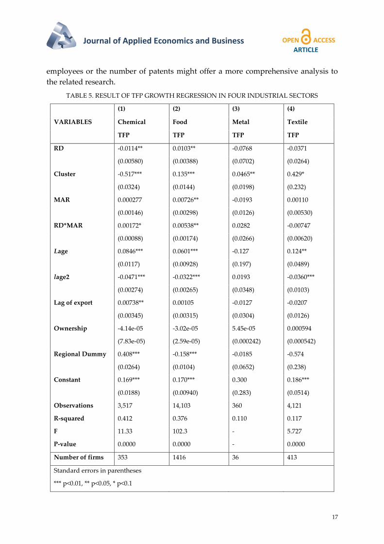
Among the four sectors, the significant coefficient of RD only occurs in the chemical
and the food sectors, as shown in the Table 5. In the food sector, firms that conduct
R&D activity in a competitive location significantly have higher TFP growth than

Femi Sukmaretiana The Role of R&D and Location in a Cluster on
Total Factor Productivity Growth of Indonesian Manufacturing
16 JOURNAL OF APPLIED ECONOMICS AND BUSINESS, VOL. 4, ISSUE 4 - DECEMBER, 2016, PP. 5-20
firms without R&D activity. Meanwhile, in the chemical sector, the significant
coefficient of RD and RD*MAR indicates that firms in the competitive location with
R&D activity have lower TFP growth than firms without R&D activity. The
insignificant coefficient of RD in the metal and the textile sectors indicate that there
is no difference of total factor productivity growth between firms with R&D activity
and without R&D activity in both sectors. Even though the firms with R&D activities
in the chemical sectors have less TFP growth compared with firms without the R&D
activities and for the other sectors the firms with and without R&D activity shows no
different in the TFP growth, it doesn’t mean that the R&D activity has negative or no
effect on the TFP growth of the firms. If the information about the performance of
R&D activity of firms is available, we could further examine the impact of firms’
R&D activity on their TFP performance.
The effect of cluster shows positive, significant results for TFP growth in the food,
metal and textile sector. This means that firms located in a cluster get higher TFP
growth in those three sectors. This result in line with the argument by Porter (1998)
who states that being in a cluster will benefit the firms and increase their
productivity. While for the chemical sector, the negative sign of cluster shows that
firms located in a cluster get lower TFP growth compared with firms that not located
in the cluster. Firms that located in the industrial cluster can also have the negative
effect of congestion that cause the increasing in the cost of production such as
excessive pollution, and higher infrastructure cost because of the emergence of new
firms in cluster area (Press, 2006: 54). The negative sign in this result indicates the
congestion effect of cluster that gives negative effect on a firm’s productivity in the
cluster.
The estimation results on the age variable show that as the firms get older, they are
becoming more productive (in the food, chemical and textile sectors). However,
when they reach a certain age, their productivity will decline. This finding indicates
that the learning process and accumulation of experience through time tend to
promote TFP Growth. The export dummy variable is statistically significant and has
a positive effect on the productivity only on chemical sector. This finding indicates
that firms in that sector that conduct an export activity tend to achieve a higher
growth in total factor productivity. This result confirms Greenaway and Keller (2007)
study that a firm can get “learning effect” from the export activity and imply their
improvement in productivity. Meanwhile, the regional dummy variable shows the
various result for the four sectors.
Finally, this study recommends some insights for the future research. In this study,
only a dummy variable for R&D activity was employed. However, a more precise
result might be obtained when using research expenditure as the proxy of R&D
activity. In addition, a study that includes other information related to R&D
activities such as the number of R&D employees, the level of education of the R&D
Journal of Applied Economics and Business
17
employees or the number of patents might offer a more comprehensive analysis to
the related research.
TABLE 5. RESULT OF TFP GROWTH REGRESSION IN FOUR INDUSTRIAL SECTORS
VARIABLES
(1) (2) (3) (4)
Chemical Food Metal Textile
TFP TFP TFP TFP
RD -0.0114** 0.0103** -0.0768 -0.0371
(0.00580) (0.00388) (0.0702) (0.0264)
Cluster -0.517*** 0.135*** 0.0465** 0.429*
(0.0324) (0.0144) (0.0198) (0.232)
MAR 0.000277 0.00726** -0.0193 0.00110
(0.00146) (0.00298) (0.0126) (0.00530)
RD*MAR 0.00172* 0.00538** 0.0282 -0.00747
(0.00088) (0.00174) (0.0266) (0.00620)
Lage 0.0846*** 0.0601*** -0.127 0.124**
(0.0117) (0.00928) (0.197) (0.0489)
lage2 -0.0471*** -0.0322*** 0.0193 -0.0360***
(0.00274) (0.00265) (0.0348) (0.0103)
Lag of export 0.00738** 0.00105 -0.0127 -0.0207
(0.00345) (0.00315) (0.0304) (0.0126)
Ownership -4.14e-05 -3.02e-05 5.45e-05 0.000594
(7.83e-05) (2.59e-05) (0.000242) (0.000542)
Regional Dummy 0.408*** -0.158*** -0.0185 -0.574
(0.0264) (0.0104) (0.0652) (0.238)
Constant 0.169*** 0.170*** 0.300 0.186***
(0.0188) (0.00940) (0.283) (0.0514)
Observations 3,517 14,103 360 4,121
R-squared 0.412 0.376 0.110 0.117
F 11.33 102.3 - 5.727
P-value 0.0000 0.0000 - 0.0000
Number of firms 353 1416 36 413
Standard errors in parentheses
*** p<0.01, ** p<0.05, * p<0.1

Femi Sukmaretiana The Role of R&D and Location in a Cluster on
Total Factor Productivity Growth of Indonesian Manufacturing
18 JOURNAL OF APPLIED ECONOMICS AND BUSINESS, VOL. 4, ISSUE 4 - DECEMBER, 2016, PP. 5-20
CONCLUSION
This study examine the role of R&D activity and firms’ location in an industrial
cluster to the total factor productivity growth for manufacturing sector in Indonesia
using a balanced panel data in four sectors of manufacturing (chemical, food, textile
and metal). Stochastic frontier analysis is employed to estimate the efficiency of
firms and decomposed the total factor productivity growth.
The finding shows that R&D activity significantly affects the TFP growth of firms on
the food and chemical sectors. However, R&D activity does not significantly affect
the metal and textile sectors. These results might be due to the data limitation used
in this study that not capture the performance of the R&D unit of firms specifically.
Additionally, compared to the firms that are not located in cluster, on the food, metal
and textile sectors, the firms that perform their activities in the industrial cluster tend
to gain a higher TFP growth. Nevertheless, on the chemical sector, the firms that are
located in a cluster is found to get lower TFP growth compared to firms outside
industrial cluster, indicating the congestion effect of cluster. These findings conclude
that in general, being in a cluster will benefit the firms to get higher TFP growth.
However the congestion effect also should be considered to avoid the negative effect
of the cluster. The results of this study also show that TFP growth on chemical, metal,
food and textile sector are 5.8%, 3.3%, 7.3% and 6.4% respectively. The technical
progress mainly contributes to the total factor productivity growth.
RECOMMENDATION
The main finding of this study indicates that R&D activity and industrial cluster
positively affect the TFP growth of the firms. Therefore, to stimulate the
improvement of TFP growth, the government should give incentive to encourage the
firms conducting R&D activity and continue the policy of industrial cluster to
stimulate the innovation by taking account the congestion effect of the cluster. In
addition, the quality of labor must always be enhanced to improve the adaptation of
technology.
REFERENCES
Abramovitz, M. (1956). Resource and Output Trends in the United States Since 1870,
National Bureau of Economic Research.
Aswincahyono, H. & Hill, H. (2002). 'Perspiration' versus 'Inspiration' in Asian
Industrialisation: Indonesia before the Crisis, Journal of Development Studies, 38(3),
138-163.
Berry, A., Rodriguez, E. & Sandee, H. (1999). Firm and group dynamics in the role of
the SME sector in Indonesia, Paper presented to the World Bank project on role of
small and medium enterprises in development.
Journal of Applied Economics and Business
19
Cohen, W. & Levinthal, D. (1989). Innovation and learning: The two face of R&D,
The Economic Journal, 99(397), 569-596.
Farrel, M. J. (1957). The Measurement of Productive Efficiency, Journal of Royal
Statistical Society Series A, 120, 253-290.
Greenaway, D. & Kneller, R. (2007). Firm heterogeneity, exporting and foreign direct
investment, Economic Journal, 117, 134-161.
Griffith, R., Redding, S. & Van Rennen, J. (2004). Mapping the two face of R&D:
Productivity growth in in a panel of OECD industries, Review of Economics and
Statistics, 86(4), 883-895.
Ikhsan, M. (2007). Total Factor Productivity Growth in Indonesian Manufacturing: A
Stochastic Frontier Approach, Global Economic Review: Perspective on East Asian
Economies and Industries, 36(4).
Klenow, P. & Rodriguez-Clare, A. (1997). A neoclasical revival in growth economics:
Has it gone too far? NBER Macroeconomics Annual, 12, 73-103.
Kodde, D. & Palm, F. (1986). Wald Criteria for Jointly Testing Equality and
Inequality Restrictions, Econometrica 54(5), 1243-1248.
Kumbhakar, S. & CAK, L. (2000). Stochastic Frontier Analysis. NY, USA: Cambridge
University Press.
Margono, H. & Sharma, S. (2006). Efficiency and Productivity Analyses of
Indonesian Manufacturing Industries, Journal of Asian Economics, 17, 979-995.
Ministry of Industry. (2012). Industry Facts and Figures, Jakarta: Public
Communication Centre.
Najib, M., Kiminami, A. & Yagi, H. (2011). Competitiveness of Indonesian Small and
Medium Food Processing Industry: Does The Location Matter?, International Journal
Of Bussiness and Management, 6(9), 57-67.
Porter, M. E. (1998). Cluster and New Economics of Competition, Harvard Bussiness
Review, 80.
Press, K. (2006). A Life Cycle for Clusters?: The Dynamics of Agglomeration,
Change, and Adaption, New York: Physica-Verlag Heidelberg.
Romer, P. (1990). Endogenous technological change, Journal Politic and Economic,
98, 71-102.
Solow, R. M. (1957). Technical Change and the Aggregate Production Function,
Review of Economics and Statistics, 39(3), 312-320.
Femi Sukmaretiana The Role of R&D and Location in a Cluster on
Total Factor Productivity Growth of Indonesian Manufacturing
20 JOURNAL OF APPLIED ECONOMICS AND BUSINESS, VOL. 4, ISSUE 4 - DECEMBER, 2016, PP. 5-20
Suyanto, S. R. & Bloch, H. (2009). Does foreign direct investment lead to productivity
spilllovers? Firm level evidence from Indonesia, World Development, 37(12), 1861-
1876.
Tijaja, J. & Faisal, M. (2014). Industrial Policy in Indonesia: A Global Value Chain
Perspective. ADB Economics Working Paper Series, 15.
Timmer, M. (1999). Indonesia's Ascent on the Technology Ladder: Capital Stock and
Total Factor Productivity in Indonesian Manufacturing, 1975-1995, Bulletin of
Indonesian Economic Studies, 35(1), 75-97.
Zahra, S. & George, G. (2002). Absortive capacity: a review, reconceptualization and
extension, Academy of Management Review, 27, 185-203.
World Bank (May 2016) Wholesale Price Index. http://data.worldbank.org/indicator/
FP.WPI.TOTL?locations=ID (Accessed the 20th of May 2016).

Journal of Applied Economics and Business
21
FUTURE SCENARIOS AND EFFICIENT
TRANSPORTATION 2030 – DB
SCHENKER
Monika Trpevska
MsC. Student, “Goce Delcev” University - Stip, Faculty of Tourism and Business Logistics, Macedonia
Abstract
This paper refers to a vision of the future in terms of logistics and transportation provided and developed by the
team from the worldwide company of German origin, DB Schenker. This company is among the best in the area,
not just the perfect function in over 2,000 locations around the world and actually works with great success, but
recently released and presented his plan or vision for the future scenarios in terms of transport and logistics
Germany. First growth of logistics in Germany is shown as a percentage, and then through pictures and urban
planning are shown visions or future scenarios to be completed by 2030. In this study is used the method of
research for both current and previous logistic situations in Germany, and the vision for 2030 determined by
inquiries of employees, experts at DB Schenker and under agreements with the Government of Germany.
Key words
Transport, Predictions, Environment, Logistic management
INTRODUCTION
The demand for freight transportation has been rising for many years at both national
and global level. Existing transport volumes are already overloading today's
infrastructure at difficult-to-expand bottlenecks. At the same time, population shifts
are in evidence, indicating a growing number of people living in cities and
metropolitan regions, while increasing individualization is another factor that will
transform the logistics of tomorrow. These are just some of the trends that will
intensify in thе coming years, leading us to ask: How can Germany cope with
transport volumes up to the year 2030 with its existing infrastructure? To answer this
question, the Fraunhofer Institute for Material Flow and Logistics (IML) has produced
its "Visions of the Future: Transportation and Logistics 2030" study, initiated by
Daimler and DB Schenker. The study highlights the impact and developments
associated with the megatrends that have been identified – globalization,

Monika Trpevska
Future Scenarios and Efficient Transportation 2030 – DB Schenker
22 JOURNAL OF APPLIED ECONOMICS AND BUSINESS, VOL. 4, ISSUE 4 - DECEMBER, 2016, PP. 21-29
demographic change, urbanization, sustainability and resource scarcity – and presents
approaches to solving these. It places these in nine future scenarios that combine the
potential synergies of the individual approaches and identify and describe the
research needed in the years ahead. The scenarios show ways of meeting the
challenges of tomorrow and increasing the efficiency of transportation while
protecting the environment and safeguarding the supply of goods.
Focusing on road and rail transportation in Germany, this paper presents the impacts
and developments that have been identified and divides them into the five
megatrends: globalization, demographic change, urbanization, sustainability and
resource scarcity. Alongside recent studies and publications, it draws upon expert
industry knowledge taken from interviews and discussions. Also there are previous
researches from the work of DB Schenker by a highly professional team, and the
results of previous plans and forecasts.
LITERATURE REVIEW
Main culprits or responsible for starting this so called project or plan views Logistics
2030 are Prof. Dr. Uwe Clausen, Fraunhofer Institut für Materialfluß und Logistik
(IML) & Institut für Transportlogistik (ITL), Technische Universität Dortmund,
Director, Klaus-Dieter Holloh, Daimler AG, Head of Advanced Engineering, Daimler
Trucks and Michael Kadow, DB Mobility Logistics AG, Vice President Business
Excellence DB Schenker. Setting the foundation for writing these predictions logistics
in 2030, heads of DB Schenker and Daimler are served with the previous work of DB
Schenker, the results of the past, previous planning and realization as well as literature
and facts from other major companies, banks and government of Republic of Germany
as well as many others, like: Acatech (2010), BMVBS Federal Ministry of Transport,
Building and Housing (2011), BP Statistical Review of World Energy (2013), Bpb -
German Federal Agency for Civic Education (2009), Bundesregierung (German
Federal Government) (2009), Daimler Trucks (2012), Deutsche Post AG (2009), DVWG
(German Association of Transport Sciences) (2009), Frankfurter Allgemeine Zeitung
(2012), Holtbrügge & Welge (2010), Institute for Mobility Research (2005), Pfohl &
Flickinger (1998), ProgTrans AG (2007), DB Schenker (2012), Schmidt & Kille (2008),
Wietschel (2008) and the World Bank (2014).
FUTURE SCENARIOS 2030
Nine future scenarios are developed for road and rail freight transportation in the
context of innovative and sustainable transport systems. These build on the trends
and innovations already identified.

Journal of Applied Economics and Business
23
Integrating systems to enable goods in transit to be monitored and managed in
real time
Increasing digitization and networking of objects provides the basis for the Internet of
Things (cyber-physical systems). This gives rise to intelligent load carriers, which
provide transport information for immediate processing. The rapid provision of
information and communication between the load carriers themselves creates self-
controlling and flexible transportation chains. The freight makes real-time decisions,
based on real data and events, on the route it will take though the transportation
network. It is possible to change the route or mode of transport at short notice and
optimize transportation chains in terms of capacity utilization, transport time,
environmental factors and costs. There is therefore more focus on the integration of
different modes of transport and decentralized decision making in real time when it
comes to scheduling and shipping. Managing the Internet of Things and combing it
with intelligent traffic guidance systems makes better use of existing infrastructure
capacity. For example, longer routes increase the transport volume but also save time
and improve reliability. This has an impact on the internal processes of transportation
and transshipment companies. The rapid provision of electronic information
streamlines processes and eliminates the need for time-consuming data collection
upon the cargo's arrival at its destination. A further advantage is the optimized
planning and utilization of resources enabled by the preannounced arrival times.
Vehicle-to-vehicle communication is extensively introduced. Transmitting data on
status and surroundings means danger can be reduced or avoided as vehicle
electronics intervene directly or warn the human driver. The Internet of Things helps
to bring about new services based on the automated control of load carriers by the
transportation network.
Using infrastructure efficiently with intelligent traffic guidance systems
In future, all road users' vehicles are equipped with ever more modern navigation
devices. This enables extensive data to be transferred and offers new options to assist
navigation. Infrastructure, too, becomes ever more closely integrated with such
intelligent guidance systems. The integration of different modes of transport and
infrastructure provides real-time data to guide road users. Freight traffic is clearly
distinguished from private transport so that individualized traffic forecasts for
different road users become a reality. To avoid traffic congestion, alternative routing
shows each road user the most resource-efficient and quickest way to their destination
and is customized to their individual needs. A precise forecast or arrival time can be
given, enabling more efficient route planning in freight transportation. The route
calculation not only includes major roads and highways, but also smaller roads. It

Monika Trpevska
Future Scenarios and Efficient Transportation 2030 – DB Schenker
24 JOURNAL OF APPLIED ECONOMICS AND BUSINESS, VOL. 4, ISSUE 4 - DECEMBER, 2016, PP. 21-29
additionally takes into account environmental zones, preferred routes for trucks and
road closures.
Individualized routing, customized to the type of vehicle and with networked
assistance systems, therefore means more resource-efficient transportation on roads
and rails alike. To make this system work, vehicles must be equipped over the coming
years with the technologies needed to continuously transmit and receive real-time
data.
Safe and efficient transportation with driver assistance systems
Greater communication and networking between road users in future is achieved by
equipping growing numbers of vehicles with modern technologies. This increases the
number of information sources that can be used to create a safe and efficient flow of
traffic. Radar, infrared and video cameras on modern vehicle fleets, for example,
enable additional information and hazards to be detected and identified. Networked
assistance systems can use this data and inform the driver visually or acoustically.
This takes the burden off drivers by supporting them in their work environment.
Depending on the extent to which these technologies are applied in future, they take
the form of individual driver aids to assist, for example, in maintaining a safe distance,
keeping in lane and driving at night, or are developed and combined to make the leap
from driver assistance to autonomous driving. Truck convoys are one possible use for
this technology. The trucks drive themselves in a line at equal distance from one
another, all controlled by a driver in the truck at the front of the convoy. The remaining
trucks are accompanied by trained staff able to intervene in an emergency. In the
shorter term, these autonomous technologies are used for internal transportation on
self-enclosed factory sites, greatly facilitating processes on the ground. Combining
autonomous vehicles with the integration of systems, i.e. using the Internet of Things
– enables goods or products to be transported autonomously around the factory from
one stage of the process chain to the next. Combing different approaches thus
generates further potential synergy effects, improving the safety and efficiency of
transportation.
Optimizing processes with intelligent freight cars
Intelligent freight cars are complemented by technological innovations such as
automatic couplers and electro-pneumatic brakes. This leads to shorter process times
in forming and dividing trains, reduced braking distance and faster response times by
the train. The result is more effective use of tracks and improved safety thanks to
advanced technology. Synergy effects exist here, for example with intelligent traffic
guidance systems and integration of different modes of transport. The freight cars are
able to decide their own transport route depending on the information provided. This
direct communication simplifies processes and saves valuable resources in future.

Journal of Applied Economics and Business
25
Low noise levels in city logistics with alternative propulsion and new
logistics concepts
Quiet nighttime transport in city logistics still offers major potential to take the strain
off infrastructure as re-urbanization takes its course. If deliveries are to become so
quiet that they can be moved to the nighttime, however, there is still a great deal of
research work to be done, particularly in vehicle and propulsion technologies.
Batteries must be made powerful enough to drive larger trucks or cover greater
distances without needing a recharge.
Using capacity efficiently with modular container design for small transport
volumes
To take the pressure off city centers, the modular containers are combined at
intercompany handover points on the edges of urban areas, forming large loading
units for the line haul, or prepared for delivery. Importantly, this requires an
international standard for the containers to enable the principle to work across
different companies and the different smaller loading units to be packed together
efficiently into larger ones. This cooperative consolidation of transport volumes is
used in future to provide appealing, individualized and efficient transportation
services in CT networks.
Consolidating transport volumes with multimodal integration of different
modes of transport
The integration of different modes of transport is complemented by the use of
innovative, high-speed cargo handling technologies. Together with optimized
interfaces, designing individualized and attractive CT networks enables improved
capacity utilization across all transportation modes and companies. Harmful
emissions of pollution and exposure to it, for example noise caused by city traffic, is
reduced as a result. There is enormous potential to reduce costs at economic level
through efficient resource use.
Modern work environments to make the logistics industry more appealing
Networked assistance systems and modern vehicle fleets support staff at their
workplaces and ease the pressure on them. Such technology also makes it easier for
people to join the industry, including those moving from other careers. Ergonomic
and attractively designed workplaces, such as truck and train cabs, are another factor.
Improving the industry's attractiveness and long-term training provision for skilled
employees strengthens logistics and does not come at the expense of people's own
private and professional goals.

Monika Trpevska
Future Scenarios and Efficient Transportation 2030 – DB Schenker
26 JOURNAL OF APPLIED ECONOMICS AND BUSINESS, VOL. 4, ISSUE 4 - DECEMBER, 2016, PP. 21-29
More environmentally friendly transportation with alternative vehicle and
propulsion technologies
Society's call for "green logistics" demands more environmentally friendly
transportation in future. This is provided by modern vehicle fleets used in a way that
optimizes energy use and carbon emissions. It involves developing both vehicle
technologies, such as better aerodynamics to reduce CO2, and propulsion
technologies. There is unused potential, not only in electric and natural gas
propulsion, but also in existing combustion engine technology, which can be
converted into further CO2 savings through changes to vehicle technologies. Trucks
and locomotives can achieve additional energy efficiency in future with waste heat
utilization. This greater engine efficiency cuts fuel consumption and thus conserves
resources. In future, transportation concepts achieve considerable CO2 efficiency
using optimized vehicle and propulsion technologies that are adapted to the situation.
Modern vehicle fleets therefore save resources and make greater use of
environmentally friendly energy sources. Combining adaptable, individualized route
planning with intelligent traffic control systems enables further resource savings.
EFFICIENT TRANSPORTATION 2030
Germany is one of the world's most important logistics centers. This is thanks both to
its location at the heart of Europe and its well-developed infrastructure. Figure 1
shows the geographical locations of Europe's largest logistics regions and illustrates
their importance.
FIGURE 1. EUROPEAN LOGISTICS REGIONS
Source: Fraunhofer IML | Daimler AG | DB Mobility Logistics AG

Journal of Applied Economics and Business
27
The interaction of the nine future scenarios creates the overall picture of efficient
transportation. The increase in digitization, in information flows before and during
transport, and the ongoing development of vehicle and propulsion technologies,
combined with networked assistance systems, are the prerequisites for efficient
transportation and competitive industries in Germany in the year 2030. Optimizing
the interaction between these individual visions enables further potential for
improving efficiency to be leveraged. For example, technical improvements like
intelligent freight cars support solutions of a more organizational nature – e.g.
consolidation of transport volumes through multimodal integration of carriers. The
Figure 2 shows this development in freight transport for Germany.
FIGURE 2: FORECAST OF VOLUME SOLD IN FREIGHT TRANSPORTATION,
GERMANY UP TO THE YEAR 2050
Source: ProgTrans (2012: 94)
AREAS FOR ACTION
The future scenarios described here for achieving the objectives set and minimizing
the impacts point to various areas for action that will help us to realize the vision of
efficient transportation in the year 2030. The solutions present individual measures
that, despite being full of potential, can only achieve the impact described in the future
scenarios if they are combined with one another.

Monika Trpevska
Future Scenarios and Efficient Transportation 2030 – DB Schenker
28 JOURNAL OF APPLIED ECONOMICS AND BUSINESS, VOL. 4, ISSUE 4 - DECEMBER, 2016, PP. 21-29
Like the individual solutions, the areas for action are categorized into the three areas
of innovation: digitization, technology and flexible management. While digitization
enables optimized planning based on real-time data, improving technology leads to
optimized, energy-efficient and safe processes. Flexible management supports
collaboration within and between companies. The areas for action identified are also
grouped into four types of transportation: cross-carrier, rail freight, and local and
long-distance road traffic. Figure 3 summarizes the areas for action in a matrix.
Cross-carrier Rail freight Road (regional
traffic)
Road (long-
distance-traffic)
Digitization Internet of Things
(syber physical
systems)
Intelligent freight
cars
Internet of Things
(syber physical
systems)
Intelligent traffic
guidance systems
Internet of Things
(syber physical
systems)
Intelligent traffic
guidance systems
Internet of Things
(syber physical
systems)
Flexible
management
Deceleration
Cooperative
consolidation of
transport
volumes
CT networks
Integrating mode
of transport
Attractive
workplace design
Cooperative
consolidation of
transport
volumes
Quiet nighttime
transport
Cooperative
consolidation of
transport
volumes
Attractive
workplace design
Cooperative
consolidation of
transport
volumes
Technology CT Networks
Modular
container design
Waste heat
utilization
Automatic
coupling
Autonoumos
driving
Hybrid
locomotive
Vehicle and
propulsion
technologies
Autonoumos
driving
Modern vehicle
fleets
Waste heat
utilization
Networked
assistence
systems
Vehicle and
propulsion
technologies
Autonumos
driving
Modern vehicle
fleets
Waste energy
utilization
Networked
assistence
systems
FIGURE 3. MATRIX - SUMMARIZED AREAS FOR ACTIONS
CONCLUSION AND RECOMMENDATIONS
The future scenario we describe aims to achieve the objectives set and minimize
impacts. It shows various areas for action that have been identified for efficient
transportation in the year 2030. We categorize these into the three areas of innovation:
digitization, technology and flexible management.
While digitization enables optimized planning based on real-time data, improving
technology leads to optimized, energy-efficient and safe processes. Flexible

Journal of Applied Economics and Business
29
management supports collaboration within and between companies. These areas for
action and their potential synergies give rise to the vision of efficient transportation in
the year 2030.
With a focus on road and rail freight, scenarios are examined and developed for the
future based on innovative and sustainable transportation systems in the context of
growing transport volumes. Those scenarios require no more than minor changes to
infrastructure. As well as identifying global trends, influential factors and effects on
the efficiency of transportation, various solutions are described as capable of tackling
future challenges and fulfilling the target requirements set.
REFERENCES
Acatech – German Academy of Science and Engineering. (2010). Mobilität 2020. Perspektiven
für den Verkehr von morgen, 35-36.
BMVBS Federal Ministry of Transport, Building and Housing, (2011). Bundesministerium für
Verkehr, Bau und Stadtentwicklung: Lkw-Parken in einem modernen, bedarfsgerechten
Rastanlagensystem.
BP. (2013). Statistical Review of World Energy, 12-13.
Bpb - German Federal Agency for Civic Education. (2009). Bundeszentrale für Politische
Bildung: Zahlen und Fakten Globalisierung.
Bundesregierung (German Federal Government). (2009). Nationaler Entwicklungsplan
Elektromobilität der Bundesregierung.
Daimler Trucks. (2012). Alternative Kraftstoffe: Econic LNG setzt die Reichweite auf neues
Niveau.
Deutsche Post AG. (2009). Delivering Tomorrow. Kundenerwartungen im Jahr 2020 und
darüber hinaus, Eine globale Delphistudie, 69-71.
DVWG (German Association of Transport Sciences) (2009). Der Verkehr im Jahr 2030.
Ergebnisse des internationalen Workshops und Kongresses "Traffic and Transport 2030".
Frankfurter Allgemeine Zeitung (2012) Neues Verkehrskonzept. Lastwagen an der
Oberleitung.
Holtbrügge, D. & Welge, M. (2010). Internationales Management: Theorien, Funktionen,
Fallstudien, Wiesbaden: Schäffer-Poeschel Verlag.
Institute for Mobility Research- Institut für Mobilitätsforschung (2005). Zukunft der
Mobilität. Szenarien für das Jahr 2025.

Journal of Applied Economics and Business
30
TOURISM DEMAND IN THE SOUTH-
WEST PLANNING REGION OF
MACEDONIA
Elena Kosturanova
Msc student, Faculty of Computer Science, Goce Delcev University - Stip, Macedonia
Abstract
The paper makes an attempt to forecast tourism demand in the South-west Planning Region (SWPR) of
Macedonia. The author applies the trend analysis model and the simple linear regression model for that purpose.
The linear regression model gave better and more accurate results. According to the ten-year-forecasts obtained
from the linear regression results, it is expected an insignificant increase of tourism demand in the SWPR. Yet,
according to the ten-year forecasts obtained from the trend analysis model, it is expected a great increase of tourism
demand in this region. It should always have in mind that the forecasts can never be absolute accurate due to
many influential factors. Regardless the applied method, it cannot explain the changes and reasons behind that.
Key words
Forecasting, Tourism demand, South-west Planning Region, Macedonia
INTRODUCTION
Tourism today is a global industry involving hundreds of millions of people in the
international and domestic trips each year. The World Tourism Organization (WTO)
estimated that in 2015 there were 1.184 million international travellers although some
of this activity consists of the same travellers involved in more than one trip per year
and the precise scale of the tourism industry is in doubt.
Tens of millions of people globally work directly in the industry and many more are
employed indirectly. Hundreds of millions of people receive income from tourist
activities because they live in so-called destination areas as "homely" population.
Millions of dollars are spent each year to advertise and promote vacations and travel
products. For much of recorded history, the journey was difficult, inconvenient,
expensive, and often dangerous. However, journeys were undertaken and it suggests
some strong motivating factors. In the last 150 years, travel has become more

Journal of Applied Economics and Business
31
affordable and not so hard, so that those who travel were prepared to admit that the
pleasure was one of the motivations for their trip.
20 years ago, the key objectives of tourism planning were summarized as follows: "to
ensure that visitors have a chance to gain a satisfactory and pleasurable experience
and at the same time to provide funds to improve the lives of residents and areas of
destination." Williams (Mason, 2016) suggested a number of overall objectives for
tourism planning. He pointed out that can help to shape and control schemes for
development, to save limited resources and provide a framework for active promotion
and marketing destinations and can be a mechanism for integrating tourism with
other sectors. He proposed a number of key objectives in tourism planning:
o Create a mechanism for structured commission for tourist facilities within the
very large geographical areas;
o Coordination of the fragmented nature of tourism (especially in terms of
accommodation, transport, marketing and human resources);
o Specific interventions to save resources and increase the benefits for the local
community in an effort to achieve sustainability (usually through tourism
development or management plan); and
o Distribution of tourism benefits (development of new tourism sites or economic
regroupings of places that tourists began to leave).
The paper is structured in several parts. After the introductory section, it proceeds
with a section that briefly describes tourism demand and explains the term ‘tourism
demand’. The third section is a background material on forecasting, which describes
the phases of forecasting. After that, there is section with some basic information on
the South-west Planning Region. The paper proceeds with explanation of
methodology, while the final part is the conclusion.
TOURISM DEMAND
Tourism demand is a broad term that encompasses the factors that regulate the level
of demand, the spatial characteristics of the demand, various types of demand and the
reasons for making such requests. Cooper et al, (1998) define the demand as a
"schedule of the amount of any product or service that people want and are willing to
buy of each specific price in a set of possible prices during a period of time”.
Individuals known as tourists generate tourism demand. This happens to a certain
place called "tourist destination". The scope and magnitude of demand vary over time,
and sometimes with the seasons. Time demand for tourist services either promotes or
changes. Such changes may be due to the emergence of so-called "new tourists" who

Elena Kosturanova
Tourism Demand in the South-west Planning Region of Macedonia
32 JOURNAL OF APPLIED ECONOMICS AND BUSINESS, VOL. 4, ISSUE 4 - DECEMBER, 2016, PP. 30-42
want to experience something new and expect high quality services and value for their
money. New tourists carry different levels of demand.
There are three main types of demand: the real, hidden and latent demand. The real
demand which is also called effective demand comes from tourists who are involved
in the actual process of tourism. The second type of demand is the so-called repressed
demand created by two categories of people who are usually able to travel due to
circumstances beyond their control. The first group includes those sections of the
population who would like to be involved in tourism, but for one reason or another
cannot. Because they can participate at a later date, this situation is called potential
demand. Delayed demand describes the second subcategory of suppressed demand
that the trip was postponed due to problems of supply in the environment. The third
type is latent demand. It refers to the spatial and temporal expression of the demand
of a particular country, for example, demand for tourist accommodations or travel
service to a particular destination. Tourism demand can be defined in different ways
depending on the economic, political, psychological and geographical point of view
of the author (Petrevska, 2014).
The size of demand for travel to a particular destination is very important for everyone
involved in tourism. The vital data on demand include: (1) How many visitors arrived;
(2) Means of transport; (3) Duration of stay and type of accommodation; and (4)
Money spent. There are various measures of demand, some are very easy to obtain
and are usually of a more general interest than others. There are also techniques for
predicting the demand. Such estimates are of great interest to anyone involved in
planning tourism development. More precisely, the demand for travel to a particular
destination may be a function of the propensity of a person to travel and the resistance
to travel.
𝐷 = 𝑓(𝑝𝑟𝑜𝑝𝑒𝑛𝑠𝑖𝑡𝑦, 𝑟𝑒𝑠𝑖𝑠𝑡𝑎𝑛𝑐𝑒) (1)
In equation (1) there are two arguments: the tendency that depends on the
psychological profile, socio-economic status and resistance to marketing and travel-
dependent economic distance, cultural distance, the cost of tourism services, service
quality and seasonality. Propensity can be considered as a predisposition of a person
to travel, in other words, if the person is ready to travel, what types of trips he/she
wants, and what types of destinations are considered. Propensity of a person to travel,
obviously, may be determined largely by its psychographic profile and motivation for
the trip. In addition, the socio-economic status may have an important impact on the
propensity to travel. It follows that to estimate the propensity for traveling, we must
first understand the psychographic and demographic variables related to the
personality. Propensity is directly linked to the demand. On the other hand, the
resistance refers to the relative attractiveness of different destinations. This factor is a
function of several variables, such as economic distance, cultural distance, the cost of
tourist services in the destination, quality of service of destination, the effectiveness of
Journal of Applied Economics and Business
33
advertising and promotion and the season. Hence, the resistance is inversely related
to demand.
The economic distance refers to the time and cost involved in traveling from the origin
to the area of destination and back. The higher economic distance, the greater the
resistance to that destination and consequently reduced demand. One may conclude
that between any origin and destination point, if travel time or travel expenses can be
reduced, demand will increase.
The cultural distance refers to the extent in which the culture of the region of origin of
the tourist is different from the culture of the host region. In general, the greater the
cultural distance,the greater the resistance is. The greater cost of tourist services, the
greater the resistance to travel to the destination is and therefore we will have a
reduction of tourist demand. This variable captures the famous inverse relationship
between the price of a product or service and the demand for it (Goeldner and Ritchie,
2003).
The higher the quality of services is, there will be less resistance to travel to the
destination. Although the relationship between quality of service and demand is clear
enough, difficulties emerge in the interpretation and evaluation of quality. The
assessment of quality is a very personal thing, and the quality for one tourist does not
mean quality for another. Second, if the tourist has no previous experience with the
travel destination, how can he accurately judge the quality of services there? In this
case, the tourist should choose a destination based on the quality of service. Very often
for the wrong ads or inaccurate information from the other, the perception of quality
of tourist services cannot be reached within the destination. This situation has serious
implications for establishing repeat customers, which is an important ingredient for
success in tourism business. As a result, the destination must be accurate in projecting
the correct image.
The effect of seasonality of demand is quite obvious. The relative attractiveness of a
particular destination will depend on the time of year that the holiday is planned. For
ski resort, for example, demand will be the highest during the winter months, while
the resistance is the least at this season.
BACKGROUND MATERIAL ON FORECASTING
Scientific approach to tourism planning involves forecasting tourism demand as a
starting point in the planning process. The forecast warns of useful actions to be taken
to achieve the objectives. Success depends primarily on the accuracy of predictions.
Although it is almost impossible to conduct accurate forecasting of tourism demand,
it will greatly affect the reduction of uncertainty about the movements of a particular
phenomenon or event in the future.

Elena Kosturanova
Tourism Demand in the South-west Planning Region of Macedonia
34 JOURNAL OF APPLIED ECONOMICS AND BUSINESS, VOL. 4, ISSUE 4 - DECEMBER, 2016, PP. 30-42
Given that demand is not stable on tourism market, well performed prediction is a
key prerequisite for success. The tourism demand is characterized by large seasonal
fluctuations that typically occur as a consequence of the change of season during the
year, which is very notable in tourist destinations offering sun and beach. However,
there are other factors that may cause cycles in tourist movements, such as school
holidays, vacations, or special events in the tourist destination (festivals, exhibitions,
sporting events, etc.). At the same time, the movement of tourist demand may affect
both unpredictable and irregular elements, such as sudden changes in prices,
epidemics, floods, war, etc. Therefore, when forecasting tourism demand, we must
know the main methods of prediction and the advantages and disadvantages of each
selected model.
Forecasting is the process of organizing the past data order to predict its future. Hence,
the prediction process is created to predict future events. Moreover, when it comes to
tourism demand as an event can be considered: the number of tourists in a particular
tourist destination; number of overnight stays in a hotel or group of hotels; number of
passengers traveling from one tourist spot; the number of tourist brochures
distributed to potential tourists, etc. Each item, which is subject to prediction has two
characteristics: the time dimension, and the result. This result shows the exact size of
the demand. However, it may occur qualitative results, and then the predicted next
year tourism demand will be higher, lower or the same than the previous.
The process of forecasting tourism demand consists of the following four main phases:
(1) Preparation phase; (2) Phase of specification i.e. detailed description; (3)
Implementation phase; and (4) Evaluation. They are aimed at establishing a system
that is used continuously for prediction (Frechtling, 1996).
Phase 1. In the preparation phase, the planner chooses the appropriate method for
prediction i.e. the technique for individual design of future events, and not the model.
Thus, to successfully implement this stage, it is necessary to follow these steps:
o Defining the problem;
o Determining what is needed. Primarily relates to the basic required
information;
o Determining variables that shall be predicted;
o Determining available resources;
o Hypotheses;
o Determining availability of data;
o Listing available methods for prediction;
o Application of preliminary selection criteria; and
o Preliminary selection of method.
Phase 2. The second stage of forecasting tourism demand is the phase of specification,
i.e. detailed description. Here actually it is selected the model for prediction, within
the already defined method. So, after the chosen qualitative or quantitative method, it
Journal of Applied Economics and Business
35
follows the detailed analysis, testing and selection of the most appropriate model for
prediction.
Phase 3. In the implementation phase, the prediction is implemented, documented and
presented. If a quantitative method is used, then the selected model should import
values necessary for calculations. If qualitative method is used, then the prediction is
developed based on the responses received from experts involved. Next, if necessary,
an adjustment is performed in the line of correction of the results. The next step is
documenting the applied model. That means in a form of a written report to describe
all previously implemented stages, which models have been tested, rejected and the
reasons for that, and the need to correct the results if that was the case. Only then the
results of the forecasting process can be presented.
Phase 4. Evaluation is the final phase. It begins by testing the accuracy of the forecasts.
That actually means monitoring the ratio between the actual and predicted values.
Thus, the evaluation can be measured by various commonly applied indicators, as:
the Mean Absolute Error (MAE), the Mean Absolute Percentage Error (MAPE), the
Root Mean Squared Error (RMSE), the Theil inequality Coefficient (TIC), etc. If the
assessment shows that there are indeed differences, it is important to determine the
cause (Frechtling, 2012).
The methods for forecasting tourism demand can be divided in two main categories:
quantitative and qualitative. Quantitative methods organize information from the
past phenomenon according to mathematical rules by using basic data patterns. These
methods require objective numerical measurements that are consistent and valid for
a certain historical period. These methods assume that some past patterns will
continue in the future. The data for these methods requires can be obtained from
primary or secondary sources.
There are two main subcategories of quantitative methods: methods of extrapolation
and, the causal methods. The methods of extrapolation are also called methods of time
series analysis and they assume that the movement of the variable in the past will
appear in the future. Patterns in data during the past are used to design or extrapolate
future values. Causal links are ignored. They are often used for tourism demand
forecasting for products for which there is a relatively stable demand, but if they are
not applicable for products with highly variable demand. These methods do not count
the effects of various factors on the movement of tourism demand and still provide
relatively good forecasts. Their results are particularly advantageous when the
prediction is for a shorter period, and at the same time are cheaper than causal
methods. Another subset of quantitative methods is causal methods. They are based
on data from the past movement of tourism demand. Starting from the assumption
that there is a relationship between the forecasting variable and other measurable

Elena Kosturanova
Tourism Demand in the South-west Planning Region of Macedonia
36 JOURNAL OF APPLIED ECONOMICS AND BUSINESS, VOL. 4, ISSUE 4 - DECEMBER, 2016, PP. 30-42
independent variables. The causal methods seek to determine the correct
mathematical expression of this ratio.
The qualitative methods are also called "assessment methods". Previous information
for forecasting variable are organized by experts using their judgment rather than
mathematical rules. They are not necessarily cheaper or easier to implement methods
but have an advantage because they do not require historical data series (Petrevska,
2014).
BACKGROUND MATERIAL ON THE SOUTH-WEST PLANNING REGION
The South-west Planning Region (SWPR) covers the Ohrid Lake and river Treska and
covers an area of 3,340 km2 or 13.4% of the territory of Macedonia. It is one of the eight
planning regions in Macedonia and encompases 13 municipalities: Vevcani,
Vraneshnica, Debar, Debarca, Drugovo, Zajas, Oslomej, Ohrid, Kicevo, Makedosnki
Brod, Plasnica, Struga and Centar Zupa. The basic information on the SWPR is
presented in Table 2.
TABLE 2. BASIC INFORMATION ON THE SWPR, 2011
Number of municipalities 13
Number of populated places 286
Estimation of population 10,83% of total population
Employment rate 27.7%
Unemployment rate 42.4%
GDP per capita 1,807 Euro
Source: State Statistical Office. (2011).
Tourism development is the most distinctive characteristic of the SWPR. This is due
to the fact that it is the most developed region in tourism manner in Macedonia.
Natural features, rich cultural heritage, protected spatial units and long tradition are
the basis for dynamics in tourism. The region has a number of resources at the level
of potential for inclusion in the tourism supply. Also thermal baths are of great
importance for visiting and the development of tourism in this region, while the large
number of churches and historical sites contribute to cultural tourism development.
TABLE 3. TOURISM STATISTICS FOR SWPR, 2014-2015
Item 2014 2015
Total number of tourists 269,547 298,057
Domestic tourists 125,320 136,637
Foreign tourists 144,227 161,420
Total overnights 1,095,452 1,201,927
Overnights of domestic tourists 694,229 745,473
Overnights of foreign tourists 401,223 456,454
Number of rooms 16,304 16,370
Number of beds 42,025 41,917
Source: State Statistical Office. (various years).
Journal of Applied Economics and Business
37
Based on Table 3 one may note in 2015, an increase in the total number of tourists as
well as domestic and foreign, and the number of overnights. It mostly due to the
promotion of Macedonia and Ohrid as a tourist destination, especially in the world
through various advertisements, promotions, exhibitions, videos, programs, etc.
Hence, the foreign tourists are informed and interested in Ohrid, Lake Ohrid and
Macedonia in general, as a country rich with tourist attractions and natural beauties
that are worth to visit. The SWPR has potentials for different types of tourism (Table
4).
TABLE 4. TOURISM POTENTIALS OF THE SWPR
Locality Type of tourism
Ohrid and Lake Ohrid Lake, cultural, fishing, transit, religious, city tourism
Debar Lake, transit, thermal bath tourism
Galicica Mountain, eco-tourism, hunting tourism
Vevcani Rural, cultural tourism
Struga Lake,cultural,fishing,city tourism,transit
Jablanica Mountain,eco-tourism,hunting
Globocica Lake tourism, fishing
Source: (Government of the Republic of Macedonia, 2012)
METHODOLOGY
The main aim of the paper is to predict tourism demand in the SWPR. For that
purpose, two models are applied: the trend analysis model, and the linear regression
model. The main variable is the data on tourist arrivals obtained from the State
Statistical Office. The data set covers the period 2007-2015 (Table 5) for the trend
analysis model, with a projection time 2015-2025. For the linear regression model, the
data set spreads over the period from 2003-2013, with a projection interval 2013-2023.
TABLE 5. TOURIST ARRIVALS IN THE SWPR, 2007-2015
Year Tourist arrivals
2007 255,257
2008 276,669
2009 257,480
2010 234,665
2011 249,746
2012 251,462
2013 264,826
2014 269,547
2015 298,057
Source: State Statistical Office. (various years).

Elena Kosturanova
Tourism Demand in the South-west Planning Region of Macedonia
38 JOURNAL OF APPLIED ECONOMICS AND BUSINESS, VOL. 4, ISSUE 4 - DECEMBER, 2016, PP. 30-42
FIGURE 3. TOURISM DEMAND IN THE SWPR, 2007-2015
Figure 3 visually presents tourists demand for the period 2007-2015. Based on that, the
type of trend is determined that best presents the changes. Whence by continuing the
trend line, we get the forecasted tourism demand by 2025 (Figure 4).
FIGURE 4. FORECASTED TOURISM DEMAND FOR THE SWPR, 2015-2025
On Figure 4 we can see that the trend line is parabolic and for each subsequent year
increases to higher values. If we carefully take a look at the past data (2007-2015), we
may notice that by 2008 there was a growth of tourism demand, followed by a
significant decrease in 2008 and reaching the lowest value of 234,665 arrivals in 2010.
This significant decrease is due to many reasons out of which the most important is
the world economic crisis. The crisis provoked negative impacts in all industries,
including tourism industry, thus provoking drastically decrease in tourism demand.
Then in 2011, a slight increase in noted when tourism demand is getting back on track,
and then it stagnated in 2013, followed by an increase in 2014 and 2015. As reasons for
this drastic increase we can mention the re-commissioning of the airport in Ohrid. This
was followed by many subventions for low-budget flights which resulted in increased
number of passengers, thus boosting development. There was also development of
infrastructure for easier access to tourist resorts. The general promotion of Macedonia
as a tourist destination, also played a major role in increasing tourism demand.

Journal of Applied Economics and Business
39
TABLE 6. FORECASTED TOURISM DEMAND IN THE SWPR, 2016-2025
Year Total tourist arrivals
2016 527,679
2017 577,467
2018 631,321
2019 689,242
2020 751,230
2021 817,284
2022 887,405
2023 961,593
2024 1,039,847
2025 1,122,168
Table 6 presents the forecasted values for tourism demand in the SWPR, in terms of
total tourist arrivals for the period 2016-2025. It is expected the demand continuously
to increase, if the past and current measures that assist tourism development continue.
In 2019, it is expected the total number of tourists that visit the SWPR to reach 689,242
tourists, which is almost additional 100,000 tourists compared to 2015. Up to 2025, it
is expected the demand to reach up to 1,122,168 which, at a first glance looks
overestimated, having in mind that that is the number for Macedonia as a country and
it is very hard to be achieved by the SWPR.
Although estimating extremely positive values, the trend analysis model does not give
any clarification about the figures, but only determines the direction of change. The
second model that was applied for forecasting tourism demand in the SWPR is the
simple (linear) regression model. This model requires to possess data on tourism
demand in recent years as the first variable, and the income per capita (Table 7). The
dependence of the applied variables is graphically presented on Figure 5. The method
of least squares is applied which resulted in a straight line ("best fit") explaining the
inter relation between tourism demand and income per capita (Figure 6).
TABLE 7. TOURIST ARRIVALS AND PER CAPITA INCOME IN THE SWPR, 2003-2013
Year Tourist arrivals Per capita income (MKD)
2003 241,380 86,479
2004 222,950 95,209
2005 236,434 97,861
2006 233,218 106,970
2007 255,257 115,083
2008 276,669 150,771
2009 257,480 140,262
2010 234,665 161,492
2011 249,746 174,509
2012 251,462 170,493
2013 264,826 178,726
Source: State Statistical Office. (different years)
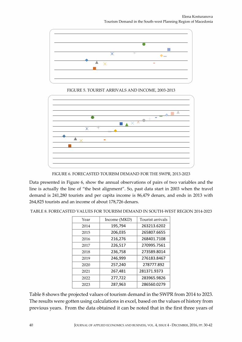
Elena Kosturanova
Tourism Demand in the South-west Planning Region of Macedonia
40 JOURNAL OF APPLIED ECONOMICS AND BUSINESS, VOL. 4, ISSUE 4 - DECEMBER, 2016, PP. 30-42
FIGURE 5. TOURIST ARRIVALS AND INCOME, 2003-2013
FIGURE 6. FORECASTED TOURISM DEMAND FOR THE SWPR, 2013-2023
Data presented in Figure 6, show the annual observations of pairs of two variables and the
line is actually the line of “the best alignment”. So, past data start in 2003 when the travel
demand is 241,280 tourists and per capita income is 86,479 denars, and ends in 2013 with
264,825 tourists and an income of about 178,726 denars.
TABLE 8. FORECASTED VALUES FOR TOURISM DEMAND IN SOUTH-WEST REGION 2014-2023
Year Income (MKD) Tourist arrivals
2014 195,794 263213.6202
2015 206,035 265807.6655
2016 216,276 268401.7108
2017 226,517 270995.7561
2018 236,758 273589.8014
2019 246,999 276183.8467
2020 257,240 278777.892
2021 267,481 281371.9373
2022 277,722 283965.9826
2023 287,963 286560.0279
Table 8 shows the projected values of tourism demand in the SWPR from 2014 to 2023.
The results were gotten using calculations in excel, based on the values of history from
previous years. From the data obtained it can be noted that in the first three years of

Journal of Applied Economics and Business
41
the forecasted period (2014-2017), there are not some significant changes in the
demand, and it ranges between 260,000 to about 290,000 tourists. As of 2018, the
demand starts to grow from 273,589 tourists to 286,560 in 2023. The similar dynamics
may be observed in the income, which starts with 195,794 denars in 2014, and reaches
287,963 denars in 2023. From these results it may be concluded that tourism demand
in the SWPR will grow slightly from year to year and it will move in the same
direction. Some major downs and increases are not expected in the next 10 years,
which means that tourism demand will stagnate. The number of tourists is expected
to grow for around 1% from year to year. The income is also expected to grow for
average 4.5 % which is a significant percentage. From this information can be
concluded that for income growth of 4.5% is expected increase of tourism demand for
about 1% based on the data for previous years (2003-2013).
Taking in consideration that recently Skopje (the capital of Macedonia) has become an
attractive tourist destination, slowly Ohrid (as the leading tourist destination in the
SWPR) is losing the dominant position. Skopje received additional value with the
construction of various monuments, museums and national landmarks, and all that
supported with promotion in foreign countries, contributed Skopje to be more visited
than Ohrid. Tourists whose main destination or only a transit destination is Skopje,
visit the city and various tourist attractions, sites and landmarks there. All these
factors allow us to expect to have reduced tourism demand compared to the past and
on behalf of that we have increased tourism demand. We can expect the future
increase in tourism demand in the region of Skopje. The line of best fit is a straight line
where there are no sharp downs and increases, so we can conclude that tourism
demand as the first variable and income as the second variable has insignificant
increases in their values or stagnate for these reasons. Because disposable income is
significant variable for tourism demand, the simple regression model clarifies
demand. Hence, we conclude that this model has more advantages than other more
sophisticated models, such as multiple regression and computer simulation.
CONCLUSION
Demand is undoubtedly a major measure of success for any region in attracting
visitors. Introduction of methods for measuring or evaluating the current and future
demand, as described in this article, should enable producing accurate data that can
later be used for further research and forecasts. When it comes to tourism demand
forecasting, there are many methods and models that can be applied. However, which
one to use, depends on the available data. Yet, forecasts of tourism demand can never
be 100% accurate because regardless of the model used to process them, they can
always be affected by some external factors that are not in their scope of research so
the method cannot explain the changes and the reasons for that. The South-west

Elena Kosturanova
Tourism Demand in the South-west Planning Region of Macedonia
42 JOURNAL OF APPLIED ECONOMICS AND BUSINESS, VOL. 4, ISSUE 4 - DECEMBER, 2016, PP. 30-42
planning region of Macedonia has the potential to grow into even more attractive
tourism area, if some measures and activities are introduced in the line of supporting
tourism development. The main intention of this article was to portray the current
tourism development in the SWPR, and to present some expectations for the future,
which are satisfactory.
REFERENCES
Centre for development of the South-west planning region. Online data available at
http://www.southwestregion.mk/ZaRegionot.aspx. (Accessed 12 November 2016)
Cooper, C., Fletcher, J., Gilbert, D. & Wanhill, S. (1998). Tourism: Principles and
Practice, London: Longman.
Frechtling, D. (2012). Forecasting tourism demand, Routledge.
Goeldner, C. & Ritchie, B. J. R. (2003). Tourism principles, practices, philosophies, John
Wiley & Sons, Inc. New Jersey.
Government of the Republic of Macedonia. (2012). National strategy for tourism
development 2011-2015, Skopje.
Mason, P. (2016). Tourism Impacts, Planning and Management.
Petrevska, B. (2004). Tourism Planning (in Macedonian), EDNOTERA - Skopje.
State Statistical Office. (various years). Statistical Yearbook, Skopje.
State Statistical Office. (2011). Tourism in the Republic of Macedonia, Skopje.
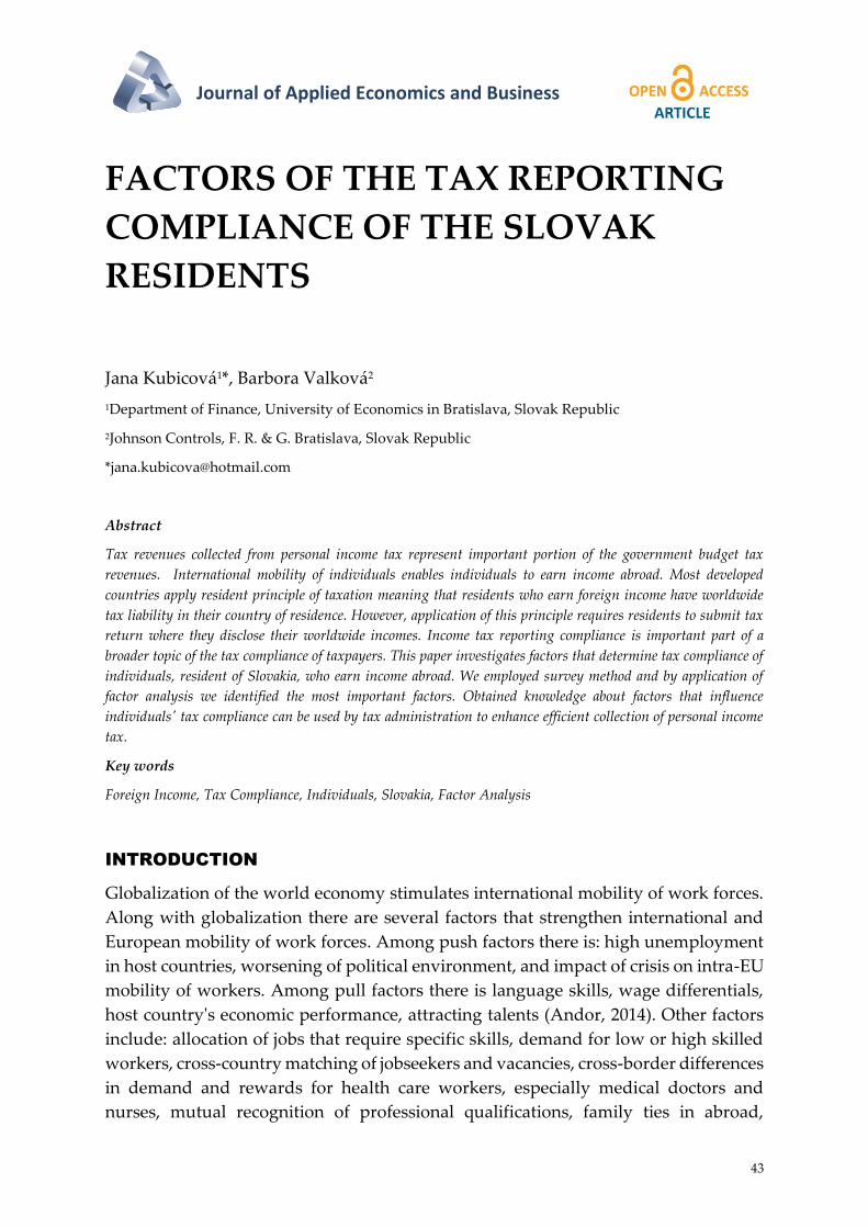
Journal of Applied Economics and Business
43
FACTORS OF THE TAX REPORTING
COMPLIANCE OF THE SLOVAK
RESIDENTS
Jana Kubicová1*, Barbora Valková2
1Department of Finance, University of Economics in Bratislava, Slovak Republic
2Johnson Controls, F. R. & G. Bratislava, Slovak Republic
Abstract
Tax revenues collected from personal income tax represent important portion of the government budget tax
revenues. International mobility of individuals enables individuals to earn income abroad. Most developed
countries apply resident principle of taxation meaning that residents who earn foreign income have worldwide
tax liability in their country of residence. However, application of this principle requires residents to submit tax
return where they disclose their worldwide incomes. Income tax reporting compliance is important part of a
broader topic of the tax compliance of taxpayers. This paper investigates factors that determine tax compliance of
individuals, resident of Slovakia, who earn income abroad. We employed survey method and by application of
factor analysis we identified the most important factors. Obtained knowledge about factors that influence
individuals' tax compliance can be used by tax administration to enhance efficient collection of personal income
tax.
Key words
Foreign Income, Tax Compliance, Individuals, Slovakia, Factor Analysis
INTRODUCTION
Globalization of the world economy stimulates international mobility of work forces.
Along with globalization there are several factors that strengthen international and
European mobility of work forces. Among push factors there is: high unemployment
in host countries, worsening of political environment, and impact of crisis on intra-EU
mobility of workers. Among pull factors there is language skills, wage differentials,
host country's economic performance, attracting talents (Andor, 2014). Other factors
include: allocation of jobs that require specific skills, demand for low or high skilled
workers, cross-country matching of jobseekers and vacancies, cross-border differences
in demand and rewards for health care workers, especially medical doctors and
nurses, mutual recognition of professional qualifications, family ties in abroad,
Jana Kubicová, Barbora Valková
Factors of the Tax Reporting Compliance of the Slovak Residents
44 JOURNAL OF APPLIED ECONOMICS AND BUSINESS, VOL. 4, ISSUE 4 - DECEMBER, 2016, PP. 43-62
occurrence of international marriages, transformation of formerly temporary stay in
host country into to the center of living, shifts of homes motivated by more plausible
weather, adventure, and searching for new experience.
There is one additional important force which intensifies international mobility of
Slovak workforces: fundamental right to free mobility of work forces within the
European Union. Slovak Republic, having been a Member State of the European
Union since May 1, 2004, must follow provisions of the Treaty on the Functioning of
the European Union (TFEU, hereinafter Lisbon Treaty), which has been in effect since
January 1, 2009. Articles 45-48 of Lisbon Treaty laid down freedom of movement of
citizens including workers within the internal market of the European Union.
The right to free movement of workforces has impact on cross-country movement of
workforces. Intra-EU mobility flows declined considerably during the first phase of
the economic crisis – in 2009 and 2010, mobility flows fell by 41% compared with 2007-
2008. In 2011-2012 intra-EU labor mobility increased by 22% compared with 2000-
2010. Some EU countries, among them Greece, Spain, Ireland, Hungary and Latvia
experienced growing labor outflows due to extremely high level of unemployment. It
is estimated that recently more than 1.2 million people work cross-border in the EU.
Gross wages paid to cross-border and seasonal workers in 2010 amounted to €46.9
billion (European Commission, 2012). Worker mobility has been identified as one of
the key potentials for increasing growth and employment in Europe. The importance
of migration in Europe is shown also in the report of the German Destatis, which states
that in January 2011 in the EU there were employed 33,2 million people who were not
nationals of the country in which they work, while more than a third of them (12, 8
million) were citizens of another EU country. According Lászlo Andor, European
Commissioner, in 2013 there were around 7 million EU citizens – or 3,3% of the EU’s
total labor force – working and living in a member country other than their country of
citizenship. In addition, there were 1,1 million cross-border or frontier workers
(Andor, 2014: 4). Eurostat data states that in 2014 there were 15.2 million persons living
and working in an EU Member State of which they were not a citizen, accounting for
7.0% of total EU employment and 7.3 million of them were citizens from another EU
Member State and 7.9 million were non-EU citizens (Eurostat, 2014). According to a
2010 Eurobarometer survey, 10% of people polled in the EU replied that they had lived
and worked in another country at some point in the past, while 17% intended to take
advantage of the right to free movement in the future (Eurobarometer survey, 2014).
From the perspective of the Slovak Republic, mobility of work forces has increased
following the membership in the European Union and right to free movement of
workforces. Most citizens of Slovak Republic migrate from Slovakia to work in Czech
Republic, then other most frequently impact countries are Germany, Austria, United
Kingdom, Ireland and other countries (Table 1).
Journal of Applied Economics and Business
45
TABLE 1. WORKERS ABROAD (000 PEOPLE)
Country 2004 2005 2006 2007 2008 2009 2010 2011 2012 2013
Austria 7,0 9,7 11,6 15,1 17,6 19,9 23,9 25,6 29,3 36,5
Czech rep. 61,4 65,4 69,5 72,1 70,1 49,9 52,4 43,6 44,9 43,6
Germany 7,6 6,3 7,9 8,8 9,3 8,5 6,3 5,7 9,8 15,0
Hungary 6,7 11,8 16,6 19,5 18,9 14,5 11,6 9,8 7,3 6,7
Ireland 0,5 2,8 7,0 9,0 8,1 3,1 3,4 1,9 1,0 2,0
Italy 3,8 1,7 7,1 6,7 8,9 4,7 3,0 3,1 4,0 4,2
Netherland 0,6 0,8 2,5 2,7 2,9 4,2 5 5,9 6,4 5,0
United
Kingdom 7,0 13,0 22,6 29,0 20,2 14,1 10,6 9,7 7,5 10,5
Other 9,0 13,9 13,3 14,3 11,6 10,1 10,5 9,8 10,5 12,8
Total 95,5 125,4 158,1 177,2 167,6 129 126,7 115,1 120,7 136,3
Source: Ministry of Foreign Affairs of the Slovak Republic. (2014: 29)
Note: Data for 2013 are for the second quarter.
Other sources, however, indicate even higher portion of individuals working abroad.
Document British Annual Population Survey (APS) reported that in 2010, worked in
England, 52,000 Slovaks (Office for National Statistics, 2015). Similarly, there are large
differences in the figures for the Slovaks in Germany, Austria, Switzerland and
elsewhere. In addition to the official data it is presented and various estimates and
partial data according to which it is abroad significantly more citizens of Slovakia,
then the Statistical Office of the Slovak Republic reports.
EURES states that in 2006 left Slovakia to work in EU countries 230,000 citizens and
there is the high acceleration of migration. From 2000 to 2014, the number of Slovaks
working abroad increased almost threefold (Ministry of Foreign Affairs of the Slovak
Republic, 2014).
If individuals who work abroad keep their permanent address in Slovak Republic,
they are deemed residents of the Slovak Republic. As stated in the provisions of the
Income Tax Act No 595/2003 Coll. of Laws, individuals who are residents of the Slovak
Republic have unlimited tax liability in the Slovak Republic. This implies that that at
the end of the tax year individuals compulsory submit tax return in the Slovak
Republic. Resident principle of taxation requires computation of residents' tax liability
from worldwide income.
Worldwide income taxation requires residents to submit tax return and declare
income earned from home country as well as income earned abroad. After worldwide
income is computed, tax liability in the country of residence is computed and resident
country tax provisions are applicable. If source country applied source principle of
taxation, and imposed income tax on income earned there, and if at the same time
home country applies resident principle of taxation, these conflicting principles of
taxation may cause double international juridical taxation. In that case two options are
Jana Kubicová, Barbora Valková
Factors of the Tax Reporting Compliance of the Slovak Residents
46 JOURNAL OF APPLIED ECONOMICS AND BUSINESS, VOL. 4, ISSUE 4 - DECEMBER, 2016, PP. 43-62
possible. Should there not be either unilateral measure to eliminate double
international taxation or bilateral tax treaty, it is likely, that individual will definitely
end up with income sourced abroad taxed twice. If there is bilateral tax treaty signed
between Slovakia and foreign country where income was sourced, application of
either ordinary tax credit or exemption method will secure foreign sourced income
from being taxed twice.
To illustrate different impact of the two most frequent methods to eliminate double
international juridical taxation, let us compare two examples. Assume that Mr. George
S. is resident of Slovakia and he works in foreign country – let’s label it A, where he
earned gross salary of 28,000 Euro in 2014. Mr. George S. is also a member of statutory
body in the SlovCo Ltd., Slovak resident company, where he earned in 2004 director's
fees of 10,000 Euro. Assume that the effective tax rate on income from dependent
activity is 7% in country A, while in Slovakia it is 19%. Mr. George S. will pay in
country A 1,950 Euro (0.07 x 28,000). Now let us consider situation of Mrs. Kate B.,
resident of Slovakia, who works as a nurse in country B where she earned gross salary
28,000 Euro in 2014. The country B applies effective tax rate of 7%. Mrs. Kate B paid
income tax of 1,950 Euro (0.07 x 28,000) withheld in source country B. Mrs. Kate B. is
also member of the statutory body of SlovCo Ltd. and she earned director's fees of
10,000 Euro in 2014.
Now assume that there are bilateral tax treaties between Slovakia and both countries,
country A and country B. While former treaty provides exemption method to
eliminate double international juridical taxation of income from dependent activities,
later treaty applies ordinary tax credit method on the same type of income sourced in
country B. Mr. George S. fills tax return in Slovakia where he admits worldwide
income of 38,000 Euro (28,000+10,000). However, his tax liability will be computed
from income earned in resident country only, as income earned abroad is exempted
from taxation in resident country. His final tax liability in Slovakia will be 1900 Euro
(0.19 x 10,000). Mrs. Kate B’s worldwide income is 38,000 Euro (28,000+10,000), her
worldwide tax liability before foreign tax credit is 7,220 Euro (0.19 x 38,000), and after
foreign tax credit is applied, her final tax liability in Slovakia equals 5,270 Euro (7,220-
1,950). Our example shows, that individuals - residents of Slovakia may be motivated
not to declare their income earned abroad. At the same time, tax administration has
not enough information how many residents of Slovakia work abroad and how much
income they earn abroad annually.
The aim of this paper is to search for factors that determine tax compliance of
individuals - residents of Slovakia, more narrowly factors of compliance with
obligation to fully admit income earned abroad and submit tax return and. To uncover
factors that determine foreign income disclosure and submission of tax returns by
Slovak residents we first gather data by questionnaire and then employ factor
analysis. We expect that knowledge of identified factors may help understand tax
Journal of Applied Economics and Business
47
compliance behavior of Slovak residents and provide more information necessary to
adopt efficient ways to increase tax compliance of individuals. Increased tax
compliance may contribute to better income tax revenues of Slovak government
budget.
The rest of this paper is organized as follows. Second section provides review of
literature on tax compliance, section three presents questionnaire, gathered data and
methodology, then section five provides results of factor analysis, and finally the sixth
section offers conclusion.
LITERATURE REVIEW
Correct filling of tax return, including admission of income earned abroad, as well as
submission of tax returns by individuals, are issues covered under the broad topic of
the tax compliance. Not filling of tax return, not disclosure of income earned abroad
or not submission of tax return at all are all covered by concept of tax non-compliance.
There is rich theoretical and empirical literature on tax compliance issues. In the
course of time there appeared two classical approaches to modelling tax compliance
in tax compliance literature: microeconomic and behavioral approach. (Gulyás et al,
2015). Some authors believe that there are three approaches to tax compliance theories
(Bătrâncea et al, 2012; Sour, 2004).
The microeconomic approach was introduced in the seminal paper published by
Alingham and Sandmo in 1972. A taxpayer who is rational and amoral maximizes
expected utility which depends on income, frequency of tax audit, imposition of
penalty which is linked to evaded income and tax rate. Those are key economic
variables of the microeconomic tax evasion model (Allingham & Sandmo, 1972),
(Sandmo, 2004). Taxpayer who does not comply with tax law must pay penalty the
size of which depends on the amount of not admitted income. There is specific relation
between tax rate and tax compliance: if tax rate increases the income then substitution
effects may cause more or less likely compliance with tax law. As Gahramanov (2009)
explains, “the substitution effect encourages evasion since the marginal benefit of
cheating goes up with the tax rate”, and on the contrary, “the income effect tends to
suppress evasion since a higher tax rate makes the taxpayer with decreasing absolute
risk aversion feel worse-off, and thus decrease risk-taking”. Later on Yitzaki (1974)
found out that if the size of penalty is derived from the amount of taxes then the
substitution effect disappears and the remaining income effect causes that taxpayer
cheats less, thus the higher tax rates encourage tax compliance (Gahramanov, 2009).
Standard tax evasion model introduced by Allingham and Sandmo (1972) and like
models investigate impact of economic factors on tax compliance, among them mainly
influence of tax rates level, frequency, assurance or probability of tax audit and risk of
discovering of tax non-compliance by tax administration, and size of penalties
Jana Kubicová, Barbora Valková
Factors of the Tax Reporting Compliance of the Slovak Residents
48 JOURNAL OF APPLIED ECONOMICS AND BUSINESS, VOL. 4, ISSUE 4 - DECEMBER, 2016, PP. 43-62
(Gideon, 2009). Level of tax rates belongs to one of the most important economic
factors of tax compliance. When Doerrenberg and Peichl reviewed determinants of tax
morale they paid special attention to effect of progressive taxation on tax morale, as
tax morale is positively linked to tax evasion (Doerrenberg & Peichl, 2010).
Microeconomic theories pay attention to the role of tax audits and penalties in
taxpayers' compliance. There is a question of what the government can do to foster
better voluntary compliance, and whether tax audits may do the job. According the
IRS study there is large, strongly significant, and positive deterrent effect of audits on
the general population (Plumley, 1996). Blumental et al, (1998) run a controlled
experiment in Minnesota to investigate role of tax audit in tax compliance of
Minnesota taxpayers. Taxpayers were informed that their tax returns would be closely
examined. They found out, that tax compliance of informed taxpayers varied
depending on the level of their incomes. While low and middle income taxpayers
increased reported income, high-level income taxpayers reported income fell sharply
(Blumental et al, 1998). Bernasconi (1998) studied risk of tax audit and risk aversion of
taxpayers as a factor of tax compliance. Friedland et al, (1978) examined impact of tax
audit in comparison to fines on taxpayers' compliance. Economic cycle, especially
recession, represents another possible force which influences tax compliance behavior
of taxpayer (Lesnik, 2014). Several authors studied significant factors that affect tax
compliance especially of juridical persons (Eze, 2014; Yamala et al, 2013).
The main shortage of microeconomic models is, that they do not offer a
comprehensive perspective on the sociological and psychological factors that
undoubtedly play, along with economic factors, decisive role in taxpayers'
compliance. These factors are represented by attitudes, beliefs, norms, perceptions,
motivations (Kirchler, 2007). Behavioral approach to tax compliance modelling pays
attention to non-economic factors, mainly sociological and psychological factors like
trust to tax authorities and the perception of the power of tax authorities (Giachi, 2014;
Hageman, 2013; Lisi, 2015). Kirchler et al, (2008) proposed the “slippery slope”
framework where trust in tax authorities and power of tax authorities increase tax
compliance. Trust in tax authorities helps to increase voluntary compliance while
power of tax authorities enhances enforced tax compliance (Alon et al, 2013; Azwadi
et al, 2014; Hauptman et al, 2015; Kogler et al, 2013; Kirchler et al, 2014; Muehlbacher,
2010; Serim, 2014;). The relationship between taxpayers and tax authorities and the
extend of respectful treatment of the taxpayers play important role in tax compliance
behavior (Feld & Frey, 2007). Alabede et al, (2011) found that public governance
quality has impact on tax compliance. Erard and Feinstein (1994) studied a link
between honesty and evasion in the tax compliance game (Erard et al, 1994) and Togler
(2002) investigated link between tax morale and tax compliance (Torgler, 2002).
According Gordon (1989) reputation costs represent important socio-psychological
role as a deterrent on tax non-compliance (Gordon, 1989). Existence of tax havens
provides motivation and opportunity to tax non-compliance behavior (Kudrle, 2012).
Journal of Applied Economics and Business
49
There is also impact of tax law complexity, in particular perception of multiple tax
returns, on tax compliance behavior (Bhattacharjee et al, 2015). In contrast supervision,
knowledge and boosting of tax literacy increase tax compliance (Gangl et al, 2014;
Nichita, 2015; Rhoades, 1999). Benk et al, (2012) examined the extent to which
perceived vertical and horizontal tax equity, social and moral norms, and legal
sanctions, namely detection risk and penalty magnitude, affect tax compliance
intentions (Benk et al, 2012). Other factor which enhances tax compliance is
information (Devos et al, 2015; Kosonen et al, 2015; Phillips, 2014). European Union
pays close attention to how direct tax cross-border problems affect citizens (European
Commission, 2012; European Parliament, 2015; Eurostat, 2014).
Tax compliance empirical research relies mostly on three types of data. Witte еt al,
(1987: 102), discuss three types of data that might be used to study compliance
behavior, including their pros and cons: survey data, tax return data, audit data. The
most frequently used methods used in empirical research of tax compliance are field
experiments (Blumental et al, 1998; Durham et al, 2014; Gangl et al, 2014; Hallsworth,
2014; Iyer et al, 2010; Oğuz et al, 2013;), and factor analysis (Benk et al, 2012; Yamala
et al, 2013). There are examples of tax compliance studies in individual country studies
(Alabede et al, 2011; Azwadi et al, 2014; Eze, 2014) and cross-country studies as well
(Wu et al, 2005).
DATA AND METHODOLOGY
As stated earlier, income earned by individuals abroad is part of the worldwide
income that is subject to unlimited tax liability in Slovakia. Slovak residents must
disclose income earned abroad by filling and submitting tax returns in Slovakia. If
they do not comply with this obligation, no worldwide taxation happens, instead tax
evasion take place. This may happen either unwillingly, as ordinary individuals who
work abroad might not be sufficiently informed about their obligation, or willingly, if
they know about such an obligation, however do not comply.
There may be several reasons why individuals - residents of Slovakia do not disclose
their income earned abroad and reasons not to submit tax return to the Slovak Tax
Authorities. To find possible factors that lead to this type of tax non-compliance, we
used survey method. This section presents data gathered in the field study by the
mean of electronic questionnaire.
To find answers on our questions, we elicited field survey by mean of electronic
questionnaire. The questionnaire was prepared by using freely accessible web page
docs.google.com. After questionnaire was prepared, it was spread among
respondents by internet. To spread questionnaire, we used social networks of Slovak
nationals living and working abroad, namely Facebook. The sample comes from the
population of individuals - residents of Slovakia who earn income abroad.

Jana Kubicová, Barbora Valková
Factors of the Tax Reporting Compliance of the Slovak Residents
50 JOURNAL OF APPLIED ECONOMICS AND BUSINESS, VOL. 4, ISSUE 4 - DECEMBER, 2016, PP. 43-62
TABLE 2 CODEBOOK: ITEMS, LABELS, FULL TEXT QUESTIONS, TEXT OF RESPONSES, AND
CODES
Item No Label Full text of question
Item 1 gend Gender
1=male; 0=female
Item 2 age age
1=(18-24); 2=(25-32); 3=(33-44); 4=(45-65)
Item 3 educ educational level
0=elementary school; 1=college; 2= secondary school without school-living
examination; 3=secondary school with school-living examination;
4=university bachelor degree; 5=university magisterial degree;
6=university philosophies doctor degree
Item 4 length How long have you been working or you had worked abroad within one
calendar year?
0=less than 6 months; 1=more than 6 months
Item 5 emplr Who was/is your employer in abroad?
0=labor agency; 1=Slovak company/person; 2=foreign company/person
Item 6 euout Have you been employed/had you been employed outside the EU?
1=yes; 0=no
Item 7 phmsr While working abroad, have you been keeping your permanent home in
Slovakia?
1=yes; 0=no
Item 8 jobonly Do you consider your stay abroad only as job-linked?
1=yes; 0=no
Item 9 earn In the year when working abroad did you earn more than 1800,0 Euro
(including income earned in sourced in Slovakia)?
1=yes; 0=no
Item 10 sbmtr Did you submit tax return in the year to admit income earned abroad?
1=yes; 0=no
Item 11 know Do you know that you must submit tax return in SR even if you earn income
only abroad?
1=yes; 0=no
Item 12 info Do you consider information provided by the state administration about
this obligation satisfactory enough?
1=yes; 0=no
Item 13 trown Do you fill your tax return yourself?
1=yes; 0=no
Item 14 compl Do you think that filling/submission of tax return is complicated?
1=yes; 0=no
Item 15 txasign Do you make tax assignation?
1=yes; 0=no
Item 16 tpunlq Do you know who taxpayer with unlimited tax liability (resident) is?
1=yes; 0=no
Item 17 tpunldf Define taxpayer with unlimited tax liability. (open question)
1=correct answer; 0=incorrect answer; 99=no answer
Item 18 wincq Do you know what does it mean worldwide income?
1=yes; 0=no
Item 19 wincdf Define worldwide income. (open question)
1=correct answer; 0=incorrect answer; 99=no answer

Journal of Applied Economics and Business
51
Item 20 whrinf Where do you gather information necessary to understand your lawful tax
obligations?
1=friends and professionals; 2=media; 3=media, friends, professionals;
4=media, legal acts, tax admin web; 5=media, legal acts, tax admin web,
friends, professionals; 6=legal acts, tax Admin web; 0=legal acts, tax admin
web, friends, professionals;
Item 21 notsubmit Did it happen that you did not submit tax return even if you were legally
obliged to?
1=yes; 0=no
Item 22 web Do you know which web page provides information on BTTs?
1=yes ; 0=no
By the questions paced into the questionnaire, we asked individuals – residents of
Slovakia, to reveal possible reasons and causes of their tax reporting compliance.
There were 22 questions placed in the questionnaire. The complete wording of
questionnaire items is exposed in the Table 2.
Our sample size was created based on answers received from 258 respondents -
individuals who are residents of Slovakia and earn foreign income. Our sample size
fits with the recommendations published by Comrey and Lee (1992), and by Gorsuch
(1983) who states that the minimum sample size for the factor analysis purposes is
given by evaluative determination of a sample size so that the number of observations
should be 5 times the number of items in a questionnaire at least.
Table 3 presents number of observations received for each question, and minimum,
maximum, mean and standard deviations.

Jana Kubicová, Barbora Valková
Factors of the Tax Reporting Compliance of the Slovak Residents
52 JOURNAL OF APPLIED ECONOMICS AND BUSINESS, VOL. 4, ISSUE 4 - DECEMBER, 2016, PP. 43-62
TABLE 3. DESCRIPTIVE STATISTICS
N Min Max Mean Std. dev
Age 258 1.00 4.00 1.9845 .88203
Do you think that filling/submission of tax return is
complicated?
258 .00 1.00 .6357 .48218
In the year when working abroad did you earn more than
1800,0 Euro (including income earned in sourced in Slovakia)?
258 .00 1.00 .8760 .33026
Highest education level 258 .000 6.000 3.60853 1.169424
Who was/is your employer in abroad? 258 .00 2.00 1.7209 .65988
Have you been employed/had you been employed outside the
EU?
258 .00 1.00 .2132 .41035
Gender 258 .00 1.00 .3760 .48531
Time mark 258 1.00 258.00 129.5000 74.62238
Do you consider information provided by the state
administration about this obligation satisfactory enough?
258 .00 1.00 .1395 .34718
Do you consider your stay abroad only as job-linked? 258 .00 1.00 .3721 .48430
Do you know that you must submit tax return in SR even if
you earn income only abroad?
258 .00 1.00 .4535 .49880
How long have you been working or you had worked abroad
within one calendar year?
258 .00 1.00 .7171 .45131
Did it happen that you did not submit tax return even if you
were legally obliged to?
256 .00 1.00 .2773 .44856
While working abroad, have you been keeping your
permanent home in Slovakia?
258 .00 1.00 .8953 .30670
Did you submit tax return in the year to admit income earned
abroad?
258 .00 1.00 .3101 .46342
Define taxpayer with unlimited tax liability (open question) 31 .00 1.00 .7097 .46141
Do you know who is taxpayer with unlimited tax liability
(resident)?
258 .00 1.00 .1705 .37684
Do you fill your tax return yourself? 258 .00 1.00 .2674 .44349
Do you make tax assignation? 258 .00 1.00 .1822 .38674
Do you know which web page provides information on BTTs? 257 .00 1.00 .1128 .31702
Where do you gather information necessary to understand
your lawful tax obligations?
258 .00 6.00 2.1395 1.78948
Define worldwide income (open question) 38 .00 1.00 .7632 .43085
Do you know what does it mean worldwide income? 258 .00 1.00 .2248 .41827
RESULTS OF FACTOR ANALYSIS
Inspection of the original correlation matrix with all 22 variables (not displayed here)
disclosed that there were 18 items that produced correlation coefficients lower than
0.3. These variables are not appropriate for factor analysis (Hair et al, 1998) therefore
they were excluded from our further analysis. The rest of variables that yield
correlation coefficients higher than 0.3 are shown in correlation matrix (Table 4).
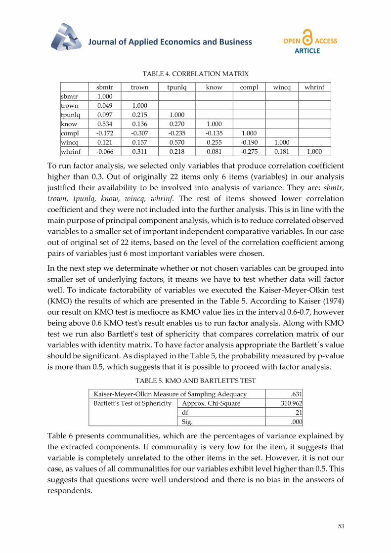
Journal of Applied Economics and Business
53
TABLE 4. CORRELATION MATRIX
sbmtr trown tpunlq know compl wincq whrinf
sbmtr 1.000
trown 0.049 1.000
tpunlq 0.097 0.215 1.000
know 0.534 0.136 0.270 1.000
compl -0.172 -0.307 -0.235 -0.135 1.000
wincq 0.121 0.157 0.570 0.255 -0.190 1.000
whrinf -0.066 0.311 0.218 0.081 -0.275 0.181 1.000
To run factor analysis, we selected only variables that produce correlation coefficient
higher than 0.3. Out of originally 22 items only 6 items (variables) in our analysis
justified their availability to be involved into analysis of variance. They are: sbmtr,
trown, tpunlq, know, wincq, whrinf. The rest of items showed lower correlation
coefficient and they were not included into the further analysis. This is in line with the
main purpose of principal component analysis, which is to reduce correlated observed
variables to a smaller set of important independent comparative variables. In our case
out of original set of 22 items, based on the level of the correlation coefficient among
pairs of variables just 6 most important variables were chosen.
In the next step we determinate whether or not chosen variables can be grouped into
smaller set of underlying factors, it means we have to test whether data will factor
well. To indicate factorability of variables we executed the Kaiser-Meyer-Olkin test
(KMO) the results of which are presented in the Table 5. According to Kaiser (1974)
our result on KMO test is mediocre as KMO value lies in the interval 0.6-0.7, however
being above 0.6 KMO test's result enables us to run factor analysis. Along with KMO
test we run also Bartlett's test of sphericity that compares correlation matrix of our
variables with identity matrix. To have factor analysis appropriate the Bartlett´s value
should be significant. As displayed in the Table 5, the probability measured by p-value
is more than 0.5, which suggests that it is possible to proceed with factor analysis.
TABLE 5. KMO AND BARTLETT'S TEST
Kaiser-Meyer-Olkin Measure of Sampling Adequacy .631
Bartlett's Test of Sphericity Approx. Chi-Square 310.962
df 21
Sig. .000
Table 6 presents communalities, which are the percentages of variance explained by
the extracted components. If communality is very low for the item, it suggests that
variable is completely unrelated to the other items in the set. However, it is not our
case, as values of all communalities for our variables exhibit level higher than 0.5. This
suggests that questions were well understood and there is no bias in the answers of
respondents.

Jana Kubicová, Barbora Valková
Factors of the Tax Reporting Compliance of the Slovak Residents
54 JOURNAL OF APPLIED ECONOMICS AND BUSINESS, VOL. 4, ISSUE 4 - DECEMBER, 2016, PP. 43-62
TABLE 6. COMMUNALITIES
Initial Extraction
sbmtr 1.000 0.813
trown 1.000 0.578
tpunlq 1.000 0.771
know 1.000 0.724
compl 1.000 0.534
wincq 1.000 0.785
whrinf 1.000 0.557
Extraction Method: Principal Component Analysis.
The purpose of principal component analysis is to explain as much variance as
possible by using as few components as possible. Components are extracted based on
the initial eigenvalues criterion, and components with eigenvalue more than 1.0 are
chosen for further analysis. Information how much of the variable in the data has been
explained by the extracted factors is reported in the Table 7. It shows three chosen
components based on the initial eigenvalues, their values are 2,309 for component 1,
then 1,386 for component 2, and 1,066 for component 3. All three chosen components
explain altogether cumulatively 68.027% of total variance, and each of them separately
explains approximately from 22.0-23.0% of variance.
TABLE 7. TOTAL VARIANCE EXPLAINED
Component Initial Eigenvalues Extraction Sums of Squared
Loadings
Rotation Sums of Squared
Loadings
Total % of
Variance
Cumulative
%
Total % of
Variance
Cumulative
%
Total % of
Variance
Cumulative
%
1 2,309 32,990 32,990 2,309 32,990 32,990 1,604 22,921 22,921
2 1,386 19,802 52,792 1,386 19,802 52,792 1,597 22,810 45,732
3 1,066 15,235 68,027 1,066 15,235 68,027 1,561 22,295 68,027
4 0,721 10,302 78,329
5 0,676 9,653 87,982
6 0,439 6,273 94,255
7 0,402 5,745 100,000
Extraction Method: Principal Component Analysis.
Initial levels of eigenvalue serve us as critical measure when determining how many
components should be chosen to process analysis. Other tool is to visualize
information on eigenvalue levels. Scree plot is useful graph which plots number of
components on x-axis and eigenvalues on y-axis. To indicate an appropriate number
of components we look at the inflation point located in the elbow of the curve. In our
case we chose three components, the same number as decided by checking
eigenvalues expressed in numerical form. Figure 1 presents the plot of eigenvalues.

Journal of Applied Economics and Business
55
FIG. 1 SCREE PLOT
Component matrix shown in Table 8 presents only chosen components - those with
initial eigenvalues more than 1.0. It displays factor loadings when values are
unrotated.
TABLE 8. COMPONENT MATRIX
Component
1 2 3
tpunlq 0.713 -0.101 0.502
wincq 0.676 0.572
compl -0.564 0.223 0.408
trown 0.519 -0.376 -0.408
sbmtr 0.427 0.735 -0.301
know 0.595 0.598 -0.117
whrinf 0.469 -0.536 -0.223
Extraction Method: Principal Component Analysis.
a. 3 components extracted.
Rotated component matrix displayed by Table 9, shows how each variable loads into
each component. We can see high numbers in component 1 and at the same time low
or no numbers of those variables in component two and three. Contrary, high
numbers for variables in component two are accompanied with low or no values of
those variables in the component one and three.

Jana Kubicová, Barbora Valková
Factors of the Tax Reporting Compliance of the Slovak Residents
56 JOURNAL OF APPLIED ECONOMICS AND BUSINESS, VOL. 4, ISSUE 4 - DECEMBER, 2016, PP. 43-62
TABLE 9. ROTATED COMPONENT MATRIXA
Component
1 2 3
trown 0.755
whrinf 0.707 0.185 -0.151
compl -0.695 -0.210
wincq 0.875 0.109
tpunlq 0.189 0.852
sbmtr 0.901
know 0.247 0.810
Extraction Method: Principal Component Analysis, Rotation Method:
Varimax with Kaiser Normalization, a, Rotation converged in 4 iterations
Component plot presented in the rotated space is a graphical help summarizing
everything shown in previous tables (Figure 2).
FIG. 2 COMPONENT PLOT IN ROTATED SPACE
CONCLUSION
Our factor analysis results allow us to identify and name some hidden factors that
determine tax-reporting compliance of individuals - residents of Slovakia. According
to our factor analysis there are three hidden factors of tax compliance of individuals -
residents of Slovakia. Below we describe these three dimensions in order of their
importance.
Component 1: Tax Complexity and Information. This dimension represents 22.921%
of the total variance. It consists of three items trown, whrinf, compl. Individuals who
submit tax return themselves (trown, +), where they find information (whrinf, +) and
degree of complexity of tax return form (compl, -). Our results are consistent with
previous empirical research, for example with the finding, that tax compliance is
Journal of Applied Economics and Business
57
negatively related to complexity of tax returns (Bhattacharjee et al, 2015) and
positively related to the accessibility of tax related information (Devos et al, 2015;
Kosonen et al, 2015; Phillips, 2014). This result is in line with considerations of the EU
which promoted settling up central one-stop-shop in tax administration where cross-
border workers could seek reliable tax information (European Commision, 2015).
This finding implies, that in attempts to enhance tax compliance of individuals who
reside in Slovakia, tax policy makers should pay closer attention on tax complexity
and publication form, accessibility and easiness of tax related information.
Component 2: Tax Literacy. This dimension represents 22.810% of the total variance,
and with component 1 it explains 45.732% of the total variance cumulatively. This
component consists of two items: wincq and tpunlq. They focus on taxpayers'
knowledge of tax law, especially on those tax law provisions that provide rules and
requirements on income disclosure and obligation to submit tax return also by
individuals who earn income abroad. One question asks about the meaning of the
concept world income (wincq, +), and the second question checks whether respondents
understand clearly meaning of the concept of the taxpayer with unlimited tax liability
(tpunlq, +). Component 2 suggests that tax compliance of individuals who work
abroad is closely linked and positively influenced by depth of knowledge of the tax
law provisions and regulations. Our finding is consistent with findings in other
empirical research studies (Gangl et al, 2014; Nichita, 2015; Rhoades; 1999). Policy
implication is, that to improve tax compliance, Slovak government, including tax
administration, should pay appropriate attention to quality education of individuals
in the field of tax requirements.
Component 3: Foreign Income Level and Knowledge. This dimension represents
22.295% of the total variance, and together with other two components it explains
65.027% of the total variability. It consists of two items. First, responses on question
whether individual taxpayer submitted tax return to declare income above 1,800 Euro
earned abroad in previous tax year (sbmtr, +). Disclosure of foreign income earned
abroad by individual taxpayers certainly increases tax compliance. It is interesting that
this item is combined with item which examines whether individual taxpayers know
that they have to submit tax return even if they earn income only abroad (know, +).
Both items together indicate that individuals with higher income and more
knowledgeable tend more likely to comply with tax obligations. This finding implies,
that to boost tax compliance, Slovak government should pay more attention not only
to higher income taxpayers, but also to individuals with lower income.
Our research proves that both, economic and behavioral factors, play important role
in enhancing tax compliance of Slovak individuals who earn income abroad.

Jana Kubicová, Barbora Valková
Factors of the Tax Reporting Compliance of the Slovak Residents
58 JOURNAL OF APPLIED ECONOMICS AND BUSINESS, VOL. 4, ISSUE 4 - DECEMBER, 2016, PP. 43-62
ACKNOWLEDGMENT
This paper is result of the research project No VEGA 1/0776/16 funded by the scheme
of the Ministry of Education of the Slovak Republic. Relevance of the content of the
paper to the project VEGA 1/0776/16 is 1.0.
REFERENCES
Alabede, J. O., Ariffin, Z. Z. & Md Idris, K. (2011). Public Governance Quality and Tax
Compliance Behavior in Nigeria: The Moderating Role of Financial Condition and
Risk Preference, Issues In Social & Environmental Accounting, 5(1/2), 3-24.
Allingham, M. & Sandmo, A. (1972). Income Tax Evasion: A Theoretical Analysis,
Journal of Public Economics, 1(3-4), 323-338.
Alon, A. & Hageman, A. (2013). The Impact of Corruption on Firm Tax Compliance in
Transition Economies: Whom Do You Trust?, Journal of Business Ethics, 116(3), 479-
494.
Andor, L. (2014). Labor Mobility in the EU (public speach).
Azwadi, A. & Norsiah, A. (2014). Trust and Tax Compliance Among Malaysian
Working Youth, International Journal of Public Administration, 37(7), 389-396.
Bătrâncea, L. M., Nichita, R. A., Bătrâncea, I. & Moldovan, B. A. (2012). Tax
Compliance Models: from Economic to Behavioral Approaches, 36, 13-25.
Benk, S., Çakmak, A. F. & Budak, T. (2011). An Investigation Of Tax Compliance
Intention: A Theory of Planned Behavior Approach, European Journal of Economics,
Finance and Administrative Sciences, 28, 181-188.
Benk, S., Budak, T. & Cakmak, A. F. (2012). Tax Professionals' Perceptions of Tax
Fairness: Survey Evidence in Turkey, International Journal of Business and Social
Science, 3(2), 112-116.
Bernasconi, M. (1998). Tax Evasion and Orders of Risk Aversion, Journal of Public
Economics, 67, 123-134.
Bhattacharjee, S., Moreno, K. & Salbado, D. A. (2015). The Impact of Multiple Tax
Returns on Tax Compliance Behavior, Behavioral Research in Accounting, 27(1), 99-
119.
Blumental, M., Christian, C. & Slemrod, J. (1998). The Determinants of Income Tax
Compliance: Evidence from a Controlled Experiment in Minnesota, WP 6575.
Brink, W. D. & White, R. A. (2015). The Effects of a Shared Interest and Regret Salience
on Tax Evasion, Journal of the American Taxation Association, 37(2), 109-135.
Bruttel, L. & Friehe, T. (2014). On the path dependence of tax compliance, European
Economic Review, 65, 90-107.

Journal of Applied Economics and Business
59
Comrey, A. L. & Lee, H. B. (1992). First Course in Factor Analysis, Hillsdale, NJ :
Erlbaum.
Devos, K. & Zackrisson, M. (2015). Tax compliance and the public disclosure of tax
information: An Australia/Norway comparison, Ejournal Of Tax Research, 13(1), 108.
Doerrenberg, P. & Peichl, A. (2010). Progressive Taxation and Tax Morale, IZA
Discussion Paper No 5378.
Durham, Y., Manly, T. S. & Ritsema, C. (2014). The Effects of Income Source, Context,
And Income Level on Tax Compliance Decisions in a Dynamic Experiment, Journal of
Economic Psychology, 40220-233.
Erard, B. & Feinstein, J. S. (1994). Honesty and Evasion in the Tax Compliance Game,
RAND Journal of Economics, 25(1), 1-19.
Eurobarometer Survey. (2014). www-ec.europa.eu. [Online].
European Commision. (2015). Direct Tax Cross-Border Problems Affecting Citizens.
EC. Taxation and custom Union. [Online]
http://ec.europa.eu/taxation_customs/taxation/ personal_tax/crossborder-
issues/index_en.htm#actions
European Commission. (2012). Commission to examine tax measures for cross-border
workers. Press release IP/12/340. s.l. : European Commission, 2012.
http://europa.eu/rapid/press-release_IP-12-340_en.htm.
European Parliament. (2015). Free movement of workers. European Parliament at
Your Service. [Online] 2015. http://www.europarl.europa.eu/atyourservice/en/
displayFtu.html?ftuId=FTU_3.1.3.html.
Eurostat. (2014). Labour Market and Labour Force Survey. Statistics. Foreign workers
in the EU. Eurostat. [Online] http://ec.europa.eu/eurostat
/statistics-explained/ index.php/Labour_market_and_Labour_forcesurvey_%28LFS%
29_statistics#Foreign_workers_in_the_EU.
Eze, U. C. (2014). Determinants of Tax Compliance of Corporate Taxpayers in
Malaysia, eJournal of Tax Research, 12(2), 383-410.
Friedland, N., Maital, S. & Rutenberg, A. (1978). A Simulation Study of Income Tax
Evasion, Journal of Public Economics, 10, 107-116.
Gahramanov, E. (2009). The Theoretical Analysis of Income Tax Evasion Revisited,
Economic Issues, 14(1), 35-40.
Gangl, K., Torgler, B., Kirchler, E. & Hofmann, E. (2014). Effects of supervision on tax
compliance: Evidence from a field experiment in Austria, Economics Letters, 123(3),
378-380.

Jana Kubicová, Barbora Valková
Factors of the Tax Reporting Compliance of the Slovak Residents
60 JOURNAL OF APPLIED ECONOMICS AND BUSINESS, VOL. 4, ISSUE 4 - DECEMBER, 2016, PP. 43-62
Giachi, S. (2014). Social Dimensions of Tax Evasion: Trust and Tax Morale in
Contemporary Spain, Revista Española De Investigaciones Sociologicas, 145, 73-96.
Gideon, Y. (2009). The Tax Compliance Demand Curve: A Diagrammatical Approach
to Income Tax Evasion, Journal of Economic Education, 40(2), 213-224.
Gordon, J. P. F. (1989). Individual Morality and Reputation Costs as Deterrence to Tax
Evasion, European Economic Review, l(4), 797-805.
Gorsuch, R. L. (1983). Factor Analysis, Hillsdale, NJ: Erlbaum.
Gulyás, L., Máhr, T. & Tóth, I. J. (2015). Factors to curb Tax Evasion: Evidence from
the TAXSIM Agent-Based Simulation Model, Hungarian Academy of Sciences, Centre
for Economic and Regional Studies. Discussion Papers, MT-DP_2015/21.
Hageman, B. D. A. & Kelliher, C. (2013). Analyzing the Role of Social Norms in Tax
Compliance Behavior, Journal of Business Ethics, 115(3), 451-468.
Hallsworth, M. (2014). The use of field experiments to increase tax compliance, Oxford
Review of Economic Policy, 30(4), 658-679.
Hauptman, L., Gürarda, S. & Korez-Vlde, R. (2015). Exploring Voluntary Tax
Compliance Factors in Slovenia: Implications for Tax Administration and
Policymakers, Lex Localis - Journal Of Local Self-Government, 13(3).
İnam, S. N. B. & Murat, D. (2014). Factors Affecting Tax Compliance of Taxpayers: The
Role of Tax Officer - the Case of Istanbul and Canakkale.
Iyer, G. S., Reckers, P. M. J. & Sanders, D. L. (2010). Increasing Tax Compliance in
Washington State: A Field Experiment, National Tax Journal, 63(1), 7-32.
Kirchler, E. (2007). The Economic Psychology of Tax Behavior. Cambridge: Cambridge
University Press.
Kirchler, E., Hoelzl, E. & Wahl, I. (2008). Enforced versus Voluntary Tax Compliance:
The "Slippery Slope" Framework, 29(2), 210-225.
Kirchler, E., Kogler, C. & Muehlbacher, S. (2014). Cooperative Tax Compliance: From
Deterrence to Deference. Current Directions, Psychological Science, 23(2), 87-92.
Kogler, C., Bătrâncea, L., Nichita, A., Pantya, J., Belianin, A. & Kirchler, E. (2013). Trust
and power as determinants of tax compliance: Testing the assumptions of the slippery
slope framework in Austria, Hungary, Romania and Russia, Journal of Economic
Psychology, 34169-34180.
Kosonen, T. & Ropponen, O. (2015). The role of information in tax compliance:
Evidence from a natural field experiment, Economics Letters, 129, 18-21.
Kudrle, R. T. (2012). Whose "Treasure Islands"? The Role of Tax Havens in the Global
Economy, Special Reports, 69-80.

Journal of Applied Economics and Business
61
Lesnik, T., Kracun, D. & Jagric, T. (2014). Recession and Tax Compliance - The Case of
Slovenia, Engineering Economics, 25(2), 130-140.
Lisi, G. (2015). Tax morale, tax compliance and the optimal tax policy, Economic
Analysis & Policy, 45(1), 27-32.
Ministry of Foreign Affairs of the Slovak Republic. (2014). Koncepcia štátnej politiky
Slovenskej republiky vo vzťahu k slovákom žijúcim v zahraničí na obdobie rokov 2016
– 2020. www.justice.gov.sk. [Online].
Muehlbacher, S. & Kirchler, E. (2010). Tax Compliance by Trust and Power of
Authorities, International Economic Journal, 24(4), 607-610.
Nichita, R. A. (2015). Knowledge is Power. Improving Tax Compliance by Means of
Boosting Tax Literacy, Annals of the University of Oradea, Economic Science Series,
24, 87-88.
Office for National Statistics. (2015). Annual Population Survey Household Dataset,
January - December, 2013. Social Survey Division, Office for National Statistic.
London: UK Data Service.
Oğuz, A. M. & Özgür, İ. (2013). An Agent-Based Analysis of Tax Compliance for
Turkey, Anadolu University Journal of Social Sciences, 13(2), 143-152.
Phillips, M. D. (2014). Individual Income Tax Compliance And Information Reporting:
What Do The U.S. Data Show?, National Tax Journal, 67(3), 531-556.
Rhoades, S. C. (1999). The Impact of Multiple Component Reporting on Tax
Compliance and Audit Strategies, Accounting Review, 74(1), 63-85.
Plumley, A. H. (1996). The Determinants of Individual Income Tax Compliance:
Estimating The Impacts of Tax Policy, Enforcement, and IRS Responsiveness.
Washington, DC: IRS Publication 1916 (Rev.11-96).
Sandmo, A. (2004). The Theory of Tax Evasion: A Retrospective View, Norwegian
School of Economics and Business Administration, Discussion Paper 31/04, 1-31.
Serim, N., İnam, B. & Murat, D. (2014). Factors Affecting Tax Compliance of
Taxpayers: The Role of Tax Officer The Case of Istanbul and Canakkale, Business &
Economics Research Journal, 5(2), 19-32.
Torgler, B. (2002). Speaking to Theorists and Searching for Facts: Tax Morale and Tax
Compliance in Experiments, Journal of Economic Surveys, 16(5), 657-683.
Sour, L. (2004). An Economic Model of Tax Compliance with Individual Morality and
group Conformity, Economía Mexicana Nueva Época, XIII, Primer Semestre, 43-61.

Jana Kubicová, Barbora Valková
Factors of the Tax Reporting Compliance of the Slovak Residents
62 JOURNAL OF APPLIED ECONOMICS AND BUSINESS, VOL. 4, ISSUE 4 - DECEMBER, 2016, PP. 43-62
Feld, L. P. & Frey, B. S. (2007). Tax Compliance as the Result of a Psychological Tax
Contract: The Role of Incentives and Responsive Regulation, Law and Policy, 29(1),
103-120.
Witte, A. D., Tauchen, H. & Hall, G. (1987). Tax Compliance Research: Models, Data
and Methods, American Statistical Association, Proceedings of the Survey Research
Methods Section, 101-107.
Wu , S. Y. & Teng, M. J. (2005). Determinants of Tax Compliance - A Cross-Country
Analysis, Public Finance Analysis, 61(3), 393-417.
Yamala, G. O. & Gumus, E. (2013). Determinants of Tax Evasion Behavior: Empirical
Evidence from Survey Data, International Business and Management, 6(2), 15-23.
Yitzaki, S. (1974). A Note on Income Tax Evasion: A Theoretical Analysis, 3(2), 201-
202.