Parametric Equations for Curves in Space

76

CHAPTER 3

PARAMETRIC EQUATIONS FOR CURVES IN SPACE

At this point we’ve talked an awful lot about graphs of functions of two variables and

also about graphing surfaces in both cylindrical and spherical coordinates, and we’ve

looked at an incredible number of examples of the kinds of surfaces that we can

generate. However, sometimes it’s not really a surface at all that we want to describe.

Sometimes we just want to describe a curve or path that something like a baseball

might travel when thrown. How do we do that? Well, the easiest way is usually to

express the ball’s location in space as a function of time. When we do this, we think

of time, t, as a parameter for determining location of our object in coordinates

( , , )x y z . Consequently, we need our variables x, y, and z to all be expressed as

functions of t. When we specify all three functions as well as the range of values for

t, then we call the result our parametric equations for the curve that, in this case, our

baseball will travel.

Now let’s look at a simple example. Below are some parametric equations followed

by the curve they produce.

cos( )sin(5 )

50 30

x ty t

tz

t

==

=

≤ ≤

Parametric Equations for Curves in Space

77

Well, that looks pretty disgusting! The good news is that we won’t really need to

know how to do very many parametrizations. In fact, there are only three things we’ll

need to know how to do well: (1) how to construct parametric equations for a line, (2)

how to construct parametric equations for a circle, and (3) how to construct

parametric equations for a cross-section of certain types of planes with a surface.

Let’s begin with the circle.

Fotunarely, you probably already know how to parametrize a circle – you just don’t

know that you know. Nevertheless, if you think back to trigonometry and polar

coordinates, then you’ll recall that for a circle of radius 1 with center at the origin, we

have cosx θ= and siny θ= where 0 2θ π≤ ≤ . We can also think of these equations

Parametric Equations for Curves in Space

78

as parametric equations where the parameter is θ . If we graph the corresponding

curve in 2-dimensions, then we get our unit circle.

In this case, if we start with 0θ = and end with 2θ π= , then we’ll trace our circle in

the counterclockwise direction both starting and ending at the point ( )1,0 . Much later

on, we’ll designate the counterclockwise direction as the positive direction, and we’ll

be very concerned about which direction our curve is traced in. For now, however, it

won’t be that much of a concern for us. One of the things we do want to take note of

at this point, though, is that there will always exist an infinite number of

parametrizations for any particular curve. For example, if in our parametric equations

above, we replace θ by 2θ and change the range for θ to 0 4θ π≤ ≤ , then the end

result is the same.

Parametric Equations for Curves in Space

79

cos( 2)sin( 2)

0 4

xy

θθ

θ π

==≤ ≤

If we want to graph this circle in 3-dimensions but keep it in the xy-plane, then all we

have do is to add the coordinate 0z = . By the way, at this point I’m going to switch

to using t for the parameter.

cos( )sin( )0

0 2

x ty tz

t π

===≤ ≤

Parametric Equations for Curves in Space

80

And if we want to elevate this circle to 4z = , all we have to do is change the fixed

value of z to four.

cos( )sin( )4

0 2

x ty tz

t π

===≤ ≤

Parametric Equations for Curves in Space

81

A fun variation we can do of a circle is a spiral that is technically known as a helix.

However, I like to call it a slinky. To make a helix (or slinky), set your parametric

equations so that x and y describe a circle, and then let z gradually increase as t

increases.

cos( )sin( )/10

0 10

x ty tz t

t π

===≤ ≤

Parametric Equations for Curves in Space

82

So that’s it for circles! Now let’s start looking at lines. Suppose you want to define a

line segment parametrically that starts at ( , , )a b c and ends at ( , , )u v w .

xΔyΔ

zΔ

( , , )a b c

( , , )u v w

xΔyΔ

zΔ

( , , )a b c

( , , )u v w

Parametric Equations for Curves in Space

83

Then I claim that the parametric equations are as follows:

0 1

x a t xy b t yz c t z

t

= + ⋅Δ= + ⋅Δ= + ⋅Δ≤ ≤

Certainly, when 0t = we are at the point ( , , )a b c , and when 1t = we add just the right

amount of change to x, y, and z to take us to the point ( , , )u v w . Also, note the

following two things. First, in our parametric equations we have x, y, and z all given

as linear functions of t. Furthermore, by contemplating the diagram above, we should

be able to convince ourselves that the object created by this parametrization will be a

line. For example, when 12

t = , we will arrive at half our total change for x, y, and z,

and the diagram suggests that we will have covered half the straight line distance

between ( , , )a b c and ( , , )u v w . Now let’s do a particular example.

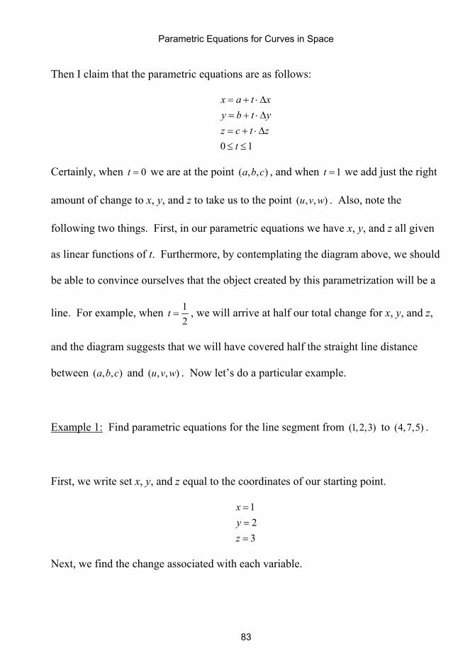
Example 1: Find parametric equations for the line segment from (1,2,3) to (4,7,5) .

First, we write set x, y, and z equal to the coordinates of our starting point.

123

xyz

===

Next, we find the change associated with each variable.

Parametric Equations for Curves in Space

84

4 1 37 2 55 3 2

xyz

Δ = − =Δ = − =Δ = − =

And finally, we multiply each change by t, add to our starting point, and let t vary

from 0 to 1.

1 32 53 2

0 1

x ty tz t

t

= += += +≤ ≤

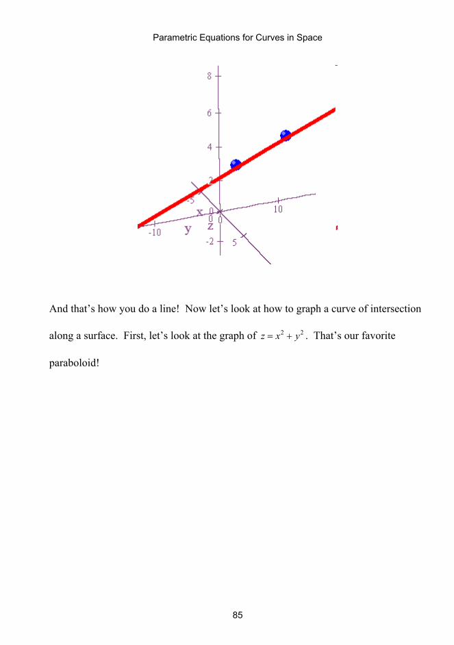
The end result is a very nice line segment from one point to another.

And if you want to extend the line, you just change the range for your parameter to

t−∞ < < ∞ .

Parametric Equations for Curves in Space

85

And that’s how you do a line! Now let’s look at how to graph a curve of intersection

along a surface. First, let’s look at the graph of 2 2z x y= + . That’s our favorite

paraboloid!

Parametric Equations for Curves in Space

86

Now let’s slice through this surface with the plane 2x = .

Parametric Equations for Curves in Space

87

The result is a nice, parabolic cross-section. As we’ve seen before, we can get the

equation for this cross-section by setting 2x = in our formula for the parabolid. This

gives us 2 2 22 4z y y= + = + . To now create a parametrization for this curve in 3-

dimensional space, one thing, at least, should be clear. We should fix x to the value 2.

And now the rest of it is really quite simple. Jut set y t= and then 24z t= + . This is

really just another way of saying that 24z y= + . And finally, for the range of values

of our parameter, for the graph above it will suffice to use 3 3t− ≤ ≤ since that is the

range I used in the graph for x and y. Okay, we’re now ready to look at the

parametric equations and the resulting graph.

Parametric Equations for Curves in Space

88

2

2

43 3

xy t

z tt

==

= +− ≤ ≤

Success! However, we can do even more. Suppose we look at the graph of our

cross-section 24z y= + in just 2-dimensions. Then we get something like the

following.

Parametric Equations for Curves in Space

89

If we set 1y = on this graph, then 24 1 5z = + = , and we can use standard calculus

techniques to find the slope of the tangent line to this curve at the point ( )1,5 .

Clearly, 2dz ydy

= and 1

2y

dzdy =

= . Thus, an equation for our tangent to this 2-

dimensional curve is 2( 1) 5 2 3z y y= − + = + .

Now the question we want to ask ourselves is can we easily move all of this back

onto our 3-dimensional surface, and the answer is yes, if we define our tangent line

parametrically. First of all, since our point in 2-dimensions was ( ) ( ), 1,5y z = and

since we want everything to wind up in the plane 2x = , the point on the surface at

which we want to place our tangent line is ( ) ( ), , 2,1,5x y z = . Second, since the slope

of our tangent line in 2-dimensions was 2, in our parametric equations all we need to

Parametric Equations for Curves in Space

90

do is make sure that z grows twice as fast as y. All of this will happen perfectly if we

set our parametric equations to:

215 2

xy tz t

t

== += +

−∞ < < ∞

Notice that these are parametric equations for a line that passes through ( )2,1,5 , the x-

value is permanently fixed at 2 which will put our line in the plane 2x = , and z grows

twice as fast as y. Now let’s look at the result.

Parametric Equations for Curves in Space

91

Perfect! Now let’s do exactly the same thing, but this time we’ll fix the y-value.

Since the point at which we want to construct a tangent line to the surface is ( )2,1,5 ,

we’ll intersect our surface with the plane 1y = .

So far so good! Now let’s add the graph of the cross-section to the surface. In this

case, we’ll have 2 2 21 1z x x= + = + , and so our parametric equations should be:

2

1

13 3

x ty

z tt

==

= +− < <

Parametric Equations for Curves in Space

92

Most excellent! Now let’s see if we can add the tangent line to the point ( )2,1,5 that

lies in the plane 1y = . To get the slope of the tangent line, we’ll consider 2 1z x= + as

a function of one variable and differentiate to get 2dz xdx

= . If we evaluate this

derivative at 2x = , we get that the slope of our tangent line is 4. We don’t really

need to construct the equation in 2-dimensions as we did previously since all we need

is the slope in order to finish setting up parametric equations for the line in 3-

dimensions. Just remember that, in this problem, if x increases by t, then z has to

increase by 4t so that the slope of the line will be 4. And the parametric equations for

this second tangent line at the point ( )2,1,5 are:

Parametric Equations for Curves in Space

93

215 4

x tyz t

t

= +== +

−∞ < < ∞

Ah, yes, perfection is a beautiful thing! If we now, however, look at the graph of our

original parabolid with only the two tangent lines at the point ( )2,1,5 , then we might

notice something very important. Namely, these two lines define a unique plane that

is tangent to our surface at the point ( )2,1,5 . As we proceed through this book this

notion of a tangent plane will become increasingly important as it is simply the higher

dimensional version of the tangent line that you undoubtedly studied in first semester

calculus.

Parametric Equations for Curves in Space

94

Parametric Equations for Curves in Space

95

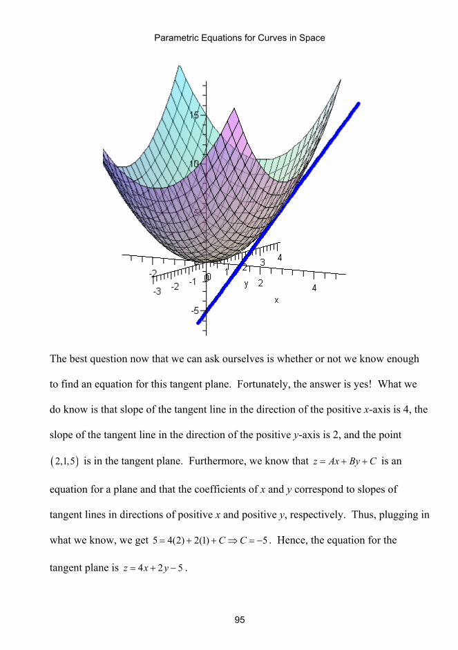
The best question now that we can ask ourselves is whether or not we know enough

to find an equation for this tangent plane. Fortunately, the answer is yes! What we

do know is that slope of the tangent line in the direction of the positive x-axis is 4, the

slope of the tangent line in the direction of the positive y-axis is 2, and the point

( )2,1,5 is in the tangent plane. Furthermore, we know that z Ax By C= + + is an

equation for a plane and that the coefficients of x and y correspond to slopes of

tangent lines in directions of positive x and positive y, respectively. Thus, plugging in

what we know, we get 5 4(2) 2(1) 5C C= + + ⇒ = − . Hence, the equation for the

tangent plane is 4 2 5z x y= + − .

Parametric Equations for Curves in Space

96

Parametric Equations for Curves in Space

97

I love it when a construction comes together!