3D STABILITY ANALYSIS OF CONCAVE SLOPES IN...

IJST, Transactions of Civil Engineering, Vol. 36, No. C2, pp 181-194 Printed in The Islamic Republic of Iran, 2012 © Shiraz University

3D STABILITY ANALYSIS OF CONCAVE SLOPES IN PLAN VIEW USING LINEAR FINITE ELEMENT

AND LOWER BOUND METHOD*

A. TOTONCHI1**, F. ASKARI2 AND O. FARZANEH3 1Dept. of Civil Eng., Science and Research Branch, Islamic Azad University, Tehran, I. R. of Iran

Email: [email protected] 2Iran International Earthquake Engineering Institute, Tehran, I. R. of Iran

3Dept. of Civil Engineering, Tehran University, Tehran, I. R. of Iran

Abstract– It is well known that the plan curvature of curved slopes has an influence on the stability of the slopes. This paper aims to present a method of three-dimensional stability analysis of concave slopes in plan view based on the Lower-bound theorem of the limit analysis approach. The method’s aim is to determine the factor of safety of such slopes using numerical linear finite element and lower bound limit analysis method to produce some stability charts for three dimensional (3D) homogeneous concave slopes. Although the conventional two and three dimension limit equilibrium method (LEM) is used more often in practice for evaluating slope stability, the accuracy of the method is often questioned due to the underlying assumptions that it makes. The rigorous limit analysis results in this paper were found to be closely conservative results to exact solutions and therefore can be used to benchmark for solutions from other methods. It was found that using a two dimensional (2D) analysis to analyze a 3D problem will lead to a significant difference in the factors of safety depending on the slope geometries. Numerical 3D results of the proposed algorithm are presented in the form of some dimensionless graphs, which can be a convenient tool for use by practicing engineers to estimate the initial stability for excavated or man-made slopes. The results obtained using this 3D method show that the stability of concave slopes in plan view increases as the relative curvature R/H and the relative width of slope decrease.

Keywords– Three-dimensional slope, slope stability, limit analysis, lower-bound, limit equilibrium

1. INTRODUCTION

Most analyses for slope stability have dealt with straight slopes with a planar surface. However, there are many concave slopes in plan view with nonplanar surfaces. During the past decades, the influence of plan curvature on the stability of slopes has been investigated mainly by Leshchinsky and Baker [1], Giger and Krizek [2,3], Baker and Leshchinsky [4], Xing [5], and Ohlmacher [6] for some special cases. Giger and Krizek [2, 3] used the upper-bound theorem of limit analysis to study the stability of a vertical corner cut subjected to a local load. They assumed a kinematically admissible collapse mechanism and, through a formal energy formulation, assessed the stability with respect to shear strength of soil. Leshchinsky et al. [7] presented a 3D analysis of slope stability based on the variational limiting equilibrium approach and proved that it can be considered as a rigorous upper bound in limit analysis. Leshchinsky and Baker [1] used a modified solution of the approach mentioned to study 3D end effects on the stability of homogeneous slopes constrained in the third direction and applied it to investigate the stability of vertical Received by the editors April 20, 2011; Accepted June 21, 2011. Corresponding author

A. Totonchi et al.

IJST, Transactions of Civil Engineering, Volume 36, Number C2 August 2012

182

corner cuts. Using a variational approach, Baker and Leshchinsky [4] discussed the stability of conical heaps formed by homogeneous soils. Xing [5] proposed a 3D stability analysis for concave slopes in plan view using the equilibrium concept. Based on the limit equilibrium method, Ohlmacher [6] investigated a case study including concave and concave slopes.

Michalowski [8] introduced a rigorous 3D approach in the strict framework of limit analysis for homogeneous and straight slopes. In his analysis, the geometry of slope and slip surface was unrestricted and both cohesive and frictional soils were included. Farzaneh and Askari [9] improved Michalowski’s algorithm in the case of 3D homogeneous slopes and extended it to analyze the stability of nonhomogeneous slopes.

In most cases it is not feasible to perform a full displacement finite element analysis and as such the three dimensional effects of the slope in question are often ignored. However, ignoring the 3D effects when analyzing slopes can lead to unsafe answers. In the back analyses of shear strengths, for example, neglecting the 3D effects will lead to values that are too high, and therefore affect any further stability assessments at the same location. As stated previously, one aim of this study is to produce 3D stability charts that can be used by practicing engineers, extending those currently used regularly for 2D slope stability evaluation.

This paper is devoted to use linear finite element, lower-bound solution method and an optimization approach to make the maximum lower bound solutions for 3D concave slope stability. The main purpose of this paper is to provide sets of 3D stability charts for homogeneous soil slopes by using the finite element lower bounding method which can be used to benchmark for solutions from other methods.

2. BACKGROUND The limit analysis method models the soil as a perfectly plastic material obeying an associated flow rule [25]. With this idealization of the soil behavior, two plastic bounding theorems (lower and upper bounds) can be proved. The lower bound theorem states if an equilibrium distribution of stress covering the whole body can be found that balances a set of external loads on the stress boundary and is nowhere above the failure criterion of the material, the external loads are not higher than the true collapse loads. It is noted that in the lower bound theorem, the strain and displacements are not considered and that the state of stress is not necessarily the actual state of stress at collapse. By examining different admissible states of stress, the best (highest) lower bound value may be found.

Although the limit theorems provide a simple and useful way of analyzing the stability of geotechnical structures, they have not been widely applied to the 3D slope stability problem. Currently, most slope stability evaluations based on the limit theorems have used the upper bound method alone, such as Chen et al. [11,12], Donald and Chen [13], Farzaneh and Askari [9, 10], De Buhan and Garnier [14], Michalowski [8,15], and Viratjandr and Michalowski [16]. Major contributions for soil slope stability analysis were presented by Michalowski and his co-worker who investigated local footing load effects on the 3D slope stability [8] and provided sets of stability charts for cohesive-frictional slopes which took seismic loadings and pore pressure into account. In addition, Michalowski [17] employed the limit analysis technique to estimate the stability of uniformly reinforced slopes.

Because of the difficulties of constructing statically admissible stress fields manually, the application of limit analysis has in the past almost exclusively concentrated on the upper bound method. In fact, the authors are not aware of any rigorous lower bound solutions for the stability of slopes in cohesive-frictional soils. Although the upper bound solutions may be used as an estimate for the true collapse load, it is the lower bound solutions that are generally more useful in practice, because they are inherently conservative.

3D stability analysis of concave slopes in plan view…

August 2012 IJST, Transactions of Civil Engineering, Volume 36, Number C2

183

A lower bound solution is obtained by insisting that the stresses obey equilibrium and satisfy both the stress boundary conditions and the yield criterion. Each of these requirements imposes a separate set of constraints on the nodal stresses. In the lower bound finite-element analysis, statically admissible stress discontinuities are permitted at edges shared by adjacent triangles and also along borders between adjacent rectangular extension elements. The finite element lower bound limit analysis techniques developed by Lyamin and Sloan [18] and Krabbenhoft et al. [19] provide a useful method for dealing with the problems of slope stability. These numerical lower bound methods have been used to provide chart solutions by Yu et al. [20] for 2D purely cohesive and cohesive-frictional soil slopes. In this paper, similar formulations are used and described with new types of elements for investigating the effect of concavity in slopes.

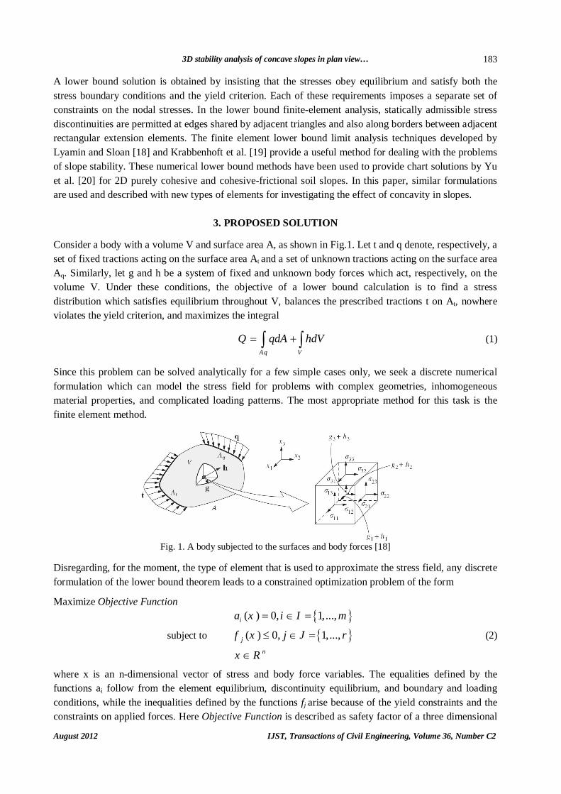
3. PROPOSED SOLUTION Consider a body with a volume V and surface area A, as shown in Fig.1. Let t and q denote, respectively, a set of fixed tractions acting on the surface area At and a set of unknown tractions acting on the surface area Aq. Similarly, let g and h be a system of fixed and unknown body forces which act, respectively, on the volume V. Under these conditions, the objective of a lower bound calculation is to find a stress distribution which satisfies equilibrium throughout V, balances the prescribed tractions t on At, nowhere violates the yield criterion, and maximizes the integral

Aq V

Q qdA hdV (1)

Since this problem can be solved analytically for a few simple cases only, we seek a discrete numerical formulation which can model the stress field for problems with complex geometries, inhomogeneous material properties, and complicated loading patterns. The most appropriate method for this task is the finite element method.

Fig. 1. A body subjected to the surfaces and body forces [18]

Disregarding, for the moment, the type of element that is used to approximate the stress field, any discrete formulation of the lower bound theorem leads to a constrained optimization problem of the form Maximize Objective Function

subject to

( ) 0, 1,...,

( ) 0, 1,...,i

j

n

a x i I m

f x j J r

x R

(2)

where x is an n-dimensional vector of stress and body force variables. The equalities defined by the functions ai follow from the element equilibrium, discontinuity equilibrium, and boundary and loading conditions, while the inequalities defined by the functions fj arise because of the yield constraints and the constraints on applied forces. Here Objective Function is described as safety factor of a three dimensional

A. Totonchi et al.


184

slope and ai is a global matrix which contains equilibrium, discontinuity and boundary equations. In addition, fj produces the conditions in which nodal stresses will be less than the yield surface. Maximizing Objective Function leads to using an optimization approach. In this paper the nonlinear optimization based on a fast quasi-Newton method whose iteration count is largely independent of the mesh refinement, is selected for finding the maximum lower-bound solution of safety factor which satisfies the element equilibrium, discontinuity equilibrium, and boundary and loading conditions. The global form of each element in this solution is shown in Fig. 2. As is seen, the stresses variation between each node of the element is assumed to be linear, thus this type of finite element is called Linear Finite Element. The following section gives a detailed description of the discretization procedure for the case of 3-dimensional linear elements. There are strong reasons for choosing linear finite elements, and not higher order finite elements, for lower bound computations.

Fig. 2. Global form of elements

Unlike the usual form of the finite element method in which each node is unique to a particular element, multiple nodes can share the same coordinates, and statically admissible stress discontinuities are permitted at all inter-element boundaries. The typical 3D slope geometry details for the problem of this paper are shown in Fig. 3.

Fig. 3. Geometry details of problem (a). Plan (b). Section A-A

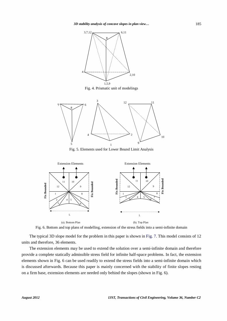
In this paper, all models are organized from some prismatic units as is shown in Fig. 4. Using this

type of unit as a base of modelling, all kinds of straight, convex, concave and every other arbitrary shape in plan view of slopes can be created. Each discussed unit is combined from three volumetric pyramid elements which are shown in Fig. 5.

The global form of modelling consists of two plans, one which is located at the top and the other at the bottom of the model. Figure 6. shows the top and bottom plans of modelling. Between each pair of slices in the plans (1 to 12), 3 elements in the form of a prismatic unit shown in Fig. 4 are constituted. For higher slopes, various numbers of prismatic units are used in the height of the slopes.

L A A

H

β

(a)

(b)

1 2

3

4



185

Fig. 4. Prismatic unit of modelings

Fig. 5. Elements used for Lower Bound Limit Analysis

Fig. 6. Bottom and top plans of modelling, extension of the stress fields into a semi-infinite domain

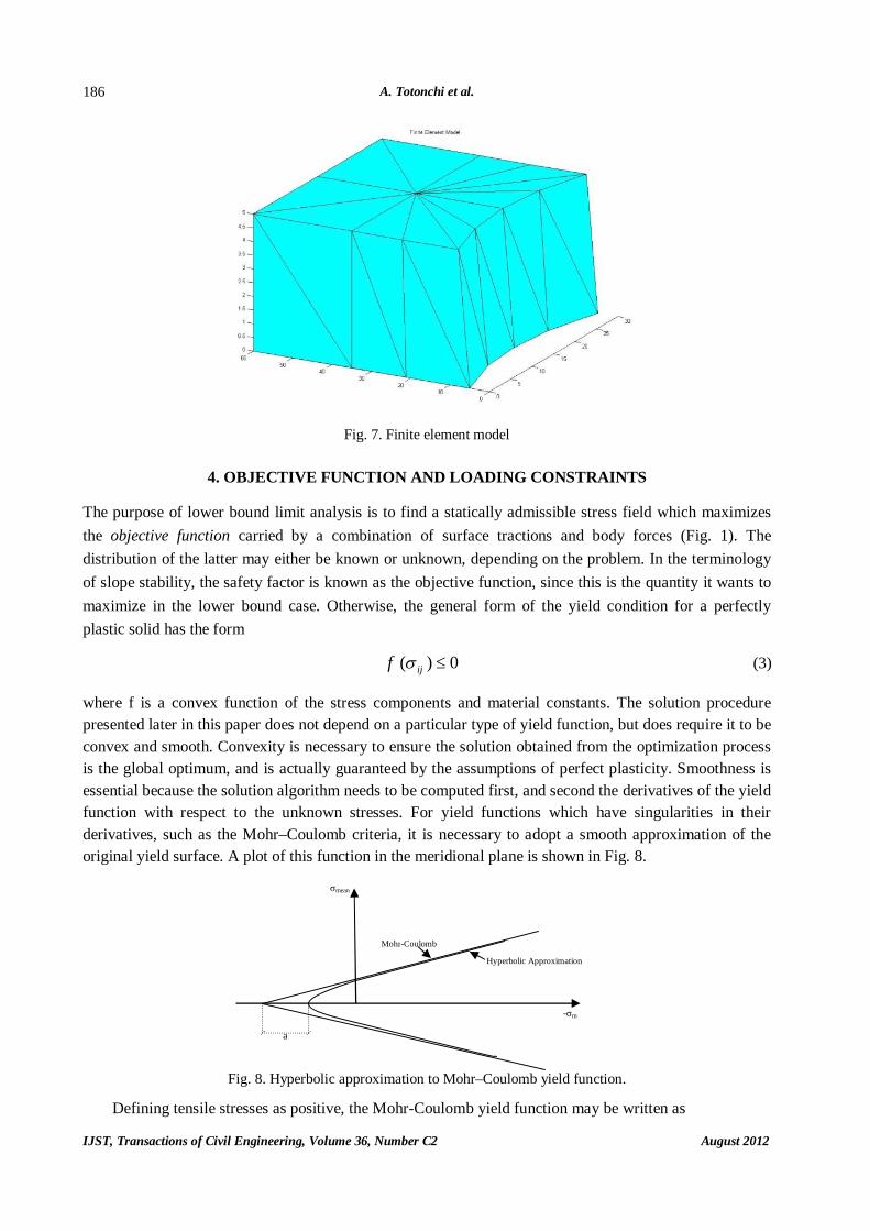
The typical 3D slope model for the problem in this paper is shown in Fig. 7. This model consists of 12

units and therefore, 36 elements. The extension elements may be used to extend the solution over a semi-infinite domain and therefore

provide a complete statically admissible stress field for infinite half-space problems. In fact, the extension elements shown in Fig. 6 can be used readily to extend the stress fields into a semi-infinite domain which is discussed afterwards. Because this paper is mainly concerned with the stability of finite slopes resting on a firm base, extension elements are needed only behind the slopes (shown in Fig. 6).

1

2 3

4 5 6

7

8

12

11 10

9

Fix

Bou

nded

Fix

Bou

nded

Extension Elements

L

(b). Top Plan

1 2

3 4 5

6 7

8

9

10 11

12

L

Fix

Bou

nded

Fix

Bou

nded

Extension Elements

(a). Bottom Plan

1

4

3

2

8 6 7

5

12 11

10

9

1,5,9

2,10 4

3,7,12

8

6,11

A. Totonchi et al.


186

Fig. 7. Finite element model

4. OBJECTIVE FUNCTION AND LOADING CONSTRAINTS

The purpose of lower bound limit analysis is to find a statically admissible stress field which maximizes the objective function carried by a combination of surface tractions and body forces (Fig. 1). The distribution of the latter may either be known or unknown, depending on the problem. In the terminology of slope stability, the safety factor is known as the objective function, since this is the quantity it wants to maximize in the lower bound case. Otherwise, the general form of the yield condition for a perfectly plastic solid has the form

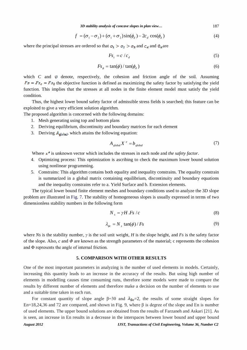
( ) 0ijf (3) where f is a convex function of the stress components and material constants. The solution procedure presented later in this paper does not depend on a particular type of yield function, but does require it to be convex and smooth. Convexity is necessary to ensure the solution obtained from the optimization process is the global optimum, and is actually guaranteed by the assumptions of perfect plasticity. Smoothness is essential because the solution algorithm needs to be computed first, and second the derivatives of the yield function with respect to the unknown stresses. For yield functions which have singularities in their derivatives, such as the Mohr–Coulomb criteria, it is necessary to adopt a smooth approximation of the original yield surface. A plot of this function in the meridional plane is shown in Fig. 8.

Fig. 8. Hyperbolic approximation to Mohr–Coulomb yield function.

Defining tensile stresses as positive, the Mohr-Coulomb yield function may be written as

σmean

a

Hyperbolic Approximation

Mohr-Coulomb

-σm



187

1 2 1 2( ) ( )sin( ) 2 cos( )d d df c (4) where the principal stresses are ordered so that and and are

/c dFs c c (5)

tan( ) / tan( )dFs (6) which C and denote, respectively, the cohesion and friction angle of the soil. Assuming

the objective function is defined as maximizing the safety factor by satisfying the yield function. This implies that the stresses at all nodes in the finite element model must satisfy the yield condition.

Thus, the highest lower bound safety factor of admissible stress fields is searched; this feature can be exploited to give a very efficient solution algorithm. The proposed algorithm is concerned with the following domains:

1. Mesh generating using top and bottom plans 2. Deriving equilibrium, discontinuity and boundary matrices for each element 3. Deriving , which attains the following equation:

e

global globalA X b (7)

Where is unknown vector which includes the stresses in each node and the safety factor. 4. Optimizing process: This optimization is ascribing to check the maximum lower bound solution

using nonlinear programming. 5. Constrains: This algorithm contains both equality and inequality constrains. The equality constrain

is summarized in a global matrix containing equilibrium, discontinuity and boundary equations and the inequality constrains refer to a. Yield Surface and b. Extension elements.

The typical lower bound finite element meshes and boundary conditions used to analyze the 3D slope problem are illustrated in Fig. 7. The stability of homogeneous slopes is usually expressed in terms of two dimensionless stability numbers in the following form

. /sN H Fs c (8)

tan( ) /c sN Fs (9) where Ns is the stability number, γ is the soil unit weight, H is the slope height, and Fs is the safety factor of the slope. Also, c and Φ are known as the strength parameters of the material; c represents the cohesion and Φ represents the angle of internal friction.

5. COMPARISON WITH OTHER RESULTS One of the most important parameters in analyzing is the number of used elements in models. Certainly, increasing this quantity leads to an increase in the accuracy of the results. But using high number of elements in modelling causes time consuming runs, therefore some models were made to compare the results by different number of elements and therefore make a decision on the number of elements to use and a suitable time taken in each run.

For constant quantity of slope angle β=30 and =2, the results of some straight slopes for En=18,24,36 and 72 are compared, and shown in Fig. 9, where β is degree of the slope and En is number of used elements. The upper bound solutions are obtained from the results of Farzaneh and Askari [21]. As is seen, an increase in En results in a decrease in the interspaces between lower bound and upper bound

A. Totonchi et al.


188

solutions. This means that by increasing En, the accuracy of the results increases but the rate decreases, as Fig. 9 shows. Therefore it can be concluded that for higher number of elements, the difference between results can be connivance. Thus in this paper, all numerical results are made of 36 elements because of the low rate of variations afterwards (Each run takes approximately 12 minutes).

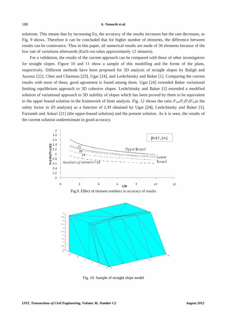
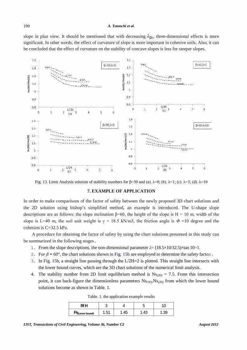
For a validation, the results of the current approach can be compared with those of other investigators for straight slopes. Figure 10 and 11 show a sample of this modelling and the forms of the plans, respectively. Different methods have been proposed for 3D analysis of straight slopes by Baligh and Azzouz [22], Chen and Chameau [23], Ugai [24], and Leshchinsky and Baker [1]. Comparing the current results with most of these, good agreement is found among them. Ugai [24] extended Baker variational limiting equilibrium approach to 3D cohesive slopes. Leshchinsky and Baker [1] extended a modified solution of variational approach in 3D stability of slopes which has been proved by them to be equivalent to the upper bound solution in the framework of limit analysis. Fig. 12 shows the ratio F3D/F2D (FiDis the safety factor in iD analysis) as a function of L/H obtained by Ugai [24], Leshchinsky and Baker [1], Farzaneh and Askari [21] (the upper-bound solution) and the present solution. As it is seen, the results of the current solution underestimate in good accuracy.

Fig.9. Effect of element numbers in accuracy of results

Fig. 10. Sample of straight slope model



189

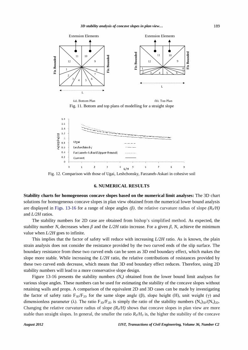
Fig. 11. Bottom and top plans of modelling for a straight slope

Fig. 12. Comparison with those of Ugai, Leshchonsky, Farzaneh-Askari in cohesive soil

6. NUMERICAL RESULTS

Stability charts for homogeneous concave slopes based on the numerical limit analyses: The 3D chart solutions for homogeneous concave slopes in plan view obtained from the numerical lower bound analysis are displayed in Figs. 13-16 for a range of slope angles (β), the relative curvature radius of slope (R0/H) and L/2H ratios.

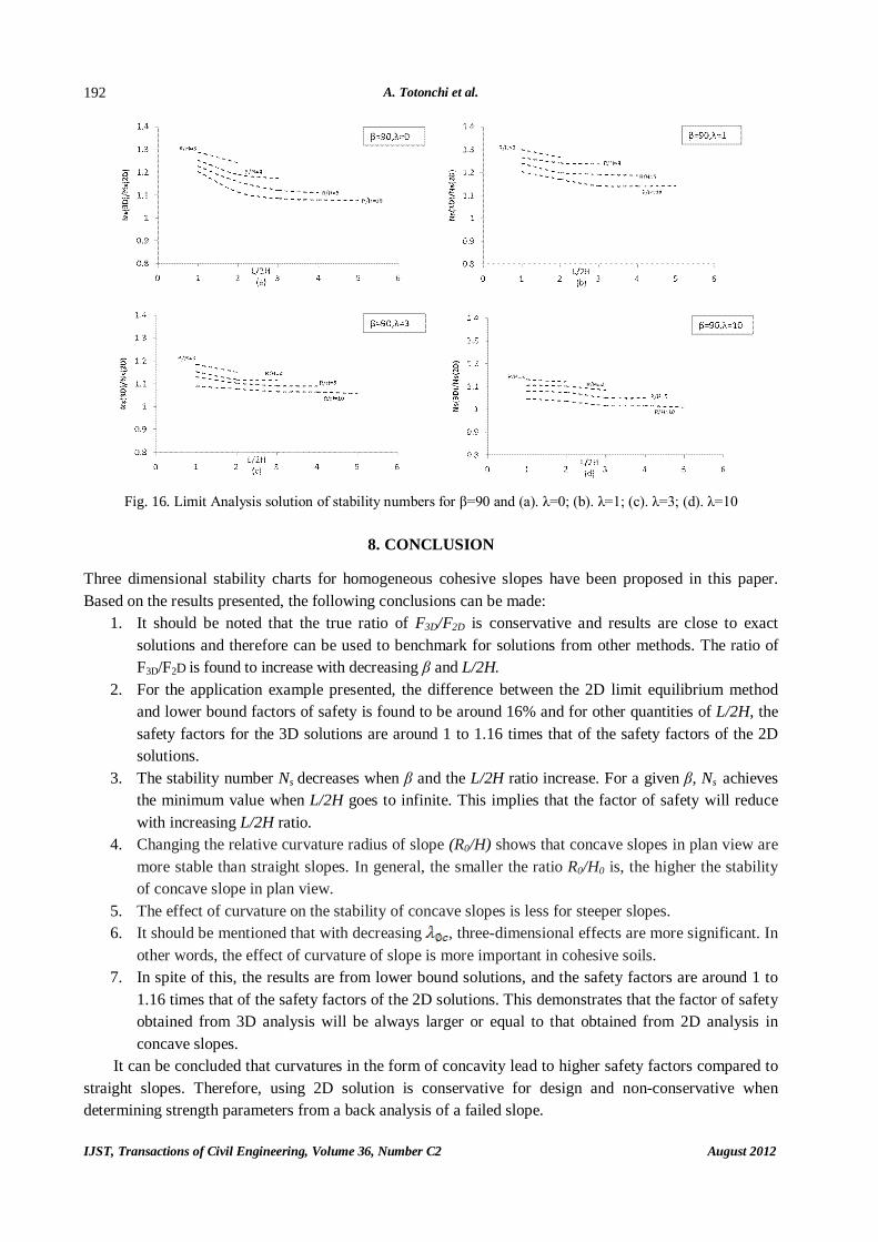
The stability numbers for 2D case are obtained from bishop’s simplified method. As expected, the stability number Ns decreases when β and the L/2H ratio increase. For a given β, Ns achieve the minimum value when L/2H goes to infinite.

This implies that the factor of safety will reduce with increasing L/2H ratio. As is known, the plain strain analysis does not consider the resistance provided by the two curved ends of the slip surface. The boundary resistance from these two curved ends can be seen as 3D end boundary effect, which makes the slope more stable. While increasing the L/2H ratio, the relative contributions of resistances provided by these two curved ends decrease, which means that 3D end boundary effect reduces. Therefore, using 2D stability numbers will lead to a more conservative slope design.

Figure 13-16 presents the stability numbers (Ns) obtained from the lower bound limit analyses for various slope angles. These numbers can be used for estimating the stability of the concave slopes without retaining walls and props. A comparison of the equivalent 2D and 3D cases can be made by investigating the factor of safety ratio F3D/F2D for the same slope angle (β), slope height (H), unit weight (γ) and dimensionless parameter (λ). The ratio F3D/F2D is simply the ratio of the stability numbers (Ns)3D/(Ns)2D. Changing the relative curvature radius of slope (R0/H) shows that concave slopes in plan view are more stable than straight slopes. In general, the smaller the ratio R0/H0 is, the higher the stability of the concave

1

2 3 4 5 6

7 8

12

11 10

9

Fix

Bou

nded

Fix

Bou

nded

Extension Elements

L

(b). Top Plan

1 2 3 4 5 6 7

8

9

10 11

12

L

Fix

Bou

nded

Fix

Bou

nded

Extension Elements

(a). Bottom Plan

A. Totonchi et al.


190

slope in plan view. It should be mentioned that with decreasing , three-dimensional effects is more significant. In other words, the effect of curvature of slope is more important in cohesive soils. Also, it can be concluded that the effect of curvature on the stability of concave slopes is less for steeper slopes.

Fig. 13. Limit Analysis solution of stability numbers for β=30 and (a). λ=0; (b). λ=1; (c). λ=3; (d). λ=10

7. EXAMPLE OF APPLICATION

In order to make comparisons of the factor of safety between the newly proposed 3D chart solutions and the 2D solution using bishop’s simplified method, an example is introduced. The U-shape slope descriptions are as follows: the slope inclination β=60, the height of the slope is H = 10 m, width of the slope is L=40 m, the soil unit weight is γ = 18.5 kN/m3, the friction angle is Φ =10 degree and the cohesion is C=32.5 kPa.

A procedure for obtaining the factor of safety by using the chart solutions presented in this study can be summarized in the following stages.

1. From the slope descriptions, the non-dimensional parameter λ= (18.5×10/32.5)×tan 10=1. 2. For β = 60°, the chart solutions shown in Fig. 15b are employed to determine the safety factor. 3. In Fig. 15b, a straight line passing through the L/2H=2 is plotted. This straight line intersects with

the lower bound curves, which are the 3D chart solutions of the numerical limit analysis. 4. The stability number from 2D limit equilibrium method is Ns(2D) = 7.5. From this intersection

point, it can back-figure the dimensionless parameters Ns(3D)/Ns(2D) from which the lower bound solutions become as shown in Table. 1.

Table. 1. the application example results

R/H 3 4 5 10

Fs(Lower bound) 1.51 1.45 1.43 1.39



191



As seen, the lower bound safety factors of R/H=3,4,5 and 10 for L/2H =2 are 1.51, 1.45, 1.43 and 1.39; respectively. In spite of this, the results are from lower bound solutions, and the safety factors are around 1 to 1.16 times that of the safety factors of the 2D solutions. This demonstrates that the factor of safety obtained from 3D analysis will always be larger or equal to that obtained from 2D analysis in concave slopes. It can also be concluded that curvatures in the form of concavity leads to higher safety factors in comparison to straight slopes. Therefore, using 2D solution is conservative for design and non-conservative when determining strength parameters from a back analysis of a failed slope. In addition, the difference between the 2D limit equilibrium method and lower-bound factors of safety for this example is found to be around 17%. This difference decreases slightly when the ratio of L/2H increases.

A. Totonchi et al.


192


8. CONCLUSION

Three dimensional stability charts for homogeneous cohesive slopes have been proposed in this paper. Based on the results presented, the following conclusions can be made:

1. It should be noted that the true ratio of F3D/F2D is conservative and results are close to exact solutions and therefore can be used to benchmark for solutions from other methods. The ratio of F3D/F2D is found to increase with decreasing β and L/2H.

2. For the application example presented, the difference between the 2D limit equilibrium method and lower bound factors of safety is found to be around 16% and for other quantities of L/2H, the safety factors for the 3D solutions are around 1 to 1.16 times that of the safety factors of the 2D solutions.

3. The stability number Ns decreases when β and the L/2H ratio increase. For a given β, Ns achieves the minimum value when L/2H goes to infinite. This implies that the factor of safety will reduce with increasing L/2H ratio.

4. Changing the relative curvature radius of slope (R0/H) shows that concave slopes in plan view are more stable than straight slopes. In general, the smaller the ratio R0/H0 is, the higher the stability of concave slope in plan view.

5. The effect of curvature on the stability of concave slopes is less for steeper slopes. 6. It should be mentioned that with decreasing , three-dimensional effects are more significant. In

other words, the effect of curvature of slope is more important in cohesive soils. 7. In spite of this, the results are from lower bound solutions, and the safety factors are around 1 to

1.16 times that of the safety factors of the 2D solutions. This demonstrates that the factor of safety obtained from 3D analysis will be always larger or equal to that obtained from 2D analysis in concave slopes.

It can be concluded that curvatures in the form of concavity lead to higher safety factors compared to straight slopes. Therefore, using 2D solution is conservative for design and non-conservative when determining strength parameters from a back analysis of a failed slope.



193

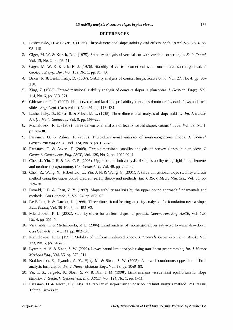
REFERENCES 1. Leshchinsky, D. & Baker, R. (1986). Three-dimensional slope stability: end effects. Soils Found, Vol. 26, 4, pp.

98–110. 2. Giger, M. W. & Krizek, R. J. (1975). Stability analysis of vertical cut with variable corner angle. Soils Found,

Vol. 15, No. 2, pp. 63–71. 3. Giger, M. W. & Krizek, R. J. (1976). Stability of vertical corner cut with concentrated surcharge load. J.

Geotech. Engrg. Div., Vol. 102, No. 1, pp. 31–40. 4. Baker, R. & Leshchinsky, D. (1987). Stability analysis of conical heaps. Soils Found, Vol. 27, No. 4, pp. 99–

110. 5. Xing, Z. (1988). Three-dimensional stability analysis of concave slopes in plan view. J. Geotech. Engrg, Vol.

114, No. 6, pp. 658–671. 6. Ohlmacher, G. C. (2007). Plan curvature and landslide probability in regions dominated by earth flows and earth

slides. Eng. Geol. (Amsterdam), Vol. 91, pp. 117–134. 7. Leshchinsky, D., Baker, R. & Silver, M. L. (1985). Three-dimensional analysis of slope stability. Int. J. Numer.

Analyt. Meth. Geomech., Vol. 9, pp. 199–223. 8. Michalowski, R. L. (1989). Three dimensional analysis of locally loaded slopes. Geotechnique, Vol. 39, No. 1,

pp. 27–38. 9. Farzaneh, O. & Askari, F. (2003). Three-dimensional analysis of nonhomogeneous slopes. J. Geotech

Geoenviron Eng ASCE, Vol. 134, No. 8, pp. 137–45. 10. Farzaneh, O. & Askari, F. (2008). Three-dimensional stability analysis of convex slopes in plan view. J.

Geotech. Geoenviron. Eng. ASCE, Vol. 129, No. 2, pp. 1090-0241. 11. Chen, J., Yin, J. H. & Lee, C. F. (2003). Upper bound limit analysis of slope stability using rigid finite elements

and nonlinear programming. Can Geotech. J., Vol. 40, pp. 742–52. 12. Chen, Z., Wang, X., Haberfield, C., Yin, J. H. & Wang, Y. (2001). A three-dimensional slope stability analysis

method using the upper bound theorem part I: theory and methods. Int. J. Rock. Mech. Min. Sci., Vol. 38, pp. 369–78.

13. Donald, I. B. & Chen, Z. Y. (1997). Slope stability analysis by the upper bound approach:fundamentals and methods. Can Geotech. J., Vol. 34, pp. 853–62.

14. De Buhan, P. & Garnier, D. (1998). Three dimensional bearing capacity analysis of a foundation near a slope. Soils Found, Vol. 38, No. 3, pp. 153–63.

15. Michalowski, R. L. (2002). Stability charts for uniform slopes. J. geotech. Geoenviron. Eng. ASCE, Vol. 128, No. 4, pp. 351–5.

16. Viratjandr, C. & Michalowski, R. L. (2006). Limit analysis of submerged slopes subjected to water drawdown. Can Geotech. J., Vol. 43, pp. 802–14.

17. Michalowski, R. L. (1997). Stability of uniform reinforced slopes. J. Geotech. Geoenviron. Eng. ASCE, Vol. 123, No. 6, pp. 546–56.

18. Lyamin, A. V. & Sloan, S. W. (2002). Lower bound limit analysis using non-linear programming. Int. J. Numer Methods Eng., Vol. 55, pp. 573–611.

19. Krabbenhoft, K., Lyamin, A. V., Hjiaj, M. & Sloan, S. W. (2005). A new discontinuous upper bound limit analysis formulation. Int. J. Numer Methods Eng., Vol. 63, pp. 1069–88.

20. Yu, H. S., Salgado, R., Sloan, S. W. & Kim, J. M. (1998). Limit analysis versus limit equilibrium for slope stability. J. Geotech. Geoenviron. Eng. ASCE, Vol. 124, No. 1, pp. 1–11.

21. Farzaneh, O. & Askari, F. (1994). 3D stability of slopes using upper bound limit analysis method. PhD thesis, Tehran University.

A. Totonchi et al.


194

22. Baligh, M. M. & Azzouz, A. S. (1975). End effects on stability of cohesive slopes. J. Geotech. Engrg. Div., Vol. 101, No. 11, pp. 1105–1117.

23. Chen, R. H. & Chameau, J. L. (1982). Three-dimensional limit equilibrium analysis of slopes. Geotechnique, Vol. 32, No. 1, pp. 31–40.

24. Ugai, K. (1985). Three-dimensional stability analysis of vertical cohesive slopes. Soils Found, Vol. 25, No. 3, pp. 41–8.

25. Jahanandish, M. & Eslami Haghighat, A. (2004). Analysis of Boundary value problems in soil Plasticity Assuming Non-Coaxiality, Iranian Journal of Science & Technology, Transaction B: Engineering, Vol. 28, No. B5.

3D STABILITY ANALYSIS OF CONCAVE SLOPES IN...

Documents

Transcript of 3D STABILITY ANALYSIS OF CONCAVE SLOPES IN...