3D Reconstruction of Buildings From Images with...

3D Reconstruction of Buildings From Images

with Automatic Facade Refinement

by

Christian Lindequist Larsen

Master’s Thesis in

Vision, Graphics and Interactive Systems

September 2009 – June 2010

Aalborg University

Department of Electronic Systems

Fredrik Bajers Vej 79220 Aalborg Ø

http://es.aau.dk/

Title:3D Reconstruction of BuildingsFrom Images with AutomaticFacade Refinement

Author:Christian Lindequist Larsen

Project Period:September 1, 2009 – June 3, 2010

Project Group:10gr1023

Supervisor:Thomas B. Moeslund

Copies:3

Report Pages:115

Total Pages:125

Attachments:1 CD

Abstract:

This project deals with the problem of recon-structing 3D models of real world buildingsfrom images. Potentially real estate marketingcan be improved by providing interactive visual-izations, e.g. on websites, of properties for sale.For this to be a viable option, however, simplermethods for 3D reconstruction are needed. Inparticular existing user assisted methods can beimproved by automating the process of addingfacade details to the reconstructed models.

In this project a proof of concept systemcovering the whole reconstruction process hasbeen developed. Structure and motion is re-covered from an unordered set of images of thebuilding to reconstruct, and this is followed byuser assisted reconstruction of a coarse textured3D model. The primary contribution in theproject is the development of a novel method forautomatic facade reconstruction, which whenapplied to the coarse model automatically addsfacade details such as recessed windows anddoors. The proposed method is based on an-alyzing the appearance of the facade, and thisis achieved using methods for image processingand pattern classification.

The results obtained from using the devel-oped system for reconstructing several refined3D models of buildings from images show thatthe proposed reconstruction method is suitablefor this purpose. The developed method for au-tomatic facade reconstruction on average cor-rectly detected and reconstructed 89% of re-cessed windows for the tested buildings. Somework remain for automatic facade reconstruc-tion to be fully automatic, e.g. the depth ofrecessed regions is specified by the user, butin general it is concluded that the proposedmethod leads to an improvement compared toexisting user assisted reconstruction methods.

Preface

This report constitutes the master’s thesis for Christian Lindequist Larsen,group 10gr1023 at the Vision, Graphics and Interactive Systems specializa-tion at Department of Electronic Systems, Aalborg University. The projecthas spanned the 9th and 10th semesters and extended from September 1, 2009to June 3, 2010.

References to secondary literature are specified using the syntax [number], wherethe number refers to the bibliography found at the end of the report, before theappendices. On the following page the vector and matrix notation used in thereport is introduced.

During the project a proof of concept system for reconstructing 3D models ofbuildings from images has been designed and implemented. The implementationprimarily consists of two applications written in C++, and various libraries havebeen used for specific tasks in the implementation. In particular OpenCV is usedfor image processing, and OpenGL is used for the user interface. Additionally,part of image processing is implemented using Matlab.

Further resources are available on the CD attached to this report. The contentsof this CD are:

• PDF version of this report.

• All test data and the obtained results.

• Implementation source code and documentation.

Aalborg – June 3, 2010

Christian Lindequist Larsen

v

Notation

Vectors are typeset in bold roman typeface, and are column vectors unless ex-plicitly transposed. A vector may appear in text as x = [x1 x2 x3]

T, which isequivalent to

x =

x1

x2

x3

.

Matrices are typeset using capital letters in roman typeface. For instance, a3 × 4 matrix P is defined as

P = [p1 p2 p3 p4] =

p11 p12 p13 p14

p21 p22 p23 p24

p31 p32 p33 p34

,

where the vectors pi, i = 1, . . . , 4 are the column vectors of the matrix. Zeroentries of matrices may be omitted to emphasize only the important elements,i.e. the following matrices are equivalent.

a b cd e

f

=

a b c0 d e0 0 f

vi

Contents

I Introduction 1

1 Motivation 3

1.1 Initiating Problem . . . . . . . . . . . . . . . . . . . . . . . . . . 5

2 Problem Analysis 7

2.1 Model Representation . . . . . . . . . . . . . . . . . . . . . . . . 7

2.2 Reconstruction Methods . . . . . . . . . . . . . . . . . . . . . . . 8

2.2.1 Manual . . . . . . . . . . . . . . . . . . . . . . . . . . . . 9

2.2.2 3D Scanning . . . . . . . . . . . . . . . . . . . . . . . . . 10

2.2.3 Photogrammetry . . . . . . . . . . . . . . . . . . . . . . . 12

2.3 Method Selection . . . . . . . . . . . . . . . . . . . . . . . . . . . 18

2.3.1 Data Acquisition . . . . . . . . . . . . . . . . . . . . . . . 18

2.3.2 Model Reconstruction . . . . . . . . . . . . . . . . . . . . 19

2.4 Conclusion . . . . . . . . . . . . . . . . . . . . . . . . . . . . . . 22

3 Problem Formulation 25

3.1 System Concept . . . . . . . . . . . . . . . . . . . . . . . . . . . 25

3.1.1 Method . . . . . . . . . . . . . . . . . . . . . . . . . . . . 26

3.2 Problem Delimitation . . . . . . . . . . . . . . . . . . . . . . . . 28

II Method 31

4 Preprocessing 33

4.1 Camera Model . . . . . . . . . . . . . . . . . . . . . . . . . . . . 33

4.1.1 Basic Pinhole Camera . . . . . . . . . . . . . . . . . . . . 33

4.1.2 Digital Cameras . . . . . . . . . . . . . . . . . . . . . . . 34

4.1.3 Camera Position and Orientation . . . . . . . . . . . . . . 35

4.2 Intrinsic Calibration . . . . . . . . . . . . . . . . . . . . . . . . . 36

4.2.1 Estimation from EXIF Data . . . . . . . . . . . . . . . . . 36

4.2.2 Evaluation . . . . . . . . . . . . . . . . . . . . . . . . . . 38

4.3 Detection of Keypoints . . . . . . . . . . . . . . . . . . . . . . . . 39

4.3.1 Comparison of SIFT and SURF . . . . . . . . . . . . . . . 39

4.3.2 Keypoint Detection Using SIFT . . . . . . . . . . . . . . 40

4.3.3 Evaluation . . . . . . . . . . . . . . . . . . . . . . . . . . 40

4.4 Conclusion . . . . . . . . . . . . . . . . . . . . . . . . . . . . . . 40

vii

Contents

5 Matching 43

5.1 Epipolar Geometry . . . . . . . . . . . . . . . . . . . . . . . . . . 43

5.2 Keypoint Matching . . . . . . . . . . . . . . . . . . . . . . . . . . 45

5.2.1 Evaluation . . . . . . . . . . . . . . . . . . . . . . . . . . 46

5.3 Estimation of the Fundamental Matrix . . . . . . . . . . . . . . . 46

5.3.1 The Normalized 8-Point Algorithm . . . . . . . . . . . . . 47

5.3.2 Random Sample Consensus (RANSAC) . . . . . . . . . . 49

5.3.3 Robust Estimation . . . . . . . . . . . . . . . . . . . . . . 51

5.3.4 Evaluation . . . . . . . . . . . . . . . . . . . . . . . . . . 51

5.4 Recovery of Relative Pose . . . . . . . . . . . . . . . . . . . . . . 53

5.4.1 Computing the Essential Matrix . . . . . . . . . . . . . . 54

5.4.2 Relative Pose from the Essential Matrix . . . . . . . . . . 54

5.4.3 Evaluation . . . . . . . . . . . . . . . . . . . . . . . . . . 55

5.5 Conclusion . . . . . . . . . . . . . . . . . . . . . . . . . . . . . . 56

6 Clustering 57

6.1 The First Pair of Images . . . . . . . . . . . . . . . . . . . . . . . 58

6.1.1 Triangulation of Keypoints . . . . . . . . . . . . . . . . . 58

6.2 Adding a Third Image . . . . . . . . . . . . . . . . . . . . . . . . 60

6.2.1 Initial Pose Estimate . . . . . . . . . . . . . . . . . . . . . 60

6.2.2 Recovering the Relative Scale . . . . . . . . . . . . . . . . 60

6.2.3 Triangulation of New Keypoints . . . . . . . . . . . . . . 62

6.2.4 Evaluation . . . . . . . . . . . . . . . . . . . . . . . . . . 63

6.3 The Clustering Algorithm . . . . . . . . . . . . . . . . . . . . . . 64

6.3.1 Maximum Spanning Trees . . . . . . . . . . . . . . . . . . 64

6.3.2 Building the Cluster . . . . . . . . . . . . . . . . . . . . . 65

6.3.3 Evaluation . . . . . . . . . . . . . . . . . . . . . . . . . . 68

6.4 Bundle Adjustment . . . . . . . . . . . . . . . . . . . . . . . . . . 68

6.4.1 Sparse Bundle Adjustment . . . . . . . . . . . . . . . . . 69

6.5 Optimization and Robustness . . . . . . . . . . . . . . . . . . . . 70

6.5.1 Evaluation . . . . . . . . . . . . . . . . . . . . . . . . . . 71

6.6 Conclusion . . . . . . . . . . . . . . . . . . . . . . . . . . . . . . 72

7 Coarse Model Reconstruction 75

7.1 User Assisted Reconstruction . . . . . . . . . . . . . . . . . . . . 75

7.1.1 Defining Locators . . . . . . . . . . . . . . . . . . . . . . . 76

7.1.2 Defining Polygons . . . . . . . . . . . . . . . . . . . . . . 76

7.1.3 Evaluation . . . . . . . . . . . . . . . . . . . . . . . . . . 76

7.2 Texture Extraction . . . . . . . . . . . . . . . . . . . . . . . . . . 78

7.2.1 Plane Fitting . . . . . . . . . . . . . . . . . . . . . . . . . 78

7.2.2 Computing Plane Axes . . . . . . . . . . . . . . . . . . . 79

7.2.3 Finding the Best Image . . . . . . . . . . . . . . . . . . . 80

7.2.4 Computing Vertex Projections . . . . . . . . . . . . . . . 81

7.2.5 Creating the Rectified Texture . . . . . . . . . . . . . . . 82

7.2.6 Evaluation . . . . . . . . . . . . . . . . . . . . . . . . . . 83

7.3 Conclusion . . . . . . . . . . . . . . . . . . . . . . . . . . . . . . 84

viii

Contents

8 Automatic Facade Reconstruction 858.1 Facade Segmentation . . . . . . . . . . . . . . . . . . . . . . . . . 85

8.1.1 Preprocessing . . . . . . . . . . . . . . . . . . . . . . . . . 868.1.2 Clustering and Classification . . . . . . . . . . . . . . . . 878.1.3 Noise Removal . . . . . . . . . . . . . . . . . . . . . . . . 908.1.4 BLOB Analysis . . . . . . . . . . . . . . . . . . . . . . . . 918.1.5 Evaluation . . . . . . . . . . . . . . . . . . . . . . . . . . 91

8.2 Finding Region Contours . . . . . . . . . . . . . . . . . . . . . . 928.3 Refining the Model . . . . . . . . . . . . . . . . . . . . . . . . . . 93

8.3.1 Evaluation . . . . . . . . . . . . . . . . . . . . . . . . . . 948.4 Conclusion . . . . . . . . . . . . . . . . . . . . . . . . . . . . . . 95

III Results and Discussion 97

9 System Evaluation 999.1 Test Data . . . . . . . . . . . . . . . . . . . . . . . . . . . . . . . 99

10 Structure from Motion 10110.1 Results . . . . . . . . . . . . . . . . . . . . . . . . . . . . . . . . . 10110.2 Discussion . . . . . . . . . . . . . . . . . . . . . . . . . . . . . . . 101

11 Coarse Model Reconstruction 10511.1 Results . . . . . . . . . . . . . . . . . . . . . . . . . . . . . . . . . 10511.2 Discussion . . . . . . . . . . . . . . . . . . . . . . . . . . . . . . . 105

12 Automatic Facade Reconstruction 10912.1 Results . . . . . . . . . . . . . . . . . . . . . . . . . . . . . . . . . 10912.2 Discussion . . . . . . . . . . . . . . . . . . . . . . . . . . . . . . . 109

13 Conclusion 11313.1 Discussion . . . . . . . . . . . . . . . . . . . . . . . . . . . . . . . 11413.2 Perspectives . . . . . . . . . . . . . . . . . . . . . . . . . . . . . . 115

Bibliography 117

IV Appendices 121

A Exchangeable Image File Format (EXIF) 123

B Least-Squares Solution of Homogeneous Equations 125

ix

Part I

Introduction

Chapter 1

Motivation

This is the era of computers. Today computers play an indispensable role insustaining the standard of living. Almost any man-made product that sur-rounds us has at some point been treated in digital form, whether it is duringdevelopment, production, marketing, or consumption. In development and pro-duction, computers make assisting technologies such as CAD/CAM1 available,and many products would be impossible to design and manufacture withoutthe help of computers. In marketing computers are used for both creating andpublishing product advertisements. For some groups of consumer products, e.g.electronic devices, it is even becoming the norm to order directly from shopson the internet, without having seen the product in real life. The informationavailable online about products is, in many cases, sufficient for the buyer tomake a considered decision as to which product to choose.

Common for the above examples is that computers help design, process, andpresent objects in the real world. To do this the objects must somehow be rep-resented in digital form. For many types of products the appearance is a keyselling point, and therefore they are presented visually in marketing material,both in printed and electronic advertisements. Typically this is done using prod-uct photographs, but for online product presentation more interactive optionsare available. An example of this is visualizing products interactively in 3D ona website, and in figure 1.1 two examples of this are shown using the HolomatixBlaze 3D software [3]. Using photorealistic rendering, the potential customergets a precise impression of the appearance of the product. Furthermore, theinteractivity allows the customer to inspect structure and details of the productthat might otherwise be hard to see in a product photograph.

Rendering a product photorealistically requires that a precise 3D model ofthe object including surface textures exists [36]. For products designed usingCAD such information is often readily available, as exact 3D models are a by-product of the process. The cell phone in figure 1.1a is an example of this. Butfor many products this is not the case, and the house in figure 1.1b is such anexample. In this situation it is necessary to somehow obtain a 3D model of theproduct, i.e. a digital representation, in order to present it interactively.

There are many ways to address the problem of reconstructing a 3D modelfrom a real world object, but it is often a cumbersome and time-consuming

1Computer-Aided Design (CAD), and Computer-Aided Manufacturing (CAM).

3

Chapter 1. Motivation

(a) (b)

Figure 1.1: Examples of interactive online 3D product presentations using the Holo-matix Blaze 3D software. The user can orbit around the product, and zoom in to takea closer look. a) Nokia 6300 cell phone [10]. b) Architectural visualization [3].

task. For instance the object can be reconstructed manually by taking mea-surements and using CAD tools for creating the 3D model, or laser scanningcould be employed to accurately measure the structure of the object [36]. Bothoptions are infeasible in many situations. For instance, manual modeling can bevery time-consuming depending on the desired level of detail, and laser scanningequipment is expensive and not available to layman. Therefore to make inter-active product presentations available for a wider range of products, a simplerapproach to 3D model reconstruction is necessary.

As mentioned above, one type of products for which 3D models typicallydo not exist is buildings. Real estate marketing material often includes a de-scription with information about the property, one or more photographs of theexterior and interior of the building, and a floor plan, see figure 1.2. Althoughthis provides a lot of useful information for the potential buyer, it is still notenough to really get a feeling of the property. If real estate agents could pro-vide an interactive virtual tour of properties for sale, e.g. as in the example infigure 1.1b, on their website, the potential customers would get an improvedexperience and have a better opportunity to get an impression of the buildingsbefore buying. Of course for real estate, this can never replace actually visitingthe property, but it may help making a decision which properties to take a lookat in person.

To make online interactive 3D presentations a viable option for real estateagents, 3D model reconstruction of buildings must be simplified compared tothe methods briefly mentioned above. This leads to the initiating problem ofthe project.

4

1.1. Initiating Problem

(a) (b)

Figure 1.2: A typical example of the visual presentation of a property for sale in realestate marketing material [2]. a) Photograph of the building. b) Floor plan.

1.1 Initiating Problem

The introduction has established that there is a need for simpler methods forreconstruction of 3D models from real world objects, which can be used for in-teractively presenting products e.g. on websites. In particular marketing of realestate, where 3D models of the buildings normally do no exist, could potentiallybenefit from this. Therefore the initiating problem of the project is as follows:

How is it possible to reconstruct a 3D model of a real world building,for interactive visualization, in a simple manner?

To answer this question, the initiating problem is analyzed in the followingchapter. This analysis then forms the basis for defining the specific problem ofthe project in chapter 3.

5

Chapter 2

Problem Analysis

The purpose of this chapter is to analyze the initiating problem defined insection 1.1. Based on this analysis the specific problem of the project is definedin the following chapter.

The key question in the initiating problem is how to reconstruct a 3D modelfrom a real world object, in this case a building. It is a prerequisite for answer-ing this question to know what is meant by 3D model, and this is defined insection 2.1 where different 3D model representations are analyzed. Then sec-tion 2.2 provides an analysis of different methods for 3D model reconstruction.Furthermore, the initiating problem asks for a 3D model for interactive visu-alization, which can be reconstructed in a simple manner. So in section 2.3,the method which best fits with the initiating problem is selected based on theanalysis of 3D model representations and reconstruction methods.

2.1 Model Representation

As discussed in chapter 1, to render an object photorealistically, a precise3D model including surface textures is required. That is the 3D model in-cludes both information about the 3D shape of the object and the appearanceof the object. Textures which are mapped to the surface of the object are typi-cally represented using images which can be extracted from photographs of theobject [36]. The main focus of the following analysis is how to represent theshape of the object.

The shape of a 3D model can be represented in different ways, and these rep-resentations can be categorized as: polygon mesh models, surface models, andsolid CAD models. The choice of representation depends on the data acquisitionmethod and the final purpose of the reconstructed model.

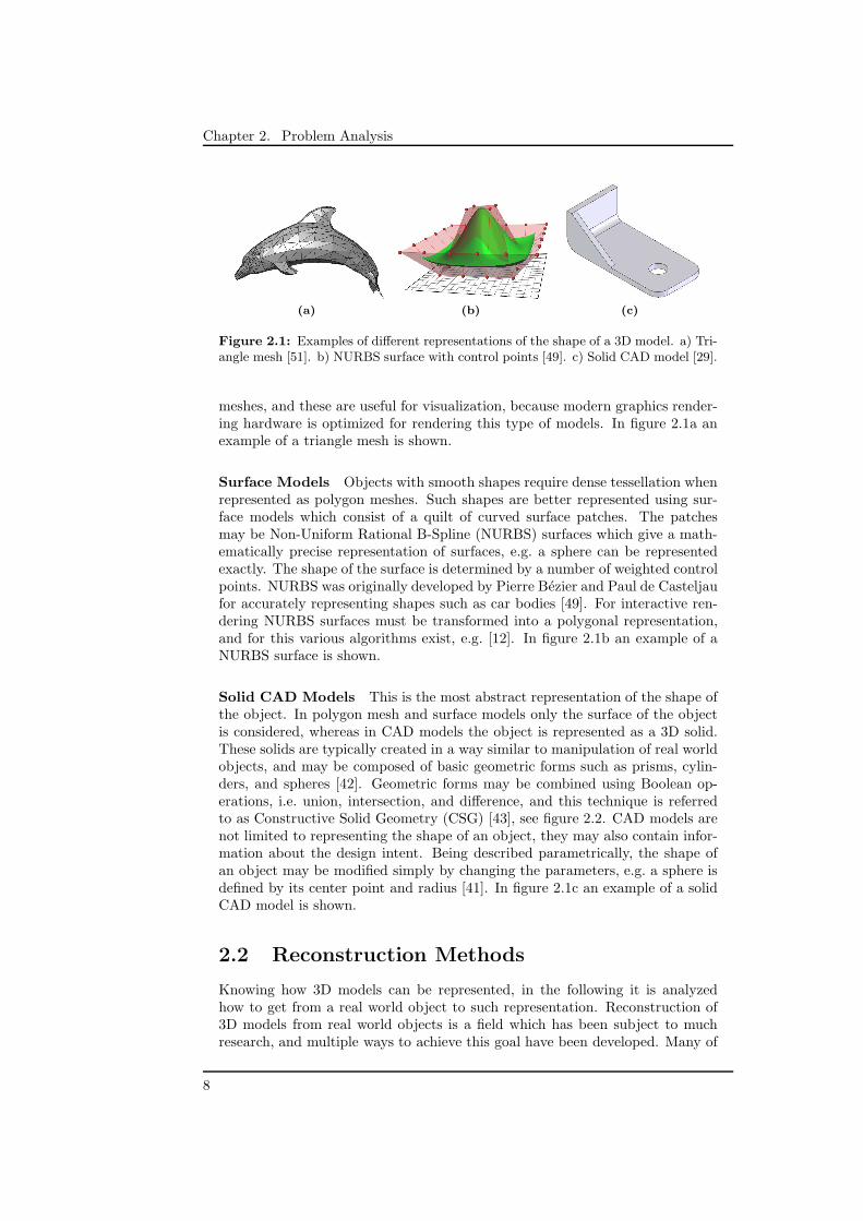
Polygon Mesh Models The shape of the object is represented using a col-lection of planar polygons referred to as faces. Faces are typically triangles,quadrilaterals, or simple convex polygons, but may be more complex such asconcave polygons or polygons with holes. The corners of the polygons are re-ferred to as vertices, and thus a polygon mesh is a collection of vertices, edges,and faces [51]. Curved surfaces are approximated using many small faceted sur-faces. Polygon mesh models having only triangle faces are referred to as triangle

7

Chapter 2. Problem Analysis

(a) (b) (c)

Figure 2.1: Examples of different representations of the shape of a 3D model. a) Tri-angle mesh [51]. b) NURBS surface with control points [49]. c) Solid CAD model [29].

meshes, and these are useful for visualization, because modern graphics render-ing hardware is optimized for rendering this type of models. In figure 2.1a anexample of a triangle mesh is shown.

Surface Models Objects with smooth shapes require dense tessellation whenrepresented as polygon meshes. Such shapes are better represented using sur-face models which consist of a quilt of curved surface patches. The patchesmay be Non-Uniform Rational B-Spline (NURBS) surfaces which give a math-ematically precise representation of surfaces, e.g. a sphere can be representedexactly. The shape of the surface is determined by a number of weighted controlpoints. NURBS was originally developed by Pierre Bezier and Paul de Casteljaufor accurately representing shapes such as car bodies [49]. For interactive ren-dering NURBS surfaces must be transformed into a polygonal representation,and for this various algorithms exist, e.g. [12]. In figure 2.1b an example of aNURBS surface is shown.

Solid CAD Models This is the most abstract representation of the shape ofthe object. In polygon mesh and surface models only the surface of the objectis considered, whereas in CAD models the object is represented as a 3D solid.These solids are typically created in a way similar to manipulation of real worldobjects, and may be composed of basic geometric forms such as prisms, cylin-ders, and spheres [42]. Geometric forms may be combined using Boolean op-erations, i.e. union, intersection, and difference, and this technique is referredto as Constructive Solid Geometry (CSG) [43], see figure 2.2. CAD models arenot limited to representing the shape of an object, they may also contain infor-mation about the design intent. Being described parametrically, the shape ofan object may be modified simply by changing the parameters, e.g. a sphere isdefined by its center point and radius [41]. In figure 2.1c an example of a solidCAD model is shown.

2.2 Reconstruction Methods

Knowing how 3D models can be represented, in the following it is analyzedhow to get from a real world object to such representation. Reconstruction of3D models from real world objects is a field which has been subject to muchresearch, and multiple ways to achieve this goal have been developed. Many of

8

2.2. Reconstruction Methods

Figure 2.2: Example of a CSG object represented using a binary tree, where leafsrepresent primitives, and nodes represent operations. The operations are: ∪ union,∩ intersection, and − difference [43].

these techniques are not tied to any specific type of object, but may be bettersuited than others for particular kinds of objects. Common for all methods isthat they consist of acquisition of data from the real world followed by recon-struction or modeling of a 3D model from this data. Depending on the methodused for acquisition, the data may need additional processing before reconstruc-tion is possible. That is, the process can be seen as consisting of three steps:data acquisition, intermediate processing, and model reconstruction.

Overall reconstruction methods can be divided into three categories: man-ual, 3D scanning, and photogrammetry. These categories indicate the technol-ogy used for data acquisition. Intermediate processing and 3D model recon-struction differ for each of these categories, and the categories are analyzed inthe following. An overview of the analyzed reconstruction methods is given intable 2.1 on page 17.

2.2.1 Manual

Manual reconstruction is the most basic method for reconstructing a 3D modelof a real world object. No special equipment is required for data acquisition; theobject of interest is simply measured up manually using e.g. a folding ruler anda protractor. Several measurements may be necessary in order to achieve thedesired level of detail for the final 3D model. If the model is not reconstructedon-site, the measurements must be noted, and drawings and sketches can beused to illustrate the structure of the object.

Reconstruction of the 3D model is also a manual process, which can result inany of the representations in section 2.1 depending on final purpose. Differentsoftware packages supporting manual modeling exist. For polygon mesh andNURBS modeling e.g. 3ds Max [1] may be used, while CAD modeling may bedone using e.g. AutoCAD [1] or SolidWorks [9]. Texturing the object is typicallydone using photographs of the object, which are mapped onto the surface of thereconstructed model [36].

In manual reconstruction the user is involved in the whole process, andtherefore it is a cumbersome and very labour intensive method. The achievablelevel of realism and detail is limited [36].

9


Figure 2.3: A point cloud (left), and an automatically reconstructed triangle mesh(right) [5].

2.2.2 3D Scanning

The alternative to manual reconstruction is letting computers take over some ofthe work, and a well established method is 3D scanning. A 3D scanner is a devicethat captures detailed information about the shape and possibly appearance,i.e. color, of a real world object [41]. The result of 3D scanning typically is apoint cloud, i.e. a large number of points in space sampled from the surface ofthe object, and from this data a 3D model can be reconstructed. An exampleof a point cloud and an automatically reconstructed triangle mesh is shown infigure 2.3.

Data Acquisition There are many techniques for performing 3D scanning,but common is that they sample the distance to the real world object and gen-erate a point cloud of these samples. 3D scanning devices are analogous tocameras in that they also have a conic field of view, and only collect informa-tion about non-occluded surfaces [41]. But instead of or in addition to colorinformation, each sample is the distance from the scanner to the object, andhence the result is sometimes referred to as a range image, where pixel valuesrepresent the distance to the object [53]. The most common type of 3D scanningdevices are non-contact active scanners, which are not in physical contact withthe scanned object, but do emit radiation or light and detect the reflection toscan the object [41].

The most well-known technique for 3D scanning is using a laser scanner. Ac-tually two techniques exist for laser scanning: time-of-flight and triangulation.A time-of-flight 3D laser scanner measures the distance to the object of interestby knowing the speed of light and measuring the round-trip time of a pulse oflight. Only the distance of a single point is scanned at a time, and to scan thewhole field of view, the direction of the laser beam is changed for each sampletypically using a set of mirrors [41]. In figure 2.4a a time-of-flight laser scanneris shown.

A triangulation 3D laser scanner like a time-of-flight laser scanner directs alaser towards the object of interest. But instead of measuring the round-triptime of a pulse, a camera is used for detecting the dot produced by the laserat the object surface. The position of the point can be triangulated using theknown information, which is the distance between the laser emitter and thecamera, the direction of the laser, and the position of the dot in the field ofview of the camera [41]. This principle is illustrated in figure 2.4b.

An alternative to laser scanning is using what is referred to as structuredlight, where projected light patterns are emitted using e.g. an LCD projector.

10


(a) (b)

Figure 2.4: a) A wide range time-of-flight laser scanner. The head is rotated hori-zontally, and a mirror flips vertically to direct the laser beam to the whole scene [41].b) Laser triangulation principle, with two object distances shown [41].

The light patterns are reflected from the surface of the scanned object, and thesereflections are captured by one or more cameras. From the distortion of the lightpatterns detected by the cameras, the shape of the object can be determined ina way similar to triangulation described above. The used light patterns rangefrom a single stripe, which is swept across the scene, to more advanced patternsthat allow sampling of more points simultaneously [54].

The choice of 3D scanning technique depends on the task at hand. Time-of-flight laser scanners can operate over long distances on the order of kilometers,but their accuracy is limited due to the speed of light and timing precision. Onthe contrary, triangulation laser scanners are limited in range, typically in theorder of meters, but have very high precision [41]. These types of laser scan-ners are suitable for capturing static scenes, because only one point at a time issampled. The number of points sampled per second is typically in the order of10,000–100,000 so high resolution scans can take minutes [41]. Structured lightscanning is also limited in range, but the scanning of multiple points simulta-neously makes capturing moving objects possible. A structured light systemfor real-time scanning of deformable objects, which is capable of running at40 frames per second, has been developed [55].

Intermediate Processing Regardless of the technique used for 3D scanning,the result of data acquisition is a point cloud. But a single scan only samples thedepth of the scene from one perspective, and parts of the scene may be occluded.Therefore for almost any object, multiple scans are required to obtain a completemodel, and often hundreds of scans from different directions are necessary [41].

The point clouds obtained from each scan are relative to the coordinatesystem of the scanner, and these must be transformed into a common coordinatesystem. This process is referred to as registration. In high-end systems, accuratetracking of position and orientation of scanning equipment may be used, suchthat individual scans can be aligned using this information. In less expensivesystems, e.g. turntables may be used which limit the degrees of freedom, but alsothe size of objects that can be scanned. Some systems rely on human interactionto identify matching features in different scans, but automatic registration usingfeature matching is a possibility, and this is an active area of research [16].

11


Model Reconstruction The final step of reconstruction using 3D scanningtechniques is transforming the registered point cloud into a 3D model using oneof the representations in section 2.1 for the shape. An example of reconstructinga triangle mesh from a point cloud was shown in figure 2.3, and this can bedone automatically using e.g. Delaunay triangulation [16], marching cubes [25],or the ball-pivoting algorithm [15]. Reconstruction of surface models, e.g. usingNURBS, is typically done by converting from a reconstructed triangle mesh, andautomatic algorithms for this purpose exist [16]. Solid CAD models can alsobe reconstructed from point cloud data, but this typically is a process whichrequires some degree of user interaction. The process can be greatly simplified,however, by using commercial software packages such as Rapidform XOR [8].

Laser scanners typically are unable to capture the color of the surface, so tex-turing the reconstructed 3D model requires photographs of the scene, preferablycaptured with a calibrated camera at the same time as each of the scans [16]. Asfor 3D scanning devices, the camera can only capture non-occluded surfaces, soseveral photographs may be needed. Photographs may also be captured inde-pendently of the scan process, and then texturing the 3D model is done the sameway as for manual reconstruction [16]. It is possible, however, using structuredlight scanning to capture both shape and color of the scene simultaneously, asdemonstrated in [55].

Compared to manual reconstruction, 3D scanning techniques can save a lotof work. Three scanning techniques were analyzed, and the choice dependson the task at hand, which determines requirements for range, accuracy, andspeed. Even though 3D scanning simplifies data acquisition compared to manualmeasurements, some manual work is still necessary. Typically several scans arerequired, and for large objects the scanning equipment must be moved andpossibly calibrated each time to ease registration. For texturing the 3D model,several photographs of the object are also needed. Automatic methods fortriangle mesh and surface model reconstruction exist, while reconstruction ofCAD models require some degree of user interaction.

One parameter not discussed in the above analysis is cost of the scanningequipment. Generally laser scanning equipment is expensive, e.g. the LeicaScanStation 2 depicted in figure 2.4a has a list price of US $102,375 [22].Cheaper solutions are available for smaller objects, such as the NextEngineDesktop 3D Scanner HD, which captures both shape and color of objects andis available for US $2,995 [6].

2.2.3 Photogrammetry

A camera captures the appearance of an object or a scene, but also informationabout the 3D shape can be extracted from photographs. This is evident fromthe fact that humans are able to perceive and navigate in a 3D world usingtheir vision. Two eyes give humans the ability to perceive the depth of a scene,because the eyes see two slightly different images due to their relative position.The difference in the images depends on the distance to objects in the scene [36].But even if one eye is closed, it is still possible to get an impression of the3D structure of the scene by moving the head. Additionally the change in theimage seen when moving allows estimating the direction of movement. Thismeans that both structure and motion is recovered simultaneously [36].

12


Transferring the ability to infer structure from motion to machines is a fieldin computer vision that has been studied intensively in the last decades. Themain focus has been to find algorithms for extracting the necessary informationautomatically from multiple images, or a video sequence [36]. Notably thebook [23] by Richard Hartley and Andrew Zisserman provides very useful insightinto the field of reconstructing 3D models from images. Actually the field ofphotogrammetry is as old as modern photography, and already in the middleof the 19th century, photographs were used for making maps and measuringbuildings [36, 50].

To understand how a 3D model can be reconstructed from photographs itis necessary to understand the information that is captured by a camera. Foreach image coordinate there is a corresponding ray in space passing throughthe projection centre of the camera, for which the camera captures the appear-ance, i.e. color, of the closest object that intersects this ray. As opposed to3D scanning, the distance from the camera to the intersection is not known.It is possible, however, to measure relative distances using an image if certainconditions are met, and this is useful for e.g. making maps. It is required thatthe points, between which distances are measured, lie in a plane parallel to theimage plane, and that the internal calibration of the camera is known [50]. Theinternal calibration of a camera is determined by a set of intrinsic calibrationparameters, which among others include the focal length, and parameters forlens distortion [17].

Since the distance from the camera to the scene is unknown, it is clear thatthe 3D shape of an object can not be reconstructed from a single image. Similarto human vision, however, it is possible to estimate the 3D position of a pointseen in two images captured from different locations. The two images may becaptured by different cameras, or a single camera may be moved. The estimationis done using a process called triangulation, in which the intersection betweenthe two rays that correspond to the point seen in the images is found. To findthe intersection between the rays, the relative camera motion between the twoimages, i.e. the external calibration, must be known in addition to the internalcalibration of the cameras [36]. The external calibration of a camera is definedby a set of extrinsic parameters describing the 3D position and orientation ofthe camera [17]. Thus to extract information about the 3D shape of an object,at least two calibrated images captured from different perspectives are neededalong with a set of corresponding points in the images that can be triangulated.

Much previous research has focused on extracting the necessary informationautomatically from images. Algorithms for finding corresponding image fea-tures, i.e. image points originating from the same feature in the original scene,is one example. From corresponding features in two images it is possible to esti-mate the relative camera motion, thus relaxing the requirement of extrinsic cam-era calibration. Typically intrinsic camera calibration is required, though somealgorithms for automatic intrinsic calibration have been developed, e.g. [35].Some of these results are briefly discussed in the following. Overall 3D modelreconstruction using photogrammetry consists of capturing images, recoveringstructure and motion from the images, and finally building a 3D model.

13


Data Acquisition In photogrammetry data acquisition consists of capturinga set or sequence of images of the real world object to be reconstructed. The im-ages may be photographs or frames of a video sequence. Cameras only captureinformation about non-occluded surfaces, and therefore as with 3D scanning,multiple images of the object from different perspectives are required. In ad-dition overlap between the images is required for automatic feature matchingand motion recovery. If camera calibration is required, this is also part of dataacquisition. Camera calibration is usually achieved by capturing a series of im-ages of a calibration pattern from different perspectives, and afterwards usingsoftware for estimating the calibration parameters of the camera, see e.g. [17].If cameras are not extrinsically calibrated, the object can only be reconstructedup to an arbitrary similarity transform1, so a few manual measurements maybe required to recover the correct scale, orientation, and position.

Intermediate Processing The result of data acquisition is a set of over-lapping images of the object of interest captured from different perspectives,preferably with no surfaces that are hidden in all images. The intrinsic cameracalibration of the images may or may not be known depending on the dataacquisition process, but typically position and orientation of cameras, i.e. ex-trinsic calibration, is unknown. This information is required for reconstructionas discussed above, and the purpose of intermediate processing is to recoverboth structure and motion from the captured images. Here structure is an es-timate of the 3D positions of detected features in the images, and motion is anestimate of the extrinsic calibration of the cameras. Both structure and mo-tion is recovered, because optimal estimation of either depends on estimatingthe other. Typically structure and motion estimates are optimized using aniterative refinement process which is referred to as bundle adjustment [26].

The first step in recovering structure and motion is to estimate the rela-tive motion between different images, and this requires a set of correspond-ing points, in each pair of images. A widely used algorithm for finding corre-sponding features in images automatically is the Scale Invariant Feature Trans-form (SIFT) [27] due to its robustness. Using the point correspondences, therelative motion between pairs of images is recovered using an algorithm such asthe normalized 8-point algorithm [23]. Knowing the relative motion, it is pos-sible to estimate the 3D positions of corresponding points using triangulation.Finally, the complete structure and motion is recovered by clustering the imagesusing a technique such as the one developed in [37], where bundle adjustment isapplied during the process. The result of intermediate processing is estimatedextrinsic and intrinsic calibration of the cameras, and estimated 3D positions ofthe set of extracted image features.

A process similar to the one described here has been used in multiple projectsto recover structure and motion from large collections of photographs. One ex-ample is the project Building Rome in a Day, which seeks to automaticallyreconstruct entire cities from images harvested on the internet [11]. In fig-ure 2.5 a reconstructed scene from the project is shown. Also Photosynth fromMicrosoft, which makes interactive 3D exploration of photo collections possible,uses a similar technique [4].

1Shape preserving transformation, which is composed of rotation, isotropic scaling, andtranslation [23].

14


(a) (b)

Figure 2.5: A scene from the city Dubrovnik, Croatia is reconstructed from 4,619 im-ages yielding 3,485,717 points [11]. a) Original image. b) Reconstructed point cloudseen from the same viewpoint.

Model Reconstruction As with both manual reconstruction and 3D scan-ning, the resulting 3D model can be reconstructed using any of the represen-tations discussed in section 2.1. Part of the result of intermediate processingis a point cloud consisting of the extracted image features, and thus the tech-niques for model reconstruction described in section 2.2.2 are also applicablehere. Point clouds obtained using photogrammetry, however, are typically verysparse compared to those obtained using 3D scanning techniques, so using thisresult directly leads to models with poor visual quality [36]. Typically othermethods are used for model reconstruction, and they require different levels ofuser interaction, ranging from manual to automatic.

Common for the manual reconstruction methods is that they start from thestructure and motion recovered from intermediate processing. The user thentypically selects features in the scene that are used for model reconstruction,e.g. the corners of the walls on a building. For each feature a point, which isoften referred to as a locator, is triangulated from the image coordinates givenby the user. To create a locator, the user simply clicks the same feature in anumber of images, and the 3D position is recovered using the calibration dataof the images. From the set of locators, the shape of the 3D model can bereconstructed e.g. by creating polygon faces using the locators as vertices, ora CAD model can be reconstructed using the locators as guides. An exampleof a manual reconstruction method is the one developed in [19], where certaingeometric constraints, such as orthogonality and distance equality, between lo-cators are specified by the user. In another method for interactive architecturalreconstruction, vanishing points estimated from detected lines in the images areused in combination with the feature point cloud for snapping geometry createdby the user [38]. These techniques are combined in the commercial applicationAutodesk ImageModeler [1].

Also a number of automatic reconstruction methods exist, although theyhave limitations both regarding the types of objects that can be reconstructedand the visual quality of the reconstructions. One example is the method de-veloped in [36], where the result from intermediate processing is used to rectifythe input images and then calculate dense depth maps of the scene. From thedepth maps, a detailed 3D model is then reconstructed. This method is used

15


(a) (b) (c) (d)

Figure 2.6: Some steps in model reconstruction using ProFORMA [33]. a) Theobject rotated in front of camera. b) Obtained point cloud. c) Mesh obtained fromcarving a Delaunay tetrahedralisation of the point cloud. d) Reconstructed 3D model.

in a system for reconstructing 3D models of urban environments from video inreal-time [32]. Recently a real-time model reconstruction method named Proba-bilistic Feature-based On-line Rapid Model Acquisition (ProFORMA) has beenpublished [33]. In this system, the user rotates an object in front of a sta-tionary video camera, and the system simultaneously tracks and reconstructs a3D model of the object. In figure 2.6 some steps in the process are illustrated.

One clear benefit of using photogrammetry for 3D model reconstruction isthat the appearance of the model is available in the images that are already usedfor reconstruction of the shape. Thus textures for the model can be extractedwithout additional data acquisition. Although mapping the images to the re-constructed geometry is simple due to the known relationship between imagesand geometry, the texture of a surface may be available in more images, andmay be partly occluded in some of them. This poses a problem of merging dif-ferent images together to obtain a complete texture of the surface, and avoidingartifacts from occlusions. An elegant solution to this problem based on graphcuts has been developed in [38].

Using photogrammetry for 3D model reconstruction can, like using 3D scan-ning techniques, save a lot of work compared to manual reconstruction, espe-cially during data acquisition. Data acquisition is simpler than for 3D scanning,because it involves nothing more than capturing images using a camera. Itis still necessary, however, to ensure that all surfaces are covered by the cap-tured images, and that the images overlap for feature matching. Some cameracalibration may be needed depending on the specific reconstruction methodused, but typically this involves little work compared to calibrating 3D scan-ning equipment, because the calibration parameters can be estimated from theimages themselves. From the captured images, both structure and motion isrecovered, and this result is used as the basis for various model reconstructionmethods. Methods for model reconstruction range from manual to automatic,and the choice depends largely on the desired quality and purpose of the finalmodel. Finally, cost is a parameter where photogrammetry has an advantageover 3D scanning techniques. Compared to e.g. a time-of-flight laser scanner, adigital camera is very inexpensive.

16

2.2

.R

econstru

ction

Meth

ods

Acquisition Intermediate Reconstruction Notes

Manual

Manual measurements Notes and drawings

Manual:• Polygon mesh model• Surface model• CAD model

Textures from photographs.

No special equipment isrequired.

High workload and userinteraction.

No cost.

3D

Sca

nnin

g Laser scanning• Time-of-flight• Triangulation

Structured light

Multiple scans↓

Registration↓

Point cloud

Automatic:• Point cloud → mesh• Mesh → surface model

User assisted:• CAD model

Textures from photographs.

Requires advanced equipment.

Medium workload, and low tomedium user interaction.

High cost.

Photo

gra

mm

etry

Photography

Video capture

Images↓

Structure and motion

(sparse point cloud, andcalibrated cameras)

Automatic:• Point cloud → dense

depth maps → mesh• Mesh → surface model

User assisted:• Polygon mesh model• CAD model

Textures from images.

Requires a camera.

Medium workload, and low tomedium user interaction.

Low cost.

Table 2.1: Overview of 3D model reconstruction methods. The arrows (↓ and →) indicate conversion of data. The cost in the last column is basedsolely on the price of equipment, and does not account for any work involved in the process.1

7


2.3 Method Selection

The initiating problem in section 1.1 asks how a 3D model for interactive visu-alization of a real world building can be reconstructed in a simple manner. Thepurpose of this section is to find the 3D model representation and reconstructionmethod which best answers this question based on the analyses in section 2.1and 2.2 respectively.

In the following, the applicability of each of the analyzed reconstructionmethods is discussed with respect to the initiating problem. In section 2.3.1 theprimary focus is on the data acquisition process, and a specific method for dataacquisition is selected. In particular the process is treated in the context of areal estate agent preparing a property for sale. Then in section 2.3.2 a specificmethod for reconstructing the 3D model from the acquired and processed data isselected. This choice is based on a balance between the level of user interactionduring reconstruction and the final purpose of the reconstructed model. Theultimate goal would be a system, which allows any real estate agent to easilyreconstruct 3D models of buildings, such that they can be used for interactiveonline presentation. Although some of the analyzed reconstruction methods arereaching for this goal, there is still lots of room for improvement.

2.3.1 Data Acquisition

As discussed in chapter 1, the marketing material for a property for sale typicallyconsists of an informative description of the property, one or more photographsof the exterior and interior of the building, and a floor plan. To obtain thisinformation, the real estate agent needs to visit the property to capture pho-tographs and take measurements for the floor plan. If in addition a 3D modelof the building must be reconstructed, it is important that the data acquisi-tion process fits well with the existing practice when visiting the property. Inthe following each of the data acquisition methods analyzed in section 2.2 areevaluated in this context.

Manual If a floor plan of the building does not exist, some measurementsare needed for creating one. Compared to taking measurements for a floorplan, however, a vast amount of measurements are required for reconstructing a3D model of the building. Furthermore the 3D model must be modeled manuallyfrom the measurements, and this requires a lot of work.

3D Scanning To reduce the amount of manual measurements that must betaken, 3D scanning techniques may be employed. This also allows taking advan-tage of user assisted or automatic reconstruction methods, and therefore mightsave time compared to manual reconstruction. Not all 3D scanning techniquesare suitable for scanning buildings, however. Triangulation laser scanners andstructured light techniques only have limited range, and thus are not suited forlarger objects such as buildings. This leaves time-of-flight laser scanning as anoption, but such equipment is very expensive. Several scans of the building arenecessary, and each scan takes time and may need on-site calibration. Therefore3D scanning is considered an intrusive method in the workflow of a real estateagent.

18

2.3. Method Selection

Photogrammetry An alternative to 3D scanning which also reduces theamount of manual measurements necessary is using photogrammetry. 3D modelreconstruction using photogrammetry may also take advantage of user assistedor automatic methods, and therefore is an attractive alternative to manual re-construction. Image data may be acquired using photography or video capture,and the range is not limited to objects of a specific size. As a real estate agentalready brings a camera for capturing photographs of the building, using thiscamera for data acquisition is a simple, cost-neutral solution. Still, reconstruc-tion using photogrammetry requires several overlapping images of the building,so the workload of the real estate agent will increase.

Based on the above discussion it is assessed, that capturing photographsfor 3D model reconstruction using photogrammetry is the simplest, and mosteffective method for data acquisition. Although several photographs are neededin addition to the typical marketing photographs, this data acquisition methoddoes not change the workflow of the real estate agent significantly. Moreoverthis solution is cost-neutral as opposed to investing in expensive 3D scanningequipment, and little or no on-site calibration is required. An additional ad-vantage of using photogrammetry is that textures for the reconstructed modelare available in the captured images, whereas additional photographs would beneeded for manual reconstruction or 3D scanning.

2.3.2 Model Reconstruction

Having selected photography as the data acquisition method, in this sectiona specific method for model reconstruction using photogrammetry is selected.From the summary in table 2.1 it is seen that reconstruction using photogram-metry can result in any of the 3D model representations analyzed in section 2.1,i.e. polygon mesh model, surface model, and solid CAD model. According tothe initiating problem, the final purpose of the reconstructed 3D model is in-teractive visualization, and therefore a model reconstruction method resultingin a polygon or triangle mesh model is preferable, because this type of modelis directly supported by modern graphics rendering hardware. The additionalabstraction provided by the other model representations is not necessary in thissituation. For reconstructing a polygon mesh model using photogrammetry,both automatic and user assisted methods exist, see table 2.1. These methodsare analyzed in the following in order to select the reconstruction method thatbest fits with the initiating problem.

Automatic In section 2.2.3 two automatic methods for model reconstructionwere discussed, one being ProFORMA which is based on interactive video cap-ture [33]. This method is deemed unsuitable, because it is incompatible with theselected data acquisition method. Specifically, ProFORMA requires the camerato be static and the method is interactive, and thus it is necessary to bring acomputer to the field during data acquisition. The other automatic method dis-cussed is based on estimating dense depth maps of the scene, and reconstructinga detailed 3D model from these as in [36].

Recall that the result of intermediate processing in photogrammetry is struc-ture and motion, i.e. estimated 3D positions of the set of extracted image fea-tures and estimated extrinsic and intrinsic calibration of the cameras. From

19


(a) (b)

Figure 2.7: Automatic triangle mesh reconstruction from a single dense depthmap [28]. a) Geometric model. b) Textured model.

(a) (b)

Figure 2.8: User assisted polygon mesh reconstruction [38]. a) Geometric model.b) Textured model.

this it is possible to rectify the input images, such that the pixels in a scanlineof one image map to pixels in the corresponding scanline of another image. Bymatching all pixels in the scanlines of the two images, a dense depth map canbe estimated from the disparity of the matched pixels [36]. This approach hasproblems with reflective surfaces such as windows, because it is difficult to findcorrect matches between different images in such areas. In figure 2.7 an exampleof a triangle mesh reconstructed from a single dense depth map is shown.

Such reconstruction, however, is not sufficient because the result is not acomplete 3D model. A dense depth map estimated from two images is similarto the result of a single 3D scan, and thus the obtained depth maps need to beregistered into a single point cloud, in the same fashion as when using 3D scan-ning, in order to reconstruct a complete 3D model. Refer to section 2.2.2 forexamples on how a triangle mesh model can be obtained from a point cloud.

User Assisted The user assisted model reconstruction methods discussed insection 2.2.3 all start from the structure and motion recovered in intermediateprocessing. From the calibrated images the 3D positions of a set of locators aretriangulated from corresponding image coordinates given by the user. Based onthe locators the user reconstructs a polygon mesh model, and various intelligentmeasures can be employed to simplify this process, see the discussion in sec-tion 2.2.3. User assited reconstruction directly results in a 3D model, and thereis no need for additional point cloud registration etc. In figure 2.8 an exampleof a polygon mesh model obtained with the user assisted reconstruction methoddeveloped in [38] is shown.

20

2.3. Method Selection

(a) (b) (c)

Figure 2.9: Three images of a recessed window captured from different angles toshow the effect of changing viewpoint. a) The left edge of the window frame is hiddenbehind the wall. b) The whole frame is visible when seen from the front. c) The rightedge of the frame is hidden behind the wall.

The 3D models reconstructed using automatic and user assisted methods arevery different in character. Typically automatically reconstructed models arehighly tessellated, and contain lots of geometric detail as is evident in figure 2.7a.These details are not necessarily due to the original scene, but may be causedby noise and imprecision in the reconstruction process, and thus may result inpoor visual quality of the model. The structure of buildings normally satisfiesgeometric constraints such as walls being planar and vertical, windows beingrectangular etc., and it is difficult to enforce such constraints in the point cloudobtained from dense depth maps.

The result of user assisted reconstruction typically is polygon mesh modelsthat have much simpler structure than what is obtained using automatic meth-ods, see figure 2.8a. Due to the low resolution of the reconstructed model, thenoise that is typical of automatically reconstructed models is not present, andconstraints such as walls being planar are automatically enforced by the inher-ent planarity of the polygons of the model. Of course the low resolution maycause details to be lost, but the user can identify the features of the buildingthat are important, and add extra detail in these places.

This is the approach used in [38], where the user typically starts by recon-structing a coarse model of the building consisting of large polygons representingthe walls, roof etc. Then this model is refined by manually adding details suchas recessed windows and doors. E.g. a window region is marked by the useron the polygon representing a wall, and this region is recessed by an amountspecified interactively by the user. Time is spent adding such geometric detailsbecause it makes the model look more realistic, especially when seen from differ-ent angles. In figure 2.9 the effect of changing viewpoint is shown for a windowof a real building.

Although in [38] such cutouts for windows can be copied for adding multiplewindows of the same dimensions, adding these details is still a time consumingprocess. This is evident from the progressive states of a reconstructed modelshown in figure 2.10. Nearly 3

4 of the time is spent adding details to the coarsemodel, which is reconstructed within the first 4 minutes [38]. From this it isclear that user assisted reconstruction can be simplified and made faster bydeveloping an automatic method for adding details such as recessed windowsand doors.

21


(a) (b)

Figure 2.10: Progression of a model during user assisted reconstruction in [38]. a) Acoarse model is reconstructed after 4 minutes of modeling. b) Details are added after15 minutes of modeling.

From the above discussion, polygon mesh models reconstructed with userassisted methods are judged qualitatively to have higher visual quality thanautomatically reconstructed models. As discussed in chapter 1 the appearanceof a product is often a key selling point, and as the final purpose of the modelis interactive presentation, the visual quality of the model has high priority.The level of user interaction in existing user assisted reconstruction methods,however, is significantly higher than that of the automatic methods. As demon-strated by the method developed in [38], it is possible to make user assistedreconstruction simple and effective, but still this is far from allowing any realestate agent to easily reconstruct 3D models of buildings. In particular the pro-cess of adding details such as recessed windows and doors to the coarse model istime consuming, and could potentially be optimized by developing an automaticmethod for this purpose. Based on this discussion, user assisted reconstructionof a coarse polygon mesh model, combined with a novel automatic method foradding facade details, is selected as the model reconstruction method, whichbest fits the initiating problem.

2.4 Conclusion

In this chapter the initiating problem defined in section 1.1 has been analyzed.In section 2.1 it was defined that a 3D model contains information about boththe shape and textures of an object, and three possible representations of theshape of a 3D model were analyzed: polygon mesh models, surface models, andsolid CAD models. Section 2.2 then contains an analysis of different methodsfor reconstructing 3D models from real world objects. In general reconstruc-tion methods consist of three steps: data acquisition, intermediate processing,and model reconstruction. These steps were analyzed for three reconstructionmethods, namely manual reconstruction, reconstruction using 3D scanning, andreconstruction using photogrammetry. The analysis of reconstruction methodsis summarized in table 2.1 on page 17.

Based on these analyses, in section 2.3 the reconstruction method whichbest fits with the initiating problem was selected. The selected reconstructionmethod is photogrammetry, which uses photography for data acquisition. Thismethod was selected, because it has many advantages compared to the othermethods analyzed. In particular the data acquisition process integrates wellwith the existing workflow of a real estate agent preparing a property for sale,

22

2.4. Conclusion

and it does not require expensive equipment other than a camera, which isalready available. Intermediate processing in photogrammetry consists of esti-mating structure and motion, i.e. estimating the 3D positions of a set of featuresdetected in the input images and the calibration parameters of the cameras usedfor capturing the input images, and this process can be automated. For modelreconstruction a two step approach was selected. First step consists of userassisted reconstruction of a coarse polygon mesh model. This coarse model isthen refined automatically by adding facade details such as recessed windowsand doors, using a novel method developed in this project. In the followingchapter, the specific problem of the project is defined in more detail.

23

Chapter 3

Problem Formulation

In chapter 1, the need for simpler methods for 3D model reconstruction ofreal world buildings was established, and the initiating problem of the projectwas defined. To answer the initiating problem the problem was analyzed inchapter 2, and based on this analysis the reconstruction method which bestfits with the initiating problem was selected. The purpose of this chapter is todefine the specific problem of the project in more detail.

The selected reconstruction method is photogrammetry, where data acquisi-tion consists of capturing images of the building to reconstruct. During interme-diate processing, structure and motion is recovered from the captured images,and finally this information is used for model reconstruction. Model recon-struction consists of user assisted reconstruction of a coarse model followed byautomatic refinement, where facade details such as recessed windows and doorsare added to the model using a novel method developed in this project. Thisleads to the following problem formulation for the project:

Using photogrammetry and user assisted model reconstruction, howis a system for reconstructing a textured polygon mesh model of a realworld building from an unordered set of images developed, and howcan the process of adding facade details to the model be automated?

In the following section, a more detailed concept for the system is developed.The chapter concludes with the problem delimitation in section 3.2, which spec-ifies the areas of the problem on which focus lies in the project.

3.1 System Concept

In the following a concept for how the selected reconstruction method can beapplied is developed. This concept covers the whole reconstruction process on anoverall level, and serves as an overview of the proposed reconstruction method.

The input to the system is an unordered set of digital images of the buildingto reconstruct. Unordered means that there is no particular order in which theimages must be supplied to the system. It is only required that there is overlapbetween the images, and that they capture all surfaces of the building for whichreconstruction is wanted.

25

Chapter 3. Problem Formulation

Figure 3.1: Overview of the steps in the proposed reconstruction method, with inputand output of the system indicated.

The primary output of the system is a reconstructed 3D model of the buildingin the form of a textured polygon mesh model. Henceforth polygon mesh modelis referred to simply as mesh. In addition to the model, intermediate results suchas structure and motion recovered during intermediate processing is available.

3.1.1 Method

The concept developed here is based on the analysis in section 2.2.3 and on thereconstruction method selected in section 2.3.2. The proposed method consistsof the following steps: preprocessing, matching, clustering, coarse model recon-struction, and automatic facade reconstruction. All steps are automatic, exceptfor coarse model reconstruction, which requires user assistance. The steps areillustrated in figure 3.1, and each of them is explained on an overall level in thefollowing. The first three steps correspond to intermediate processing in theprevious analysis, while the last two steps correspond to model reconstruction.

Preprocessing In this step the input images are loaded. Then the intrinsiccalibration parameters are estimated for all images, and keypoints in all imagesare detected.

Matching Matching is performed for all pairs of input images, and the goalis to estimate the relative motion between the cameras in each pair if possible.For each pair, a robust set of corresponding keypoints in the two images is iden-tified. Using the corresponding keypoints and the known intrinsic calibrationparameters of the images, the relative motion is recovered.

Clustering The goal of clustering is to recover structure and motion, i.e. bothpositions of keypoints in space and extrinsic camera parameters, for all inputimages. Clustering is performed by starting from the best matching image pair,

26

3.1. System Concept

Figure 3.2: Structure and motion recovered during clustering. Estimated keypointpositions are shown as green dots, and estimated camera poses for the input imagesare shown as pyramids.

and iteratively adding images using the relative motion recovered for imagepairs in the matching step. In this process keypoints are triangulated, andthe recovered structure and motion is optimized using bundle adjustment. Infigure 3.2 an example of structure and motion recovered during clustering isshown.

Coarse Model Reconstruction The next step in the process is user assistedreconstruction of a coarse 3D model of the building. Here a coarse model isdefined as a textured mesh which consists of polygons representing large planarsurfaces of the building, i.e. walls, roof etc. In figure 3.3 an example of a coarsemodel is shown. Note that the coarse model does not contain details such asrecessed windows and doors.

The reconstruction of a coarse model is done interactively in two steps. Firsta set of locators, which represent 3D positions of selected features of the building,e.g. the corners of a wall, is defined. A locator is defined by clicking the samefeature in two or more of the input images. The 3D positions of the locatorsare triangulated using the camera calibration information available from theclustering step. Second, polygons that span the planar surfaces of the buildingare defined by clicking the locators to use as corners of the polygons.

The user is responsible only for defining the shape of the coarse model.The appearance of the model, that is textures for the individual polygons, isautomatically extracted from the input images in this step.

(a) (b)

Figure 3.3: An example of a coarse model that is reconstructed with user assis-tance. Large planar surfaces such as walls and roof are represented using polygons.a) Geometric model. b) Textured model.

27

Chapter 3. Problem Formulation

(a) (b)

Figure 3.4: An example of a model that has been refined using automatic facadereconstruction for selected polygons (magenta) of the coarse model. a) Geometricmodel. b) Textured model.

Automatic Facade Reconstruction This is the final step of the proposedreconstruction method, and it is based on the coarse model that is reconstructedin the previous user assisted step. The purpose of this step is to automaticallyrefine the coarse model by adding facade details such as recessed windows anddoors to selected polygons. In existing user assisted reconstruction methods, thistask is cumbersome and time-consuming, and by developing a novel method forautomatically reconstructing facade details, an advantage compared to existingmethods is achieved. The developed method utilizes the information obtained inthe previous steps for automatic facade reconstruction. In figure 3.4 an exampleof a refined model is shown.

3.2 Problem Delimitation

In the previous section a concept for how the selected reconstruction method canbe applied was developed. In this project the proposed reconstruction methodis implemented as a proof of concept system, which covers the whole processfrom data acquisition to model reconstruction. Although a complete system isdeveloped, this system is not meant to be a full application, which can be useddirectly by real estate agents for reconstructing buildings. Its purpose is insteadto investigate ways to improve existing architectural reconstruction methods,and to demonstrate the feasibility of the proposed reconstruction method.

An area that has received little focus in previous work is that of automaticallyreconstructing facade details of a reconstructed coarse model, and as previouslydiscussed existing methods can be improved by developing a method for thispurpose. Therefore the primary contribution in this project is development of anovel method for automatically refining a coarse model with facade details suchas recessed windows and doors. As is evident from the analysis in chapter 2,much previous work related to solving the structure from motion problem exists,and this project is not meant to provide any revolutionary improvements inthis field. However, as the proposed reconstruction method depends largely onsolving this problem, methods for recovering structure and motion from imagesare also treated in detail.

28

3.2. Problem Delimitation

The remaining part of the report is divided into two parts: method, andresults and discussion. In the method part, the development of the proposedreconstruction method is documented. The five chapters of this part, i.e. chap-ters 4 through 8, correspond directly to the steps of the concept developedin section 3.1. In each of these chapters, the specific problem of that step isanalyzed, methods for solving the problem are developed, and the developedmethods are evaluated.

The results and discussion part of the report documents the results obtainedfrom testing the three main parts of the system. The results are discussed, anda conclusion for the project as a whole is provided. In chapter 9, an introductionto the performed system evaluation is given, and the used test data is presented.In chapter 10, the results of recovering structure and motion for the data setsare documented and discussed. Then the results of user assisted coarse modelreconstruction for the data sets are documented and discussed in chapter 11.And in chapter 12, the results of applying the developed method for automaticfacade reconstruction are documented and discussed. Finally, chapter 13 con-tains the overall conclusion and perspectives of the project.

29

Part II

Method

Chapter 4

Preprocessing

In this chapter the preprocessing step of the proposed reconstruction methodis documented. As discussed in section 3.1.1, in this step the input images areloaded into the system, intrinsic calibration for the images is estimated, andkeypoints in the images are detected.

For 3D reconstruction from images to be possible, a mathematical model ofa camera is needed. Therefore in section 4.1, the camera model used in thisproject is introduced. Then in section 4.2, a method for estimating the intrinsiccalibration parameters of the images is developed. Finally, in section 4.3, theproblem of robustly detecting keypoints in the input images is analyzed, and asuitable algorithm for this purpose is selected.

4.1 Camera Model

In this section the mathematical camera model used in this project is introduced.This model covers both the intrinsic and extrinsic calibration parameters. Theintrinsic calibration of a camera may include parameters describing lens distor-tion. In this project, however, any lens distortion present in the input imagesis assumed to be negligible, and hence lens distortion is not part of the usedcamera model. If significant lens distortion is present in the input images, anyknown method for correcting this can be applied to the images before theyare supplied to the system, see e.g. [17]. The camera model described in thefollowing is based on [23].

4.1.1 Basic Pinhole Camera

A basic pinhole camera can be modelled as the central projection of points inspace onto the image plane. Let the centre of projection be the origin of anEuclidean coordinate system, and let the image plane be Z = f . Then a pointin space X = [X Y Z]T is mapped to the point x in the image plane wherethe line through X and the centre of projection intersects the image plane,see figure 4.1. By similar triangles, the point X in space is mapped to thepoint x = [fX/Z fY/Z f ]T which lies in the image plane. Ignoring the last

33

Chapter 4. Preprocessing

pf

C

Y

Z

f Y / Z

y

Y

x

X

x

p

image planecameracentre

Z

principal axis

C

X

Figure 4.1: The geometry of a basic pinhole camera. C is the centre of projection,also referred to as the camera centre, and p is the principal point [23].

image coordinate, this becomes

XYZ

7→[

fX/ZfY/Z

]

, (4.1)

which is a mapping from Euclidean 3-space R3 to Euclidean 2-space R

2. Thecentre of projection is also called the camera centre, and the line from thecamera centre perpendicular to the image plane is called the principal axis.The intersection of the principal axis and the image plane is called the principalpoint.

By representing points in space and image points using homogeneous vectors,the mapping in (4.1) becomes the simple linear mapping

fXfYZ

=

f 0f 0

1 0

XYZ1

. (4.2)

The homogeneous vectors [fX fY Z]T and [fX/Z fY/Z 1]T both represent thesame point, and thus Euclidean image coordinates can be obtained by perspec-tive division.

The matrix in (4.2) may be written as diag(f, f, 1)[I 0], where diag(f, f, 1) isa diagonal matrix, and [I 0] is a matrix consisting of two blocks, a 3×3 identitymatrix and the zero column vector. Now let X = [X Y Z 1]T be the homo-geneous 4-vector representing a point in space, and let x be the homogeneous3-vector representing the associated image point. Then by introducing P as the3 × 4 camera projection matrix, (4.2) can be written compactly as

x = PX, (4.3)

where P = diag(f, f, 1)[I 0] for the basic pinhole camera model.

4.1.2 Digital Cameras

In this section the basic pinhole model is extended to a general model which isable to represent e.g. digital cameras, where the image is formed by pixels. Ingeneral the origin of coordinates in the image plane does not coincide with theprincipal point as assumed in (4.1), so there is a mapping

XYZ

7→[

fX/Z + px

fY/Z + py

]

, (4.4)

34

4.1. Camera Model

where [px py]T are the coordinates of the principal point in the image plane. In

homogeneous coordinates this becomes

fX + Zpx

fY + Zpy

Z

=

f px 0f py 0

1 0

XYZ1

. (4.5)

Introducing K as the camera calibration matrix

K =

f px

f py

1

, (4.6)

then (4.5) can be written concisely as

x = K[I 0]X. (4.7)

For digital cameras, the image is formed on a sensor and represented as pix-els. The sensor may have non-square pixels, and measuring image coordinates inpixels, adds an extra possibly non-uniform scale. Let mx and my be the numberof pixels per unit distance in image coordinates in the x and y directions. Nowthe camera calibration matrix becomes

K =

αx x0

αy y0

1

, (4.8)

where αx = fmx and αy = fmy represent the focal legnth of the camera interms of pixel dimensions in the x and y directions respectively. Similarly,[x0 y0]

T are the coordinates of the principal point in terms of pixel dimensions,with x0 = mxpx and y0 = mypy.

In this model it is assumed, as is the case for normal digital cameras, thatthere is no skew of the image sensor axes. Thus the camera calibration ma-trix K defined in (4.8) contains all relevant intrinsic calibration parameters ofthe camera.

4.1.3 Camera Position and Orientation

Above it is assumed that the points in space are given in the camera coordi-nate frame, but typically points are expressed in terms of a world coordinateframe. The camera and world coordinate frames are related via a rotation anda translation defined by the orientation and position of the camera. A pointin the world coordinate frame represented by the homogeneous 4-vector Xw ismapped to the corresponding point Xc in the camera coordinate frame by

Xc =

[

R t1

]

Xw, (4.9)

where R is a 3 × 3 rotation matrix representing the orientation of the worldcoordinate frame relative to the camera coordinate frame, and t is a column3-vector representing the position of the origin of the world coordinate frame

35


in the camera coordinate frame. In other words, the matrix R and the vector tare the extrinsic calibration parameters of the camera.

Combining (4.9) with (4.7), the mapping from the homogeneous world point Xto the homogeneous image point x can be written as

x = K[R t]X. (4.10)

From this it is seen that for a camera model which can represent digital cameras,the camera projection matrix is

P = K[R t], (4.11)

where the camera calibration matrix K has the form given in (4.8). This is thecamera model used in this project.

4.2 Intrinsic Calibration

To recover structure and motion using the process outlined in section 2.2.3, theintrinsic calibration parameters for each of the input images must be known inadvance or estimated. In this section two methods for estimation of the cameracalibration matrix K given in (4.8) are treated. One method analyzes imagesof a calibration pattern captured by the camera, and the other method usesinformation available in the image files created by modern digital cameras.

For images captured using the same camera with a constant focal length,the camera calibration matrix does not change. Therefore if all input imagesare captured with the same camera, and without altering the zoom level, itis possible to estimate a common K for all images. This intrinsic calibrationcan be achieved e.g. by capturing a sequence of images of a calibration patternfrom different perspectives with camera settings identical to those used whencapturing the input images. From the images of the calibration pattern, thecamera calibration matrix can be estimated using a method such as [17].

Although high precision can be achieved using the above method, it is im-practical in the context of this project. It may be difficult to capture some partsof a building without zooming, and ensuring that all images captured by a realestate agent in the field are captured with identical focal lengths may be hard.Using the above method, it would be necessary to perform intrinsic calibrationof the camera for each focal length used in the input images, and this wouldquickly become labour intensive. Therefore a more flexible solution is preferred.

Modern digital cameras store a lot of metadata in addition to the capturedimage when creating an image file. This metadata includes the camera set-tings used when capturing the image, e.g. aperture, shutter speed, and focallength, but also static information such as the make and model of the camerais stored. This information is stored using the Exchangeable Image File For-mat (EXIF), see appendix A for more details. By extracting the focal lengthfrom the EXIF data available in the input image files, it is possible to obtaina fairly good estimate of the camera calibration matrix, and below a methodbased on this approach is developed.

4.2.1 Estimation from EXIF Data

The intrinsic calibration parameters that must be estimated for each input imageare the focal length measured in pixels αx and αy, and the coordinates of the

36

4.2. Intrinsic Calibration

36 mm

24 mmd35mm

(a)

17.3 mm

13 mmdsensor

(b)

Figure 4.2: Illustration of the dimensions of traditional 35 mm film format and animage sensor. a) 135 film full-frame [40]. b) Olympus E-520 image sensor [7].

principal point [x0 y0]T in pixels. These four parameters define the camera

calibration matrix K given in (4.8).With no previous knowledge, the best guess for the location of the principal

point is the centre of the image. Given the width w and height h of the imagein pixels, the estimated coordinates of the principal point simply become

[

x0

y0

]

=

[

w/2h/2

]

. (4.12)

Under the assumption that sensor pixels are square, let α = αx = αy bethe focal length measured in pixels. To estimate α, the following additionalinformation is required: the focal length f measured in mm, and the crop factor cof the image sensor. For modern digital cameras, f can be extracted from theEXIF data in the image file as discussed above. The crop factor depends on themake and model of the camera, and it describes the size of the image sensorrelative to the traditional 35 mm film format. More specifically the crop factoris the ratio of the diagonal of a 35 mm frame to the diagonal of the sensor inquestion [44]. That is

c =d35mm

dsensor, (4.13)

where d35mm and dsensor are the diagonals measured in mm of a 35 mm frameand the image sensor respectively.

In figure 4.2a the dimensions of a 35 mm frame is shown, and its diagonalis calculated as

d35mm =√

362 + 242 ≈ 43.27 mm. (4.14)

In figure 4.2b the dimensions of the image sensor in an Olympus E-520 is shown.This is the camera model used for capturing images in this project, and thissensor has a crop factor of 2. Inserting the crop factor c = 2 into (4.13) it isseen that for this camera dsensor ≈ 21.63 mm.

Still assuming square pixels, let m = mx = my be the number of pixelsper unit distance in image coordinates. As f is measured in mm, the unit ofm becomes pixels/mm. Introducing dimage as the number of pixels along theimage diagonal given by

dimage =√

w2 + h2, (4.15)

m is calculated as

m =dimage

dsensor. (4.16)

37


0 200 400 600 800 1000 12000

200

400

600

800

CalibrationEXIF

Figure 4.3: The principal points obtained from calibration using [17] and estimatedfrom EXIF data.

Now with α = fm, cf. section 4.1.2, from above it is seen that

α = f ·√

w2 + h2

d35mm/c, (4.17)

and finally, the estimated camera calibration matrix becomes

K =

α w/2α h/2

1

. (4.18)

4.2.2 Evaluation

For evaluating the results of estimating the camera calibration matrix from theEXIF data available in the input images, intrinsic calibration using [17] has beenperformed from a set of images of a calibration pattern. The camera calibrationmatrices Kc obtained from this calibration and Ke estimated using the methoddeveloped above are

Kc =

1009 0 6090 1009 4470 0 1

Ke =

1035 0 6400 1035 4800 0 1

, (4.19)

where the dimensions of the images are 1280× 960 pixels.

The difference in the estimated principal points of the two methods is ap-proximately 45 pixels, and in figure 4.3 the principal points for both methodsare shown. If it is assumed that the calibration obtained using [17] is correct, es-timation from EXIF data leads to an error in the principal point equal to 2.8%of the image diagonal, and the error in the estimated focal distance is 2.6%.In this project, even though estimation of the camera calibration matrix fromEXIF data may not be perfect, this method is chosen due to the increasedflexibility.

38

4.3. Detection of Keypoints

4.3 Detection of Keypoints

The purpose of the matching step, see chapter 5, is estimation of the relative poseof the cameras in each pair of input images. Part of this process is to identifya robust set of corresponding keypoints in the two images. A prerequisite foridentifying such sets is that keypoints are detected in each of the input images,and therefore detection of keypoints is part of the preprocessing step.

It is essential for establishing correspondence between keypoints during thematching step that keypoints detected in one image are likely to be detected inanother image of the same scene; this is referred to as repeatability. Furthermoreit is important that keypoints originating from images of the same scene featurecan be matched; this is referred to as distinctiveness. Both repeatability anddistinctiveness of keypoints is necessary, even when the images are captured fromdifferent perspectives and under varying lighting conditions. More specificallydetection of keypoints must be invariant to changes such as image scale androtation, changes in 3D viewpoint, presence of noise, e.g. sensor noise and imagecompression, and changes in illumination.

Lots of previous work exists on developing algorithms which aim to robustlydetect keypoints that are invariant to these changes. Two algorithms in particu-lar perform well on a wide variety of images, namely the Scale Invariant FeatureTransform (SIFT) algorithm [27], and the Speeded-Up Robust Features (SURF)algorithm [14]. The following section contains a short comparison of the twoalgorithms, in order to select the algorithm best suited for this project.

4.3.1 Comparison of SIFT and SURF

The SIFT and SURF algorithms are similar in the way that they both consistof the two main steps: detection of interest points, and extraction of descriptorsfor the neighbourhood of every interest point. Detection of interest points isthe first step, which is identifies points in the image which are good candidatesfor distinctive keypoints. The performance of this step determines the repeata-bility. Extraction of descriptors is the second step, where the appearance of theneighbourhood of each interest point is encoded into a descriptor. The encod-ing influences robustness towards the various changes discussed above and thedistinctiveness of keypoints. The difference between SIFT and SURF is howthese two steps are performed.

SURF is the newest of the two algorithms, and it is inspired by SIFT, whichis very well established. The goal of SURF is to obtain results that are onpar with the best algorithms available, but with less computational complexity.The authors of SURF claim that their algorithm is faster than SIFT, while stillobtaining the same keypoint quality with respect to repeatability and distinc-tiveness [14]. Comparisons of the two algorithms have been made, and to somedegree they support this claim. In both [13] and [39] it is concluded that thequality of the detected keypoints is slightly better for SIFT, but the speed ofSURF is much higher. However, one important difference between the algo-rithms is clear: The number of keypoints detected in an image is significantlyhigher for SIFT. In this project detecting a large number of keypoints is moreimportant than speed, because the system has no real-time requirements, andrecovery of structure and motion performs better with more keypoints. There-fore SIFT is selected for keypoint detection in this project.

39


(a) (b)

Figure 4.4: The two main steps of the SIFT algorithm. a) Detection of interest pointsusing scale-space extrema detection. b) Extraction of keypoint descriptors from localimage gradients.

4.3.2 Keypoint Detection Using SIFT

Given a grayscale image as input, the output of the SIFT algorithm is a setof keypoints detected in that image. On an overall level the two main stepsof the SIFT algorithm are performed as follows. Detection of interest pointsis performed by searching over all image locations and scales of the image forextrema of a difference-of-Gaussian function, see figure 4.4a. The potentialinterest points that are identified are thus invariant to scale and orientation [27].A keypoint is localized for each interest point, and an orientation is assignedbased on local image gradient directions. Finally extraction of descriptors isperformed by measuring the local image gradients at the detected scale, andtransforming them into a representation that allows for significant levels of localshape distortion and changes in illumination [27], see figure 4.4b.

Each detected keypoint is described by its location, scale, orientation, anddescriptor. Only the location, which is the image coordinates of the keypointin pixels, and the descriptor, which is a 128 dimensional vector, are used in thelater steps of structure and motion recovery.

4.3.3 Evaluation

In figure 4.5 an example of keypoint detection using SIFT is shown. The numberof keypoints detected in an image depends a lot on the contents of the image,but generally more keypoints are detected in images with higher resolution. Theimages used for testing in this project all have a size of 1280×960 pixels, and theaverage number of keypoints detected per image is 6233. With a high numberof keypoints, both the likelihood of identifying a large set of correspondingkeypoints in the matching step, and the quality of the recovered structure andmotion increases.

4.4 Conclusion

In this chapter, the preprocessing step of the proposed reconstruction methodhas been treated in detail. In section 4.1 the mathematical camera model usedin this project was introduced. Then in section 4.2 different ways to estimate theintrinsic calibration of the input images were discussed, and a method based onextraction of the EXIF data available in the image files was developed. Finally

40

4.4. Conclusion

200 400 600 800 1000 1200

200

400

600

800

(a)

200 400 600 800 1000 1200

200

400

600

800

(b)

Figure 4.5: The 4966 keypoints detected by SIFT in a 1280 × 960 pixel image.a) Location of all detected keypoints. b) Orientation and scale of detected keypoints(only 10% are shown to avoid clutter).

in section 4.3, the SIFT algorithm was selected for robustly detecting keypointsin the input images. The SIFT algorithm was selected both due to its robustnessand the high number of keypoints detected in images.

41

Chapter 5

Matching

This chapter contains documentation of the matching step in the proposed re-construction method. The purpose of the matching step is to estimate the rela-tive pose of the cameras in all pairs of input images if possible. This is achievedusing the results obtained during preprocessing. For each pair of input imagesthe overall approach is as follows. A robust set of corresponding keypoints inthe two images is identified, and then using the corresponding keypoints and theintrinsic calibration of the images, the relative pose of the cameras is recovered.

The task of recovering the relative pose relies on constraints imposed byepipolar geometry, which describes the relation between two cameras, pointsin space, and the corresponding points in the images. Therefore this chapterbegins with an introduction to epipolar geometry in section 5.1. Identificationof a robust set of corresponding keypoints in two images is achieved in twosteps. First an initial correspondence between the keypoints is obtained bymatching the keypoint descriptors, and this process is treated in section 5.2.Second a robust correspondence between keypoints is established by removingoutliers that do not satisfy the epipolar constraint of the cameras. The epipolargeometry of two cameras is described by a matrix referred to as the fundamentalmatrix. In this second step, both the fundamental matrix is estimated, and arobust set of corresponding keypoints, referred to as keypoint inliers, is obtained.This process is treated in section 5.3. Finally, having a set of keypoint inliersand knowing the fundamental matrix, the relative pose of the two cameras canbe recovered, and this process is treated in section 5.4.

5.1 Epipolar Geometry

Epipolar geometry is the geometry of stereo vision. When two cameras viewa scene, there are certain geometric relations between the 3D points observedin the scene and their 2D projections in the images. Epipolar geometry de-scribes these relations, which are independent of scene structure. The followingdescription is based on [23].

The fundamental matrix F is a 3 × 3 matrix having rank 2, which encapsu-lates these geometric relations for cameras with unknown intrinsic calibration.Let X be a point in 3-space, which is imaged as the point represented by thehomogeneous 3-vector x in the first image and x′ in the second image, then the

43

Chapter 5. Matching

(a) (b)

Figure 5.1: Epipolar geometry [23]. a) Two cameras with centres C and C′ andtheir image planes. The camera centres, space point X and its image points x and x′

all lie in the epipolar plane π. b) The space point X lies on the ray intersecting thefirst camera centre and the image point x. This ray is imaged as the line l′ in thesecond image, and hence x′ must lie on this line.

image points satisfy the relation

x′TFx = 0. (5.1)

From the illustration in figure 5.1a it is seen that the image points x and x′,the space point X, and the camera centres C and C′ are coplanar, and all liein the epipolar plane π. All planes that coincide with the baseline joining thetwo camera centres are epipolar planes.

Given a point x in the first image, in the following it is explained howthe point x′ in the second image is constrained. The epipolar plane π can bedefined by the baseline and the ray intersecting the camera centre C and theimage point x. From above it is known that the point x′ lies in this plane,and hence the intersection between π and the second image plane determines aline l′ on which x′ must lie. The line l′ is the epipolar line corresponding to x,and this is illustrated in figure 5.1b. Algebraically the relation is

l′ = Fx. (5.2)

All epipolar lines l′ meet at the point of intersection between the baseline andthe second image plane, and this point is referred to as the epipole e′ in thesecond image, see figure 5.1b. This epipole is the left null space of F, that is

FTe′ = 0. (5.3)

The above derivation is equally valid for a point x′ in the second image,which determines an epipolar line l intersecting the epipole e in the first image.In this case l = FTx′, and Fe = 0 with the epipole e thus being the right nullspace of F. In figure 5.2 the epipolar lines for a set of corresponding points ina pair of images are illustrated.

Again consider (5.1), which is true for any pair of corresponding points xand x′. As only the fundamental matrix and point correspondences are partof the equation, it is possible to compute F from point correspondences alone.At least seven point correspondences are needed for this computation, and sev-eral algorithms exist for this purpose. Robust estimation of the fundamentalmatrix F for a pair of input images is treated in section 5.3.

44

5.2. Keypoint Matching

200 400 600 800 1000 1200

200

400

600

800

(a)

200 400 600 800 1000 1200

200

400

600

800

(b)

Figure 5.2: Illustration of 6 corresponding points and their epipolar lines in a pair ofimages. A point in the left image defines an epipolar line in the right image on whichthe corresponding point must lie, and vice versa.

5.2 Keypoint Matching

Given two sets of keypoints detected in one pair of input images, the purposeof keypoint matching is to establish an initial correspondence between the key-points in the first image and the keypoints in the second image. An initial setof keypoint correspondences is necessary for estimating the fundamental ma-trix. Recall from section 4.3.2 that each keypoint is described by its location,scale, orientation, and descriptor. Only the descriptor is used for matching key-points, and this is the primary reason that the descriptor must be distinctive aspreviously discussed.

The best candidate match for a keypoint in the first image is the nearestneighbour of the keypoint in the second image. The nearest neighbour is definedas the keypoint with minimum Euclidean distance between the descriptors [27].With n and m being the number of keypoints detected in the first and secondimage respectively, let di, i = 1, . . . , n be the 128 dimensional descriptor ofkeypoint i in the first image. Similarly let d′

j , j = 1, . . . , m be the descriptorof keypoint j in the second image. Then the closest neighbour of keypoint i inthe first image, is keypoint j in the second image for which

j = arg minj

||di − d′j ||. (5.4)

However, not all keypoints detected in the first image necessarily correspondto a keypoint in the second image and vice versa. Hence simply selecting thenearest neighbour as a match is insufficient, and a way to discard mismatchesis needed. The method proposed in [27] is to compare the distance of theclosest neighbour to the distance of the second-closest neighbour. Let d′

k bethe descriptor of the second-closest keypoint in the second image. Then twokeypoints are only considered a match if the following relation is true.

||di − d′j ||

||di − d′k||

< τ (5.5)

The value of the threshold τ recommended in [27] based on experiments is 0.8,where it discards 90% of false matches, while discarding less than 5% of correctmatches. In this project, a threshold of τ = 0.6 is used based on the discussionin the following section.

45

Chapter 5. Matching

200 400 600 800 1000 1200

200

400

600

800

(a)

200 400 600 800 1000 1200

200

400

600

800

(b)

Figure 5.3: Keypoint matches between the two images shown in (a) and (b) usingthe threshold τ = 0.6. Dots represent the location of keypoints in the image shown,and the other end of the lines indicate the location of the matched keypoints in theother image (only 25% of the 1527 matches are shown).

To identify an initial correspondence between keypoints in the two images,matching pairs of keypoints (i, j) may be found by applying (5.4) for all key-points i in the first image to find corresponding keypoints j in the second image,and only keeping matches for which (5.5) is satisfied. Using this approach, how-ever, it may be the case that two or more keypoints i match a single keypoint jin the second image. A one-to-one mapping is obtained by keeping only thebest match in this case, i.e. the pair (i, j) for which ||di − d′

j || is minimum.

5.2.1 Evaluation

In figure 5.3 the result of applying the above method for keypoint matching isshown for a pair of images. For the images of buildings used in this project,a threshold of τ = 0.6 has shown to perform better than 0.8, which is recom-mended for the general case in [27]. A significant amount of false matches arenot discarded if the higher threshold is used. This may be due to the presenceof repeated patterns, such as joints between bricks, often present on buildings.In figure 5.4 a comparison of keypoint matches obtained using the two thresh-olds is shown. Note the presence of several transverse or crossing lines, whichrepresent false matches, in figure 5.4b.

Presence of many false matches may have negative impact on estimation ofthe fundamental matrix, which is explained in the following section. But as canbe seen in figure 5.4a, even using the low threshold, some false matches remain.A small number of false matches is not a problem, however, because they arediscarded as outliers when estimating the fundamental matrix.

5.3 Estimation of the Fundamental Matrix

In this section a method for robust estimation of the fundamental matrix F andidentification of a robust correspondence between keypoints in the two images,i.e. a set of keypoint inliers that satisfy the epipolar constraint, is developed.

Several algorithms exist for estimating the fundamental matrix from a setof corresponding points in two images. The 7-point algorithm is a solutionto this problem requiring the minimal number of points, but this algorithm

46

5.3. Estimation of the Fundamental Matrix

200 400 600 800 1000 1200

200

400

600

800

(a)

200 400 600 800 1000 1200

200

400

600

800

(b)

Figure 5.4: Keypoint matches between two images for different thresholds (only25% of the matches are shown). Dots represent the location of keypoints in the imageshown, and the other end of the lines indicate the location of the matched keypoints inthe other image. a) Threshold τ = 0.6 resulting in 1527 matches. b) Threshold τ = 0.8resulting in 3445 matches. Note the presence of several false matches here.

involves solving non-linear equations [34]. A more direct approach is to usethe 8-point algorithm, which solves the problem using linear equations only. Ifused naively, this algorithm is susceptible to noise, but in [24] it has been shownthat a normalized version of this algorithm performs very well. Therefore, in thisproject, the normalized 8-point algorithm is used for computing the fundamentalmatrix, and this algorithm is analyzed in the following section.

As discussed in section 5.2.1 the result of keypoint matching may containoutliers that do no satisfy the epipolar constraint. It is important that suchoutliers are not included when computing the fundamental matrix, becausethis would lead to a wrong relative pose of the cameras. Therefore to achieverobustness, RANdom SAmple Consensus (RANSAC) is employed to identifya robust set of keypoint inliers and compute the corresponding fundamentalmatrix in the same process. In section 5.3.2, the RANSAC algorithm itselfis analyzed, and then in section 5.3.3 a robust method for estimation of thefundamental matrix using the normalized 8-point algorithm in combination withRANSAC is developed.

5.3.1 The Normalized 8-Point Algorithm

This section contains an analysis of the normalized 8-point algorithm, and itis based on [23] and [24]. First the basic 8-point algorithm is introduced, andthen the normalization, which reduces sensitivity to noise, is explained. Assuggested by the name, 8 corresponding points in the two images are needed forcomputing the fundamental matrix. Given 8 points the solution involves solvinga set of linear equations. In the case where more than 8 points are known, theproblem can be solved using linear least squares minimization. Computation ofthe fundamental matrix using this algorithm is simple, and with the normalizedversion accurate results can be obtained.

Linear Solution Recall from section 5.1 that the fundamental matrix F isdefined by the relation x′TFx = 0, where x and x′ are corresponding points inthe first and second image respectively. Given at least 8 corresponding points xi

47

Chapter 5. Matching

and x′i, the unknown matrix F can be computed. Now letting x = [x y 1]T and

x′ = [x′ y′ 1]T, each point correspondence gives rise to one linear equation inthe unknown entries of F. This equation can be written in terms of the knownpoint coordinates as

x′x f11 + x′y f12 + x′ f13 +

y′x f21 + y′y f22 + y′ f23 +

x f31 + y f32 + f33 = 0. (5.6)

By adding a row [x′x, x′y, x′, y′x, y′y, y′, x, y, 1] to a matrix A for each pointcorrespondence, a set of linear equations on the form

Af = 0 (5.7)

is obtained, where f is a 9-vector containing the entries of the matrix F inrow-major order. As this is a homogeneous set of equations the vector f , andhence F, can only be determined up to an unknown scale, and therefore theadditional condition ||f || = 1 is added.

The solution to this system can be found using Singular Value Decompo-sition (SVD), where A is factorized as A = UDVT. Then f is the column ofV corresponding to the smallest singular value of A. The factorization can becarried out such that the diagonal entries of D are sorted in descending order,and this is assumed for all subsequent uses of SVD in the report. In this casethe solution vector f is simply the last column of V. See appendix B for moredetails on solving homogeneous equations using this method.

Constraint Enforcement A property of the fundamental matrix F intro-duced in section 5.1 is that it has rank 2 and hence is singular. The matrix Ffound by solving the linear equations in (5.7) will in general not have rank 2,because of noise in the point coordinates. For a non-singular matrix F, theepipolar lines will not intersect in the epipoles of the two images, which is re-quired for a valid fundamental matrix. Therefore it is necessary to enforce theconstraint that F has rank 2.

This singularity constraint can be enforced by replacing F with the matrix F′

which minimizes the Frobenius1 norm ||F−F′|| subject to det(F′) = 0. This canbe achieved by again using the SVD, and letting F = UDVT. With the diagonalmatrix D = diag(r, s, t) satisfying r ≥ s ≥ t, then F′ = Udiag(r, s, 0)VT is thematrix that minimizes the Frobenius norm ||F − F′||.

Normalization The above two steps, linear solution and constraint enforce-ment, constitute the basic 8-point algorithm. To improve the precision of thealgorithm, these steps can be preceded by a normalization step and followedby a denormalization step, and this is the essence of the normalized 8-pointalgorithm.

The suggested normalization is to transform the point coordinates such thatthe centroid of the points is at the origin, and the RMS distance of the pointsfrom the origin is equal to

√2. Transform the point coordinates according to

xi = Txi, and x′i = T′x′

i, where T and T′ are normalizing transforms consisting

1The Frobenius norm of an m × n matrix A is defined as ||A|| =q

Pmi=1

Pnj=1

|aij |2.

48


(a) (b)

Figure 5.5: Robust line estimation [23]. Filled points are inliers, and open pointsare outliers. a) Least-squares orthogonal regression is severely affected by the outliers.b) Two lines resulting from random selection of two points during RANSAC. Thedotted lines indicate the distance threshold. Support for the line a to b is 10, whereasfor the line c to d it is 2.

of translation and scaling. Then a fundamental matrix F′ can be found for thetransformed correspondences xi and x′

i using the two steps above. To get thefinal estimated fundamental matrix F corresponding to the original points xi

and x′i, denormalize by setting F = T′TF′T.

5.3.2 Random Sample Consensus (RANSAC)

This section contains an analysis of the generic RANSAC algorithm, which is aniterative method for estimating the parameters of a mathematical model from aset of observed data containing outliers. The following is based on [23] and [21],in which the algorithm was first introduced.

Methods for parameter estimation such as least squares optimize parametersto fit a model for all observed data, and these methods have no mechanism forrejecting outliers. It is assumed that there are always enough good values tosmooth out any gross deviations in the observed data. But this assumptiondoes not hold in many situations. For instance consider the set of 2D pointsin figure 5.5a, where the best fitting line according to least squares orthogonalregression is severely affected by the outliers. RANSAC is a well proven methodfor solving this problem in a robust manner. It is based on the assumption thatthe observed data consists of a set of inliers, which can be explained by themodel for some set of parameters, and outliers which do not fit the model.

Employing RANSAC, the problem illustrated in figure 5.5a can be stated asfollows: Given a set of 2D points, find the orthogonal regression line, subject tothe condition that no valid points (inliers) deviate from this line by more thant units. This problem consists of two sub-problems: line fitting, and classifica-tion of points into inliers and outliers. The idea is very simple. By selectingtwo of the points randomly, a line passing through these points is defined. Thepoints within the distance threshold t of this line define a consensus set, and thesupport for the line is measured as the number of points in the consensus set.The random selection of two points is repeated a number of times N , and theline with most support is deemed the robust fit. For instance the line from cto d in figure 5.5b has a support of 2, whereas the line from a to b has themaximum support of 10 and thus is the robust fit. When a robust fit has beendetermined, the consensus set defines the inliers, and the final line is fitted us-ing the whole consensus set. Optionally the algorithm can be terminated if the

49

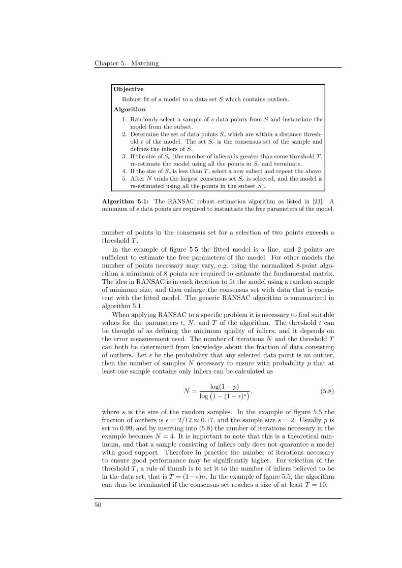
Chapter 5. Matching

Objective

Robust fit of a model to a data set S which contains outliers.

Algorithm

1. Randomly select a sample of s data points from S and instantiate themodel from the subset.

2. Determine the set of data points Sc which are within a distance thresh-old t of the model. The set Sc is the consensus set of the sample anddefines the inliers of S.

3. If the size of Sc (the number of inliers) is greater than some threshold T ,re-estimate the model using all the points in Sc and terminate.

4. If the size of Sc is less than T , select a new subset and repeat the above.5. After N trials the largest consensus set Sc is selected, and the model is

re-estimated using all the points in the subset Sc.

Algorithm 5.1: The RANSAC robust estimation algorithm as listed in [23]. Aminimum of s data points are required to instantiate the free parameters of the model.

number of points in the consensus set for a selection of two points exceeds athreshold T .

In the example of figure 5.5 the fitted model is a line, and 2 points aresufficient to estimate the free parameters of the model. For other models thenumber of points necessary may vary, e.g. using the normalized 8-point algo-rithm a minimum of 8 points are required to estimate the fundamental matrix.The idea in RANSAC is in each iteration to fit the model using a random sampleof minimum size, and then enlarge the consensus set with data that is consis-tent with the fitted model. The generic RANSAC algorithm is summarized inalgorithm 5.1.

When applying RANSAC to a specific problem it is necessary to find suitablevalues for the parameters t, N , and T of the algorithm. The threshold t canbe thought of as defining the minimum quality of inliers, and it depends onthe error measurement used. The number of iterations N and the threshold Tcan both be determined from knowledge about the fraction of data consistingof outliers. Let ǫ be the probability that any selected data point is an outlier,then the number of samples N necessary to ensure with probability p that atleast one sample contains only inliers can be calculated as

N =log(1 − p)

log(

1 − (1 − ǫ)s) , (5.8)

where s is the size of the random samples. In the example of figure 5.5 thefraction of outliers is ǫ = 2/12 ≈ 0.17, and the sample size s = 2. Usually p isset to 0.99, and by inserting into (5.8) the number of iterations necessary in theexample becomes N = 4. It is important to note that this is a theoretical min-imum, and that a sample consisting of inliers only does not quarantee a modelwith good support. Therefore in practice the number of iterations necessaryto ensure good performance may be significantly higher. For selection of thethreshold T , a rule of thumb is to set it to the number of inliers believed to bein the data set, that is T = (1− ǫ)n. In the example of figure 5.5, the algorithmcan thus be terminated if the consensus set reaches a size of at least T = 10.

50


5.3.3 Robust Estimation

Having introduced the normalized 8-point algorithm and the general RANSACalgorithm in the previous sections, in this section a method for identifying arobust set of keypoint inliers and computing the corresponding fundamentalmatrix using these algorithms in combination is developed.

The overall approach is to use the RANSAC algorithm outlined in algo-rithm 5.1. The model to fit in this case is the epipolar constraint given in (5.1),and estimation of the model parameters, i.e. the fundamental matrix, is doneusing the normalized 8-point algorithm. Let xi and x′

i denote the keypointlocations in the first and second image for the ith pair of matching keypointsfound during the keypoint matching step treated in section 5.2. The data set S,for which a robust model fit is sought, is then the set of corresponding keypointlocations. At least 8 corresponding points from this set are necessary for instan-tiating the model, but in this project random samples of size s = 12 are usedbased on the discussion in the following section.

For each iteration of the algorithm, a random sample of 12 point correspon-dences xi and x′

i is selected from S, and a corresponding fundamental matrix Fis estimated as described in section 5.3.1. Then the consensus set Sc is deter-mined as the subset of point correspondences in S for which some error measureis below a threshold t. Here a first-order approximation to the geometric re-projection error of the points, referred to as the Sampson distance [23], is used.For corresponding points xi and x′

i and fundamental matrix F, the Sampsondistance d⊥ can be computed from

d2⊥ =

(x′iTFxi)

2

(Fxi)21 + (Fxi)22 + (FTx′i)

21 + (FTx′

i)22

, (5.9)

where (Fxi)2k represents the square of the kth entry of the vector Fxi. Thus

point correspondences for which d⊥ < t are included in the consensus set. Thevalue of t is discussed in the following section.

For simplicity, a fixed number of iterations is used in this project, and thevalue of N is discussed in the following section. After the N iterations arecompleted, the largest consensus set Sc is selected, and the final fundamentalmatrix F is estimated from this set. To check whether an acceptable matchbetween the pair of input images has been found, the number of keypoint inliersis compared to a threshold M . If the number of inliers is less than M , thispair of input images is not an acceptable match, and further processing is notperformed for this pair. In this project the value M = 100 is selected to limitprocessing in later steps of reconstruction, and to prevent bad matching pairsfrom affecting performance during clustering.

For efficient implementation the normalization step described in section 5.3.1is performed before applying RANSAC as described above, and therefore thedata set S actually consists of the normalized point correspondences xi and x′

i,cf. section 5.3.1. A summary of the complete method developed in this sectionis given in algorithm 5.2.

5.3.4 Evaluation

In figure 5.6 the result of applying the above robust method to the same pairof input images as in figure 5.3 is shown. Comparing the figures, it is seen

51

Chapter 5. Matching

Objective

Given a set of matching keypoint locations xi and x′

i, determine a robustset of keypoint inliers and the corresponding fundamental matrix F.

Algorithm

1. Normalization: Let S be the set of transformed point correspon-dences xi = Txi and x′

i = T′x′

i, cf. section 5.3.1.2. Robust Estimation: Repeat for N iterations:

(a) Select a random sample of 12 correspondences from S and estimatethe corresponding fundamental matrix F′, cf. section 5.3.1.

(b) For all correspondences in S compute the Sampson distance d⊥

given F′ using (5.9).(c) Determine the consensus set Sc consisting of the correspondences

in S for which d⊥ < t.

Select the largest found consensus set Sc as the set of keypoint inliers,and re-estimate F′ from all correspondences in Sc.

3. Denormalization: Set the final fundamental matrix F = T′TF′T.

An acceptable match between the two input images has been found if thenumber of keypoint inliers is at least M .

Algorithm 5.2: Robust estimation of the fundamental matrix and identification ofkeypoint inliers using RANSAC and the normalized 8-point algorithm.

that most of the false matches are discarded as outliers. This image pair has1527 keypoint matches, and 1508 of these are now identified as keypoint inliers.There may be a few remaining false matches that by chance satisfy the epipolarconstraint, but their influence on the results is negligible.

The following is a discussion of the parameters selected for robust estima-tion of the fundamental matrix. Although 8 correspondences are sufficient forcomputing a fundamental matrix, a sample size s = 12 is chosen. The reasoningis that an initial least-squares fit from 12 true inliers increases the probabil-ity of other true inliers being within the distance threshold, and thus a largerconsensus set can be obtained.

The distance threshold t is set to the value 0.01, and this is the maximumSampson distance allowed for inliers. Note however that this threshold is appliedto normalized image coordinates, cf. algorithm 5.2, and therefore the value doesnot directly correspond to a pixel distance. In the images of figure 5.6 an averagescale of 0.0065 was applied during normalization, and thus t = 0.01 correspondsto a maximum reprojection error of approximately 1.5 pixels. For the inliers ofthis image pair the actual RMS reprojection error is 0.16 pixels, which is verygood compared to the distance threshold. For all matching image pairs in thedata sets the RMS reprojection error of inliers is less than 1 pixel.

The number of iterations is fixed to the value N = 500, even though lessiterations are sufficient for most image pairs in the data sets. Here this is com-pared to the theoretical number given by (5.8) in section 5.3.2. First the ratio ofinliers to matches, which gives an approximate probability of a correspondencebeing an inlier, is determined, and from this a suitable ǫ can be chosen. For allmatching image pairs in the data sets, the average number of keypoint matchesis 455, and on average there are 441 keypoint inliers. This gives a ratio of 0.97

52

5.4. Recovery of Relative Pose

200 400 600 800 1000 1200

200

400

600

800

(a)

200 400 600 800 1000 1200

200

400

600

800

(b)

Figure 5.6: Keypoint inliers for the two images shown in (a) and (b). Dots representthe location of keypoints in the image shown, and the other end of the lines indicate thelocation of the corresponding keypoints in the other image (only 25% of the 1508 inliersare shown).

0 500 1000 1500 2000 25000

500

1000

1500

2000

2500

Keypoint matches

Key

poin

t inl

iers

Figure 5.7: Number of keypoint matches and inliers for all matching pairs of inputimages in the data sets used in this project. The ratio of inliers to matches is computedas 0.98 using linear regression.

inliers per match. Employing linear regression as illustrated in figure 5.7 givesa ratio of 0.98 inliers per match. As can be seen from this figure, the number ofinliers is very close to being a linear function of matches, and this testifies thatthe quality of the SIFT keypoints is high. From the above a conservative guessis ǫ = 0.05, and inserting this into (5.8) in theory 6 iterations are sufficient.In other words, using 500 iterations ensures that around 83 random samplescontain only inliers, and of these samples the one with the highest number ofinliers is used for estimating the fundamental matrix.

5.4 Recovery of Relative Pose

From the estimated fundamental matrix it is possible to recover the relativepose of the two cameras. This involves computing a matrix referred to as theessential matrix, and this is treated in the following section. Then from theessential matrix, the relative pose between the cameras can be recovered, andthis process is explained in section 5.4.2.

53

Chapter 5. Matching

5.4.1 Computing the Essential Matrix

The first step of recovering the relative pose of the two cameras is to computethe essential matrix. The essential matrix E is a 3×3 matrix similar to the fun-damental matrix F, but it applies to cameras with known intrinsic calibration.Therefore this step depends on the intrinsic calibration of the images obtainedin the preprocessing step as described in section 4.2.

Recall from section 4.1 that a camera matrix is defined as P = K[R t], andlet x = PX be a point in the image. Knowing the camera calibration matrix Kfrom preprocessing, its inverse can be applied to the point x to obtain thepoint x = K−1x, which is expressed in normalized coordinates2. This removesthe effect of the intrinsic parameters as can be seen from x = [R t]X. Acamera matrix of the form K−1P = [R t] is referred to as a normalized cameramatrix [23].

In the following two normalized camera matrices P = [I 0] and P′ = [R t]corresponding to the first and second image respectively in a pair of input imagesare considered. The corresponding camera calibration matrices K and K′ areknown from preprocessing, and thus for corresponding points x and x′ thenormalized points x = K−1x and x′ = K′−1x′ can be computed. The essentialmatrix E is now defined by

x′TEx = 0. (5.10)

Comparing this to (5.1) it is seen that the essential matrix is the fundamentalmatrix for normalized cameras. From above it can be derived that

E = K′TFK. (5.11)

The fact that the cameras are normalized imposes additional constraintson the essential matrix. For an essential matrix to be valid, it must have twosingular values that are equal, and one that is zero [23]. For an essential matrix Ecomputed using (5.11), this constraint can be enforced in a way similar to thesingularity constraint for the fundamental matrix as explained in section 5.3.1.Employing SVD let E = UDVT, with D = diag(r, s, t) satisfying r ≥ s ≥ t.Then the constraint can be enforced by computing u = (r + s)/2 and settingthe final essential matrix E = Udiag(u, u, 0)VT.

5.4.2 Relative Pose from the Essential Matrix

From the essential matrix E computed using the above method, the relativepose between the two cameras can be recovered up to an unknown scale. Withthe normalized camera matrices P = [I 0] and P′ = [R t], the relative pose isdefined by the rotation matrix R and the translation vector t. The following isbased on [23] and [31].

Disregarding the unknown scale, the SVD of the essential matrix can bewritten as E = Udiag(1, 1, 0)VT, with U and V chosen such that det(U) > 0and det(V) > 0. Then the translation vector t equals either +u3 or −u3, andthus ||t|| = 1. By introducing the matrix

W =

0 1 0−1 0 00 0 1

, (5.12)

2Note that this normalization is not the same as in the normalized 8-point algorithm.

54

5.4. Recovery of Relative Pose

AB

AB /A B /

A B

(a) (b)

(c) (d)

Figure 5.8: Geometrical illustration of the four possible camera configurations [23].Between left and right the baseline is reversed. Between top and bottom rows thecamera B rotates 180◦ about the baseline. Only in configuration (a) the triangulatedpoint is in front of both cameras.

the rotation matrix R is equal to either Ra = UWVT or Rb = UWTVT. Thisleads to 4 possible solutions for P′ given by

P′A = [Ra u3], P′

B = [Ra − u3],

P′C = [Rb u3], and P′

D = [Rb − u3]. (5.13)

Only one of these correspond to the true configuration, and to determine whichone, the chirality constraint is imposed. By triangulating3 a space point X fromtwo corresponding points in the images using the camera matrices P and P′

A

the ambiguity can be resolved. The four solutions are illustrated in figure 5.8.As can be seen from the figure, the triangulated point is only in front of bothcameras in one of the configurations.

Let X = [X1 X2 X3 X4]T be the homogeneous 4-vector representing the

triangulated point, and compute c1 = X3X4 and c2 = (P′AX)3X4. Then if

c1 > 0 the point is in front of the first camera, and if c2 > 0 the point is in frontof the second camera. Hence if both c1 > 0 and c2 > 0 the true configurationis P′ = P′

A. If c1 < 0 and c2 < 0 the baseline is reversed and P′ = P′B.

On the other hand if c1c2 < 0 it is necessary to check the twisted pair, socompute c3 = (P′

CX)3X4. Then if c1 > 0 and c3 > 0 the true configurationis P′ = P′

C . Finally, if c1 < 0 and c3 < 0 the baseline is reversed and P′ = P′D.

5.4.3 Evaluation

One point correspondence is sufficient to determine the correct camera configu-ration using the chirality constraint. Such point correspondence is convenientlyobtained from the locations of a keypoint inlier in the two images.

3Triangulation is treated in section 6.1.1.

55

Chapter 5. Matching

Figure 5.9: Example of the relative pose recovered for a pair of input images. Inaddition to the cameras, triangulated keypoint inliers are shown as green dots.

It was discovered, however, that in practice it is not enough to use a singlekeypoint correspondence. As discussed in section 5.3.4, some false matches mayby chance satisfy the epipolar constraint and are thus wrongly identified askeypoint inliers. When triangulating these false matches, the resulting pointmay end up behind the cameras, and therefore the camera configuration ischecked for all keypoint inliers. The most frequent configuration is deemedcorrect, and any mismatching points are discarded as outliers. For instance inthe image pair shown in figure 5.6, four keypoint inliers were discarded becausethey did not match the configuration of the majority of correspondences.

In figure 5.9 an example of recovering the relative pose of two cameras usingthis method is shown. In addition to the two cameras, also the triangulatedkeypoint inliers are shown.

5.5 Conclusion

In this chapter, the matching step of the proposed reconstruction method hasbeen treated in detail, and a robust method for estimating the relative posein all matching pairs of input images has been developed. Epipolar geometryand the fundamental matrix were introduced in section 5.1, and in section 5.2a method for establishing an initial correspondence between keypoints in a pairof input images was developed. Then in section 5.3, a robust method for iden-tifying a set of keypoint inliers and estimating the fundamental matrix, basedon a combination of RANSAC and the normalized 8-point algorithm, was de-veloped. Finally in section 5.4 a method for extracting the relative pose of thetwo cameras in a pair of input images was described. A lot of ground has beencovered in this chapter, and this provides the basis for recovering structure andmotion in the clustering step, which is the topic of the following chapter.

56

Chapter 6

Clustering

In this chapter, the clustering step of the proposed reconstruction method isdocumented. The purpose is to recover structure and motion for all inputimages. That is the positions of keypoints in space and the extrinsic parametersfor all input images are estimated, yielding a result as illustrated in figure 3.2.In this context a cluster is a collection of cameras with estimated extrinsicparameters and a point cloud of estimated keypoint positions. The developedmethod builds on the the recovered relative pose and the set of keypoint inliersidentified for each matching pair of input images in the previous step.

Traditionally methods for recovering structure and motion are based on find-ing a global initial guess for the extrinsic parameters of all cameras and all pointpositions, and then performing a final optimization using bundle adjustment.For bundle adjustment to succeed, a good initial guess of the global structureand motion is necessary [37]. In this project a bottom up approach, in whichbundle adjustment is applied throughout the clustering process, has been de-veloped. This minimizes the risk that a bad initial guess prevents successfulrecovery of structure and motion. A convenient consequence of applying bun-dle adjustment this way is that simpler and less accurate methods for initialestimation can be employed without affecting the end result.

The overall approach of the developed clustering method is to initialize thecluster from the best matching image pair, and then add images to the clusteriteratively until all input images are included. When adding an image to thecluster, the relative pose recovered in the matching step is used for computingan initial estimate of the extrinsic camera parameters, and keypoint inliers aretriangulated to obtain an estimate of keypoint positions. Each time an imagehas been added to the cluster, the recovered structure and motion is optimizedby applying bundle adjustment.

In the following sections the details of the developed clustering method aredocumented. In section 6.1 the process of adding the first pair of images tothe cluster is treated. This corresponds to reconstruction from stereo imagesand includes triangulation of keypoints. Section 6.2 then covers addition ofa third image to the cluster. Having introduced these two basic steps, thedeveloped clustering algorithm itself is treated in section 6.3. For each iterationof clustering an optimization step, consisting of bundle adjustment and variousrobustness measures, is applied. Section 6.4 provides an overview of bundleadjustment, and finally in section 6.5 the optimization step is treated.

57

Chapter 6. Clustering

6.1 The First Pair of Images

In this section, the first step of clustering is treated, namely initializing thecluster from the best matching image pair found during the matching step.This pair is simply the pair of input images having the largest set of keypointinliers. Let m be the number of input images. Then the best matching pairconsists of images (a, b), for some a and b satisfying 1 ≤ a < b ≤ m.

Now let P(a,b) denote the relative pose recovered for this pair. This is a nor-malized camera matrix composed of a rotation and a translation as discussed insection 5.4.2. This directly leads to an initial estimate of the extrinsic param-eters for the cameras corresponding to images a and b. The cluster is simplyinitialized using the two camera matrices Pa = [I 0] and Pb = P(a,b).

The relative pose can only be recovered up to an unknown scale, and thislimitation also applies to the structure and motion recovered during clustering.By selecting the identity matrix for Pa, the world coordinate system is definedby the camera of image a, and thus structure and motion is only recovered upto an arbitrary similarity transform.

6.1.1 Triangulation of Keypoints

With two cameras in the cluster, the positions of the keypoint inliers of theimage pair are estimated using triangulation. As discussed in the chapter in-troduction, bundle adjustment is applied in each iteration of clustering, andtherefore a simple method can be used for triangulation. Here the linear trian-gulation method described in [23] is used. In the following the generic methodis described, and then it is applied to the problem of triangulating the keypointinliers of the image pair.

Given measured corresponding points x and x′ in a pair of images withcamera matrices P and P′, the objective of triangulation is to estimate thespace point X. Under ideal circumstances x = PX and x′ = P′X, but due tonoise in the image points an exact solution can not be found, see figure 6.1.As these equations involve homogeneous vectors, the relation is rather x ∝ PX,and likewise for the second image. That is, vectors x and PX are not necessarilyequal but have the same direction and may differ in magnitude by a non-zeroscale factor. Employing the Direct Linear Transformation (DLT) algorithm [23],the triangulation problem can be expressed in the form AX = 0, which is anequation linear in X.

The unknown homogeneous scale factor can be eliminated by utilizing thattwo non-zero vectors a and b are parallel if and only if a×b = 0. Then for thefirst image x × (PX) = 0. Introducing the notation a × b = [a]×b, where [a]×is the skew-symmetric matrix

[a]× =

0 −a3 a2

a3 0 −a1

−a2 a1 0

, (6.1)

this can be written [x]×(PX) = 0. Letting x = [x y 1]T and writing out gives

0 −1 y1 0 −x−y x 0

p1TXp2TXp3TX

= 0, (6.2)

58

6.1. The First Pair of Images

x

/

x /

C C

(a)

xx

e

/

e /

l = F /x /l = F x

image 1 image 2

(b)

Figure 6.1: The effect of imperfectly measured points [23]. a) The rays back-projected from measured points x and x′ are skew in general. b) The measured pointsdo not satisfy the epipolar constraint. The epipolar line l is the image of the raythrough x′, and l′ is the image of the ray through x. Since the rays do not intersect,x does not lie on l, and x′ does not lie on l′.

where piT are the rows of P. This leads to three equations

x(p3TX) − (p1TX) = 0 (6.3)

y(p3TX) − (p2TX) = 0 (6.4)

x(p2TX) − y(p1TX) = 0 (6.5)

of which two are linearly independent.By including two equations for each image, a set of four equations with four

unknowns is obtained in the form AX = 0, with A being the 4 × 4 matrix

A =

xp3T − p1T

yp3T − p2T

x′p3T − p′1T

y′p3T − p′2T

. (6.6)

The solution is only determined up to scale, so the additional constraint ||X|| = 1is added. This system can be solved using the SVD, as previously discussed, byletting A = UDVT. Then the solution is the last column of V, i.e. the estimatedposition of the space point X = v4.

Returning to the problem of triangulating the keypoint inliers for the imagepair (a, b) in the cluster, the goal is to obtain a set of space points Xi, which aretriangulated from the locations of the keypoint inliers. Denote by xi,a and xi,b

the locations expressed in normalized coordinates of keypoint i in image a and brespectively. To obtain normalized coordinates, the inverse camera calibration

59


matrices K−1a and K−1

b corresponding to the images are applied to the keypointlocations. The space points Xi are then triangulated using the above methodfor corresponding points xi,a and xi,b, and camera matrices Pa and Pb.

The triangulated points are added to the cluster, which now consists of twocameras defined by the camera matrices Pj , j ∈ {a, b}, and the set of points Xi

triangulated from the keypoint inliers of the image pair. The final step of clusterinitialization is to perform optimization of the recovered structure and motionas explained in section 6.5. The method for cluster initialization covered hereis evaluated in section 6.2.4 below.

6.2 Adding a Third Image

With the cluster consisting of two cameras and points triangulated from thekeypoint inliers of the corresponding image pair, the next task of clustering isto augment the cluster with another image. The image selected for additionto the cluster is the image c satisfying 1 ≤ c ≤ m and c /∈ {a, b}, which hasmost keypoint inliers with any of the images already in the cluster. That is,image c is part of a matching image pair that also contains either image aor b and thus is a neighbour of the cluster. In the following assume that thisimage pair is (b, c) where b < c. Augmenting the cluster consists of threemain steps, namely obtaining an initial pose estimate with unknown scale forthe new camera, recovering the relative scale, and triangulating new keypointinliers. These steps are explained in the following sections.

6.2.1 Initial Pose Estimate

From matching the estimated relative pose P(b,c) between image b and c isknown. An initial pose estimate for the camera corresponding to image c canbe obtained up to scale by combining this information with the current state ofthe cluster. The extrinsic parameters for the camera corresponding to image bare defined by Pb, which is part of the cluster. With P(b,c) = [R(b,c) t(b,c)]and Pb = [Rb tb], the initial estimate is obtained by computing

[

Rc tc

1

]

=

[

R(b,c) t(b,c)

1

] [

Rb tb

1

]

(6.7)

and letting Pc = [Rc tc], where the hat indicates the unknown relative scale.In the case where c < b, the relative pose recovered during matching would

instead be P(c,b). This is the inverse Euclidean transformation of P(b,c), so it isnecessary to first compute

P(b,c) =[

RT(c,b) −RT

(c,b)t(c,b)

]

, (6.8)

and then the initial pose estimate Pc can be found using (6.7).

6.2.2 Recovering the Relative Scale

The relative poses recovered during matching all have a unit translation vector,and therefore the distance between the cameras defined by Pa and Pb is 1. This

60

6.2. Adding a Third Image

a b

c

11

(a)

a b

c

1

s

(b)

Figure 6.2: Illustration of the relative scale of distances between cameras a, b, and c

in the cluster. a) The initial pose estimate for camera c with unknown scale. b) Thepose estimate for camera c after the relative scale has been recovered.

X1 X2

x1,b x2,bx1,c

x2,c

b c1

d

(a)

X1 X2

x1,b x2,bx1,c

x2,c

b cs

s · d

(b)

Figure 6.3: The true distance between two cameras can not be determined given pointcorrespondences alone. Two space points X1 and X2 are observed by cameras b and c.The focal length and image plane dimensions are the same in both figure (a) and (b),and as can be seen the scale s has no influence on the position of the projections x1,b,x2,b, x1,c, and x2,c.

is also the case for the cameras defined by Pb and Pc, but the true distancesbetween the cameras in image pairs (a, b) and (b, c) are unlikely to be identical.Therefore it is necessary to recover the relative scale by computing a scalefactor s, which puts camera c in the correct position relative to the cluster, seefigure 6.2. The problem arises because the true distance between two camerascan not be determined from a set of corresponding points in the images asillustrated in figure 6.3. Fortunately it is possible to recover the relative scale ifat least one point is observed in all three images [37].

Suppose that a keypoint inlier in image pair (a, b) and a keypoint inlierin image pair (b, c) share a common keypoint in image b, then this keypoint isobserved in all three images. Let Xi be the position of this keypoint triangulatedusing the keypoint locations xi,a and xi,b and camera matrices Pa and Pb as

explained in section 6.1.1. Another space point Xi can now be triangulatedusing the keypoint locations xi,b and xi,c in image pair (b, c) and the camera

matrices Pb and Pc. It is known that Xi and Xi represent the same point in thescene, but due to the unknown scale the triangulated position of these pointsmay differ as illustrated in figure 6.4a.

61


Xi

Xi

Ca Cb

11

Cc

(a)

Xi

Ca Cb1

s

Cc

(b)

Figure 6.4: Recovering the relative scale using two space points Xi and Xi triangu-lated using camera matrices (Pa, Pb) and (Pb, Pc) respectively. The triangle formedby Xi, Cb and Cc in figure (a) is similar to the triangle formed by Xi, Cb, and Cc infigure (b), and thus the relative scale s can be recovered.

The figure hints how the relative scale may be recovered. The triangle formedby Xi, and the camera centres Cb and Cc is similar to the triangle in figure 6.4bformed by Xi, Cb, and Cc. Therefore the relative scale can be computed as

s =||Xi − Cb||||Xi − Cb||

, (6.9)

where the camera centres Cb and Cc are given by

Cb = −RTb tb, and (6.10)

Cc = −RTc tc. (6.11)

The pose estimate for camera c with correct relative scale can now be computedby first obtaining the corrected camera position as

Cc = Cb + s · (Cc − Cb), (6.12)

and then computing tc = −RcCc. Finally the corrected pose estimate be-comes Pc = [Rc tc].

Typically there is more than one keypoint that is observed in all three images,and a better estimate of the relative scale s can be obtained by utilizing allcommon keypoints. A simple average of relative scales computed using theabove method for all common keypoints suffices, because gross outliers havebeen discarded in previous steps and bundle adjustment is applied afterwards.When the extrinsic parameters for camera c have been recovered, the cameramatrix Pc is added to the cluster.

6.2.3 Triangulation of New Keypoints

When recovering the relative scale as described in the previous section, a setof keypoints that are observed in all three images is identified. The spacepoints Xi corresponding to these keypoints are already triangulated using theprojections xi,a and xi,b from image pair (a, b) as explained in section 6.1.1, andthey are part of the cluster. However, the purpose of bundle adjustment is tooptimize structure and motion using observations from all images, and therefore

62

6.2. Adding a Third Image

(a) (b)

Figure 6.5: Example of structure and motion recovered during the first two steps ofclustering. a) After initialization, the cluster consists of two cameras and 1771 key-points triangulated from the corresponding image pair. b) Adding another imageresults in a third camera and additional triangulated keypoints, leading to a total of2837 keypoints.

the common keypoints Xi are updated with the additional observations xi,c inimage c. I.e. the cluster now contains a set of points Xi which are observed onlyin image pair (a, b), and another set of points Xi which are observed in bothimage pairs (a, b) and (b, c).

When adding the third image, new keypoints that are observed in imagepair (b, c) but not in (a, b) may be present. These keypoints should also be tri-angulated and added to the cluster. Therefore new space points Xi representingthese keypoints are triangulated using corresponding points xi,b and xi,c andcamera matrices Pb and Pc.

In summary, after adding image c the cluster contains three cameras definedby the camera matrices Pj , j ∈ {a, b, c}, and the set of points Xi with corre-sponding projections xi,j in two or three of the images a, b, and c. As in clusterinitialization, the final step of augmenting the cluster is to perform optimizationas explained in section 6.5. The process outlined here is the general method foradding an image to the cluster.

6.2.4 Evaluation

In this section examples of results obtained using the two basic steps of clus-tering treated above, namely initialization of the cluster and augmenting thecluster with a third image, are shown. In figure 6.5a an example of structureand motion recovered using the method for cluster initialization covered in sec-tion 6.1 is shown. In this example the best matching image pair is (3,4) whichhas 1771 keypoint inliers.

The result of adding a third image to the cluster is shown in figure 6.5b. Inthis example, the image pair with most keypoint inliers that also contains eitherimage 3 or 4 is image pair (4, 5) with 1504 inliers. An initial pose estimate forcamera 5 is computed, and a set of 438 keypoints that are observed in all threeimages is identified. Using the common keypoints, the relative scale is estimatedto be 1.05, and a corrected pose estimate for camera 5 is computed. Finally theremaining 1066 keypoint inliers of image pair (4, 5) are triangulated and addedto the cluster, and the cluster is optimized.

63


6.3 The Clustering Algorithm

With the two basic steps of clustering covered in the previous sections, in thissection the developed clustering algorithm itself is documented. An importantfactor driving the development of the clustering algorithm is that it shouldmake effective use of the available data, and preserve as much information aspossible. That is, the algorithm should strive to obtain a maximum number ofstable keypoints, but without introducing bad measurements. Having a largenumber of triangulated points with correct projections in the images of thecluster improves the quality of the recovered structure and motion, becausemore information is available for bundle adjustment in the optimization step.

To obtain the maximum number of keypoints, a good strategy is to buildthe cluster using the matching image pairs with most keypoint inliers. Thisapproach was taken in the first two steps of clustering explained in sections 6.1and 6.2, and it can be applied each time an image is added to the cluster.The strategy is analogous to finding a maximum spanning tree in a connectedgraph formed by vertices representing the input images and edges representingmatching pairs of input images. In the following section an introduction to theconcept of maximum spanning trees is given, and then in section 6.3.2 this isapplied to the problem of clustering.

6.3.1 Maximum Spanning Trees

A connected, undirected graph is given by G = (V, E), where V is a set ofvertices, and E is a set of edges representing possible connections between thevertices. For each edge (u, v) ∈ E there is an associated weight w(u, v) specifyingthe cost of connecting the vertices u and v using this edge. In many applicationsan acyclic subset T ⊆ E that connects all the vertices, and which minimizes thetotal weight

w(T ) =∑

(u,v)∈T

w(u, v) (6.13)

is sought. In this situation T represents a tree which is referred to as a minimumspanning tree [18]. In the same way a maximum spanning tree can be found asan acyclic subset T ⊆ E that maximizes the total weight in (6.13).

A simple algorithm for finding minimum spanning trees is Prim’s algorithm,which is easily adapted to the problem of finding a maximum spanning tree.The algorithm is greedy in the sense that it always makes the choice that isbest at the moment. This strategy is not generally guaranteed to find globallyoptimal solutions, but for this problem an optimal solution is obtained [18].

The overall idea of Prim’s algorithm is explained in the following, whereit has been adapted to finding a maximum spanning tree. The algorithm isinitialized by letting T = ∅. Then as long as T does not form a tree spanningall vertices V , find a safe edge (u, v) ∈ (E − T ) and add it to T . A safe edgeis an edge that has maximum weight and connects an isolated vertex in thegraph GT = (V, T ) to the tree T . For the first step, an edge (u, v) ∈ E withmaximum weight can be selected as a safe edge. Upon termination, the set ofedges in T define a maximum spanning tree of the graph G.

64

6.3. The Clustering Algorithm

Figure 6.6: The graph G = (V, E) representing a data set consisting of 10 images.The vertices V = {0, . . . , 9} represent the input images, while the edges (u, v) ∈ E

represent matching image pairs. The weight w(u, v) of an edge is the number ofkeypoint inliers for image pair (u, v).

6.3.2 Building the Cluster

Based on the above clustering can be seen as the task of finding a maximumspanning tree of a graph G = (V, E), where V is the set of input images, E isthe set of matching image pairs (u, v) found in the matching step, and theweight w(u, v) of each edge is the number of keypoint inliers for the imagepair (u, v). During the process, camera matrices Pj corresponding to the inputimages and space points Xi corresponding to the keypoints of the images arerecovered. In figure 6.6 the graph G is shown for a data set consisting of 10 im-ages. This data set, which was also used for the examples of recovered structureand motion in figure 6.5, is used for illustration throughout the explanation ofthe clustering algorithm below.

For efficient implementation, two distinct sets of edges are maintained in theclustering algorithm: a set of free edges F containing all matching image pairsthat are not yet part of the cluster, and a set of open edges O containing allmatching image pairs which have one image in the cluster. In the following thetwo main steps of the algorithm, initialization of the cluster and augmentingthe cluster, are treated.

Cluster Initialization First all matching image pairs are added to the setof free edges by letting F = E and the set of open edges O = ∅. Then thefree edge (a, b) ∈ F which has maximum weight is selected as the first edge ofthe spanning tree, and this edge is removed from F . The selected edge (a, b)corresponds to the best matching image pair, and it is added to the cluster usingthe method of section 6.1. Now the cluster consists of two cameras definedby Pj , j ∈ {a, b} and a set of triangulated keypoints Xi with correspondingprojections xi,j . As a final step of initialization all matching image pairs thatare connected to either image a or b are moved from the set of free edges F intothe set of open edges O.

In figure 6.7a a graph illustrating the result of this process is shown, whereimages from the best matching image pair (3,4) are included in the cluster. Ascan be seen from the figure, six edges are moved to the set of open edges, andimages 2, 5 and 6 are candidates for being added to the cluster next.

Augmenting the Cluster In this step the maximum spanning tree is grown,and it is repeated until all input images are part of the cluster. The openedge (b, c) ∈ O with maximum weight is selected for augmenting the cluster, and

65


it is removed from O. Suppose that image b is already part of the cluster, thenimage c is being added. The edge (b, c) is a strong edge, because it representsthe matching image pair with most keypoint inliers that connects image c to thecluster. There may be other open edges in O connecting image c to the cluster,but they have less keypoint inliers and are thus weak edges.

The new image c is added to the cluster via the strong edge representing im-age pair (b, c) using the method of section 6.2. In this process the new cameradefined by Pc is added to the cluster, any keypoints Xi already in the cluster thatare also inliers of image pair (b, c) are updated with projections xi,c for bundleadjustment, and the remaining keypoint inliers of image pair (b, c) are trian-gulated from corresponding projections xi,b and xi,c yielding new keypoints Xi

which are added to the cluster.Any weak edges connecting image c to the cluster are now also removed from

the set of open edges O, but see below for how weak edges are utilized. Afterimage c has been added to the cluster, all free edges representing image pairsconnected to that image are moved from the set F into the set of open edges O.As long as open edges remain, the cluster is augmented using this method.

Continuing the example from above, a graph illustrating the result of aug-menting the cluster with a third image is shown in figure 6.7b. The openedge (4, 5) is selected as the strong edge connecting image 5 to the cluster,but there is also a weak edge (3, 5) which has less keypoint inliers, see below.After image 5 has been added to the cluster, the two edges (2, 5) and (5, 6) aremoved to the set of open edges, and image 2 and 6 are candidates for beingadded to the cluster next.

Utilizing Weak Edges As discussed above, the clustering algorithm shouldstrive to obtain a maximum number of stable keypoints, but without introducingbad measurements. One way to improve stability of keypoints is to add projec-tions from more images when available, but this only helps if the projectionsadded are actually correct.

Consider a cluster initialized from the matching image pair (a, b), which isaugmented with a new image c via the strong edge (b, c). Now suppose thatthere is a weak edge (a, c) that also connects image c to the cluster. Thenthe keypoint inliers of image pair (a, c) are likely to be correct, and can thusbe utilized for updating the keypoints that are already triangulated with moreprojections for bundle adjustment. To avoid introducing bad measurements,however, no new keypoints are triangulated from weak edges.

Experiments have shown that for most data sets, simply adding projectionsfrom all weak edges may lead to introduction of bad measurements. Thereforea parameter W is defined, which limits the number of weak edges that maybe utilized when augmenting the cluster with a new image. Then at most thebest W weak edges are utilized. The value of W is discussed in the followingsection.

Continuing the example from above, figure 6.7c shows the graph resultingfrom augmenting the cluster with image 6 via the strong edge (5, 6) and utilizingweak edges (4, 6) and (3, 6). The previously free edge (6, 7) is now moved to theset of open edges. Figure 6.7d shows one more iteration, and in figure 6.7e thecomplete graph obtained from clustering this data set is shown. As can be seenin the last figure, the strong edges form a maximum spanning tree of the original

66

6.3. The Clustering Algorithm

(a)

(b)

(c)

(d)

(e)

Figure 6.7: Graphs illustrating the progress during clustering for a data set. Verticesmarked in black represent images in the cluster, and vertices filled with gray representcandidate images for being added to the cluster next. Figure (a) shows the state aftercluster initialization, and figures (b)–(d) show how the cluster is augmented with moreimages. In figure (e) the final graph is shown, where the strong edges form a maximumspanning tree.

67


graph G = (V, E) shown in figure 6.6. The weak edges are the remaining edgesof the graph, but for other data sets some matching image pairs may be ignoredif they are not among the best weak edges in any iteration of the algorithm.

The clustering algorithm terminates when there are no more open edgesavailable in O, and the final result is the set of camera matrices Pj correspondingto all input images, and the set of space points Xi with associated keypointlocations xi,j in the input images.

6.3.3 Evaluation

The graphs in figure 6.7 illustrate the progress of clustering for one data set,but the resulting graph in figure 6.7e is representative for most of the data setsused in this project. From this graph it is seen that the strong edges connectthe input images in sequence. This is because the images in this data set werecaptured with movement primarily along one direction, but this is not requiredby the clustering algorithm. In fact the tree formed by the strong edges can beany kind of tree. In the figure it is also seen that weak edges typically connectimages close to each other in the sequence. This is also due to the way theimages of this data set are captured, and in general weak edges are most likelyto be present for images that are captured from similar perspectives.

For most data sets used in this project maximum of W = 2 weak edgesutilized when augmenting the cluster with an image works well, and addingprojections from the weak edges increases the number of stable keypoints ob-tained. But for one data set, using more than one weak edge leads to a significantdecrease in the number of keypoints obtained, and thus for this data set a valueof W = 1 was chosen. Evaluation of the structure and motion results obtainedusing the clustering algorithm treated here is postponed to section 6.5.1.

6.4 Bundle Adjustment

Each time the cluster is augmented with an image, bundle adjustment is appliedto the recovered structure and motion as part of an optimization step. Inthis section, an overview of bundle adjustment is given. For a more in-depthtreatment refer to [23] and [26].

Given a set of images depicting a number of 3D points from different view-points, bundle adjustment solves the problem of simultaneously refining thepositions of these points and the calibration parameters of the cameras that cap-tured the images, based on observed 2D projections of the points in the images.Bundle adjustment provides a statistically optimal solution to this problem, andunder the assumption that the error of observed projections is zero-mean Gaus-sian, bundle adjustment is the maximum likelihood estimator [26]. The namerefers to the bundles of light rays originating from each point in the scene andconverging in the optical centre of each camera, which are adjusted optimallywith respect to both structure and motion parameters.

Essentially bundle adjustment amounts to minimizing the reprojection errorbetween observed and predicted image points. This error is expressed as asum of squares of a large number of nonlinear, real-valued functions, and thusnonlinear least-squares algorithms are employed for minimization. For bundleadjustment the Levenberg-Marquardt algorithm is typically used, because it

68

6.4. Bundle Adjustment

has the ability of converging quickly while still being tolerant to a wide rangeof initial guesses [26].

More formally, the problem of bundle adjustment can be stated as follows.Assume that n points in 3-space are observed in m images, and denote by xi,j

the homogeneous 3-vector representing the observed projection of the ith pointon the jth image. Then bundle adjustment amounts to refining the m cameramatrices Pj and the n points represented by homogeneous 4-vectors Xi, suchthat the observed projection xi,j is closely approximated by the predicted pro-jection xi,j = PjXi. Here it is assumed that an initial estimate of the cameramatrices Pj and points Xi are available, as is the case when bundle adjustmentis used in combination with the clustering algorithm treated above.

Typically each 3D point i is observed only in a subset of the m images.Therefore let vi,j denote binary variables that equal 1 if point i is visible inimage j and 0 otherwise. Now by parameterizing each camera j by a vector aj

and each 3D point i by a vector bi as explained in the following section, bundleadjustment minimizes the reprojection error with respect to all 3D points andcamera parameters. Specifically

arg minaj ,bi

n∑

i=1

m∑

j=1

vi,j d(

Q(aj ,bi), xi,j

)2, (6.14)

where Q(aj ,bi) is the predicted projection xi,j of point i on image j, andd(x,y) denotes the Euclidean distance between image points represented bythe vectors x and y. From (6.14) it is clear that bundle adjustment minimizesa physically meaningful criterion, namely the geometric reprojection error, asopposed to algebraic approaches [26].

6.4.1 Sparse Bundle Adjustment

If bundle adjustment is implemented naively the complexity of the problem isvery large due to the high number of minimization parameters. In the case ofEuclidean reconstruction with intrinsically calibrated cameras as in this project,each 3D point gives rise to 3 parameters, and each camera gives rise to 6 param-eters as explained below. Thus the total number of minimization parametersbecomes 3n + 6m. For instance when applying bundle adjustment in the laststep of clustering for the data set illustrated by the graph in figure 6.7e, the min-imization involves 4426 points in 10 images leading to total of 13338 variables.Fortunately it is possible to take advantage of the fact that there is no inter-action among parameters for different 3D points and cameras. When solvingthe minimization problem of bundle adjustment, the normal equations involvedhave a sparse block structure due to this lack of interaction, and algorithms forsparse bundle adjustment taking advantage of this are available. In this projectSBA1, which is an open source library providing a C/C++ implementation ofgeneric sparse bundle adjustment [26], is used.

The algorithm implemented in the SBA library is generic in the sense thatcameras and points can be parameterized in different ways depending on thespecific problem at hand. As discussed above, in this project bundle adjust-ment is applied to the problem of Euclidean reconstruction with intrinsically

1http://www.ics.forth.gr/~lourakis/sba/

69


(a) (b)

Figure 6.8: Example of the inversion of camera and point positions that mighthappen during bundle adjustment. a) Correct structure and motion. b) The clusterhas been inverted, and points appear behind the cameras by which they are observed.

calibrated cameras. In this configuration the n 3D points are trivially repre-sented using 3-dimensional vectors bi. The m cameras, however, are definedby normalized camera matrices Pj . Instead of including all elements of thematrices Pj = [Rj tj ] in bundle adjustment, the cameras are parameterizedusing 6-dimensional vectors aj which capture the 6 degrees of freedom for eachcamera, i.e. 3 for rotation and 3 for translation. The results of applying bundleadjustment to the recovered structure and motion are evaluated in section 6.5.1.

6.5 Optimization and Robustness

In this final section on clustering, the optimization step that is applied eachtime an image has been added to the cluster is treated. The primary reasonsfor performing optimization throughout the clustering process are, as discussedin the chapter introduction, that this minimizes the risk of a bad initial guesspreventing recovery of structure and motion, and that simpler methods can beemployed without affecting the end result. But this strategy also leads to animprovement in the obtained structure and motion estimates.

Optimization is performed for the current state of the cluster, and the firststep is to apply bundle adjustment to the recovered structure and motion usingthe method described in the previous section. That is, the camera matrices Pj

and the points Xi currently in the cluster are updated with the statisticallyoptimal parameters given the observed projections xi,j .

As discussed in section 5.3.2 in general least-squares methods are sensitiveto outliers, and this also applies to the bundle adjustment method describedin the previous section. Although most keypoint outliers are discarded duringmatching, previously undetected outliers may manifest themselves during clus-tering. Therefore after bundle adjustment has been applied, any points thathave a maximum reprojection error above some threshold are removed from thecluster to improve robustness. This prevents these points from having negativeimpact during successive iterations of clustering. The value of the threshold andthe effect of pruning such points is discussed in the following section.

During development it was discovered, that on rare occasions the positionsof cameras and points in the cluster were inverted during bundle adjustment.The effect of this inversion is that all points suddenly appear behind the cameras

70

6.5. Optimization and Robustness

(a) (b)

Figure 6.9: Examples of the final recovered structure and motion for two data sets.a) Cluster consisting of 10 images and 4426 points. b) Cluster consisting of 10 imagesand 4087 points.

by which they are observed. This situation is illustrated in figure 6.8. Such in-version might happen, because the SBA library does not enforce the constraintthat observed points must be in front of cameras. Mathematically the inversesolution is equally good, but when augmenting the cluster with another im-age, this inversion causes problems and therefore it needs to be detected andcorrected for clustering to be robust.

The last task of the optimization step is to normalize the cluster, such thatthe distance between the cameras of the first image pair added to the cluster isequal to 1. This normalization is not strictly necessary, because the recoveredstructure and motion is always subject to an arbitrary similarity transform, butit makes the results of clustering more consistent.

In addition to the optimization and robustness measures discussed above,which are applied after augmenting the cluster, a couple of precautionary mea-sures are applied during clustering itself. Specifically, when triangulating newpoints, any points that end up behind the cameras by which they are observedare discarded. And when updating a point with additional projections, if it isdiscovered that the point matches different keypoints it is deemed a mismatch,and the point is discarded and any associated keypoints are excluded from fur-ther processing.

6.5.1 Evaluation

In figure 6.9 two examples of the final structure and motion recovered using theclustering method developed in this chapter are shown. Figure 6.9a shows thecluster corresponding to the graph in figure 6.7e, and in the following the resultsof clustering for this data set is used for discussion.

The cluster consists of 10 images and 4426 points with a total of 10196 ob-served projections, i.e. corresponding keypoint locations, in the images. Thuson average each stable keypoint has projections in 2.3 images, see the histogramin figure 6.10a. The RMS reprojection error for points in the cluster is 0.22 pix-els, which is very good. In figure 6.10b a histogram of the reprojection errorfor observed projections is shown, and as can be seen virtually all keypointshave reprojection errors below one pixel. This supports that the structure andmotion is recovered with high accuracy. In figure 6.11a a box plot of the re-projection errors for points in the cluster with different number of projections

71


2 3 4 5 60

1000

2000

3000

4000

Observed projections

Poi

nts

(a)

0 1 2 30

2000

4000

6000

8000

10000

Reprojection error [pixels]

Obs

erve

d pr

ojec

tions

(b)

Figure 6.10: a) Histogram of the number of projections for points in the cluster.b) Histogram of the reprojection error for observed projections.

is shown. From this figure it is seen that there is a trend that the reprojectionerror becomes larger as the number of projections increases for a point. This isto be expected, as points with more projections are more constrained.

One of the tasks during the optimization step is, as discussed above, toremove points that after bundle adjustment have a reprojection error abovesome threshold. By analyzing the reprojection errors obtained for the data setsused in this project without removing such points, it was determined that themajority of points had reprojection errors below 2.5 pixels, and therefore thisvalue was chosen for the threshold. When removing bad points, the cluster infigure 6.9a has a RMS reprojection error of 0.22 pixels, but if bad points arenot removed this error becomes 3.1 pixels, and the maximum reprojection errorfor the points in this case becomes 195 pixels. Thus it is clear that removingpoints with high reprojection error leads to better results.

Finally the performance of bundle adjustment is evaluated. A scatter plotof the RMS reprojection error before and after applying bundle adjustment isshown in figure 6.11b. This plot is based on all iterations of clustering for alldata sets used in the project, and as can be seen from the figure, bundle ad-justment consistently minimizes the reprojection error. The large errors beforebundle adjustment are typically caused by the utilization of weak edges whenaugmenting the cluster, because the added projections do not match with thecurrent parameters of the cameras in the cluster.

6.6 Conclusion

In this chapter the clustering step, which is the last step of the proposed re-construction method dealing with recovery of structure and motion, has beentreated in detail. In sections 6.1 and 6.2 the two basic steps of clustering weretreated, namely initialization of the cluster from the best matching image pair,and augmenting the cluster with a third image. Based on this, the developedclustering algorithm was described in section 6.3. The algorithm builds thecluster iteratively by growing a maximum spanning tree in a graph represent-ing the input images and the matches between them. This approach is takento obtain a maximum number of stable keypoints, and after each iteration of

72

6.6. Conclusion

2 3 4 5 6

0

0.5

1

1.5

2

Rep

roje

ctio

n er

ror

[pix

els]

Observed projections

(a)

0 10 20 30 400

2

4

6

8

10RMS reprojection error [pixels]

Before bundle adjustment

Afte

r bu

ndle

adj

ustm

ent

(b)

Figure 6.11: a) Box plot of reprojection errors grouped by the number of projectionsfor each point. The boxes indicate the lower quartile, median, and upper quartilevalues. b) RMS pixel reprojection error before and after bundle adjustment. Thegraph includes all iterations of clustering for all data sets used in this project.

clustering, the recovered structure and motion is optimized. The optimizationconsists of bundle adjustment, of which an overview was given in section 6.4,and a number of robustness measures as explained in section 6.5. The structureand motion obtained using the methods covered in this chapter and the twoprevious chapters provide a solid foundation for reconstructing a textured meshof the building, which is the topic of the following two chapters.

73

Chapter 7

Coarse ModelReconstruction

In this chapter, the coarse model reconstruction step of the proposed recon-struction method is documented. As discussed in section 3.1.1, this is the onlystep requiring user interaction, and the purpose is to obtain a coarse model ofthe building to reconstruct. The coarse model is a textured mesh with polygonsrepresenting large planar surfaces of the building such as walls and roof surfacesetc., see figure 3.3 for an example. That is, the model should not contain detailssuch as recessed windows and doors, as these are automatically added in theautomatic facade reconstruction step. The user is only responsible for definingthe shape of the coarse model, and this process is explained in the followingsection. The appearance of the model, that is textures for the individial poly-gons, is then automatically extracted from the input images using the methodexplained in section 7.2.

7.1 User Assisted Reconstruction

The reconstruction of a coarse model is done interactively using an applicationwith a simple user interface that has been developed for the purpose. Amongother things, this application allows the user to preview the input images, tonavigate the structure and motion recovered during clustering, and to build acoarse model as explained in the following.

A simple approach to coarse model reconstruction has been chosen in thisproject, because the primary focus of the project regarding model reconstruc-tion is automatic facade reconstruction. The method for user assisted modelreconstruction implemented in this project consists of two steps, and it is in-spired by the methods analyzed in section 2.2.3. First step is to define a set oflocators, which represent 3D positions of selected features of the building, e.g.the corners of a wall. The second step is to define polygons that span the planarsurfaces of the building, using the defined locators as vertices of the polygons.The two steps can be performed in any order, as long as all locators needed by aparticular polygon are defined before the polygon itself. The steps are describedin the two following sections.

75

Chapter 7. Coarse Model Reconstruction

(a) (b)

Figure 7.1: Interactively defining a locator. a) The user has clicked a feature in oneimage, highlighted with a blue circle. b) The user has switched to another image andclicked the same feature. From the given locations a new locator is triangulated.

7.1.1 Defining Locators

In the user interface it is possible to switch between the input images of thecluster, and a locator is defined using the mouse simply by clicking the samefeature of the building in two or more of the input images. This process isillustrated in figure 7.1.

The 3D position of the locator is then estimated using the camera calibrationparameters available from the preprocessing and clustering steps. Specifically,denote by li,j the user defined location in pixel coordinates of locator i in im-age j. Given two such points li,a and li,b corresponding to the same feature inimages a and b respectively, an estimate of the 3D position of the locator Li

can be obtained using the triangulation method described in section 6.1.1. Fortriangulation, the camera matrices Pa and Pb from the cluster and the two im-age points expressed in normalized coordinates are used. As in section 6.1.1,normalized coordinates are obtained by applying the inverse camera calibra-tion matrix K−1

j to the pixel coordinates. For simplicity, the locator positionis estimated using only two of the user defined locations, see the discussion insection 7.1.3.

7.1.2 Defining Polygons

In the user interface, a polygon is defined simply by clicking the locators touse as vertices in counterclockwise order when the polygon is seen from thefront, and this is illustrated in figure 7.2. Each polygon of the coarse model isdescribed by the sequence of locator indices obtained this way.

When defining a polygon, the partially constructed polygon is shown interac-tively, and approximate texture extraction is performed in real-time, such thatthe user gets immediate visual feedback. When the user has finished defining apolygon of the coarse model, a refined texture is extracted for that polygon asexplained in section 7.2.

7.1.3 Evaluation

As discussed above, the user is responsible only for defining the shape of thecoarse model, i.e. selecting features in the input images to define locators, and

76

7.1. User Assisted Reconstruction

(a) (b)

Figure 7.2: Interactively defining a polygon. a) The user has initiated polygoncreation after having defined the 9 locators highlighted with blue circles. b) Thelocators are clicked in the indicated order, and the created polygon is overlaid on theimage.

Figure 7.3: Example of the geometry of a reconstructed coarse model. In additionto the model, part of the recovered structure and motion is shown.

defining polygons based on these locators. In figure 7.3 the geometry of a coarsemodel reconstructed using this method is shown together with the recoveredstructure and motion.

At this point it is not enforced that the vertices of a polygon in the coarsemodel, i.e. the positions of a subset of the defined locators, lie in the sameplane. It is simply assumed that the vertices of defined polygons are closeto being coplanar. Whether this assumption holds, however, depends largelyon the accuracy of the locations defined by the user. For the coarse modelsreconstructed from the data sets used in this project, the impact on the resultsfrom this assumption is insignificant.

As mentioned above, the position of locators is estimated from two userdefined locations for simplicity. Better accuracy may be obtained by utilizingmore than two image points if supplied by the user. One way to optimizelocator positions is to use triangulation for obtaining an initial estimate, andthen apply bundle adjustment where the camera parameters are kept constant.However, the accuracy obtained using the simple method implemented in thisproject is sufficient for using the results in development of the automatic facadereconstruction method.

77


(a) (b)

Figure 7.4: Example of a model with and without rectified textures. a) Withoutrectification the windows appear skewed. b) With rectification the appearance iscorrect.

7.2 Texture Extraction

In this section, the developed method for extraction of refined polygon texturesis documented. Fortunately the appearance of the building is available in theinput images, and knowing the camera calibration parameters corresponding toeach input image, mapping from the reconstructed coarse model to the inputimages is straight forward.

One idea for texture extraction is to use the input image that best views apolygon directly as texture for that polygon. Unfortunately the visual qualityof the reconstructed model obtained using this approach is poor. The problemis that the depiction of the building surface in the input image in virtually allcases is subject to a perspective transform. I.e. the building surface does notlie in a plane parallel to the image plane of the input image, and thus appearswarped in the image. Therefore if using the best available input image fortexturing a polygon without compensating for this, the visual quality becomesinadequate. For correct appearance it is necessary to extract a rectified texturefor the polygon. In figure 7.4 an example of a model with and without rectifiedtextures is shown.

The developed method for extraction of rectified polygon textures consists ofthe following steps: plane fitting, computing plane axes, finding the best image,computing vertex projections, and finally creating the rectified texture. Thesesteps are illustrated in figure 7.5, and each of the steps are explained in thefollowing sections.

7.2.1 Plane Fitting

As discussed in section 7.1.3, the locators used for defining the vertices of apolygon may not lie in the exact same plane, because their positions are es-timated from the image points given by the user. Therefore the first step intexture extraction is to find the plane, which best fits the locators defining thepolygon. The final rectified texture will contain the appearance of the buildingsurface as if an image was captured by pointing a camera directly towards thesurface at a right angle. That is, the image plane of this virtual camera wouldbe parallel with the plane found in this step.

In the following suppose that a single polygon of the coarse model is definedby the sequence of locator indices from 1 to n. Then the vertex positions of this

78

7.2. Texture Extraction

Figure 7.5: Overview of the steps involved in extraction of a rectified texture for apolygon of the coarse model.

polygon are the estimated locator positions Li, i = 1, . . . , n. Plane fitting isnow the problem of finding the plane that minimizes the orthogonal distancesfrom these locators to the plane. The centroid m of the locators lies in thisplane, and can be computed as

m =1

n

n∑

i=1

Li. (7.1)

Denoting by n the unit normal vector of the fitted plane, then the orthogonaldistance from locator Li to the plane becomes (Li − m) · n. The fitted planeis defined by the known centroid m and the normal n which is to be found. Aleast-squares solution is sought, and this problem can be stated as finding thenormal n which minimizes the sum

n∑

i=1

(

(Li − m) · n)2

. (7.2)

By expressing the problem using n equations on the form (Li −m) ·n = 0, andbuilding the corresponding n × 3 matrix

A =

LT1 − mT

...LT

n − mT

, (7.3)

a solution can be obtained using SVD, see appendix B for details. Letting A =UDVT, the sought normal n is the third column of V, and thus the best fittingplane has been determined.

7.2.2 Computing Plane Axes

The best fitting plane found above is completely described by the centroid mand the unit normal n. However, to create a rectified texture, it is necessary in

79


mn

ux

uy

Figure 7.6: Example of the axes ux and uy computed for a plane defined by thecentroid m and the normal n. The x-axis of the plane has the same direction as thelongest edge of the polygon.

addition that two axes perpendicular to each other and lying in the plane aredefined. These axes define the x- and y-axis of the rectified texture. There isan infinite number of choices for the axes as they can rotate freely around theplane normal, and therefore it is necessary to select a specific orientation.

In this project, the x-axis is simply selected such that it is parallel withthe longest edge of the polygon. For instance, the longest edge of the polygondefined in figure 7.2b is the edge between locators 5 and 6, and thus the x-axisof this polygon becomes parallel with that edge. This approach may not beoptimal in all situations, however, as discussed in section 7.2.6.

More specifically, denote by ux and uy the perpendicular unit vectors defin-ing the x- and y-axis in space of the plane respectively. First ux is computed asthe unit vector having the same direction as the longest polygon edge projectedonto the plane. Then the y-axis is computed as uy = ux × n, and thus thevectors ux, uy, and n form an orthonormal basis. An example of the plane axesobtained for a polygon is shown in figure 7.6.

7.2.3 Finding the Best Image

To create a rectified texture for a polygon, it is necessary to determine whichof the input images that best views the polygon. In fact there may not be asingle image which contains a non-occluded view of the whole polygon, so itmay be necessary to merge multiple input images to avoid this problem. In thisproject, however, it is assumed that it is sufficient to use a single input imagefor the polygon texture, and thus this step reduces to selecting the best imageavailable.

One approach to solving this problem is to select the image, which most di-rectly views the whole polygon. That is, selecting the input image correspondingto the camera in the cluster whose line of sight has the smallest angle to thenormal vector of the plane of the polygon, see figure 7.7a. It was discovered,however, that often the view of a polygon in the image selected this way isoccluded by other parts of the building, even though an input image with nosuch occlusions is part of the cluster.

To avoid such occlusions in more situations, the input image correspondingto the camera with the smallest angle between the normal of the plane and thedirection from the centroid to the camera is used instead, see figure 7.7b. Theidea is that this approach favours cameras that are closer to the polygon.

80


θ

n

dj

Cj(a)

θ

m

n

dj

Cj(b)

Figure 7.7: Illustration of two approaches for selecting the best image. a) Use theangle between the plane normal and the camera line of sight. b) Use the angle betweenthe plane normal and the vector from the centroid to the camera.

Specifically, the direction from the centroid m to the camera defined by Pj isrepresented by the vector dj = Cj −m, where Cj is the position of the cameracomputed as in (6.10). Now the angle θ between the vector dj and the normal nof the plane can be computed from

cos θ =dj · n||dj ||

. (7.4)

It is only possible that camera j views the polygon when cos θ > 0, and asthis value goes towards 0 the quality of the obtained rectified texture decreases.Therefore for the selected image it is required that cos θ > τ > 0, where thethreshold τ is set to cos 80◦ in this project. Furthermore it is required thatthe reprojections of all locators Li used as vertices for the polygon lie withinthe boundary of the selected image, because otherwise a texture for the wholepolygon can not be extracted.

In the following sections let a denote the index of the image that best viewsthe polygon. Then using the method developed above, this image is found asthe image for which (7.4) attains the maximum value being at least τ , withthe additional constraint that all locators are visible in the image. If an imagesatisfying these requirements is not available in the cluster, a rectified texturecan not be extracted for the polygon, and a dummy texture is used instead.

7.2.4 Computing Vertex Projections

Now knowing the plane of the polygon, two perpendicular axes lying in thisplane, and the index of the best available input image, a mapping between thepolygon of the coarse model and the input image can be established. For each3D vertex of the polygon, two 2D projections are computed: a projection intothe plane of the polygon, and a projection into the input image.

The vertices of the polygon are defined by the locator positions Li, and theprojection of each vertex into the plane is computed using the plane axes ux

and uy found above, where the coordinates are relative to the centroid m. Firstthe centroid is subtracted to obtain the local vertex coordinates V′

i = Li − m,which are then projected onto the plane to obtain the 3D coordinates

Vi = V′i − (V′

i · n)n. (7.5)

Now to compute the 2D projections of the vertices, each Vi is projected onto

81


the plane axes to obtain the vector

vi =

Vi · ux

Vi · uy

1

, (7.6)

which is the homogeneous 3-vector representing the 2D projection of locator iinto the plane of the polygon.

The projection of each vertex into the input image is simply achieved by pro-jecting the locator position Li using the camera calibration information availablefor image a. That is the projection into image a of the locator with position Li

is computed as the homogeneous 3-vector

v′i = KaPaLi, (7.7)

where the camera calibration matrix Ka is applied such that v′i is expressed in

pixel coordinates. The mapping between the polygon and the input image isnow represented by the two corresponding sets of 2D projections: the set in theplane of the polygon defined by vi, and the set in image a defined by v′

i.

7.2.5 Creating the Rectified Texture

The final step of texture extraction is to actually create the rectified texture.Rectification of the input image is achieved by applying a perspective transformto the image. Such transformation is described by a homography, which is a3 × 3 matrix that can be computed given a set of corresponding 2D pointsrepresented by homogeneous 3-vectors. In general for corresponding points xi

and x′i, the homography H transforming each x′

i to xi is defined [23] by therelation

xi = Hx′i. (7.8)

Thus to compute a homography for rectification of the input image a set ofcorresponding 2D points is needed.

From the previous step, the projections v′i of the locators in image a are

available, and they are expressed in pixel coordinates. The corresponding pixelcoordinates vi in the rectified texture to be extracted are needed, and these canbe derived from the projections vi in the plane obtained in the previous step.But as the length of the computed plane axes do not correspond to the size ofa pixel in the rectified texture, the projections need to be transformed. Let Tbe a 3 × 3 matrix representing a transformation consisting of isotropic scalingand translation, then

vi = Tvi, (7.9)

where the scale factor is chosen such that the size of a pixel in the rectifiedtexture becomes approximately the same size as in the input image, and thetranslation is chosen such that the rectified texture is cropped to the polygonbut leaving a small border.

In this project OpenCV1, which is an open source library providing C/C++implementations of algorithms for real-time computer vision, is used for bothcomputing the homography transforming each v′

i in the input image to the corre-sponding vi in the rectified texture, and for applying the perspective transformto the input image to obtain the final rectified texture.

1http://opencv.willowgarage.com/wiki/

82


(a) (b)

Figure 7.8: Rectification of the best input image viewing a polygon of a coarse model.a) The best input image. b) The resulting rectified texture. Note that only the regionof the rectified image representing the polygon is used for texturing.

(a) (b)

Figure 7.9: An example of a reconstructed coarse model. a) Geometric model.b) Textured model.

7.2.6 Evaluation

In figure 7.8a the input image that best views the polygon defined in figure 7.2bis shown, and this image is selected according to the method described in sec-tion 7.2.3. Figure 7.8b shows the rectified texture extracted from this imageusing the method developed above. As can be seen from this figure, the per-spective has been corrected in the rectified texture, and lines that are parallelin the plane of the polygon also appear parallel in the rectified texture.

An example of applying the developed method for extraction of refined tex-tures to all polygons of a coarse model was shown in figure 3.3 on page 27, andin figure 7.9 another example of a textured coarse model is shown. As seenin both figures, for most polygons of the coarse models, the developed methodsuccessfully finds the input images that best view the polygons and extractsrectified textures. However, for one polygon in the roof of the coarse modelshown in figure 7.9b, no suitable input image could be found. This is indicatedby the black and yellow dummy texture that is used for this polygon.

Also note the occlusions from the front of the building that are present inthe texture of the roof just above the polygon with the dummy texture. Suchocclusions can be avoided e.g. by splitting the problematic roof polygon intosmaller polygons, for which better suited images can be found, or by mergingdifferent input images as discussed in section 7.2.3.

83


Figure 7.10: Example of the rectified texture for a polygon for which the longestedge is not suited for defining the x-axis of the plane.

As mentioned in section 7.2.2 the approach used for selecting the x-axis ofthe plane of the polygon is not optimal in all situations. The approach workswell for the polygon defined in figure 7.2b, because the x-axis of the rectifiedtexture in figure 7.8b is aligned with the horizontal lines of the building. Infigure 7.10, however, an example of the rectified texture for a polygon for whichthe longest edge is not suited for defining the x-axis is shown. The choice ofx-axis for this polygon leads to reduced visual quality of the model, because e.g.the frames of the windows appear jagged due to the rotation. Using anotherapproach for selecting the x-axis of the plane might improve the visual qualityin such cases.

7.3 Conclusion

In this chapter, the coarse model reconstruction step of the proposed reconstruc-tion method has been treated. In this step the user is responsible for definingthe shape of the coarse model, and this is achieved using an application that hasbeen developed for the purpose. The user assisted reconstruction process wasdescribed in section 7.1, and the resulting model consists of a set of user definedlocators, which represent estimated 3D positions of features of the building, anda set of polygons whose vertices are defined by the locators. The appearanceof the reconstructed model is then automatically extracted by creating rectifiedtextures for the polygons of the model from the best suited input images usingthe method developed in section 7.2. The textured coarse model reconstructedin this step is used as the basis for automatic facade reconstruction, which isthe topic of the following chapter.

84

Chapter 8

Automatic FacadeReconstruction

In this chapter, the final step of the proposed reconstruction method, namelyautomatic facade reconstruction, is documented. Given the reconstructed coarsemodel obtained in the previous step, the purpose of this step is, as discussed insection 3.1.1, to refine the coarse model by automatically adding facade detailssuch as recessed windows and doors. See figure 3.4 for an example of a refinedmodel. As discussed in section 2.3.2 of the problem analysis, the addition ofsuch features improves the appearance of the model by making it look morerealistic. In the analysis it was discovered, however, that with existing userassisted reconstruction methods, significant time is spent adding these details.Therefore in this project, a novel method for automatically adding facade detailsto a coarse model is proposed.

The overall idea in the proposed automatic facade reconstruction method isas follows. As part of the user assisted reconstruction process treated in the pre-vious chapter, the user marks a subset of polygons in the coarse model as facadesfor which automatic refinement is wanted. Then during automatic facade re-construction, each of the marked polygons is analyzed to identify regions of thefacade with similar depths. In particular, regions representing recessed windowsand doors are sought, because manually modeling these details is repetitive andtime-consuming. Finally, the coarse model is updated by replacing the markedfacade polygons with automatically reconstructed facades, which have recessedregions where windows and doors have been detected.

The developed method for automatic facade reconstruction, which is appliedfor each marked polygon in the coarse model, consists of the following steps:facade segmentation, finding region contours, and refining the model. Thesesteps are illustrated in figure 8.1, and each of the steps are explained in thefollowing sections.

8.1 Facade Segmentation

The facade features of interest are, as discussed above, recessed windows anddoors. Based on the observation that facades of buildings typically consist ofwall regions with large areas of similar color and texture, and smaller regions

85

Chapter 8. Automatic Facade Reconstruction

Figure 8.1: Overview of the steps involved in automatic facade reconstruction for asingle polygon of the coarse model.

inside the wall regions, which represent facade features such as windows anddoors, that deviate in appearance from the wall, it is deduced that the features ofinterest can be detected from the appearance of the facade. Thus for identifyingregions in the facade of similar depth, an approach based on analysis of therectified texture obtained for the facade polygon has been chosen.

Based on this, the purpose of this step is to segment the rectified textureof the facade polygon into regions representing wall and regions representingwindows and doors. This problem can be addressed in several ways, and inthe method proposed here this segmentation is achieved using a combination ofdifferent image processing algorithms as explained in the following.

8.1.1 Preprocessing

In figure 8.2a the rectified texture for a polygon that has been marked as afacade in a coarse model is shown. This is the polygon that was defined by theuser in figure 7.2b. From the figure it is seen that the texture also containsinformation about pixels that are outside the region representing the polygon,e.g. the roof surface. Only the region of the rectified texture representing thepolygon should be considered during segmentation, and therefore a binary maskindicating the region of interest is needed. Creating this mask is a matter ofrasterizing the polygon defined by the pixel coordinates vi computed for therectified texture as explained in section 7.2.5. In figure 8.2b the mask obtainedfor the polygon is shown.

As discussed above, the wall regions of facades typically have similar colorand texture. Often a wall appears primarily in one color with no significanttexture, e.g. a painted wall, or it is a brick wall consisting of bricks of similarcolor with joints between them, as is the case for the facade in figure 8.2a. In thecase of a plain colored wall, identifying the whole wall as one region is simple.For brick walls, however, it is more difficult to identify the bricks and jointsbetween them as representing the same region of the facade, due to the highcontrast between bricks and joints.

An approach to reducing this problem, is to blur the image such that brickwalls appear more like plain colored walls. Therefore to even out details suchas the joints between bricks and other high frequency elements of the image, itis proposed to apply Gaussian blur to the rectified texture before segmentation.This filtering is achieved by convolving the image with a kernel based on the

86

8.1. Facade Segmentation

200 400 600 800

100

200

300

400

500

600

(a)

200 400 600 800

100

200

300

400

500

600

(b)

Figure 8.2: a) Rectified texture for the facade polygon. b) Binary mask with blackpixels indicating the region of interest.

200 400 600 800

100

200

300

400

500

600

Figure 8.3: The result of applying Gaussian blur to the rectified texture. This evensout details such as the joints between bricks.

Gaussian function

G(x, y) =1

2πσ2e−

x2+y2

2σ2 , (8.1)

where σ is the standard deviation of the Gaussian distribution [46]. In figure 8.3the result of applying Gaussian blur to the rectified texture is shown. The choiceof the value for σ is discussed in section 8.1.5.

The blurred rectified texture, referred to simply as the blurred texture inthe following, is represented in the RGB color space, see figure 8.4a. Thisrepresentation is not suited for segmenting the image into the different regionsof the facade, however, because color and light intensity information is encodedtogether in the RGB values. Therefore as a final step before segmentation, theblurred image is transformed into another color space which separates color andlight intensity information. Here it is proposed to use the Hue, Saturation, andValue (HSV) color space, see figure 8.4b, because this provides good separationof the colors in typical images of facades, see the following section.

8.1.2 Clustering and Classification

The next task in facade segmentation is to classify the pixels of the blurredtexture as either representing wall regions or non-wall regions of the facade.Whereas the blurring and color space transformation discussed above is appliedto the whole image, this classification is performed only for the pixels in theregion of interest.

87


(a) (b)

Figure 8.4: Illustration of two different color spaces [47]. a) The RGB color space.b) The HSV color space.

From experiments it was concluded that an approach based on simple thresh-olding of the HSV values of the pixels was infeasible for automatically obtaininga correct classification. Therefore methods for unsupervised learning from thefield of pattern recognition were investigated for applicability. The general ideaof these methods is that a set of observations are assigned into subsets referredto as clusters, such that observations in the same cluster are similar with re-spect to some similarity measure. In this case the observations are HSV valuesof pixels in the blurred texture, and the resulting clusters contain subsets ofthe observations with similar HSV values. Based on the previous discussion, itis assumed that the pixels in wall regions of the facade in the blurred texturehave similar color, and thus similar HSV values. Therefore, one of the clusters islikely to represent the colors of the wall, and this can be utilized for classificationof the pixels.

Clustering Two methods for unsupervised clustering, namely k-means clus-tering, and the nearest-neighbour algorithm [20], were studied. The overall ideain k-means clustering is that the set of observations is divided into k clusterscharacterized by their means. The algorithm typically starts from a randomguess and then iterates until it converges. To use this algorithm it is necessaryto select an appropriate value for k, and experiments showed that k = 3 per-formed well for facade segmentation in many situations. However, this value,which is somewhat arbitrary, needed adjustments for some facades, and hencethe method is not robust. In fact for segmentation it is sufficient to determinea single cluster which represents the colors of the wall, as discussed above, andthus there is no need to assign all observations to a cluster as is done usingk-means clustering.

The solution to this problem is using a hierarchical clustering algorithm,specifically here it is proposed to use the nearest-neighbour algorithm. As op-posed to k-means which uses a divisive approach for clustering, this algorithmis agglomerative which means that it starts from clusters consisting of a singleobservation, and then iteratively merges the two clusters that have highest simi-larity [20]. For the nearest-neighbour algorithm, the similarity measure is basedon the distance between the closest observations of the two clusters, i.e. shorterdistance means higher similarity. Specifically, let Di and Dj be the subsets ofobservations in two candidate clusters for merging, then the distance between

88


00.5

1

0

0.5

10

0.5

1

HueSaturation

Val

ue

(a)

200 400 600 800

100

200

300

400

500

600

(b)

Figure 8.5: a) The single-linkage algorithm applied to the random sample of pixelsfrom the blurred texture. The three largest clusters are marked in red, green, andblue, with red being largest. b) Classification of all pixels in the region of interest ofthe blurred texture. The colors correspond to the clusters of figure (a), and thus it isseen that the largest cluster (red) represents the colors of the wall regions.

the clusters is given by

dmin(Di, Dj) = minx∈Di

x′∈Dj

||x − x′||. (8.2)

The algorithm may be terminated when the distance between the nearest clus-ters exceeds some threshold, in which case it is referred to as the single-linkagealgorithm [20].

To apply the single-linkage algorithm in the context of facade segmentation,first a set of observations is obtained from the HSV values of a random sampleof pixels in the region of interest of the blurred texture. Denote by S the sizeof this sample. Then the single-linkage algorithm is applied to this sample, andthe algorithm is terminated when dmin for the nearest clusters exceeds a cutoffthreshold c. The choice of values S and c is discussed in section 8.1.5, and infigure 8.5a an example of clustering using this method is shown for the blurredtexture of figure 8.3. As is evident from this figure, the HSV values are wellspread, and this makes the HSV color space suited for separating the colors.

Classification Each of the clusters resulting from the above represents obser-vations of similar color in the random sample. Based on the observation that thetotal area of wall regions in facades typically is larger than the area of any othersimilarly colored facade region, it is assumed that the largest of the clusters,i.e. the cluster containing most observations, represents the colors of the wall.Segmentation is now a matter of classifying all pixels in the region of interestof the blurred texture based on whether they belong to the cluster representingthe wall or not. For classification another representation of the wall cluster isnecessary, and here it is proposed to use a multivariate Gaussian distributionwith mean µ and covariance matrix Σ computed from the observations in thewall cluster.

Classification is now performed for all pixels in the region of interest of theblurred texture by computing the Mahalanobis distance from the HSV value ofeach pixel to the cluster. Denoting the HSV value of the pixel by the vector x,

89


200 400 600 800

100

200

300

400

500

600

(a)

200 400 600 800

100

200

300

400

500

600

(b)

Figure 8.6: a) Binary segmentation of pixels, where zeros (white) represent wallregions, and ones (black) represent potential facade features. Note that pixels outsidethe region of interest initially are classified as non-wall. b) The binary segmentationafter noise removal.

the squared Mahalanobis distance [20] to the cluster is given by

r2 = (x − µ)TΣ−1(x − µ). (8.3)

Any pixels for which the Mahalanobis distance r is below a threshold τ aremarked as wall pixels, otherwise they are marked as potential facade features.In figure 8.5b the result of classifying the pixels of the blurred texture using thismethod is shown. In the figure classification is shown for the three largest clus-ters, but as discussed above only the largest cluster is considered as representingwall. The value of the threshold τ is discussed in section 8.1.5.

8.1.3 Noise Removal

By only considering whether pixels in the blurred texture belong to the wallcluster or not, a binary image is obtained where wall regions are represented byzeros, and potential facade features are represented by ones. In figure 8.6a anexample of this binary segmentation is shown.

It was discovered that noise and elements occluding the polygon surface inthe input images often result in noise near the border of the polygon in thisbinary image. In addition, occluding elements may result in partitioning of thewall region in the binary image. The two vertical drainpipes seen in the rectifiedtexture in figure 8.2a is an example of this, which results in partitioning of thewall region as seen in figure 8.6a. Other examples of occluding elements arelampposts, trees etc., and to disregard such elements, a flood fill of the exteriorof the polygon with zeros is performed.

Noise may still be present in the binary image, however, and to preventover-segmentation morphology is applied. Specifically the image is closed, tofill holes of the non-wall regions, and then opened, to remove noise in the wallregions. Closing and opening is performed using a simple square structuringelement of size 5 × 5 pixels. For more details on these morphology operationssee [30]. In figure 8.6b the binary segmentation resulting from noise removal asexplained in this section is shown.

90


200 400 600 800

100

200

300

400

500

(a)

200 400 600 800

100

200

300

400

500

(b)

Figure 8.7: An example of facade segmentation. a) Rectified texture for the facadepolygon. Note that the top left and right windows are not part of the facade polygon.b) The resulting set of BLOBs representing detected regions of similar depth.

8.1.4 BLOB Analysis

The binary segmentation obtained can be interpreted as a set of BLOBs1 thatrepresent potential facade features. Hopefully the detected BLOBs include therecessed windows and doors that are sought, but other features may also bepresent. E.g. in figure 8.6b there is a small BLOB representing the number ofthe house. In order to remove any BLOBs that are unlikely to represent recessedwindows and doors, BLOB analysis [30] is employed. In this project a simplefiltering is performed by discarding BLOBs with an area below some threshold,but other factors such as compactness, circularity, aspect ratio, position etc.may be taken into account to further minimize the risk of false positives.

The final result of facade segmentation is the set of BLOBs that are notdiscarded, and these BLOBs represent regions of similar depth in the facadewhich are likely to represent recessed windows and doors.

8.1.5 Evaluation

In figure 8.7, the result of applying the facade segmentation method developedin the above sections is shown for another facade polygon. It is seen that sixof the recessed windows in the facade are correctly identified, but the door andthe bottom four windows are not detected. The reason that segmentation failsfor these features is partly that they are occluded by other elements, and partlythat they extend beyond the border of the polygon, and thus are removed by theflood fill during noise removal. Thus for the developed algorithm to correctlydetect windows and doors, they must be completely inside the facade polygonand not be occluded by other elements.

In the following the choice of the different parameters for the facade segmen-tation method is discussed. Although there are lots of possibilities for fine-tuningthese parameters, during development a set of parameters which lead to goodresults for the majority of data sets used in this project was determined.

In section 8.1.1 a Gaussian blur is applied to the rectified texture to removehigh frequency elements such as joints between bricks. The amount of bluris determined by the standard deviation σ, and for the data sets used in thisproject, the value σ = 2.2 pixels performs well. This is a trade-off between

1Binary Large OBject (BLOB).

91


(a) (b) (c)

Figure 8.8: Different approaches for approximating region contours. Wireframe ren-dering of a recessed window with exaggerated depth is used for illustration. a) Contoursampling. b) Polygon approximation. c) Minimum-area rectangle.

smoothing to obtain similarly colored wall regions, and keeping enough detailsto accurately determine the boundary of other facade regions.

For clustering and classification, which was treated in section 8.1.2, the re-sults are determined by the size S of the random sample of HSV values, andthe cutoff threshold c. The value chosen for S influences the choice of c, andvice versa, because e.g. decreasing the sample size S likely increases the distancebetween the sampled HSV values representing colors of the same region of thefacade. For the data sets used in this project, the values S = 1000 and c = 0.025were chosen. Here c is expressed as Euclidean distance in the HSV color spacespanned by a unit cube, see figure 8.5a.

For classification of pixels in the blurred texture as either wall or not wall,the Mahalanobis distance r from the HSV value of the pixel to the wall clusteris used. Pixels for which r < τ are classified as representing wall, and for thetested data sets the value τ = 6 performs well.

There is a potential pitfall regarding clustering and classification based onHSV values. In the HSV color space, the hue values are circular, see figure 8.4b,but the clustering is performed without taking this into consideration. Eventhough this was not a problem for the data sets used, the consequence is thathues which are only slightly different may end up in separate clusters. Thereforea robust solution should take this into account.

8.2 Finding Region Contours

Each of the BLOBs resulting from facade segmentation is represented as a sub-set of pixels in a binary image. For refining the coarse model, however, it isnecessary to transform the BLOBs into polygons that represent the contour ofthe detected facade regions. Three approaches for approximating the regioncontours have been investigated. These are are illustrated in figure 8.8 andanalyzed in the following.

Contour Sampling For each BLOB a sequence of coordinates for the pixelsdefining the outline of the BLOB is extracted. Forming a polygon from theentire sequence results in a region contour with excessively high resolution, andto obtain a simpler polygon only some of the pixel coordinates are used. Thatis, the polygon defining the region contour is obtained by sampling e.g. every

92

8.3. Refining the Model

(a) (b)

Figure 8.9: Comparison of two approaches for finding region contours. a) Polygonapproximation. b) Minimum-area rectangle.

10th pixel coordinate in the sequence. An example of the result of this approachis shown in figure 8.8a.

Polygon Approximation As seen in figure 8.8a the polygon obtained fromcontour sampling represents the nearly straight sides of the region using severalvertices. By applying a polygon approximation technique such as the Douglas-Peucker algorithm [52] to the sequence of coordinates, a simpler polygon isobtained. This algorithm finds the simplest polygon that approximates theoriginal within a specified tolerance. An example of employing the Douglas-Peucker algorithm is shown in figure 8.8b.

Minimum-Area Rectangle As discussed above, the purpose of facade seg-mentation is to identify regions representing recessed windows and doors. Basedon the observation that most windows and doors are rectangular, an approachthat results in an even simpler region contour is to identify the oriented rect-angle with minimum area that encloses the BLOB. An example of using theminimum-area rectangle [48] for the region contour is shown in figure 8.8c.

Even though the minimum-area rectangle may not approximate the shapeof the BLOB as closely as the alternative approaches, the results obtained usingthis approach are significantly better for the rectangular facade features that areof interest here, see figure 8.9 for a comparison. As seen in the figure, the regioncontours obtained using minimum-area rectangles are oriented more accurately,and they are rectangular as the real windows of the building. Therefore itis proposed to use minimum-area rectangles for defining the contours of thedetected facade regions.

The final result of finding region contours is that all BLOBs from facadesegmentation now are represented by their minimum-area rectangles. Each ofthese oriented rectangles are described by its centroid, an angle relative to thex-axis of the rectified texture, and the dimensions of the rectangle. Furtherevaluation of the method developed in this section postponed to section 8.3.1.

8.3 Refining the Model

The final step of automatic facade reconstruction is to update the model with arefined version of the original facade polygon in the coarse model. This refinedfacade has recessed regions where windows and doors have been detected, and

93


the reconstruction is achieved by cutting the contours defined by the orientedrectangles from the last step out of the original facade polygon, and then insert-ing new polygons representing the recessed parts of the facade. This process isexplained in the following.

Cutting Region Contours As mentioned in section 7.1.3, during coarsemodel reconstruction it is not enforced that polygons of the model are planar.However, for the reconstruction method proposed here this condition must bemet. Therefore the outer contour polygon of the reconstructed facade is definedby the coplanar 3D coordinates Vi found as explained in section 7.2.4.

In order to cut out the contours defined by the oriented rectangles, for eachof the rectangles four vertices Wj defining the corners are needed, and thesevertices must be coplanar with the vertices Vi. Denote by the homogeneous 3-vectors wj the pixel coordinates of the rectangle corners in the rectified texture.Then by applying the inverse transformation T−1, where T is the transformationapplied in (7.9), the coordinates wj in the plane are obtained. That is

wj = T−1wj . (8.4)

Normalizing such that wj = [xj yj 1]T, then the 3D coordinates Wj are com-puted as

Wj = m + xjux + yjuy, (8.5)

where m is the centroid of the polygon, and ux and uy are the axes of the planecomputed as explained in sections 7.2.1 and 7.2.2 respectively.

In this project, the tessellation capabilities of GLUT2 are utilized for cuttingthe contours for all oriented rectangles out of the outer contour polygon of thereconstructed facade. The result of this process is a new facade polygon, whichhas rectangular holes for all detected windows and doors.

Extruding Detected Regions The last step of reconstructing the facadeis to create new polygons that represent the recessed windows and doors, andthis is achieved using a simple extrusion. A new polygon is created for each ofthe contours defined by the oriented rectangles. This polygon is parallel withthe facade polygon obtained in the previous step, but it is slightly offset alongthe negative direction of the plane normal, such that it represents the surfaceof the recessed window or door. In this project, a predefined offset is usedfor simplicity, see the discussion in the following section. In addition to therecessed polygon, four polygons representing the edges of the wall surroundingthe recessed window or door are created. Textures for the new polygons areextracted from the input images using the same method as for polygons of thecoarse model, see section 7.2.

8.3.1 Evaluation

An example of applying the developed method for automatic facade reconstruc-tion was shown in figure 3.4 on page 28, and in figure 8.10 another example ofa refined model is shown. As is seen from both figures, the detected regionscorrectly correspond to recessed windows of the two buildings. In the model

2The OpenGL Utility Toolkit.

94

8.4. Conclusion

(a) (b)

Figure 8.10: An example of a coarse model that has been refined using the proposedmethod for automatic facade reconstruction. The user has marked a single poly-gon (magenta) in the coarse model, for which automatic reconstruction is performed.a) Geometric model. b) Textured model.

of figure 8.10, however, the bottom windows and the door is not detected, asdiscussed in section 8.1.5.

As mentioned above, in this project a predefined offset is used for extrusionof the recessed regions of the facade. This offset is specified by the user and forthe refined model to appear correctly, the offset must correspond to the depthof the recessed facade regions of the building. For facade reconstruction to befully automatic, however, this offset should be automatically estimated for eachof the detected regions.

Although the method for finding region contours proposed in section 8.2performs well for rectangular facade features, the set of BLOBs resulting fromfacade segmentation may represent other shapes as well. By detecting whethera BLOB closely resembles a rectangle or not, it may be possible to switchbetween finding region contours using polygon approximation and minimum-area rectangles to obtain good results for both rectangles and other polygonalfacade features.

8.4 Conclusion

In this chapter, the last step of the proposed reconstruction method, namelyautomatic facade reconstruction, has been treated, and a novel method for au-tomatically refining a coarse model by adding facade details such as recessedwindows and doors to selected polygons has been developed. In section 8.1 itwas deduced that recessed windows and doors can be identified from the appear-ance of the facade, and a method for segmentation based on image processing ofthe rectified textures obtained for facade polygons was proposed. The result ofthis segmentation is a set of BLOBs representing recessed regions of the facade,and in section 8.2 it was proposed to approximate the contours of these regionsby the minimum-area rectangles enclosing the BLOBs. Finally, in section 8.3 amethod for refining the facades of the coarse model, based on extrusion of thedetected regions, was proposed. This chapter concludes the method part of thereport.

95

Part III

Results and Discussion

Chapter 9

System Evaluation

In this part of the report, the results of testing the developed proof of con-cept system are documented and discussed, and the overall conclusion of theproject is provided. This chapter serves as an introduction to the followingthree chapters, which cover the results obtained for the three main parts of thesystem, namely recovery of structure and motion, coarse model reconstruction,and automatic facade reconstruction. The purpose of testing is to evaluate thedeveloped system with respect to the problem formulation specified in chapter 3.

The proof of concept system is implemented as two separate applications,autosm and builder. The console application autosm implements automatic re-covery of structure and motion from a set of input images as documented inchapters 4 through 6, and builder implements user assisted coarse model recon-struction and automatic facade reconstruction based on the results from autosm

as documented in chapters 7 and 8 respectively.

9.1 Test Data

In total 11 data sets were used for evaluating the system. Each of the datasets consists of an unordered set of images of a building captured from differentviewpoints. In figure 9.1 all images in the data set hadsundvej-a are shown asan example. The number of images in the data sets vary from 6 to 10.

All images in the data sets have been downscaled to 1280× 960 pixels. Thisresolution was chosen as a balance between visual quality of the reconstructedmodels, computational complexity, the number of keypoints detected in the im-ages, and the ability to accurately segment facade textures. The images containthe EXIF data that was stored with the image by the camera when capturing,see appendix A for an example. In addition, the images have been correctedfor lens distortion before being supplied to the system, cf. the discussion insection 4.1.

In the following three chapters, the results of testing the developed systemwith the images of these data sets as input are documented and discussed.Finally, chapter 13 contains the project conclusion and perspectvies.

99

Chapter 9. System Evaluation

Figure 9.1: All 10 images in the data set hadsundvej-a.

100

Chapter 10

Structure from Motion

In this chapter the results of recovering structure and motion for the data setsare documented and discussed. The results were obtained using autosm, andthe process corresponds to the preprocessing, matching, and clustering steps ofthe proposed reconstruction method, see figure 3.1.

10.1 Results

In table 10.1 the results of the preprocessing step are shown. The table liststhe number of images in each of the data sets, and the average number of key-points detected in the images. The results of estimating the intrinsic calibrationparameters for the images were discussed in section 4.2.

The results of the matching step are shown in table 10.2. The total numberof image pairs in a data set equals the binomial coefficient

(

m2

)

, where m isthe number of images in the data set. For an image pair to be consideredan acceptable match, the number of keypoint inliers must be at least 100, asdiscussed in section 5.3.3.

Finally, in table 10.3 the results of the clustering step for each of the datasets are listed, and in figure 10.1 the recovered structure and motion is shownfor four of the data sets.

10.2 Discussion

The preprocessing, matching, and clustering steps were evaluated in the respec-tive chapters, and here focus is on the overall results obtained.

From table 10.1 it is seen that in general the number of keypoints detectedin the input images is high. The number of detected keypoints depends on thecontents of the image, and for the images used in this project, the high numbersare partly due to the joints of the brick walls. However, as seen in table 10.2 theaverage number of keypoint matches between images is significantly lower thanthe number of keypoints in each of the images. As discussed in section 5.2.1,the detected keypoints are less distinctive due to the repeated patterns, andtherefore a conservative threshold has been employed for keypoint matching.By comparing the number of keypoint matches and inliers in table 10.2, it isseen that the used threshold leads to few outliers.

101

Chapter 10. Structure from Motion

Data Set Images Keypoints

bernstorffsgade 10 6,204bjoernoegade 7 5,839hadsundvej-a 10 8,589hadsundvej-b 8 4,758hadsundvej-c 7 4,597hadsundvej-d 7 4,398oestrealle-a 9 7,300oestrealle-b 6 9,419oestrealle-c 6 6,333riishoejsvej-a 8 5,518riishoejsvej-b 7 7,827

Table 10.1: Results of preprocessing. The keypoints column lists the average numberof keypoints per image.

Data Set Matching Pairs Keypoint Matches Keypoint Inliers

bernstorffsgade 20 (45) 440 427bjoernoegade 10 (21) 285 250hadsundvej-a 14 (45) 557 544hadsundvej-b 7 (28) 200 192hadsundvej-c 5 (21) 240 229hadsundvej-d 12 (21) 312 304oestrealle-a 13 (36) 340 316oestrealle-b 6 (15) 267 258oestrealle-c 5 (15) 374 363riishoejsvej-a 9 (28) 189 180riishoejsvej-b 21 (21) 960 949

Table 10.2: Results of matching. The matching pairs column lists the number ofmatching image pairs, and in parentheses the total number of image pairs. Keypointmatches and inliers are average numbers for all matching image pairs.

Data Set Cameras Points Projections Error

bernstorffsgade 10 4,087 9,790 (2.4) 0.20bjoernoegade 7 875 1,786 (2.0) 0.22hadsundvej-a 10 4,426 10,196 (2.3) 0.22hadsundvej-b 8 821 1,752 (2.1) 0.32hadsundvej-c 6 755 1,561 (2.1) 0.27hadsundvej-d 7 1,690 4,103 (2.4) 0.30oestrealle-a 9 2,238 4,989 (2.2) 0.31oestrealle-b 6 1,091 2,279 (2.1) 0.21oestrealle-c 6 1,397 2,993 (2.1) 0.22riishoejsvej-a 7 870 2,180 (2.5) 0.29riishoejsvej-b 7 3,754 12,214 (3.3) 0.22

Table 10.3: Results of clustering. In the projections column, the average number ofprojections per point is listed in parentheses. The error column lists the RMS repro-jection error for the cluster in pixels.

102

10.2. Discussion

(a) (b)

Figure 10.1: Structure from motion results for data sets bernstorffsgade, hadsundvej-d,oestrealle-a, and oestrealle-c (from the top). a) Four of the input images. b) Recoveredstructure and motion.

103

Chapter 10. Structure from Motion

Comparing the number of images in each data set, see table 10.1, with thenumber of cameras in the obtained cluster, see table 10.3, it is seen that formost data sets the clustering algorithm successfully clusters all input images.For hadsundvej-c and riishoejsvej-a, however, one input image is missing in theclusters. The maximum number of keypoint matches found for image pairsincluding these images are 106 and 84 respectively, and in both cases this leads toless than 100 keypoint inliers as is required for the image pairs to be consideredan acceptable match.

Lowering this threshold to 70 keypoint inliers, for hadsundvej-c the missingimage is also clustered leading to 800 points and a slightly larger RMS repro-jection error of 0.28 pixels. With the lower threshold the missing image is alsoclustered for riishoejsvej-a, leading to 754 points and a slightly smaller RMS re-projection error of 0.28 pixels. From this it is seen how adding an image mayinfluence the number of points in the cluster. For hadsundvej-c the number ofpoints increases, while for riishoejsvej-a the number of points decreases. Thereprojection errors, however, are almost unchanged, and thus the accuracy ofthe recovered structure and motion remains.

In general the RMS reprojection errors for the points in the clusters arelow, with the maximum being 0.32 pixels for hadsundvej-b as seen in table 10.3.The level of these reprojection errors indicate that structure and motion isrecovered accurately. A contributory factor to this is the removal of pointswith reprojection errors above 2.5 pixels during optimization, as discussed insection 6.5.1.

Although removing points with high reprojection errors improves robustness,using a low threshold may lead to removal of points that are seen in more images.Points that are observed in more than two images are more constrained, andare thus likely to have higher reprojection errors. To ensure correctness, how-ever, points that are observed in more than two images are necessary, becauseotherwise errors may accumulate during clustering. The projections column intable 10.3 lists the average number of projections per point in parentheses, andthe average value for all data sets is 2.3. But for bjoernoegade the average pro-jections per point is only 2.0. By allowing larger reprojection errors for this dataset, more points that are observed in more than two images may be retained.

From the results and discussion in this chapter it is concluded that the meth-ods for preprocessing, matching, and clustering developed and implemented inautosm are suitable for accurately recovering structure and motion for the datasets. However, some parameters may need additional fine-tuning in order toobtain optimum results.

104

Chapter 11

Coarse ModelReconstruction

In this chapter the results of user assisted reconstruction of coarse models forthe data sets are documented and discussed. The results were obtained usingbuilder as described in chapter 7, and the process corresponds to the coarse modelreconstruction step of the proposed reconstruction method, see figure 3.1.

The purpose of the tests leading to the results covered in this and the previ-ous chapter, is to evaluate the developed system regarding the first part of theproblem formulation. Specifically, the developed system is evaluated with re-spect to reconstruction of textured polygon mesh models of real world buildingsfrom unordered sets of images. In this chapter the focus is on the user assistedmodel reconstruction part.

11.1 Results

For each of the data sets a coarse model was reconstructed using builder, basedon the structure and motion results treated in the previous chapter. In ta-ble 11.1 statistics for each of the coarse models are listed, and in figure 11.1 thereconstructed models are shown for six of the data sets. In addition, the coarsemodels for data sets hadsundvej-a and bernstorffsgade were shown in figure 3.3and 7.9 respectively.

11.2 Discussion

The coarse model reconstruction step consists of two main parts, namely userassisted model reconstruction and texture extraction. Both of these were eval-uated in chapter 7, and in the following focus is on the overall results obtained.

As seen from figure 11.1, the reconstructed coarse models consist of polygonsrepresenting large planar surfaces of the buildings. The user completely decidesthe level of detail, and here a minimalistic approach has been used. More detailssuch as eaves and gutters on the roof could be added to enhance realism, butto benefit from automatic facade reconstruction the coarse models should stillrepresent facades using few large polygons.

105


Data Set Locators Polygons

bernstorffsgade 22 12bjoernoegade 8 3hadsundvej-a 20 9hadsundvej-b 20 13hadsundvej-c 15 7hadsundvej-d 7 2oestrealle-a 33 21oestrealle-b 8 3oestrealle-c 11 4riishoejsvej-a 9 2riishoejsvej-b 10 4

Table 11.1: Statistics for the reconstructed coarse models.

The coarse models reconstructed for the data sets are not complete modelsof the buildings, e.g. the backs of the buildings are not modeled. The reason isthat no images of the buildings from these viewpoints were captured for the datasets, because the primary focus of this project regarding model reconstructionis automatic refinement of facades. With images covering a whole building andproperly recovered structure and motion, however, it should be possible to fullyreconstruct a building using the implemented method. As illustrated by themissing roof for riishoejsvej-a in figure 11.1, it may be difficult to capture imagesof some parts of a building though.

For the models shown in figure 11.1, refined textures were successfully ex-tracted for all polygons. However, for some polygons in a couple of modelsno suitable input images could be found. Capturing additional images of thebuilding for problematic areas is a solution to this problem.

Occlusions from other parts of the building in the images that lead to arti-facts in textures for some polygons were discussed in section 7.2.6. Often oc-clusions from non-modeled features are also present in the textures for a model,and the tree, which occludes the facade and roof of the building in oestrealle-b

in figure 11.1, is a good example. In addition to the solutions proposed in sec-tion 7.2.6, letting the user manually select the image to use may be a solutionto this problem.

Finally, the quality of the rectified textures that are extracted is limitedby the available input images. The best quality is obtained form images thatview the polygon at a right angle, and quality decreases with the amount ofperspective distortion that must be corrected during rectification.

Based on the results and discussion in this chapter it is concluded that themethod for coarse model reconstruction developed and implemented in builder

can be used for reconstructing textured polygon mesh models of real worldbuildings.

106

11.2. Discussion

(a) (b) (c)

Figure 11.1: Results of coarse model reconstruction for data sets bjoernoegade,oestrealle-a, oestrealle-b, oestrealle-c, riishoejsvej-a, and hadsundvej-c (from the top).a) Geometric model. b) Textured model. c) Geometric model overlaid on image.

107

Chapter 12

Automatic FacadeReconstruction

In this chapter the results of automatic facade reconstruction for the data setsare documented and discussed. The results were obtained using builder, and theprocess corresponds to the last step of the proposed reconstruction method, seefigure 3.1.

The purpose of the tests leading to the results covered in this chapter, is toevaluate the developed system regarding the last part of the problem formula-tion. Specifically, the developed system is evaluated with respect to automatingthe process of adding facade details to the models.

12.1 Results

For testing automatic facade reconstruction, in each of the reconstructed coarsemodels presented in the previous chapter, a subset of polygons were marked asfacades for which to perform automatic refinement. In table 12.1 the numberof marked facade polygons and results of the performed facade reconstructionis listed for each of the data sets.

The table lists the number of correctly detected facade features, i.e. recessedwindows and doors, and the ground truth for the building. As discussed insection 8.1.5, the developed algorithm is only able to detect windows and doorsthat are completely inside the facade polygon, and therefore only those featuresare included in the ground truth value. The cases where incorrect features weredetected are treated in the following discussion.

In figure 12.1 the results of automatic facade reconstruction for the coarsemodels are shown for six of the data sets. In addition, refined models for datasets hadsundvej-a and bernstorffsgade were shown in figure 3.4 and 8.10 respec-tively.

12.2 Discussion

The automatic facade reconstruction step was evaluated in chapter 8, and inthe following focus is on the overall results obtained.

109


Data Set Facade Polygons Detected Features Ground Truth

bernstorffsgade 1 6 6bjoernoegade 1 63 82hadsundvej-a 2 8 8hadsundvej-b 1 2 2hadsundvej-c 4 6 7hadsundvej-d 1 18 21oestrealle-a 2 12 12oestrealle-b 1 11 17oestrealle-c 1 8 8riishoejsvej-a 2 24 36riishoejsvej-b 1 8 8

Table 12.1: Results of automatic facade reconstruction. The detected features col-umn lists the number of correctly detected features, and the ground truth column liststhe true number of features completely inside the facades of the building.

From table 12.1 it is seen that for 6 of the 11 data sets, the number ofcorrectly detected facade features equals the ground truth. For the remainingdata sets, the percentage of correctly detected features is between 65% and 86%,and for all data sets on average 89% of the ground truth features were correctlydetected. This is supported by figure 12.1, in which it is seen that in generalmost features are correctly detected.

In most of the cases where not all features are detected, this is due to occlu-sions. Two examples of this are the trees present in bjoernoegade and oestrealle-b

in figure 12.1, and in these cases the ideas previously presented for avoiding oc-clusions in the extracted textures likely also solve the problem of undetectedfacade features.

As discussed in section 8.1.5, the problem of undetected features is preva-lent near the border of facade polygons, and examples of this are the missingwindows in the two bottom facade polygons of hadsundvej-c, see figure 12.1.These windows touch the polygon border, and are thus discarded by the floodfill during noise removal in facade segmentation. This is also the reason thatno doors were detected in any of the data sets, as all doors extend beyond thepolygon borders. Properly detecting and handling this situation could improveperformance of automatic facade reconstruction.

For two of the data sets, false positives were detected during automaticfacade reconstruction. The worst case is the right facade polygon of riishoejsvej-a

shown in figure 12.1. For that particular polygon, 11 false positives were de-tected and no correct features were found. It is deemed that the similarity of col-ors in this facade causes segmentation to fail. The other data set is oestrealle-a,where the canopy over the door to the right is incorrectly detected as a recessedfacade feature.

As most of the images in the data sets capture the buildings slightly frombelow, textures are missing for many of the polygons representing the bottomedges of recessed windows. This problem can be solved by capturing imagesfrom more viewpoints if possible, or by manually texturing problematic areas.

In section 2.3.2 of the problem analysis, it was discussed that adding facadedetails such as recessed windows and doors to a reconstructed model makes itlook more realistic. This was illustrated in figure 2.9 by three images of a windowcaptured from different viewpoints. To evaluate whether the developed method

110

12.2. Discussion

(a) (b) (c)

Figure 12.1: Results of automatic facade reconstruction for data sets bjoernoegade,oestrealle-a, oestrealle-b, oestrealle-c, riishoejsvej-a, and hadsundvej-c (from the top).Polygons marked as facades are shown in magenta. a) Geometric model. b) Texturedmodel. c) Geometric model overlaid on image.

111


(a) (b) (c)

Figure 12.2: Three views of a reconstructed window in bernstorffsgade. The windowappears flat in the coarse model (top), but in the automatically refined model (bottom),the recessed window appears correctly with the edges of the window frame properlyhidden behind the wall in (a) and (c).

for automatic facade reconstruction actually leads to more realistic models, infigure 12.2 the same window is shown for both the reconstructed coarse modeland the automatically refined model. Comparing this figure with the real imagesshown in figure 2.9, it is clear that automatic facade reconstruction makes themodel look more realistic.

During model refinement, a user defined depth is used for extruding therecessed regions of the facade. As discussed in section 8.3.1, this depth mustcorrespond to the true depth of the recessed regions of the building in order forthe model to appear correctly. In the comparison above, the correct depth wasused for the refined model in figure 12.2. However, in order to fully automatefacade reconstruction, a method for estimating the depth of recessed regionsis needed. Observing that the refined model in figure 12.2 looks more like thecaptured images in figure 2.9 than the coarse model does, an idea for how depthscould be automatically estimated is to search for the depth which makes therefined model appear most like the input images.

Based on the results and discussion in this chapter it is concluded thatthe method for automatic facade reconstruction developed and implemented inbuilder does provide a way to automate the process of adding facade details toreconstructed models. The method fails to detect facade features at the borderof polygons and in presence of occlusions, but in general most recessed windowsare successfully detected and reconstructed.

112

Chapter 13

Conclusion

In this project the problem of reconstructing 3D models of real world buildingsfrom unordered sets of images has been treated. The motivation for the projectis that potentially real estate marketing can be improved by providing interac-tive visualizations, e.g. on a website, of properties for sale. In order to achievethis, however, simpler methods for 3D reconstruction are needed.

Based on the problem analysis in chapter 2, in which different methods forreconstruction were analyzed, it was deduced that using photogrammetry incombination with user assisted reconstruction was the best choice. In existingmethods using this approach, the user spends most of the time adding facadedetails such as recessed windows and doors to the reconstructed model, andtherefore it was decided to investigate how such details could be automaticallyadded. In chapter 3 this led to the problem formulation of the project, whichis repeated here:

Using photogrammetry and user assisted model reconstruction, howis a system for reconstructing a textured polygon mesh model of a realworld building from an unordered set of images developed, and howcan the process of adding facade details to the model be automated?

In order to answer this question, an overall system concept introducing the stepsof the proposed reconstruction method was developed, and in figure 13.1 theoverview of these steps is shown again. In this project all five steps of the pro-posed reconstruction method have been treated, and a proof of concept systemcovering the whole reconstruction process has been designed and implemented.The primary purpose of the developed system is to demonstrate the feasibilityof the proposed reconstruction method, and to investigate how existing meth-ods can be improved, in particular with respect to automatic reconstruction offacade details.

From the results and discussion in chapters 10 through 12 it is concludedthat using the developed system it is indeed possible to reconstruct texturedpolygon mesh models of real world buildings from unordered sets of images.Additionally, the novel method for automatic facade reconstruction that hasbeen developed, provides an effective way to automate the process of addingfacade details to the models. In the following various aspects of the project arediscussed further.

113

Chapter 13. Conclusion

Figure 13.1: Overview of the steps in the proposed reconstruction method which areall implemented in the developed proof of concept system.

13.1 Discussion

The proposed method for automatic facade reconstruction is the primary contri-bution in the project, and from the obtained results it is clear that it providesa simple and effective method for adding recessed windows to reconstructedcoarse models. In the discussion of the results it was concluded that the realismof the models in fact was increased by the automatic reconstruction of recessedwindows. However, some work remains for the method to be fully automatic.In particular the depth of recessed regions should be automatically determined,and an idea was proposed in the discussion.

Another interesting aspect of the developed method is that it may be pos-sible to use it for reconstructing other types of building features, which canbe detected from their appearance. For instance roof windows, which typicallyprotrude from the roof, could be reconstructed automatically with only smallparameter adjustments.

Based on the results, it is deemed that the developed method is able to detectand reconstruct recessed windows of most buildings similar to the ones tested.The method is based on some basic assumptions about facades, e.g. that thewalls are similarly colored and that windows are rectangular, and when theseare satisfied, the developed method leads to a reduction of the time spent duringmodel refinement compared to other user assisted reconstruction methods. Evenif not all windows of a facade are detected, the method may still speed up thereconstruction process. An idea for further development is that the detectedwindows may be used for interactively guiding the user to manually place anyremaining windows.

In the above discussion it is argued that the developed method for automaticfacade reconstruction reduces the level of user interaction during refinement ofthe reconstructed model. In this project a simple approach to user assistedreconstruction of the coarse model has been taken, however. An overall better

114

13.2. Perspectives

solution for reconstruction would be to use e.g. the method from [38] for userassisted reconstruction of a coarse model, and then apply the developed methodfor automatic facade reconstruction to selected polygons of the model.

The overall outcome of this project is gained experience with 3D reconstruc-tion of buildings from images. The developed proof of concept system has proveduseful for reconstructing textured polygon mesh models of real world buildings,and it is believed that the developed method for automatic facade reconstruc-tion leads to an improvement compared to existing reconstruction methods, asit reduces the time spent on model refinement.

13.2 Perspectives

As mentioned in the problem analysis, the ultimate goal regarding 3D recon-struction of buildings is a system allowing any real estate agent to easily recon-struct 3D models of buildings for interactive visualization. As is the case forexisting reconstruction methods, the proof of concept system developed in thisproject is far from reaching this goal.

In particular substantial work on the user interface and the general flow ofthe reconstruction process is necessary. Additionally, lots of parameters in thesystem may need adjustments to work in other scenarios, and to achieve a trulyeasy to use system, these parameters must be determined automatically. Theissues presented here are potential areas for further research.

The general problem of 3D reconstruction from images is an interesting sub-ject, and it is the hope that this project can contribute to the further develop-ment of this field.

115

Bibliography

[1] Autodesk, Inc. website. http://usa.autodesk.com/.

[2] EDC-gruppen A/S website. http://www.edc.dk/.

[3] Holomatix Ltd. website. http://www.holomatix.com/.

[4] Microsoft Photosynth website. http://photosynth.net/.

[5] New Dimension Systems Co., Ltd. website. http://www.newdimchina.com/

expertise/reverse_engineering.html.

[6] NextEngine website. http://www.nextengine.com/.

[7] Olympus Europa website. http://www.olympus-europa.com/.

[8] Rapidform, Inc. website. http://www.rapidform.com/.

[9] SolidWorks Corp. website. http://www.solidworks.com/.

[10] Telmore A/S website. http://www.telmore.dk/.

[11] Sameer Agarwal, Noah Snavely, Ian Simon, Steven M. Seitz, and RichardSzeliski. Building Rome in a Day. International Conference on ComputerVision, 2009.

[12] Akos Balazs, Michael Guthe, and Reinhard Klein. Efficient trimmedNURBS tessellation. Journal of WSCG, 12(1):27–33, 2004.

[13] Johannes Bauer, Niko Sunderhauf, and Peter Protzel. Comparing severalimplementations of two recently published feature detectors. 2007.

[14] Herbert Bay, Andreas Ess, Tinne Tuytelaars, and Luc Van Gool. SURF:Speeded Up Robust Features. Computer Vision and Image Understanding(CVIU), 110(3):346–359, 2008.

[15] Fausto Bernardini, Joshua Mittleman, Holly Rushmeier, Claudio Silva, andGabriel Taubin. The Ball-Pivoting Algorithm for Surface Reconstruction.IEEE Transactions on Visualization and Computer Graphics, 5(4):349–359,1999.

[16] Fausto Bernardini and Holly Rushmeier. The 3D Model AcquisitionPipeline. Computer Graphics Forum, 21(2):149–172, 2002.

[17] Jean-Yves Bouguet. Camera Calibration Toolbox for Matlab, 2008. http:

//www.vision.caltech.edu/bouguetj/calib_doc/.

117

Bibliography

[18] Thomas H. Cormen, Charles E. Leiserson, Ronald L. Rivest, and CliffordStein. Introduction to Algorithms. The MIT Press, second edition, 2001.

[19] S. Cornou, M. Dhome, and P. Sayd. Architectural Reconstruction withMultiple Views and Geometric Constraints. 2003.

[20] Richard O. Duda, Peter E. Hart, and David G. Stork. Pattern Classifica-tion. Wiley-Interscience, second edition, 2001.

[21] Martin A. Fischler and Robert C. Bolles. Random Sample Consensus:A Paradigm for Model Fitting with Applications to Image Analysis andAutomated Cartography. Communications of the ACM, 24(6):381–395,1981.

[22] Leica Geosystems. Leica ScanStation 2 on eBay. http://shop.ebay.com/

230398405010.

[23] Richard Hartley and Andrew Zisserman. Multiple View Geometry in Com-puter Vision. Cambridge University Press, ISBN: 0521540518, second edi-tion, 2004.

[24] Richard I. Hartley. In Defence of the 8-point Algorithm. Computer Vision,IEEE International Conference on, page 1064, 1995.

[25] William Lorensen and Harvey Cline. Marching cubes: A high resolution3D surface construction algorithm. ACM SIGGRAPH Computer Graphics,21(4):163–169, 1987.

[26] Manolis I. A. Lourakis and Antonis A. Argyros. SBA: A Software Packagefor Generic Sparse Bundle Adjustment. ACM Transactions of MathematicalSoftware, 36(1):Article 2, 2009.

[27] David G. Lowe. Distinctive Image Features from Scale-Invariant Keypoints.International Journal of Computer Vision, 60(2):91–110, 2004.

[28] M. Vergauwen F. Verbiest K. Cornelis J. Tops R. Koch M. Pollefeys, L.Van Gool. Visual modeling with a hand-held camera. International Journalof Computer Vision, 53(3):207–232, 2004.

[29] Yazid Malek. Choosing The Best Profile In SolidWorks, 2009. http://www.yamatot.yama-designing.com/choosing-the-best-profile-in-solidworks/.

[30] Thomas B. Moeslund. Image and Video Processing. First edition, 2008.

[31] David Nister. An Efficient Solution to the Five-Point Relative Pose Prob-lem. IEEE Transactions on Pattern Analysis and Machine Intelligence(PAMI), 26(6):756–770, 2004.

[32] A. Akbarzadeh B. Clipp C. Engels D. Gallup P. Merrell C. Salmi S. SinhaB. Talton L. Wang Q. Yang H. Stewenius H. Towles G. Welch R. YangM. Pollefeys P. Mordohai, J.-M. Frahm and D. Nister. Real-Time Video-Based Reconstruction of Urban Environments. 3D-ARCH’2007: 3D VirtualReconstruction and Visualization of Complex Architectures, 2007.

118

Bibliography

[33] Q. Pan, G. Reitmayr, and T. Drummond. ProFORMA: ProbabilisticFeature-based On-line Rapid Model Acquisition. Proc. 20th British Ma-chine Vision Conference (BMVC), 2009.

[34] Marc Pollefeys. Seven-point algorithm, 2002. http://www.cs.unc.edu/

~marc/tutorial/node55.html.

[35] Marc Pollefeys, Reinhard Koch, and Luc Van Gool. Self-Calibration andMetric Reconstruction in spite of Varying and Unknown Internal CameraParameters. Sixth International Conference on Computer Vision, pages90–95, 1998.

[36] Marc Pollefeys and Luc Van Gool. From Images to 3D Models. Commu-nications of the ACM, 45(7):50–55, 2002.

[37] Christopher Schwartz and Reinhard Klein. Improving Initial Estimationsfor Structure from Motion Methods. The 13th Central European Seminaron Computer Graphics (CESCG 2009), 2009.

[38] Sudipta N. Sinha, Drew Steedly, Richard Szeliski, Maneesh Agrawala, andMarc Pollefeys. Interactive 3D Architectural Modeling from UnorderedPhoto Collections. SIGGRAPH Asia 2008, 2008.

[39] Christoffer Valgren and Achim J. Lilienthal. SIFT, SURF and sea-sons: Appearance-based long-term localization in outdoor environments.Robotics and Autonomous Systems, 58(2):149–156, 2010.

[40] Wikipedia. 135 film, 2010. http://en.wikipedia.org/wiki/135_film.

[41] Wikipedia. 3D scanner, 2010. http://en.wikipedia.org/wiki/3D_scanner.

[42] Wikipedia. Computer-aided design, 2010. http://en.wikipedia.org/wiki/

Computer-aided_design.

[43] Wikipedia. Constructive solid geometry, 2010. http://en.wikipedia.org/

wiki/Constructive_Solid_Geometry.

[44] Wikipedia. Crop factor, 2010. http://en.wikipedia.org/wiki/Crop_factor.

[45] Wikipedia. Exchangeable image file format, 2010. http://en.wikipedia.

org/wiki/Exchangeable_image_file_format.

[46] Wikipedia. Gaussian blur, 2010. http://en.wikipedia.org/wiki/Gaussian_blur.

[47] Wikipedia. HSL and HSV, 2010. http://en.wikipedia.org/wiki/HSL_and_

HSV.

[48] Wikipedia. Minimum bounding box algorithms, 2010. http://en.

wikipedia.org/wiki/Minimum_bounding_box_algorithms.

[49] Wikipedia. Non-uniform rational B-spline, 2010. http://en.wikipedia.

org/wiki/Non-uniform_rational_B-spline.

[50] Wikipedia. Photogrammetry, 2010. http://en.wikipedia.org/wiki/

Photogrammetry.

119

Bibliography

[51] Wikipedia. Polygon mesh, 2010. http://en.wikipedia.org/wiki/Polygon_

mesh.

[52] Wikipedia. Ramer–Douglas–Peucker algorithm, 2010. http://en.

wikipedia.org/wiki/Ramer-Douglas-Peucker_algorithm.

[53] Wikipedia. Range imaging, 2010. http://en.wikipedia.org/wiki/Range_

imaging.

[54] Wikipedia. Structured-light 3D scanner, 2010. http://en.wikipedia.org/

wiki/Structured-light_3D_scanner.

[55] Song Zhang and Peisen Huang. High-Resolution, Real-time 3D Shape Ac-quisition. Optical Engineering, 45(12), 2006.

120

Part IV

Appendices

Appendix A

Exchangeable Image FileFormat (EXIF)

EXIF is a standard for storing metadata in images files, and it is most com-monly used in image files using JPEG compression. The format is part of theDesign rule for Camera File system (DCF) standard created by JEITA to en-courage interoperability between imaging devices [45]. When capturing images,most digital cameras store additional information using EXIF, and the storedinformation includes camera settings such as aperture, shutter speed, and focallength.

Below follows the output of the program jhead, which supports listing andmodification of EXIF data in image files, for an image in one of the data setsused in this project.

File name : hadsundvej-a0.jpg

File size : 306629 bytes

File date : 2010:05:14 19:15:53

Camera make : OLYMPUS IMAGING CORP.

Camera model : E-520

Date/Time : 2010:02:12 12:24:09

Resolution : 1280 x 960

Flash used : No (auto)

Focal length : 14.0mm

Exposure time: 0.017 s (1/60)

Aperture : f/10.0

ISO equiv. : 100

Whitebalance : Auto

Metering Mode: matrix

Exposure : aperture priority (semi-auto)

======= IPTC data: =======

Record vers. : 19990

Caption : OLYMPUS DIGITAL CAMERA

123

Appendix B

Least-Squares Solution ofHomogeneous Equations

A problem frequently occurring in this project is that of solving a set of ho-mogeneous equations in the least-squares sense. That is solving a system ofequations on the form Ax = 0, where A is an m × n matrix. If x is a solutionto the set of equations, so is kx for any scalar k. The trivial solution x = 0 isnot of interest, and therefore the additional constraint that ||x|| = 1 is added.

An exact solution to such system of equations exists only if the matrix isrank deficient, i.e. rank(A) < n, which is generally not the case. Therefore theleast-squares solution is sought, and the problem may be stated as follows:

Given an m×n matrix A with m ≥ n, find x which minimizes ||Ax||subject to ||x|| = 1.

This problem can be solved using Singular Value Decomposition (SVD), andthe method is described in [23].

The SVD of matrix A is the factorization A = UDVT, where U and V areorthogonal matrices, and D is a diagonal matrix with non-negative entries. Thefactorization is normally carried out such that the diagonal entries of D are indescending order. In most applications, the matrix A has at least the samenumber of rows as columns, i.e. m ≥ n. In this case U is an m× n matrix withorthogonal columns, D is an n×n diagonal matrix, and V is an n×n orthogonalmatrix. Additionally U has the norm-preserving property that ||Ux|| = ||x||.

Returning to the above problem, let A = UDVT. The problem now involvesminimizing ||UDVTx||. Observe that ||UDVTx|| = ||DVTx||, and ||x|| = ||VTx||.Hence the problem is to minimize ||DVTx|| subject to the condition ||VTx|| = 1.Now by writing y = VTx, the problem reduces to minimizing ||Dy|| subjectto ||y|| = 1. As D is a diagonal matrix with its entries in descending order,it immdeiately follows that the solution to this problem is y = [0, 0, . . . , 1]T.Finally, x = Vy is simply the last column of V. That is, the solution to theproblem stated above is as follows:

The x, which minimizes ||Ax|| subject to ||x|| = 1, is the last columnof V, where A = UDVT is the SVD of A.

125

3D Reconstruction of Buildings From Images with...

Documents

Transcript of 3D Reconstruction of Buildings From Images with...