3D Reconstruction from Multiple Images Part 1: … · 2010-10-08 · Preface Welcome to this...
113
Foundations and Trends R in Computer Graphics and Vision Vol. 4, No. 4 (2008) 287–398 c 2009 T. Moons, L. Van Gool and M. Vergauwen DOI: 10.1561/0600000007 3D Reconstruction from Multiple Images Part 1: Principles By Theo Moons, Luc Van Gool, and Maarten Vergauwen Contents 1 Introduction to 3D Acquisition 291 1.1 A Taxonomy of Methods 291 1.2 Passive Triangulation 293 1.3 Active Triangulation 295 1.4 Other Methods 299 1.5 Challenges 309 1.6 Conclusions 314 2 Principles of Passive 3D Reconstruction 315 2.1 Introduction 315 2.2 Image Formation and Camera Model 316 2.3 The 3D Reconstruction Problem 329 2.4 The Epipolar Relation Between 2 Images of a Static Scene 332 2.5 Two Image-Based 3D Reconstruction Up-Close 339 2.6 From Projective to Metric Using More Than Two Images 353 2.7 Some Important Special Cases 375 References 397
Transcript of 3D Reconstruction from Multiple Images Part 1: … · 2010-10-08 · Preface Welcome to this...
Foundations and TrendsR© inComputer Graphics and VisionVol. 4, No. 4 (2008) 287–398c© 2009 T. Moons, L. Van Gool and M. VergauwenDOI: 10.1561/0600000007
3D Reconstruction from Multiple ImagesPart 1: Principles
By Theo Moons, Luc Van Gool, andMaarten Vergauwen
Contents
1 Introduction to 3D Acquisition 291
1.1 A Taxonomy of Methods 2911.2 Passive Triangulation 2931.3 Active Triangulation 2951.4 Other Methods 2991.5 Challenges 3091.6 Conclusions 314
2 Principles of Passive 3D Reconstruction 315
2.1 Introduction 3152.2 Image Formation and Camera Model 3162.3 The 3D Reconstruction Problem 3292.4 The Epipolar Relation Between 2 Images of a Static
Scene 3322.5 Two Image-Based 3D Reconstruction Up-Close 3392.6 From Projective to Metric Using More Than Two Images 3532.7 Some Important Special Cases 375
References 397

Foundations and TrendsR© inComputer Graphics and VisionVol. 4, No. 4 (2008) 287–398c© 2009 T. Moons, L. Van Gool and M. VergauwenDOI: 10.1561/0600000007
3D Reconstruction from Multiple ImagesPart 1: Principles
Theo Moons1, Luc Van Gool2,3, andMaarten Vergauwen4
1 Hogeschool — Universiteit Brussel, Stormstraat 2, Brussel, 1000,Belgium, [email protected]
2 Katholieke Universiteit Leuven, ESAT — PSI, Kasteelpark Arenberg 10,Leuven, B-3001, Belgium, [email protected]
3 ETH Zurich, BIWI, Sternwartstrasse 7, Zurich, CH-8092, Switzerland,[email protected]
4 GeoAutomation NV, Karel Van Lotharingenstraat 2, Leuven, B-3000,Belgium, [email protected]
Abstract
This issue discusses methods to extract three-dimensional (3D) modelsfrom plain images. In particular, the 3D information is obtained fromimages for which the camera parameters are unknown. The principlesunderlying such uncalibrated structure-from-motion methods are out-lined. First, a short review of 3D acquisition technologies puts suchmethods in a wider context and highlights their important advan-tages. Then, the actual theory behind this line of research is given. Theauthors have tried to keep the text maximally self-contained, thereforealso avoiding to rely on an extensive knowledge of the projective con-cepts that usually appear in texts about self-calibration 3D methods.Rather, mathematical explanations that are more amenable to intu-ition are given. The explanation of the theory includes the stratification

of reconstructions obtained from image pairs as well as metric recon-struction on the basis of more than two images combined with someadditional knowledge about the cameras used. Readers who want toobtain more practical information about how to implement such uncal-ibrated structure-from-motion pipelines may be interested in two moreFoundations and Trends issues written by the same authors. Togetherwith this issue they can be read as a single tutorial on the subject.
Preface
Welcome to this Foundations and Trends tutorial on three-dimensional (3D) reconstruction from multiple images. The focus is onthe creation of 3D models from nothing but a set of images, taken fromunknown camera positions and with unknown camera settings. In thisissue, the underlying theory for such “self-calibrating” 3D reconstruc-tion methods is discussed. Of course, the text cannot give a completeoverview of all aspects that are relevant. That would mean draggingin lengthy discussions on feature extraction, feature matching, track-ing, texture blending, dense correspondence search, etc. Nonetheless,we tried to keep at least the geometric aspects of the self-calibrationreasonably self-contained and this is where the focus lies.
The issue consists of two main parts, organized in separate sections.Section 1 places the subject of self-calibrating 3D reconstruction fromimages in the wider context of 3D acquisition techniques. This sec-tion thus also gives a short overview of alternative 3D reconstructiontechniques, as the uncalibrated structure-from-motion approach is notnecessarily the most appropriate one for all applications. This helps tobring out the pros and cons of this particular approach.
289

290
Section 2 starts the actual discussion of the topic. With images asour key input for 3D reconstruction, this section first discusses how wecan mathematically model the process of image formation by a camera,and which parameters are involved. Equipped with that camera model,it then discusses the process of self-calibration for multiple camerasfrom a theoretical perspective. It deals with the core issues of this tuto-rial: given images and incomplete knowledge about the cameras, whatcan we still retrieve in terms of 3D scene structure and how can wemake up for the missing information. This section also describes casesin between fully calibrated and uncalibrated reconstruction. Breakinga bit with tradition, we have tried to describe the whole self-calibrationprocess in intuitive, Euclidean terms. We have avoided the usual expla-nation via projective concepts, as we believe that entities like the dualof the projection of the absolute quadric are not very amenable tointuition.
Readers who are interested in implementation issues and a prac-tical example of a self-calibrating 3D reconstruction pipeline may beinterested in two complementary, upcoming issues by the same authors,which together with this issue can be read as a single tutorial.

1Introduction to 3D Acquisition
This section discusses different methods for capturing or ‘acquiring’the three-dimensional (3D) shape of surfaces and, in some cases, alsothe distance or ‘range’ of the object to the 3D acquisition device. Thesection aims at positioning the methods discussed in this text withinthis more global context. This will make clear that alternative methodsmay actually be better suited for some applications that need 3D. Thissaid, the discussion will also show that the kind of approach describedhere is one of the more flexible and powerful ones.
1.1 A Taxonomy of Methods
A 3D acquisition taxonomy is given in Figure 1.1. A first distinction isbetween active and passive methods. With active techniques the lightsources are specially controlled, as part of the strategy to arrive at the3D information. Active lighting incorporates some form of temporal orspatial modulation of the illumination. With passive techniques, on theother hand, light is not controlled or only with respect to image quality.Typically passive techniques work with whichever reasonable, ambientlight available. From a computational point of view, active methods
291

292 Introduction to 3D Acquisition
Fig. 1.1 Taxonomy of methods for the extraction of information on 3D shape.
tend to be less demanding, as the special illumination is used to simplifysome of the steps in the 3D capturing process. Their applicability isrestricted to environments where the special illumination techniquescan be applied.
A second distinction is between the number of vantage points fromwhere the scene is observed and/or illuminated. With single-vantagemethods the system works from a single vantage point. In case thereare multiple viewing or illumination components, these are positionedvery close to each other, and ideally they would coincide. The lattercan sometimes be realized virtually, through optical means like semi-transparent mirrors. With multi-vantage systems, several viewpointsand/or controlled illumination source positions are involved. For multi-vantage systems to work well, the different components often have tobe positioned far enough from each other. One says that the ‘baseline’between the components has to be wide enough. Single-vantage meth-ods have as advantages that they can be made compact and that theydo not suffer from the occlusion problems that occur when parts of thescene are not visible from all vantage points in multi-vantage systems.
The methods mentioned in the taxonomy will now be discussed ina bit more detail. In the remaining sections, we then continue withthe more elaborate discussion of passive, multi-vantage structure-from-motion (SfM) techniques, the actual subject of this tutorial. As this

1.2 Passive Triangulation 293
overview of 3D acquisition methods is not intended to be in-depth norexhaustive, just to provide a bit of context for our further image-based3D reconstruction from uncalibrated images account, we don’t includereferences in this part.
1.2 Passive Triangulation
Several multi-vantage approaches use the principle of triangulationfor the extraction of depth information. This also is the key conceptexploited by the self-calibrating structure-from-motion (SfM) methodsdescribed in this tutorial.
1.2.1 (Passive) Stereo
Suppose we have two images, taken at the same time and from differ-ent viewpoints. Such setting is referred to as stereo. The situation isillustrated in Figure 1.2. The principle behind stereo-based 3D recon-struction is simple: given the two projections of the same point in theworld onto the two images, its 3D position is found as the intersectionof the two projection rays. Repeating such process for several points
Fig. 1.2 The principle behind stereo-based 3D reconstruction is very simple: given twoimages of a point, the point’s position in space is found as the intersection of the twoprojection rays. This procedure is referred to a ‘triangulation’.

294 Introduction to 3D Acquisition
yields the 3D shape and configuration of the objects in the scene. Notethat this construction — referred to as triangulation — requires theequations of the rays and, hence, complete knowledge of the cameras:their (relative) positions and orientations, but also their settings likethe focal length. These camera parameters will be discussed in Sec-tion 2. The process to determine these parameters is called (camera)calibration.
Moreover, in order to perform this triangulation process, one needsways of solving the correspondence problem, i.e., finding the point inthe second image that corresponds to a specific point in the first image,or vice versa. Correspondence search actually is the hardest part ofstereo, and one would typically have to solve it for many points. Oftenthe correspondence problem is solved in two stages. First, correspon-dences are sought for those points for which this is easiest. Then, corre-spondences are sought for the remaining points. This will be explainedin more detail in subsequent sections.
1.2.2 Structure-from-Motion
Passive stereo uses two cameras, usually synchronized. If the scene isstatic, the two images could also be taken by placing the same cam-era at the two positions, and taking the images in sequence. Clearly,once such strategy is considered, one may just as well take more thantwo images, while moving the camera. Such strategies are referred toas structure-from-motion or SfM for short. If images are taken overshort time intervals, it will be easier to find correspondences, e.g., bytracking feature points over time. Moreover, having more camera viewswill yield object models that are more complete. Last but not least,if multiple views are available, the camera(s) need no longer be cali-brated beforehand, and a self-calibration procedure may be employedinstead. Self-calibration means that the internal and external cam-era parameters (see next section) are extracted from images of theunmodified scene itself, and not from images of dedicated calibrationpatterns. These properties render SfM a very attractive 3D acqui-sition strategy. A more detailed discussion is given in the followingsections.

1.3 Active Triangulation 295
1.3 Active Triangulation
Finding corresponding points can be facilitated by replacing one of thecameras in a stereo setup by a projection device. Hence, we combineone illumination source with one camera. For instance, one can projecta spot onto the object surface with a laser. The spot will be easilydetectable in the image taken by the camera. If we know the positionand orientation of both the laser ray and the camera projection ray,then the 3D surface point is again found as their intersection. Theprinciple is illustrated in Figure 1.3 and is just another example of thetriangulation principle.
The problem is that knowledge about the 3D coordinates of onepoint is hardly sufficient in most applications. Hence, in the case ofthe laser, it should be directed at different points on the surface andeach time an image has to be taken. In this way, the 3D coordinatesof these points are extracted, one point at a time. Such a ‘scanning’
Fig. 1.3 The triangulation principle used already with stereo, can also be used in an activeconfiguration. The laser L projects a ray of light onto the object O. The intersection pointP with the object is viewed by a camera and forms the spot P ′ on its image plane I.This information suffices for the computation of the three-dimensional coordinates of P ,assuming that the laser-camera configuration is known.

296 Introduction to 3D Acquisition
process requires precise mechanical apparatus (e.g., by steering rotat-ing mirrors that reflect the laser light into controlled directions). Ifthe equations of the laser rays are not known precisely, the resulting3D coordinates will be imprecise as well. One would also not want thesystem to take a long time for scanning. Hence, one ends up with theconflicting requirements of guiding the laser spot precisely and fast.These challenging requirements have an adverse effect on the price.Moreover, the times needed to take one image per projected laser spotadd up to seconds or even minutes of overall acquisition time. A wayout is using special, super-fast imagers, but again at an additional cost.
In order to remedy this problem, substantial research has gone intoreplacing the laser spot by more complicated patterns. For instance,the laser ray can without much difficulty be extended to a plane, e.g.,by putting a cylindrical lens in front of the laser. Rather than forminga single laser spot on the surface, the intersection of the plane with thesurface will form a curve. The configuration is depicted in Figure 1.4.The 3D coordinates of each of the points along the intersection curve
Fig. 1.4 If the active triangulation configuration is altered by turning the laser spot intoa line (e.g., by the use of a cylindrical lens), then scanning can be restricted to a one-directional motion, transversal to the line.

1.3 Active Triangulation 297
can be determined again through triangulation, namely as the intersec-tion of the plane with the viewing ray for that point. This still yieldsa unique point in space. From a single image, many 3D points can beextracted in this way. Moreover, the two-dimensional scanning motionas required with the laser spot can be replaced by a much simplerone-dimensional sweep over the surface with the laser plane.
It now stands to reason to try and eliminate any scanning alto-gether. Is it not possible to directly go for a dense distribution of pointsall over the surface? Unfortunately, extensions to the two-dimensionalprojection patterns that are required are less straightforward. Forinstance, when projecting multiple parallel lines of light simultaneously,a camera viewing ray will no longer have a single intersection with sucha pencil of illumination planes. We would have to include some kindof code into the pattern to make a distinction between the differentlines in the pattern and the corresponding projection planes. Note thatcounting lines have their limitations in the presence of depth disconti-nuities and image noise. There are different ways of including a code.An obvious one is to give the lines different colors, but interference bythe surface colors may make it difficult to identify a large number oflines in this way. Alternatively, one can project several stripe patternsin sequence, giving up on using a single projection but still only using afew. Figure 1.5 gives a (non-optimal) example of binary patterns. Thesequence of being bright or dark forms a unique binary code for eachcolumn in the projector. Although one could project different shadesof gray, using binary (i.e., all-or-nothing black or white) type of codes
Fig. 1.5 Series of masks that can be projected for active stereo applications. Subsequentmasks contain ever finer stripes. Each of the masks is projected and for a point in thescene the sequence of black/white values is recorded. The subsequent bits obtained thatway characterize the horizontal position of the points, i.e., the plane of intersection (seetext). The resolution that is required (related to the width of the thinnest stripes) imposesthe number of such masks that has to be used.

298 Introduction to 3D Acquisition
is beneficial for robustness. Nonetheless, so-called phase shift methodssuccessfully use a set of patterns with sinusoidally varying intensitiesin one direction and constant intensity in the perpendicular direction(i.e., a more gradual stripe pattern than in the previous example).Each of the three sinusoidal patterns has the same amplitude but is120 phase shifted with respect to each other. Intensity ratios in theimages taken under each of the three patterns yield a unique positionmodulo the periodicity of the patterns. The sine patterns sum up to aconstant intensity, so adding the three images yields the scene texture.The three subsequent projections yield dense range values plus texture.An example result is shown in Figure 1.6. These 3D measurements havebeen obtained with a system that works in real time (30 Hz depth +texture).
One can also design more intricate patterns that contain local spa-tial codes to identify parts of the projection pattern. An example isshown in Figure 1.7. The figure shows a face on which the single,checkerboard kind of pattern on the left is projected. The pattern issuch that each column has its own distinctive signature. It consistsof combinations of little white or black squares at the vertices of thecheckerboard squares. 3D reconstructions obtained with this techniqueare shown in Figure 1.8. The use of this pattern only requires theacquisition of a single image. Hence, continuous projection in combi-
Fig. 1.6 3D results obtained with a phase-shift system. Left: 3D reconstruction withouttexture. Right: same with texture, obtained by summing the three images acquired withthe phase-shifted sine projections.

1.4 Other Methods 299
Fig. 1.7 Example of one-shot active range technique. Left: The projection pattern allowingdisambiguation of its different vertical columns. Right: The pattern is projected on a face.
Fig. 1.8 Two views of the 3D description obtained with the active method of Figure 1.7.
nation with video input yields a 4D acquisition device that can cap-ture 3D shape (but not texture) and its changes over time. All theseapproaches with specially shaped projected patterns are commonlyreferred to as structured light techniques.
1.4 Other Methods
With the exception of time-of-flight techniques, all other methods in thetaxonomy of Figure 1.1 are of less practical importance (yet). Hence,

300 Introduction to 3D Acquisition
only time-of-flight is discussed to a somewhat greater length. For theother approaches, only their general principles are outlined.
1.4.1 Time-of-Flight
The basic principle of time-of-flight sensors is the measurement of theduration before a sent out time-modulated signal — usually light from alaser — returns to the sensor. This time is proportional to the distancefrom the object. This is an active, single-vantage approach. Dependingon the type of waves used, one calls such devices radar (electromag-netic waves of low frequency), sonar (acoustic waves), or optical radar(optical electromagnetic waves, including near-infrared).
A first category uses pulsed waves and measures the delay betweenthe transmitted and the received pulse. These are the most often usedtype. A second category is used for smaller distances and measuresphase shifts between outgoing and returning sinusoidal waves. The lowlevel of the returning signal and the high bandwidth required for detec-tion put pressure on the signal to noise ratios that can be achieved.Measurement problems and health hazards with lasers can be allevi-ated by the use of ultrasound. The bundle has a much larger openingangle then, and resolution decreases (a lot).
Mainly optical signal-based systems (typically working in the near-infrared) represent serious competition for the methods mentionedbefore. Such systems are often referred to as LIDAR (LIght Detec-tion And Ranging) or LADAR (LAser Detection And Ranging, a termmore often used by the military, where wavelengths tend to be longer,like 1,550 nm in order to be invisible in night goggles). As these sys-tems capture 3D data point-by-point, they need to scan. Typically ahorizontal motion of the scanning head is combined with a faster ver-tical flip of an internal mirror. Scanning can be a rather slow process,even if at the time of writing there were already LIDAR systems on themarket that can measure 50,000 points per second. On the other hand,LIDAR gives excellent precision at larger distances in comparison topassive techniques, which start to suffer from limitations in image res-olution. Typically, errors at tens of meters will be within a range ofa few centimeters. Triangulation-based techniques require quite somebaseline to achieve such small margins. A disadvantage is that surface
1.4 Other Methods 301
texture is not captured and that errors will be substantially larger fordark surfaces, which reflect little of the incoming signal. Missing texturecan be resolved by adding a camera, as close as possible to the LIDARscanning head. But of course, even then the texture is not taken fromexactly the same vantage point. The output is typically delivered as amassive, unordered point cloud, which may cause problems for furtherprocessing. Moreover, LIDAR systems tend to be expensive.
More recently, 3D cameras have entered the market, that usethe same kind of time-of-flight principle, but that acquire an entire3D image at the same time. These cameras have been designed to yieldreal-time 3D measurements of smaller scenes, typically up to a coupleof meters. So far, resolutions are still limited (in the order of 150 × 150range values) and depth resolutions only moderate (couple of millime-ters under ideal circumstances but worse otherwise), but this technol-ogy is making advances fast. It is expected that this price will dropsharply soon, as some games console manufacturer’s plan to offer suchcameras as input devices.
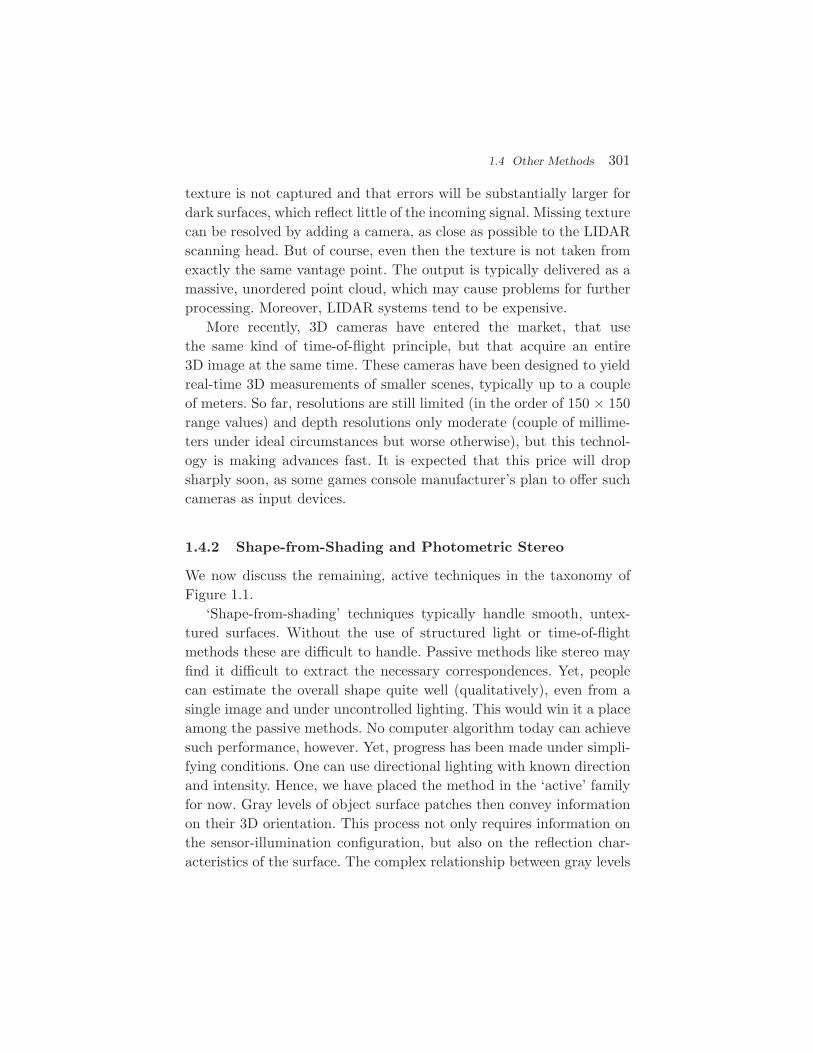
1.4.2 Shape-from-Shading and Photometric Stereo
We now discuss the remaining, active techniques in the taxonomy ofFigure 1.1.
‘Shape-from-shading’ techniques typically handle smooth, untex-tured surfaces. Without the use of structured light or time-of-flightmethods these are difficult to handle. Passive methods like stereo mayfind it difficult to extract the necessary correspondences. Yet, peoplecan estimate the overall shape quite well (qualitatively), even from asingle image and under uncontrolled lighting. This would win it a placeamong the passive methods. No computer algorithm today can achievesuch performance, however. Yet, progress has been made under simpli-fying conditions. One can use directional lighting with known directionand intensity. Hence, we have placed the method in the ‘active’ familyfor now. Gray levels of object surface patches then convey informationon their 3D orientation. This process not only requires information onthe sensor-illumination configuration, but also on the reflection char-acteristics of the surface. The complex relationship between gray levels

302 Introduction to 3D Acquisition
and surface orientation can theoretically be calculated in some cases —e.g., when the surface reflectance is known to be Lambertian — but isusually derived from experiments and then stored in ‘reflectance maps’for table-lookup. For a Lambertian surface with known albedo and fora known light source intensity, the angle between the surface normaland the incident light direction can be derived. This yields surface nor-mals that lie on a cone about the light direction. Hence, even in thissimple case, the normal of a patch cannot be derived uniquely fromits intensity. Therefore, information from different patches is combinedthrough extra assumptions on surface smoothness. Neighboring patchescan be expected to have similar normals. Moreover, for a smooth sur-face the normals at the visible rim of the object can be determinedfrom their tangents in the image if the camera settings are known.Indeed, the 3D normals are perpendicular to the plane formed by theprojection ray at these points and the local tangents to the boundaryin the image. This yields strong boundary conditions. Estimating thelighting conditions is sometimes made part of the problem. This maybe very useful, as in cases where the light source is the sun. The lightis also not always assumed to be coming from a single direction. Forinstance, some lighting models consist of both a directional componentand a homogeneous ambient component, where light is coming from alldirections in equal amounts. Surface interreflections are a complicationwhich these techniques so far cannot handle.
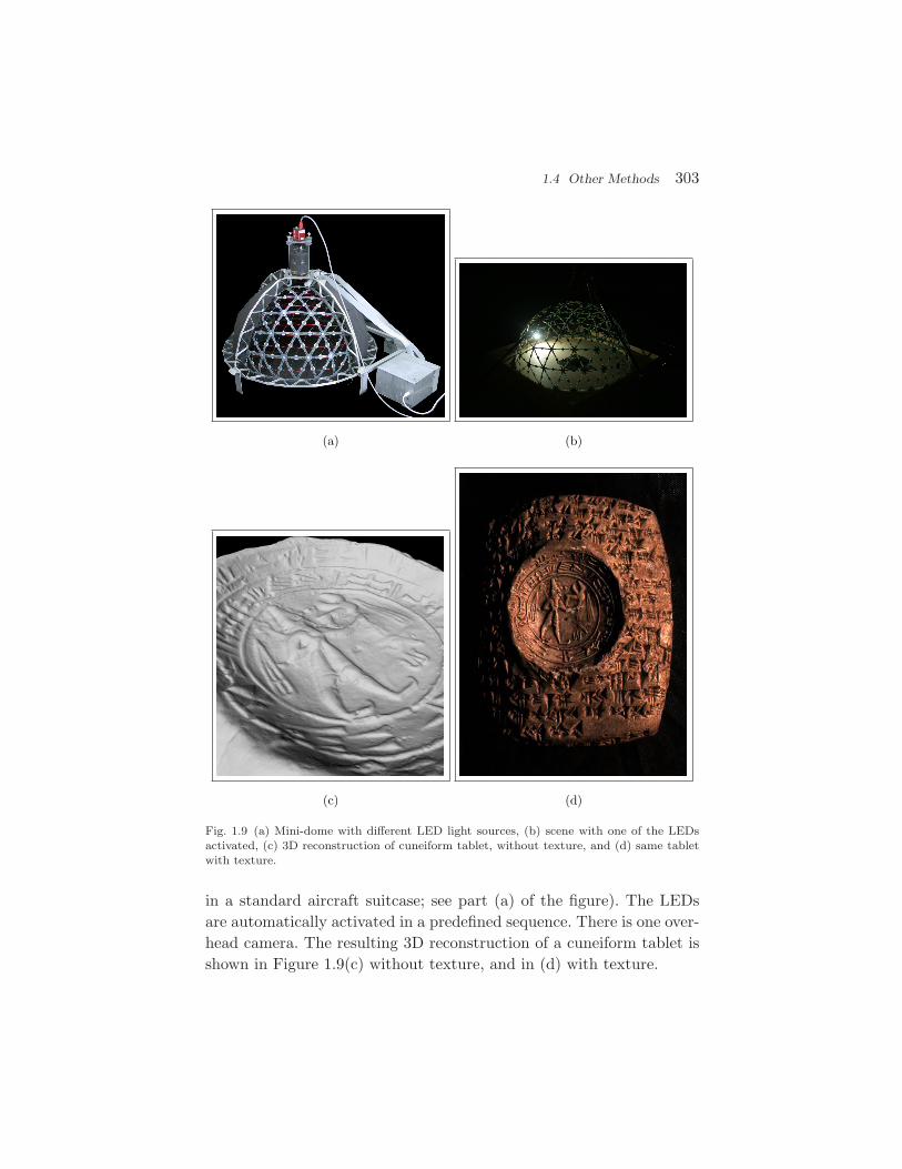
The need to combine normal information from different patches canbe reduced by using different light sources with different positions. Thelight sources are activated one after the other. The subsequent observedintensities for the surface patches yield only a single possible normalorientation (not withstanding noise in the intensity measurements).For a Lambertian surface, three different lighting directions suffice toeliminate uncertainties about the normal direction. The three conesintersect in a single line, which is the sought patch normal. Of course,it still is a good idea to further improve the results, e.g., via smoothnessassumptions. Such ‘photometric stereo’ approach is more stable thanshape-from-shading, but it requires a more controlled acquisition envi-ronment. An example is shown in Figure 1.9. It shows a dome with 260LEDs that is easy to assemble and disassemble (modular design, fitting
1.4 Other Methods 303
Fig. 1.9 (a) Mini-dome with different LED light sources, (b) scene with one of the LEDsactivated, (c) 3D reconstruction of cuneiform tablet, without texture, and (d) same tabletwith texture.
in a standard aircraft suitcase; see part (a) of the figure). The LEDsare automatically activated in a predefined sequence. There is one over-head camera. The resulting 3D reconstruction of a cuneiform tablet isshown in Figure 1.9(c) without texture, and in (d) with texture.

304 Introduction to 3D Acquisition
As with structured light techniques, one can try to reduce the num-ber of images that have to be taken, by giving the light sources differ-ent colors. The resulting mix of colors at a surface patch yields directinformation about the surface normal. In case 3 projections suffice, onecan exploit the R-G-B channels of a normal color camera. It is liketaking three intensity images in parallel, one per spectral band of thecamera.
Note that none of the above techniques yield absolute depths, butrather surface normal directions. These can be integrated into full3D models of shapes.
1.4.3 Shape-from-Texture and Shape-from-Contour
Passive single vantage methods include shape-from-texture and shape-from-contour. These methods do not yield true range data, but, as inthe case of shape-from-shading, only surface orientation.
Shape-from-texture assumes that a surface is covered by a homo-geneous texture (i.e., a surface pattern with some statistical or geo-metric regularity). Local inhomogeneities of the imaged texture (e.g.,anisotropy in the statistics of edge orientations for an isotropic tex-ture, or deviations from assumed periodicity) are regarded as the resultof projection. Surface orientations which allow the original texture tobe maximally isotropic or periodic are selected. Figure 1.10 shows an
Fig. 1.10 Left: The regular texture yields a clear perception of a curved surface. Right: theresult of a shape-from-texture algorithm.

1.4 Other Methods 305
example of a textured scene. The impression of an undulating surfaceis immediate. The right-hand side of the figure shows the results fora shape-from-texture algorithm that uses the regularity of the patternfor the estimation of the local surface orientation. Actually, what isassumed here is a square shape of the pattern’s period (i.e., a kindof discrete isotropy). This assumption suffices to calculate the localsurface orientation. The ellipses represent circles with such calculatedorientation of the local surface patch. The small stick at their centershows the computed normal to the surface.
Shape-from-contour makes similar assumptions about the trueshape of, usually planar, objects. Observing an ellipse, the assumptioncan be made that it actually is a circle, and the slant and tilt angles ofthe plane can be determined. For instance, in the shape-from-texturefigure we have visualized the local surface orientation via ellipses. This3D impression is compelling, because we tend to interpret the ellipticalshapes as projections of what in reality are circles. This is an exam-ple of shape-from-contour as applied by our brain. The circle–ellipserelation is just a particular example, and more general principles havebeen elaborated in the literature. An example is the maximization ofarea over perimeter squared, as a measure of shape compactness, overall possible deprojections, i.e., surface patch orientations. Returningto our example, an ellipse would be deprojected to a circle for thismeasure, consistent with human vision. Similarly, symmetries in theoriginal shape will get lost under projection. Choosing the slant andtilt angles that maximally restore symmetry is another example of acriterion for determining the normal to the shape. As a matter of fact,the circle–ellipse case also is an illustration for this measure. Regularfigures with at least a 3-fold rotational symmetry yield a single orien-tation that could make up for the deformation in the image, exceptfor the mirror reversal with respect to the image plane (assuming thatperspective distortions are too small to be picked up). This is but aspecial case of the more general result, that a unique orientation (up tomirror reflection) also results when two copies of a shape are observedin the same plane (with the exception where their orientation differs by0 or 180 in which case nothing can be said on the mere assumptionthat both shapes are identical). Both cases are more restrictive than

306 Introduction to 3D Acquisition
skewed mirror symmetry (without perspective effects), which yields aone-parameter family of solutions only.
1.4.4 Shape-from-Defocus
Cameras have a limited depth-of-field. Only points at a particulardistance will be imaged with a sharp projection in the image plane.Although often a nuisance, this effect can also be exploited because ityields information on the distance to the camera. The level of defocushas already been used to create depth maps. As points can be blurredbecause they are closer or farther from the camera than at the positionof focus, shape-from-defocus methods will usually combine more thana single image, taken from the same position but with different focallengths. This should disambiguate the depth.
1.4.5 Shape-from-Silhouettes
Shape-from-silhouettes is a passive, multi-vantage approach. Supposethat an object stands on a turntable. At regular rotational intervalsan image is taken. In each of the images, the silhouette of the objectis determined. Initially, one has a virtual lump of clay, larger than theobject and fully containing it. From each camera orientation, the silhou-ette forms a cone of projection rays, for which the intersection with thisvirtual lump is calculated. The result of all these intersections yields anapproximate shape, a so-called visual hull. Figure 1.11 illustrates theprocess.
One has to be careful that the silhouettes are extracted with goodprecision. A way to ease this process is by providing a simple back-ground, like a homogeneous blue or green cloth (‘blue keying’ or ‘greenkeying’). Once a part of the lump has been removed, it can never beretrieved in straightforward implementations of this idea. Therefore,more refined, probabilistic approaches have been proposed to fend offsuch dangers. Also, cavities that do not show up in any silhouette willnot be removed. For instance, the eye sockets in a face will not bedetected with such method and will remain filled up in the final model.This can be solved by also extracting stereo depth from neighboring

1.4 Other Methods 307
Fig. 1.11 The first three images show different backprojections from the silhouette of ateapot in three views. The intersection of these backprojections form the visual hull of theobject, shown in the bottom right image. The more views are taken, the closer the visualhull approaches the true shape, but cavities not visible in the silhouettes are not retrieved.
viewpoints and by combining the 3D information coming from bothmethods.
The hardware needed is minimal, and very low-cost shape-from-silhouette systems can be produced. If multiple cameras are placedaround the object, the images can be taken all at once and the capturetime can be reduced. This will increase the price, and also the silhouetteextraction may become more complicated. In the case video camerasare used, a dynamic scene like a moving person can be captured in 3Dover time (but note that synchronization issues are introduced). Anexample is shown in Figure 1.12, where 15 video cameras were set upin an outdoor environment.
Of course, in order to extract precise cones for the intersection, therelative camera positions and their internal settings have to be knownprecisely. This can be achieved with the same self-calibration methodsexpounded in the following sections. Hence, also shape-from-silhouettescan benefit from the presented ideas and this is all the more interesting

308 Introduction to 3D Acquisition
Fig. 1.12 (a) Fifteen cameras setup in an outdoor environment around a person,(b) a moredetailed view on the visual hull at a specific moment of the action,(c) detailed view on thevisual hull textured by backprojecting the image colors, and (d) another view of the visualhull with backprojected colors. Note how part of the sock area has been erroneously carvedaway.
1.5 Challenges 309
as this 3D extraction approach is among the most practically relevantones for dynamic scenes (‘motion capture’).
1.4.6 Hybrid Techniques
The aforementioned techniques often have complementary strengthsand weaknesses. Therefore, several systems try to exploit multiple tech-niques in conjunction. A typical example is the combination of shape-from-silhouettes with stereo as already hinted in the previous section.Both techniques are passive and use multiple cameras. The visual hullproduced from the silhouettes provides a depth range in which stereocan try to refine the surfaces in between the rims, in particular atthe cavities. Similarly, one can combine stereo with structured light.Rather than trying to generate a depth map from the images pure,one can project a random noise pattern, to make sure that there isenough texture. As still two cameras are used, the projected patterndoes not have to be analyzed in detail. Local pattern correlations maysuffice to solve the correspondence problem. One can project in thenear-infrared, to simultaneously take color images and retrieve the sur-face texture without interference from the projected pattern. So far,the problem with this has often been the weaker contrast obtainedin the near-infrared band. Many such integrated approaches can bethought of.
This said, there is no single 3D acquisition system to date that canhandle all types of objects or surfaces. Transparent or glossy surfaces(e.g., glass, metals), fine structures (e.g., hair or wires), and too weak,too busy, to too repetitive surface textures (e.g., identical tiles on awall) may cause problems, depending on the system that is being used.The next section discusses still existing challenges in a bit more detail.
1.5 Challenges
The production of 3D models has been a popular research topic alreadyfor a long time now, and important progress has indeed been made sincethe early days. Nonetheless, the research community is well aware ofthe fact that still much remains to be done. In this section we list someof these challenges.

310 Introduction to 3D Acquisition
As seen in the previous section, there is a wide variety of techniquesfor creating 3D models, but depending on the geometry and materialcharacteristics of the object or scene, one technique may be much bettersuited than another. For example, untextured objects are a nightmarefor traditional stereo, but too much texture may interfere with the pat-terns of structured-light techniques. Hence, one would seem to need abattery of systems to deal with the variability of objects — e.g., in amuseum — to be modeled. As a matter of fact, having to model theentire collections of diverse museums is a useful application area tothink about, as it poses many of the pending challenges, often severalat once. Another area is 3D city modeling, which has quickly grown inimportance over the last years. It is another extreme in terms of con-ditions under which data have to be captured, in that cities representan absolutely uncontrolled and large-scale environment. Also in thatapplication area, many problems remain to be resolved.
Here is a list of remaining challenges, which we don’t claim to beexhaustive:
• Many objects have an intricate shape, the scanning of whichrequires high precision combined with great agility of thescanner to capture narrow cavities and protrusions, deal withself-occlusions, fine carvings, etc.
• The types of objects and materials that potentially have to behandled — think of the museum example — are very diverse,like shiny metal coins, woven textiles, stone or wooden sculp-tures, ceramics, gems in jewellery and glass. No single tech-nology can deal with all these surface types and for some ofthese types of artifacts there are no satisfactory techniquesyet. Also, apart from the 3D shape the material characteris-tics may need to be captured as well.
• The objects to be scanned range from tiny ones like a needleto an entire construction or excavation site, landscape, orcity. Ideally, one would handle this range of scales with thesame techniques and similar protocols.
• For many applications, data collection may have to beundertaken on-site under potentially adverse conditions or

1.5 Challenges 311
implying transportation of equipment to remote or harshenvironments.
• Objects are sometimes too fragile or valuable to be touchedand need to be scanned ‘hands-off’. The scanner needs to bemoved around the object, without it being touched, usingportable systems.
• Masses of data often need to be captured, like in our museumcollection or city modeling examples. More efficient data cap-ture and model building are essential if this are to be prac-tical.
• Those undertaking the digitization may or may not be tech-nically trained. Not all applications are to be found in indus-try, and technically trained personnel may very well notbe around. This raises the need for intelligent devices thatensure high-quality data through (semi-)automation, self-diagnosis, and effective guidance of the operator.
• In many application areas the money that can be spent isvery limited and solutions therefore need to be relativelycheap.
• Also, precision is a moving target in many applications andas higher precisions are achieved, new applications presentthemselves that push for going even beyond. Analyzing the3D surface of paintings to study brush strokes is a case inpoint.
These considerations about the particular conditions under whichmodels may need to be produced, lead to a number of desirable, tech-nological developments for 3D data acquisition:
• Combined extraction of shape and surface reflectance.Increasingly, 3D scanning technology is aimed at also extract-ing high-quality surface reflectance information. Yet, therestill is an appreciable way to go before high-precision geom-etry can be combined with detailed surface characteristicslike full-fledged BRDF (Bidirectional Reflectance Distribu-tion Function) or BTF (Bidirectional Texture Function)information.

312 Introduction to 3D Acquisition
• In-hand scanning. The first truly portable scanning systemsare already around. But the choice is still restricted, espe-cially when also surface reflectance information is requiredand when the method ought to work with all types of mate-rials, including metals, glass, etc. Also, transportable hereis supposed to mean more than ‘can be dragged betweenplaces’, i.e., rather the possibility to easily move the systemaround the object, ideally also by hand. But there also is theinteresting alternative to take the objects to be scanned inone’s hands, and to manipulate them such that all parts getexposed to the fixed scanner. This is not always a desirableoption (e.g., in the case of very valuable or heavy pieces), buthas the definite advantage of exploiting the human agilityin presenting the object and in selecting optimal, additionalviews.
• On-line scanning. The physical action of scanning and theactual processing of the data often still are two separatesteps. This may create problems in that the completenessand quality of the result can only be inspected after thescanning session is over and the data are analyzed and com-bined at the lab or the office. It may then be too late ortoo cumbersome to take corrective actions, like taking a fewadditional scans. It would be very desirable if the systemwould extract the 3D data on the fly, and would give imme-diate visual feedback. This should ideally include steps likethe integration and remeshing of partial scans. This wouldalso be a great help in planning where to take the next scanduring scanning. A refinement can then still be performedoff-line.
• Opportunistic scanning. Not a single 3D acquisition tech-nique is currently able to produce 3D models of even a largemajority of exhibits in a typical museum. Yet, they often havecomplementary strengths and weaknesses. Untextured sur-faces are a nightmare for passive techniques, but may be idealfor structured light approaches. Ideally, scanners would auto-matically adapt their strategy to the object at hand, based

1.5 Challenges 313
on characteristics like spectral reflectance, texture spatialfrequency, surface smoothness, glossiness, etc. One strategywould be to build a single scanner that can switch strategyon-the-fly. Such a scanner may consist of multiple camerasand projection devices, and by today’s technology could stillbe small and light-weight.
• Multi-modal scanning. Scanning may not only combinegeometry and visual characteristics. Additional features likenon-visible wavelengths (UV,(N)IR) could have to be cap-tured, as well as haptic impressions. The latter would thenalso allow for a full replay to the public, where audiences canhold even the most precious objects virtually in their hands,and explore them with all their senses.
• Semantic 3D. Gradually computer vision is getting at apoint where scene understanding becomes feasible. Out of 2Dimages, objects and scene types can be recognized. This willin turn have a drastic effect on the way in which ‘low’-levelprocesses can be carried out. If high-level, semantic interpre-tations can be fed back into ‘low’-level processes like motionand depth extraction, these can benefit greatly. This strat-egy ties in with the opportunistic scanning idea. Recognizingwhat it is that is to be reconstructed in 3D (e.g., a car andits parts) can help a system to decide how best to go about,resulting in increased speed, robustness, and accuracy. It canprovide strong priors about the expected shape and surfacecharacteristics.
• Off-the-shelf components. In order to keep 3D modelingcheap, one would ideally construct the 3D reconstruction sys-tems on the basis of off-the-shelf, consumer products. At leastas much as possible. This does not only reduce the price, butalso lets the systems surf on a wave of fast-evolving, mass-market products. For instance, the resolution of still, digitalcameras is steadily on the increase, so a system based onsuch camera(s) can be upgraded to higher quality withoutmuch effort or investment. Moreover, as most users will beacquainted with such components, the learning curve to use

314 Introduction to 3D Acquisition
the system is probably not as steep as with a totally novel,dedicated technology.
Obviously, once 3D data have been acquired, further process-ing steps are typically needed. These entail challenges of their own.Improvements in automatic remeshing and decimation are definitelystill possible. Also solving large 3D puzzles automatically, preferablyexploiting shape in combination with texture information, would besomething in high demand from several application areas. Level-of-detail (LoD) processing is another example. All these can also beexpected to greatly benefit from a semantic understanding of the data.Surface curvature alone is a weak indicator of the importance of a shapefeature in LoD processing. Knowing one is at the edge of a salient, func-tionally important structure may be a much better reason to keep it inat many scales.
1.6 Conclusions
Given the above considerations, the 3D reconstruction of shapes frommultiple, uncalibrated images is one of the most promising 3D acquisi-tion techniques. In terms of our taxonomy of techniques, self-calibratingstructure-from-motion ia a passive, multi-vantage point strategy. Itoffers high degrees of flexibility in that one can freely move a cameraaround an object or scene. The camera can be hand-held. Most peoplehave a camera and know how to use it. Objects or scenes can be smallor large, assuming that the optics and the amount of camera motionare appropriate. These methods also give direct access to both shapeand surface reflectance information, where both can be aligned withoutspecial alignment techniques. Efficient implementations of several sub-parts of such SfM pipelines have been proposed lately, so that the on-line application of such methods is gradually becoming a reality. Also,the required hardware is minimal, and in many cases consumer typecameras will suffice. This keeps prices for data capture relatively low.
2Principles of Passive 3D Reconstruction
2.1 Introduction
In this section the basic principles underlying self-calibrating, passive3D reconstruction, are explained. More specifically, the central goal is toarrive at a 3D reconstruction from the uncalibrated image data alone.But, to understand how three-dimensional (3D) objects can be recon-structed from two-dimensional (2D) images, one first needs to knowhow the reverse process works: i.e., how images of a 3D object arise.Section 2.2 therefore discusses the image formation process in a cameraand introduces the camera model which will be used throughout thetext. As will become clear this model incorporates internal and exter-nal parameters related to the technical specifications of the camera(s)and their location with respect to the objects in the scene. Subsequentsections then set out to extract 3D models of the scene without priorknowledge of these parameters, i.e., without the need to calibrate thecameras internally or externally first. This reconstruction problem isformulated mathematically in Section 2.3 and a solution strategy isinitiated. The different parts in this solution of the 3D reconstructionproblem are elaborated in the following sections. Along the way, fun-damental notions such as the correspondence problem, the epipolar
315

316 Principles of Passive 3D Reconstruction
relation, and the fundamental matrix of an image pair are introduced(Section 2.4), and the possible stratification of the reconstruction pro-cess into Euclidean, metric, affine, and projective reconstructions isexplained (Section 2.5). Furthermore, self-calibration equations arederived and their solution is discussed in Section 2.6. Apart fromthe generic case, special camera motions are considered as well (Sec-tion 2.7). In particular, camera translation rotations are discussed.These often occur in practice, but their systems of self-calibration equa-tions or reconstruction equations become singular. Attention is paidalso to the case of internally calibrated cameras and the importantnotion and use of the essential matrix is explored for that case.
As a note on widely used terminology in this domain, the wordcamera is often to be interpreted as a certain viewpoint and viewingdirection — a field of view or image — and if mention is made of afirst, second, . . . camera then this can just as well refer to the samecamera being moved around to a first, second, . . . position.
2.2 Image Formation and Camera Model
2.2.1 The Pinhole Camera
The simplest model of the image formation process in a camera is thatof a pinhole camera or camera obscura. The camera obscura is notmore than a black box one side of which is punctured to yield a smallhole. The rays of light from the outside world that pass through thehole and fall on the opposite side of the box there form a 2D image ofthe 3D environment outside the box (called the scene), as is depictedin Figure 2.1. Some art historians believe that the painter Vermeeractually used a room-sized version of a camera obscura. Observe thatthis pinhole image actually is the photo-negative image of the scene.The photo-positive image one observes when watching a photographor a computer screen corresponds to the projection of the scene onto ahypothetical plane that is situated in front of the camera obscura at thesame distance from the hole as the opposite wall on which the image isactually formed. In the sequel, the term image plane will always refer tothis hypothetical plane in front of the camera. This hypothetical planeis preferred to avoid sign reversals in the computations. The distance

2.2 Image Formation and Camera Model 317
Fig. 2.1 In a pinhole camera or camera obscura an image of the scene is formed by the raysof light that are reflected by the objects in the scene and fall through the center of projectiononto the opposite wall of the box, forming a photo-negative image of the scene. The photo-positive image of the scene corresponds to the projection of the scene onto a hypotheticalimage plane situated in front of the camera. It is this hypothetical plane which is typicallyused in computer vision, in order to avoid sign reversals.
between the center of projection (the hole) and the image plane is calledthe focal length of the camera.
The amount of light that falls into the box through the small holeis very limited. One can increase this amount of light by making thehole bigger, but then rays coming from different 3D points can fallonto the same point on the image, thereby causing blur. One way ofgetting around this problem is by making use of lenses, which focus thelight. Apart from the introduction of geometric and chromatic aberra-tions, even the most perfect lens will come with a limited depth-of-field.This means that only scene points within a limited depth range areimaged sharply. Within that depth range the camera with lens basi-cally behaves like the pinhole model. The ‘hole’ in the box will in thesequel be referred to as the center of projection or the camera center,and the type of projection realized by this idealized model is referredto as perspective projection.
It has to be noted that whereas in principle a single convex lensemight be used, real camera lenses are composed of multiple lenses, inorder to reduce deviations from the ideal model (i.e., to reduce theaforementioned aberrations). A detailed discussion on this importantoptical component is out of the scope of this tutorial, however.

318 Principles of Passive 3D Reconstruction
2.2.2 Projection Equations for a Camera-CenteredReference Frame
To translate the image formation process into mathematical formulaswe first introduce a reference frame for the 3D environment (also calledthe world) containing the scene. The easiest is to fix it to the camera.Figure 2.2 shows such a camera-centered reference frame. It is a right-handed and orthonormal reference frame whose origin is at the center ofprojection. Its Z-axis is the principal axis of the camera, — i.e., the linethrough the center of projection and orthogonal to the image plane —and the XY -plane is the plane through the center of projection andparallel to the image plane. The image plane is the plane with equationZ = f , where f denotes the focal length of the camera. The principalaxis intersects the image plane in the principal point p.
The camera-centered reference frame induces an orthonormal uv
reference frame in the image plane, as depicted in Figure 2.2. Theimage of a scene point M is the point m where the line through M andthe origin of the camera-centered reference frame intersects the imageplane. If M has coordinates (X,Y,Z) ∈ R
3 with respect to the camera-centered reference frame, then an arbitrary point on the line through
X
Y
Z
uvC
pM
mCenter ofprojection
Image planePrincipal axis
Principal point
Fig. 2.2 The camera-centered reference frame is fixed to the camera and aligned with itsintrinsic directions, of which the principal axis is one. The coordinates of the projection mof a scene point M onto the image plane in a pinhole camera model with a camera-centeredreference frame, as expressed by equation (2.1), are given with respect to the principalpoint p in the image.

2.2 Image Formation and Camera Model 319
the origin and the scene point M has coordinates ρ(X,Y,Z) for somereal number ρ. The point of intersection of this line with the imageplane must satisfy the relation ρZ = f , or equivalently, ρ = f
Z . Hence,the image m of the scene point M has coordinates (u,v,f), where
u = fX
Zand v = f
Y
Z. (2.1)
Projections onto the image plane cannot be detected with infiniteprecision. An image rather consists of physical cells capturing photons,so-called picture elements, or pixels for short. Apart from some exoticdesigns (e.g., hexagonal or log-polar cameras), these pixels are arrangedin a rectangular grid, i.e., according to rows and columns, as depictedin Figure 2.3 (left). Pixel positions are typically indicated with a rowand column number measured with respect to the top left corner ofthe image. These numbers are called the pixel coordinates of an imagepoint. We will denote them by (x,y), where the x-coordinate is mea-sured horizontally and increasing to the right, and the y-coordinate ismeasured vertically and increasing downwards. This choice has severaladvantages:
• The way in which x- and y-coordinates are assigned to imagepoints corresponds directly to the way in which an image isread out by several digital cameras with a CCD: starting atthe top left and reading line by line.
x
y
p u
vv~
u~0
pu
pv
Fig. 2.3 Left: In a digital image, the position of a point in the image is indicated by itspixel coordinates. This corresponds to the way in which a digital image is read from a CCD.Right: The coordinates (u,v) of the projection of a scene point in the image are definedwith respect to the principal point p. Pixel coordinates, on the other hand, are measureswith respect to the upper left corner of the image.

320 Principles of Passive 3D Reconstruction
• The camera-centered reference frame for the world beingright-handed then implies that its Z-axis is pointing awayfrom the image into the scene (as opposed to into the cam-era). Hence, the Z-coordinate of a scene point correspondsto the “depth” of that point with respect to the camera,which conceptually is nice because it is the big unknown tobe solved for in 3D reconstruction problems.
As a consequence, we are not so much interested in the metric coordi-nates (u,v) indicating the projection m of a scene point M in the imageand given by formula (2.1), as in the corresponding row and columnnumbers (x,y) of the underlying pixel. At the end of the day, it willbe these pixel coordinates to which we have access when analyzing theimage. Therefore we have to make the transition from (u,v)-coordinatesto pixel coordinates (x,y) explicit first.
In a camera-centered reference frame the X-axis is typically chosenparallel to the rows and the Y -axis parallel to the columns of the rect-angular grid of pixels. In this way, the u- and v-axes induced in theimage plane have the same direction and sense as those in which thepixel coordinates x and y of image points are measured. But, whereaspixel coordinates are measured with respect to the top left corner ofthe image, (u,v)-coordinates are measured with respect to the principalpoint p. The first step in the transition from (u,v)- to (x,y)-coordinatesfor an image point m thus is to apply offsets to each coordinate. To thisend, denoted by pu and pv the metric distances, measured in the hori-zontal and vertical directions, respectively, of the principal point p fromthe upper left corner of the image (see Figure 2.3 (right) ). With thetop left corner of the image as origin, the principal point now has coor-dinates (pu,pv) and the perspective projection m of the scene point M,as described by formula (2.1), will have coordinates
u = fX
Z+ pu and v = f
Y
Z+ pv.
These (u, v)-coordinates of the image point m are still expressed in themetric units of the camera-centered reference frame. To convert them topixel coordinates, one has to divide u and v by the width and the heightof a pixel, respectively. Let mu and mv be the inverse of resprespectively

2.2 Image Formation and Camera Model 321
the pixel width and height, then mu and mv indicate how many pixelsfit into one horizontal resprespectively vertical metric unit. The pixelcoordinates (x,y) of the projection m of the scene point M in the imageare thus given by
x = mu
(f
X
Z+ pu
)and y = mv
(f
Y
Z+ pv
);
or equivalently,
x = αxX
Z+ px and y = αy
Y
Z+ py, (2.2)
where αx = mu f and αy = mv f is the focal length expressed in numberof pixels for the x- and y-direction of the image and (px,py) are thepixel coordinates of the principal point. The ratio αy
αx= mv
mu, giving the
ratio of the pixel width with respect to the pixel height, is called theaspect ratio of the pixels.
2.2.3 A Matrix Expression for Camera-Centered Projection
More elegant expressions for the projection Equation (2.2) are obtainedif one uses extended pixel coordinates for the image points. In particular,if a point m with pixel coordinates (x,y) in the image is represented bythe column vector m = (x,y,1)T , then formula (2.2) can be rewrittenas:
Z m = Z
x
y
1
=
αx 0 px
0 αy py
0 0 1
X
Y
Z
. (2.3)
Observe that, if one interpretes the extended pixel coordinates (x,y,1)T
of the image point m as a vector indicating a direction in the world,then, since Z describes the “depth” in front of the camera at which thecorresponding scene point M is located, the 3 × 3-matrix
αx 0 px
0 αy py
0 0 1
represents the transformation that converts world measurements(expressed in meters, centimeters, millimeters, . . . ) into the pixel met-ric of the digital image. This matrix is called the calibration matrix

322 Principles of Passive 3D Reconstruction
of the camera, and it is generally represented as the upper triangularmatrix
K =
αx s px
0 αy py
0 0 1
, (2.4)
where αx and αy are the focal lengths expressed in number of pixelsfor the x- and y-directions in the image and with (px,py) the pixelcoordinates of the principal point. The additional scalar s in the cal-ibration matrix K is called the skew factor and models the situationin which the pixels are parallelograms (i.e., not rectangular). It alsoyields an approximation to the situation in which the physical imagingplane is not perfectly perpendicular to the optical axis of the lens orobjective (as was assumed above). In fact, s is inversely proportional tothe tangent of the angle between the X- and the Y -axis of the camera-centered reference frame. Consequently, s = 0 for digital cameras withrectangular pixels.
Together, the entries αx, αy, s, px, and py of the calibrationmatrix K describe the internal behavior of the camera and are there-fore called the internal parameters of the camera. Furthermore, theprojection Equation (2.3) of a pinhole camera with respect to a camera-centered reference frame for the scene are compactly written as:
ρm = KM, (2.5)
where M = (X,Y,Z)T are the coordinates of a scene point M with respectto the camera-centered reference frame for the scene, m = (x,y,1)T arethe extended pixel coordinates of its projection m in the image, K isthe calibration matrix of the camera. Furthermore, ρ is a positive realnumber and it actually represents the “depth” of the scene point M
in front of the camera, because, due to the structure of the calibra-tion matrix K, the third row in the matrix Equation (2.5) reduces toρ = Z. Therefore ρ is called the projective depth of the scene point M
corresponding to the image point m.
2.2.4 The General Linear Camera Model
When more than one camera is used, or when the objects in the sceneare to be represented with respect to another, non-camera-centered

2.2 Image Formation and Camera Model 323
X
Y
Z
0
C
r1
r2
r3
u
v
M = (X,Y,Z)
(u,v)
Fig. 2.4 The position and orientation of the camera in the scene are given by a positionvector C and a 3 × 3-rotation matrix R. The projection m of a scene point M is then givenby formula (2.6).
reference frame (called the world frame), then the position and orien-tation of the camera in the scene are described by a point C, indicat-ing the center of projection, and a 3 × 3-rotation matrix R indicatingthe orientation of the camera-centered reference frame with respect tothe world frame. More precisely, the column vectors ri of the rotationmatrix R are the unit direction vectors of the coordinate axes of thecamera-centered reference frame, as depicted in Figure 2.4. As C andR represent the setup of the camera in the world space, they are calledthe external parameters of the camera.
The coordinates of a scene point M with respect to the camera-centered reference frame are found by projecting the relative posi-tion vector M − C orthogonally onto each of the coordinate axes of thecamera-centered reference frame. The column vectors ri of the rotationmatrix R being the unit direction vectors of the coordinate axes of thecamera-centered reference frame, the coordinates of M with respect tothe camera-centered reference frame are given by the dot products ofthe relative position vector M − C with the unit vectors ri; or equiva-lently, by premultiplying the column vector M − C with the transposeof the orientation matrix R, viz. RT (M − C). Hence, following Equa-tion (2.5), the projection m of the scene point M in the image is givenby the (general) projection equations:
ρm = KRT (M − C), (2.6)

324 Principles of Passive 3D Reconstruction
where M = (X,Y,Z)T are the coordinates of a scene point M with respectto an (arbitrary) world frame, m = (x,y,1)T are the extended pixel coor-dinates of its projection m in the image, K is the calibration matrix ofthe camera, C is the position and R is the rotation matrix expressingthe orientation of the camera with respect to the world frame, and ρ isa positive real number representing the projective depth of the scenepoint M with respect to the camera.
Many authors prefer to use extended coordinates for scene points aswell. So, if
(M1
)= (X,Y,Z,1)T are the extended coordinates of the scene
point M = (X,Y,Z)T , then the projection Equation (2.6) becomes
ρm =(KRT | −KRTC
)(M1
). (2.7)
The 3 × 4-matrix P = (KRT | −KRTC) is called the projection matrixof the camera.
Notice that, if only the 3 × 4-projection matrix P is known, it ispossible to retrieve the internal and external camera parameters from it.Indeed, as is seen from formula (2.7), the upper left 3 × 3-submatrix ofP is formed by multiplying K and RT . Its inverse is RK−1, since R is arotation matrix and thus RT = R−1. Furthermore, K is a non-singularupper triangular matrix and so is K−1. In particular, RK−1 is the prod-uct of an orthogonal matrix and an upper triangular one. Recall fromlinear algebra that every 3 × 3-matrix of maximal rank can uniquely bedecomposed as a product of an orthogonal and a non-singular, uppertriangular matrix with positive diagonal entries by means of the QR-decomposition [3] (with Q the orthogonal and R the upper-diagonalmatrix). Hence, given the 3 × 4-projection matrix P of a pinhole cam-era, the calibration matrix K and the orientation matrix R of thecamera can easily be recovered from the inverse of the upper left 3 × 3-submatrix of P by means of QR-decomposition. If K and R are known,then the center of projection C is found by premultiplying the fourthcolumn of P with the matrix −RK−1.
The camera model of Equation (2.7) is usually referred to as thegeneral linear camera model. Taking a close look at this formula showshow general the camera projection matrix P = (KRT | −KRTC) is asa matrix, in fact. Apart from the fact that the 3 × 3-submatrix on

2.2 Image Formation and Camera Model 325
the left has to be full rank, one cannot demand more than that ithas to be QR-decomposable, which holds for any such matrix. Theattentive reader may now object that, according to formula (2.4), thecalibration matrix K must have entry 1 at the third position in thelast row, whereas there is no such constraint for the upper triangularmatrix in a QR-decomposition. This would seem a further restrictionon the left 3 × 3-submatrix of P, but it can easily be lifted by observingthat the camera projection matrix P is actually only determined up toa scalar factor. Indeed, due to the non-zero scalar factor ρ in the left-hand side of formula (2.7), one can always ensure this property to hold.Put differently, any 3 × 4-matrix whose upper left 3 × 3-submatrix isnon-singular can be interpreted as the projection matrix of a (linear)pinhole camera.
2.2.5 Non-linear Distortions
The perspective projection model described in the previous sections islinear in the sense that the scene point, the corresponding image pointand the center of projection are collinear, and that straight lines in thescene do generate straight lines in the image. Perspective projectiontherefore only models the linear effects in the image formation pro-cess. Images taken by real cameras, on the other hand, also experiencenon-linear deformations or distortions which make the simple linearpinhole model inaccurate. The most important and best known non-linear distortion is radial distortion. Figure 2.5(left) shows an exampleof a radially distorted image. Radial distortion is caused by a system-atic variation of the optical magnification when radially moving awayfrom a certain point, called the center of distortion. The larger the dis-tance between an image point and the center of distortion, the largerthe effect of the distortion. Thus, the effect of the distortion is mostlyvisible near the edges of the image. This can clearly be seen in Fig-ure 2.5 (left). Straight lines near the edges of the image are no longerstraight but are bent. For practical use, the center of radial distortioncan often be assumed to coincide with the principal point, which usu-ally also coincides with the center of the image. But it should be notedthat these are only approximations and dependent on the accuracyrequirements, a more precise determination may be necessary [7].

326 Principles of Passive 3D Reconstruction
Fig. 2.5 Left: An image exhibiting radial distortion. The vertical wall at the left of thebuilding appears bent in the image and the gutter on frontal wall on the right appearscurved too. Right: The same image after removal of the radial distortion. Straight lines inthe scene now appear as straight lines in the image as well.
Radial distortion is a non-linear effect and is typically modeled usinga Taylor expansion. Typically, only the even order terms play a rolein this expansion, i.e., the effect is symmetric around the center. Theeffect takes place in the lens, hence mathematically the radial distortionshould be between the external and internal parameters of the pinholemodel. The model we will propose here follows this strategy. Let usdefine
ρ mu =
mux
muy
1
= RT (M − C) ,
where M = (X,Y,Z)T are the coordinates of a scene point with respectto the world frame. The distance r of the point mu from the optical axisis then
r2 = m2ux + m2
uy.
We now define md as
md =
mdx
mdy
1
=
(1 + κ1r2 + κ2r
4 + κ3r6 + . . .)mux
(1 + κ1r2 + κ2r
4 + κ3r6 + . . .)muy
1
. (2.8)
2.2 Image Formation and Camera Model 327
The lower order terms of this expansion are the most important onesand typically one does not compute more than three parameters (κ1,κ2, κ3). Finally the projection m of the 3D point M is:
m = Kmd. (2.9)
When the distortion parameters are known, the image can be undis-torted in order to make all lines straight again and thus make the lin-ear pinhole model valid. The undistorted version of Figure 2.5 (left) isshown in the same Figure 2.5 (right).
The model described above puts the radial distortion parametersbetween the external and linear internal parameters of the camera. Inthe literature one often finds that the distortion is put on the left of theinternal parameters, i.e., a 3D point is first projected into the imagevia the linear model and then shifted. Conceptually the latter model isless suited than the one used here because putting the distortion at theend makes it dependent on the internal parameters, especially on thefocal length. This means one has to re-estimate the radial distortionparameters every time the focal length changes. This is not necessaryin the model as suggested here. This, however, does not mean that thismodel is perfect. In reality the center of radial distortion (now assumedto be the principal point) sometimes changes when the focal length isaltered. This effect cannot be modeled with this approach.
In the remainder of the text we will assume that radial distortionhas been removed from all images if present, unless stated otherwise.
2.2.6 Explicit Camera Calibration
As explained before a perspective camera can be described by its inter-nal and external parameters. The process of determining these param-eters is known as camera calibration. Accordingly, we make a distinc-tion between internal or internal calibration and external or externalcalibration, also known as pose estimation. For the determination ofall parameters one often uses the term complete calibration. Tradi-tional 3D passive reconstruction techniques had a separate, explicitcamera calibration step. As highlighted before, the difference with self-calibration techniques as explained in this tutorial is that in the latter

328 Principles of Passive 3D Reconstruction
Fig. 2.6 Calibration objects: 3D (left) and 2D (right).
the same images used for 3D scene reconstruction are also used forcamera calibration.
Traditional internal calibration procedures [1, 17, 18] extract thecamera parameters from a set of known 3D–2D correspondences, i.e., aset of 3D coordinates with corresponding 2D coordinates in the imagefor their projections. In order to easily obtain such 3D–2D correspon-dences, they employ special calibration objects, like the ones displayedin Figure 2.6. These objects contain easily recognizable markers. Inter-nal calibration sometimes starts by fitting a linearized calibration modelto the 3D–2D correspondences, which is then improved with a subse-quent non-linear optimization step.
Some applications do not suffer from unknown scales or effects ofprojection, but their results would deteriorate under the influence ofnon-linear effects like radial distortion. It is possible to only undo suchdistortion without having to go through the entire process of internalcalibration. One way is by detecting structures that are known to bestraight, but appear curved under the influence of the radial distortion.Then, for each line (e.g., the curved roof top in the example of Figure 2.5(left)), points are sampled along it and a straight line is fitted throughthese data. If we want the distortion to vanish, the error consistingof the sum of the distances of each point to their line should be zero.Hence a non-linear minimization algorithm like Levenberg–Marquardtis applied to these data. The algorithm is initialized with the distortionparameters set to zero. At every iteration, new values are computed forthese parameters, the points are warped accordingly and new lines are

2.3 The 3D Reconstruction Problem 329
fitted. The algorithm stops when it converges to a solution where allselected lines are straight (i.e., the resulting error is close to zero). Theresulting unwarped image can be seen on the right in Figure 2.5.
2.3 The 3D Reconstruction Problem
The aim of passive 3D reconstruction is to recover the geometric struc-ture of a (static) scene from one or more of its images: Given a point min an image, determine the point M in the scene of which m is the projec-tion. Or, in mathematical parlance, given the pixel coordinates (x,y) ofa point m in a digital image, determine the world coordinates (X,Y,Z)of the scene point M of which m is the projection in the image. As can beobserved from the schematic representation of Figure 2.7, a point m inthe image can be the projection of any point M in the world space thatlies on the line through the center of projection and the image point m.Such line is called the projecting ray or the line of sight of the imagepoint m in the given camera. Thus, 3D reconstruction from one imageis an underdetermined problem.
On the other hand, if two images of the scene are available, the posi-tion of a scene point M can be recovered from its projections m1 and m2 inthe images by triangulation: M is the point of intersection of the project-ing rays of m1 and m2, as depicted in Figure 2.8. This stereo setup andthe corresponding principle of triangulation have already been intro-
image
C
m
M
Fig. 2.7 3D reconstruction from one image is an underdetermined problem: a point m in theimage can be the projection of any world point M along the projecting ray of m.

330 Principles of Passive 3D Reconstruction
image 1
C1
m1
image 2
m2
C2
M
Fig. 2.8 Given two images of a static scene, the location of the scene point M can be recoveredfrom its projections m1 and m2 in the respective images by means of triangulation.
duced in Section 1. As already noted there, the 3D reconstruction prob-lem has not yet been solved, unless the internal and external parametersof the cameras are known. Indeed, if we assume that the images arecorrected for radial distortion and other non-linear effects and that thegeneral linear pinhole camera model is applicable, then, according toEquation (2.6) in Section 2.2.4, the projection equations of the firstcamera are modeled as:
ρ1m1 = K1RT1 (M − C1), (2.10)
where M = (X,Y,Z)T are the coordinates of the scene point M withrespect to the world frame, m1 = (x1,y1,1)T are the extended pixelcoordinates of its projection m1 in the first image, K1 is the calibrationmatrix of the first camera, C1 is the position and R1 is the orientationof the first camera with respect to the world frame, and ρ1 is a positivereal number representing the projective depth of M with respect to thefirst camera. To find the projecting ray of an image point m1 in thefirst camera and therefore all points projecting onto m1 there, recallfrom Section 2.2.3 that the calibration matrix K1 converts world mea-surements (expressed in meters, centimeters, millimeters, etc) into thepixel metric of the digital image. Since m1 = (x1,y1,1) are the extendedpixel coordinates of the point m1 in the first image, the direction ofthe projecting ray of m1 in the camera-centered reference frame of thefirst camera is given by the three-vector K−1
1 m1. With respect to the

2.3 The 3D Reconstruction Problem 331
world frame, the direction vector of the projecting ray is R1K−11 m1, by
definition of R1. As the position of the first camera in the world frameis given by the point C1, the parameter equations of the projecting rayof m1 in the world frame are:
M = C1 + ρ1R1K−11 m1 for some ρ1 ∈ R. (2.11)
So, every scene point M satisfying Equation (2.11) for some real numberρ1 projects onto the point m1 in the first image. Notice that Equa-tion (2.11) can be found directly by solving the projection Equa-tion (2.10) for M. Clearly, the parameter Equation (2.11) of the project-ing ray of a point m1 in the first image are only fully known, providedthe calibration matrix K1 and the position C1 and orientation R1 ofthe camera with respect to the world frame are known (i.e., when thefirst camera is fully calibrated).
Similarly, the projection equations for the second camera are:
ρ2m2 = K2RT2 (M − C2), (2.12)
where m2 = (x2,y2,1)T are the extended pixel coordinates of M’s projec-tion m2 in the second image, K2 is the calibration matrix of the secondcamera, C2 is the position and R2 the orientation of the second camerawith respect to the world frame, and ρ2 is a positive real number rep-resenting the projective depth of M with respect to the second camera.Solving Equation (2.12) for M yields:
M = C2 + ρ2R2K−12 m2; (2.13)
and, if in this equation ρ2 is seen as a parameter, then formula (2.13) isjust the parameter equation for the projecting ray of the image point m2
in the second camera. Again, these parameter equations are fully knownonly if K2, C2, and R2 are known (i.e., when the second camera is fullycalibrated). The system of six Equations (2.10) and (2.12) can be solvedfor the five unknowns X, Y , Z, ρ1, and ρ2. Observe that this requiresthe system to be rank-deficient, which is guaranteed if the points m1
and m2 are in correspondence (i.e., their projecting rays intersect) andtherefore special relations (in particular, the so-called epipolar relations,which will be derived in the next section) hold.

332 Principles of Passive 3D Reconstruction
When the cameras are not internally and externally calibrated, thenit is not immediately clear how to perform triangulation from the imagedata alone. On the other hand, one intuitively feels that every imageof a static scene constrains in one way or another the shape and therelative positioning of the objects in the world, even if no informationabout the camera parameters is known. The key to the solution of the3D reconstruction problem is found in understanding how the locationsm1 and m2 of the projections of a scene point M in different views arerelated to each other. This relationship is explored in the next section.
2.4 The Epipolar Relation Between 2 Images of a StaticScene
2.4.1 The Fundamental Matrix
A point m1 in a first image of the scene is the projection of a scenepoint M that can be at any position along the projecting ray of m1 in thatfirst camera. Therefore, the corresponding point m2 (i.e., the projectionof M) in a second image of the scene must lie on the projection 2
of this projecting ray in the second image, as depicted in Figure 2.9.To derive the equation of this projection 2, suppose for a momentthat the internal and external parameters of both cameras are known.Then, the projecting ray of the point m1 in the first camera is given
l2
image 2
C2
m2
M
m1
image 1
C1
Fig. 2.9 The point m2 in the second image corresponding to a point m1 in the first imagelies on the epipolar line 2 which is the projection in the second image of the projecting rayof m1 in the first camera.
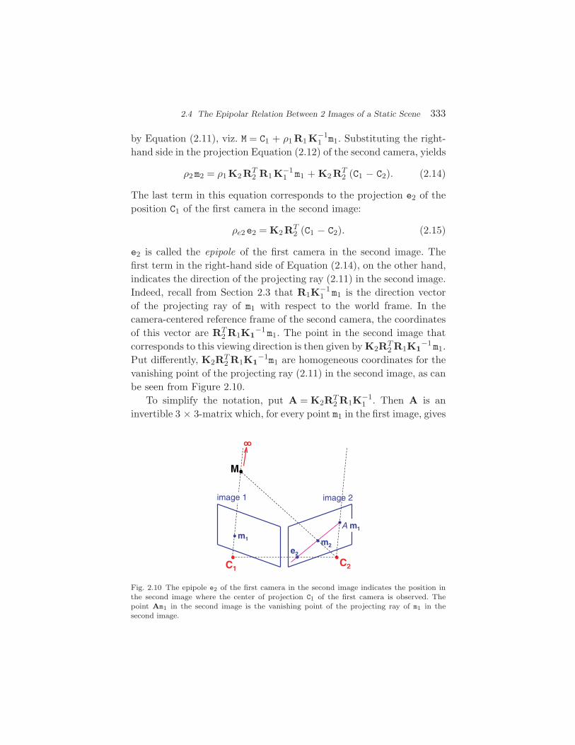
2.4 The Epipolar Relation Between 2 Images of a Static Scene 333
by Equation (2.11), viz. M = C1 + ρ1R1K−11 m1. Substituting the right-
hand side in the projection Equation (2.12) of the second camera, yields
ρ2m2 = ρ1K2RT2 R1K−1
1 m1 + K2RT2 (C1 − C2). (2.14)
The last term in this equation corresponds to the projection e2 of theposition C1 of the first camera in the second image:
ρe2e2 = K2RT2 (C1 − C2). (2.15)
e2 is called the epipole of the first camera in the second image. Thefirst term in the right-hand side of Equation (2.14), on the other hand,indicates the direction of the projecting ray (2.11) in the second image.Indeed, recall from Section 2.3 that R1K−1
1 m1 is the direction vectorof the projecting ray of m1 with respect to the world frame. In thecamera-centered reference frame of the second camera, the coordinatesof this vector are RT
2 R1K1−1m1. The point in the second image that
corresponds to this viewing direction is then given by K2RT2 R1K1
−1m1.Put differently, K2RT
2 R1K1−1m1 are homogeneous coordinates for the
vanishing point of the projecting ray (2.11) in the second image, as canbe seen from Figure 2.10.
To simplify the notation, put A = K2RT2 R1K−1
1 . Then A is aninvertible 3 × 3-matrix which, for every point m1 in the first image, gives
M
C1C2
m1 m2e2
A m1
image 1 image 2
oo
Fig. 2.10 The epipole e2 of the first camera in the second image indicates the position inthe second image where the center of projection C1 of the first camera is observed. Thepoint Am1 in the second image is the vanishing point of the projecting ray of m1 in thesecond image.

334 Principles of Passive 3D Reconstruction
homogeneous coordinates Am1 for the vanishing point in the secondview of the projecting ray of m1 in the first camera. In the literature thismatrix is referred to as the infinite homography, because it correspondsto the 2D projective transformation induced between the images bythe plane at infinity of the scene. More about this interpretation of thematrix A can be found in Section 2.4.3. Formula (2.14) can now berewritten as:
ρ2m2 = ρ1Am1 + ρe2e2. (2.16)
Formula (2.16) algebraically expresses the geometrical observation that,for a given point m1 in one image, the corresponding point m2 in anotherimage of the scene lies on the line 2 through the epipole e2 and thevanishing point Am1 of the projecting ray of m1 in the first camera(cf. Figure 2.10). The line 2 is called the epipolar line in the secondimage corresponding to m1, and Equation (2.16) is referred to as theepipolar relation between corresponding image points. 2 is the soughtprojection in the second image of the entire projecting ray of m1 in thefirst camera. It is important to realize that the epipolar line 2 in thesecond image relies on the point m1 in the first image. Put differently,selecting another point m1 in the first image generically will result inanother epipolar line 2 in the second view. However, as is seen fromformula (2.16), these epipolar lines all run through the epipole e2. Thiswas to be expected, of course, as all the projecting rays of the firstcamera originate from the center of projection C1 of the first camera.Hence, their projections in the second image — which, by definition,are epipolar lines in the second view — must also all run throughthe projection of C1 in the second image, which is just the epipole e2.Figure 2.11 illustrates this observation graphically.
In the literature the epipolar relation (2.16) is usually expressedin closed form. To this end, we fix some notations: for a three-vectora = (a1,a2,a3)T ∈ R
3, let [a]× denote the skew-symmetric 3 × 3-matrix
[a]× =
0 −a3 a2
a3 0 −a1
−a2 a1 0
, (2.17)
which represents the cross product with a; i.e., [a]×v = a × v for allthree-vectors v ∈ R
3. Observe that [a]× has rank 2 if a is non-zero.
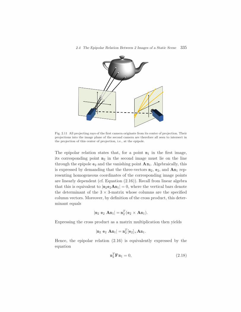
2.4 The Epipolar Relation Between 2 Images of a Static Scene 335
Fig. 2.11 All projecting rays of the first camera originate from its center of projection. Theirprojections into the image plane of the second camera are therefore all seen to intersect inthe projection of this center of projection, i.e., at the epipole.
The epipolar relation states that, for a point m1 in the first image,its corresponding point m2 in the second image must lie on the linethrough the epipole e2 and the vanishing point Am1. Algebraically, thisis expressed by demanding that the three-vectors m2, e2, and Am1 rep-resenting homogeneous coordinates of the corresponding image pointsare linearly dependent (cf. Equation (2.16)). Recall from linear algebrathat this is equivalent to |m2e2Am1| = 0, where the vertical bars denotethe determinant of the 3 × 3-matrix whose columns are the specifiedcolumn vectors. Moreover, by definition of the cross product, this deter-minant equals
|m2 e2 Am1| = mT2 (e2 × Am1).
Expressing the cross product as a matrix multiplication then yields
|m2 e2 Am1| = mT2 [e2]×Am1.
Hence, the epipolar relation (2.16) is equivalently expressed by theequation
mT2 Fm1 = 0, (2.18)

336 Principles of Passive 3D Reconstruction
where F = [e2]×A is a 3 × 3-matrix, called the fundamental matrix ofthe image pair, and with e2 the epipole in the second image and A theinvertible 3 × 3-matrix defined above [2, 4]. Note that, since [a]× is arank 2 matrix, the fundamental matrix F also has rank 2.
2.4.2 Gymnastics with F
The closed form (2.18) of the epipolar relation has the followingadvantages:
(1) The fundamental matrix F can, up to a non-zero scalar fac-tor, be computed from the image data alone.Indeed, for each pair of corresponding points m1 and m2 inthe images, Equation (2.18) yields one homogeneous linearequation in the entries of the fundamental matrix F. Know-ing (at least) eight pairs of corresponding point between thetwo images, the fundamental matrix F can, up to a non-zeroscalar factor, be computed from these point correspondencesin a linear manner. Moreover, by also exploiting the fact thatF has rank 2, the fundamental matrix F can even be com-puted, up to a non-zero scalar factor, from 7 point correspon-dences between the images, albeit by a non-linear algorithmas the rank 2 condition involves a relation between prod-ucts of three entries of F. Different methods for efficient androbust computation of F will be explained in Section 4.2.2 ofSection 4.
(2) Given F, the epipole e2 in the second image is the uniquethree-vector with third coordinate equal to 1, satisfyingFTe2 = 0.
This observation follows immediately from the fact thatF = [e2]×A and that [e2]T×e2 = −[e2]×e2 = −e2 × e2 = 0.
(3) Similarly, the epipole e1 of the second camera in the firstimage — i.e., the projection e1 of the position C2 of the sec-ond camera in the first image — is the unique three-vectorwith third coordinate equal to 1, satisfying Fe1 = 0.According to Equation (2.6) in Section 2.2.4, the pro-jection e1 of the position C2 of the second camera in

2.4 The Epipolar Relation Between 2 Images of a Static Scene 337
the first image is given by ρe1e1 = K1RT1 (C2 − C1), with
ρe1 a non-zero scalar factor. Since A = K2RT2 R1K−1
1 ,ρe1Ae1 = K2RT
2 (C2 − C1) = −ρe2e2, and thus ρe1Fe1 =[e2]× (ρe1Ae1) = [e2]×(−ρe2e2) = 0. Notice that this alsoshows that the infinite homography A maps the epipole e1
in the first image onto the epipole e2 in the second image.(4) Given a point m1 in the first image, the three-vector Fm1
yields homogeneous coordinates for the epipolar line 2 inthe second image corresponding to m1; i.e., 2 Fm1.Recall that the epipolar relation mT
2 Fm1 = 0 expresses thegeometrical observation that the point m2 in the secondimage, which corresponds to m1, lies on the line 2 throughthe epipole e2 and the point Am1, which by definition is theepipolar line in the second image corresponding to m1. Thisproves the claim.
(5) Similarly, given a point m2 in the second image, the three-vector FTm2 yields homogeneous coordinates for the epipolarline 1 in the first image corresponding to m2; i.e., 1 FTm2.By interchanging the role of the two images in the reasoningleading up to the epipolar relation derived above, one easilysees that the epipolar line 1 in the first image correspondingto a point m2 in the second image is the line through theepipole e1 in the first image and the vanishing point A−1m2
in the first image of the projecting ray of m2 in the secondcamera. The corresponding epipolar relation
|m1 e1 A−1m2| = 0 (2.19)
expresses that m1 lies on that line. As A is an invertiblematrix, its determinant |A| is a non-zero scalar. Multiply-ing the left-hand side of Equation (2.19) with |A| yields
|A||m1 e1 A−1m2| = |Am1 Ae1 m2|= |Am1 − (ρe2/ρe1)e2 m2|=
ρe2
ρe1|m2 e2 Am1| =
ρe2
ρe1mT
2 Fm1,

338 Principles of Passive 3D Reconstruction
because ρe1Ae1 = −ρe2e2, as seen in number 3 above, and|m2 e2 Am1| = mT
2 (e2 × Am1) = mT2 Fm1, by definition of the
fundamental matrix F (cf. Equation (2.18)). Consequently,the epipolar relation (2.19) is equivalent to mT
2 Fm1 = 0, andthe epipolar line 1 in the first image corresponding to agiven point m2 in the second image has homogeneous coor-dinates FTm2. We could have concluded this directly fromEquation 2.18 based on symmetry considerations.
2.4.3 Grasping the Infinite Homography
Before continuing our investigation on how to recover 3D informationabout the scene from images alone, it is worth to have a closer look atthe invertible matrix A introduced in Section 2.4.1 first. The matrix Ais defined algebraically as A = K2RT
2 R1K−11 , but it also has a clear
geometrical interpretation: the matrix A transfers vanishing points ofdirections in the scene from the first image to the second one. Indeed,consider a line L in the scene with direction vector V ∈ R
3. The van-ishing point v1 of its projection 1 in the first image is the point ofintersection of the line through the center of projection C1 and paral-lel to L with the image plane of the first camera, as depicted in Fig-ure 2.12. Parameter equations of this line are M = C1 + τ V with τ ascalar parameter, and the projection of every point M on this line inthe first image is given by K1RT
1 (X − C1) = τ K1RT1 V. The vanishing
L
C1
v1
image
l1
oo
Fig. 2.12 The vanishing point v1 in the first image of the projection 1 of a line L in thescene is the point of intersection of the line through the center of projection C1 and parallelto L with the image plane.

2.5 Two Image-Based 3D Reconstruction Up-Close 339
point v1 of the line 1 in the first image thus satisfies the equationρv1v1 = K1RT
1 V for some non-zero scalar ρv1. Similarly, the vanishingpoint v2 of the projection 2 of the line L in the second image is given byρv2v2 = K2RT
2 V for some non-zero scalar ρv2. Conversely, given a van-ishing point v1 in the first image, the corresponding direction vector Vin the scene is V = ρv1R1K−1
1 v1 for some scalar ρv1, and its vanishingpoint in the second image is given by ρv2v2 = ρv1K2RT
2 R1K−11 v1. As
A = K2RT2 R1K−1
1 , this relation between the vanishing points v1 andv2 can be simplified to ρv2 = Av1, where ρ = ρv2
ρv1is a non-zero scalar
factor. Hence, if v1 is the vanishing point of a line in the first image,then Av1 are homogeneous coordinates of the vanishing point of thecorresponding line in the second image, as was claimed. In particular,the observation made in Section 2.4.1 that for any point m1 in the firstimage Am1 are homogeneous coordinates for the vanishing point in thesecond view of the projecting ray of m1 in the first camera is in factanother instance of the same general property.
As is explained in more detail in Appendix A, in projective geom-etry, direction vectors V in the scene are represented as points on theplane at infinity of the scene. A vanishing point in an image then isjust the perspective projection onto the image plane of a point on theplane at infinity in the scene. In this respect, the matrix A is a homog-raphy matrix of the projective transformation that maps points fromthe first image via the plane at infinity of the scene into the secondimage. This explains why A is called the infinite homography in thecomputer vision literature.
2.5 Two Image-Based 3D Reconstruction Up-Close
From an algebraic point of view, triangulation can be interpreted assolving the two camera projection equations for the scene point M. For-mulated in this way, passive 3D reconstruction is seen as solving thefollowing problem: Given two images I1 and I2 of a static scene anda set of corresponding image points m1 ∈ I1 and m2 ∈ I2 between theseimages, determine a calibration matrix K1, a position C1 and an orien-tation R1 for the first camera and a calibration matrix K2, a positionC2 and an orientation R2 for the second camera, and for every pair of

340 Principles of Passive 3D Reconstruction
corresponding image points m1 ∈ I1 and m2 ∈ I2 compute world coordi-nates (X,Y,Z) of a scene point M such that:
ρ1m1 = K1RT1 (M − C1) and ρ2m2 = K2RT
2 (M − C2). (2.20)
These equations are the point of departure for our further analysis. Intraditional stereo one would know K1, R1, C1, K2, R2, and C2. Thenformula (2.20) yields a system of six linear equations in five unknownsfrom which the coordinates of M as well as the scalar factors ρ1 and ρ2
can be computed, as was explained in Section 2.3.Here, however, we are interested in the question which information
can be salvaged in cases where our knowledge about the camera con-figuration is incomplete. In the following sections, we will graduallyassume less and less information about the camera parameters to beknown. For each case, we will examine the damage to the precision withwhich we can still reconstruct the 3D structure of the scene. As willbe seen, depending on what is still known about the camera setup, thegeometric uncertainty about the 3D reconstruction can range from aEuclidean motion up to a 3D projectivity.
2.5.1 Euclidean 3D Reconstruction
Let us first assume that we do not know about the camera positionsand orientations relative to the world coordinate frame, but that weonly know the position and orientation of the second camera relativeto (the camera-centered reference frame of) the first one. We will alsoassume that both cameras are internally calibrated so that the matricesK1 and K2 are known as well. This case is relevant when, e.g., using ahand-held stereo rig and taking a single stereo image pair.
A moment’s reflection shows that it is not possible to determinethe world coordinates of M from the images in this case. Indeed, chang-ing the position and orientation of the world frame does not alter thesetup of the cameras in the scene, and consequently, does not alter theimages. Thus it is impossible to recover absolute information aboutthe cameras’ external parameters in the real world from the projectionEquation (2.20) alone, beyond what we already know (relative camerapose). Put differently, one cannot hope for more than to recover the

2.5 Two Image-Based 3D Reconstruction Up-Close 341
3D structure of the scene up to a 3D Euclidean transformation of thescene from the projection Equation (2.20) alone.
On the other hand, the factor RT1 (M − C1) in the right-hand side of
the first projection equation in formula (2.20) is just a Euclidean trans-formation of the scene. Thus, without loss of generality, we may replacethis factor by M′, because we just lost all hope of retrieving the 3D coor-dinates of M more precisely than up to some unknown 3D Euclideantransformation anyway. The first projection equation then simplifies toρ1m1 = K1M′. Solving M′ = RT
1 (M − C1 ) for M gives M = R1M′ + C1, andsubstituting this into the second projection equation in (2.20) yieldsρ2m2 = K2RT
2 R1M′ + K2RT2 (C1 − C2). Together,
ρ1m1 = K1M′ and ρ2m2 = K2RT
2 R1M′ + K2RT
2 (C1 − C2) (2.21)
constitute a system of equations which allow to recover the 3D structureof the scene up to a 3D Euclidean transformation M′ = RT
1 (M − C1).Indeed, as the cameras are assumed to be internally calibrated, K1 andK2 are known and the first equation in (2.21) can be solved for M′, viz.M′ = ρ1K−1
1 m1. Plugging this new expression for M′ into the right-handside of the second equation in formula (2.21), one gets
ρ2m2 = ρ1K2RT2 R1K−1
1 m1 + K2RT2 (C1 − C2). (2.22)
Notice that this actually brings us back to the epipolar relation (2.16)which was derived in Section 2.4.1. In this equation RT
2 R1 andRT
2 (C1 − C2) represent, respectively, the relative orientation and therelative position of the first camera with respect to the second one. Asthese are assumed to be known too, Equation (2.22) yields a systemof three linear equations from which the two unknown scalar factorsρ1 and ρ2 can be computed. And, when ρ1 is found, the Euclideantransformation M′ of the scene point M is found as well.
In summary, if the cameras are internally calibrated and the rela-tive position and orientation of the cameras is known, then for eachpair of corresponding points m1 and m2 in the images the Euclideantransformation M′ of the underlying scene point M can be recovered fromthe relations (2.21). Formula (2.21) is therefore referred to as a systemof Euclidean reconstruction equations for the scene and the 3D pointsM′ satisfying these equations constitute a Euclidean reconstruction of

342 Principles of Passive 3D Reconstruction
the scene. As a matter of fact, better than Euclidean reconstruction isoften not needed, as the 3D shape of the objects in the scene is per-fectly retrieved, only not their position relative to the world coordinateframe, which is completely irrelevant in many applications.
Notice how we have absorbed the unknown parameters into the newcoordinates M′. This is a strategy that will be used repeatedly in the nextsections. It is interesting to observe that M′ = RT
1 (M − C1) are, in fact,the coordinates of the scene point M with respect to the camera-centeredreference frame of the first camera, as was calculated in Section 2.2.4.The Euclidean reconstruction Equation (2.21) thus coincides with thesystem of projection Equation (2.20) if the world frame is the camera-centered reference frame of the first camera (i.e., C1 = 0 and R1 = I3)and the rotation matrix R2 then expresses the relative orientation ofthe second camera with respect to the first one.
2.5.2 Metric 3D Reconstruction
Next consider a stereo setup as that of the previous section, but sup-pose that we do not know the distance between the centers of projectionC1 and C2 any more. We do, however, still know the relative orienta-tion of the cameras and the direction along which the second camerais shifted with respect to the first one. This means that RT
2 (C1 − C2)is only known up to a non-zero scalar factor. As the cameras still areinternally calibrated, the calibration matrices K1 and K2 are knownand it follows that the last term in the second of the Euclidean recon-struction Equation (2.21), viz. K2RT
2 (C1 − C2), can only be deter-mined up to an unknown scalar factor. According to formula (2.15),K2RT
2 (C1 − C2) = ρe2e2 yields the epipole e2 of the first camera in thesecond image. Knowledge of the direction in which the second cam-era is shifted with respect to the first one, combined with knowledgeof K2, clearly also allows to determine e2. It is interesting to notice,however, that, if a sufficient of corresponding points can be foundbetween the images, then the fundamental matrix of the image paircan be computed, up to a non-zero scalar factor, and the epipole e2
can also be recovered that way (as explained in item 2 of Section 2.4.2and, in more detail, in Section 4). Having a sufficient number of point

2.5 Two Image-Based 3D Reconstruction Up-Close 343
correspondences would thus eliminate the need to know about the direc-tion of camera shift beforehand. On the other hand, the assumptionthat the inter-camera distance is not known implies that the scalarfactor ρe2 in the last term of the Euclidean reconstruction equations
ρ1m1 = K1M′ and ρ2m2 = K2RT
2 R1M′ + ρe2e2 (2.23)
is unknown. This should not come as a surprise, since ρe2 is theprojective depth of C1 in the second camera, and thus it is directlyrelated to the inter-camera distance. Algebraically, the six homoge-neous equations do not suffice to solve for the six unknowns M′, ρ1,ρ2, and ρe2. One only gets a solution up to an unknown scale. But,using the absorption trick again, we introduce the new coordinatesM = 1
ρe2M′ = 1
ρe2RT
1 (M − C1), which is a 3D similarity transformation ofthe original scene. Formulas (2.23) then reduces to
ρ1m1 = K1 M and ρ2m2 = K2RT2 R1 M + e2, (2.24)
where ρ1 = ρ1ρe2
and ρ2 = ρ2ρe2
are scalar factors expressing the projectivedepth of the scene point underlying m1 and m2 in each camera relative tothe scale ρe2 of the metric reconstruction of the scene. The coordinatesM provide a 3D reconstruction of the scene point M up to an unknown3D similarity, as expected.
We could have seen this additional scaling issue coming also intu-itively. If one were to scale a scene together with the cameras in it, thenthis would have no impact on the images. In terms of the relative cam-era positions, this would only change the distance between them, nottheir relative orientations or the relative direction in which one cam-era is displaced with respect to the other. The calibration matrices K1
and K2 would remain the same, since both the focal lengths and thepixel sizes are supposed to be scaled by the same factor and the num-ber of pixels in the image is kept the same as well, so that the offsetsin the calibration matrices do not change. Again, as such changes arenot discernible in the images, having internally calibrated cameras andexternal calibration only up to the exact distance between the cam-eras leaves us with one unknown, but fixed, scale factor. Together withthe unknown Euclidean motion already present in the 3D reconstruc-tion derived in the previous section, this unknown scaling brings the

344 Principles of Passive 3D Reconstruction
geometric uncertainty about the 3D scene up to an unknown 3D simi-larity transformation. Such a reconstruction of the scene is commonlyreferred to in the computer vision literature as a metric reconstructionof the scene, and formula (2.24) is referred to as a system of metricreconstruction equations. Although annoying, it should be noted thatfixing the overall unknown scale usually is the least of our worries inpractice, as indeed knowledge about a single distance or length in thescene suffices to lift the uncertainty about scale.
2.5.3 Affine 3D Reconstruction
A further step toward our goal of 3D reconstruction from the image dataalone is to give up on knowledge of the internal camera parameters aswell. For the metric reconstruction Equation (2.24) this implies thatthe calibration matrices K1 and K2 are also unknown. As before, onecan perform a change of coordinates M = K1 M and replace M in thereconstruction Equation (2.24) by M = K−1
1 M. This gives:
ρ1m1 = M and ρ2m2 = A M + e2, (2.25)
where ρ1 = ρ1, ρ2 = ρ2, and A = K2RT2 R1K−1
1 is the infinite homog-raphy introduced in Section 2.4.1. If the invertible matrix A is known,then this system (2.25) can be solved for the scalars ρ1, ρ2, and, moreimportantly, for M, as in the metric case (cf. Section 2.5.2). More onhow to extract A from image information only is to follow shortly. AsM = K1 M = 1
ρe2K1RT
1 (M − C1) represents a 3D affine transformation ofthe world space, formula (2.25) is referred to as a system of affine recon-struction equations for the scene and the 3D points M satisfying theseequations constitute an affine reconstruction of the scene, i.e., a recon-struction which is correct up to an unknown 3D affine transformation.
It suffices to know A and e2 in order to compute an affine recon-struction of the scene. As explained in Section 2.4.2 and in more detailin Section 4, e2 can be extracted from F, and F can be derived —up to a non-zero scalar factor — from corresponding points betweenthe images. Since e2 is in the left nullspace of F, an unknown scalarfactor on F does not prevent the extraction of e2, however. Unfortu-nately, determining A is not that easy in practice. A was defined as

2.5 Two Image-Based 3D Reconstruction Up-Close 345
A = K2RT2 R1K−1
1 , where K1 and K2 are the calibration matrices andRT
2 R1 represents the relative orientation of the cameras. If this infor-mation about the cameras is not available, then this formula cannot beused to compute A. On the other hand, the fundamental matrix F ofthe image pair has been defined in Section 2.4.1 as F = [e2]×A. But,unfortunately, the relation F = [e2]×A does not define the matrix Auniquely. Indeed, suppose A1 and A2 are 3 × 3-matrices such thatF = [e2]×A1 and F = [e2]×A2. Then [e2]×(A1 − A2) = 0. As [e2]×is the skew-symmetric 3 × 3-matrix which represents the cross prod-uct with the three-vector e2; i.e., [e2]×v = e2 × v for all v ∈ R
3, thecolumns of A1 and A2 can differ by a scalar multiple of e2. In par-ticular, A1 = A2 + e2aT for some three-vector a ∈ R
3. Hence, the infi-nite homography A cannot be recovered from point correspondencesbetween the images alone.
So, what other image information can then be used to determineA? Recall from Section 2.4.3 that the matrix A transfers vanishingpoints of directions in the scene from the first image to the second one.Each pair of corresponding vanishing points in the images thereforeyields constraints on the infinite homography A. More precisely, if v1
and v2 are the vanishing points in, respectively, the first and the sec-ond image of a particular direction in the scene, then ρv2 = Av1 forsome non-zero scalar factor ρ. Since A is a 3 × 3-matrix and each suchconstraint brings three equations, but also one additional unknown ρ,at least four such constraints are needed to determine the matrix A upto a scalar factor ρA. This unknown factor does not form an obstaclefor the obtained matrix to be used in the affine reconstruction Equa-tion (2.25), because by multiplying the first reconstruction equationwith the same factor and then absorbing it into M in the right-handside of both equations, one still obtains an affine 3D reconstruction ofthe scene.
Identifying the vanishing points of four independent directions in animage pair is rarely possible. More often, one has three dominant direc-tions, typically orthogonal to each other. This is the case for many built-up environments. Fortunately, there is one direction which is alwaysavailable, namely the line passing through the positions C1 and C2
in the scene. The vanishing points of this line in the images are the

346 Principles of Passive 3D Reconstruction
intersection of the line with each image plane. But these are just theepipoles. So, the epipoles e1 and e2 in a pair of images are correspond-ing vanishing points of the direction of the line through the camerapositions C1 and C2 in the scene and therefore satisfy the relation
ρee2 = Ae1 for some ρe ∈ R,
as we have already noted in Section 2.4.2, third item. Consequently, ifthe vanishing points of three independent directions in the scene can beidentified in the images, then the infinite homography A can be com-puted up to a non-zero scalar factor ; at least if none of the three direc-tions is that of the line connecting the centers of projection C1 and C2.
Notice that we have only absorbed K1 into the affine coordinates Mof the 3D reconstruction, but that K2 also can remain unknown, as itis absorbed by A.
2.5.4 Projective 3D Reconstruction
Finally, we have arrived at the situation where we assume no knowledgeabout the camera configuration or about the scene whatsoever. Instead,we only assume that one can find point correspondences between theimages and extract the fundamental matrix of the image pair.
The main conclusion of the previous section is that, if no informationabout the internal and external parameters of the camera is availableand if insufficient vanishing points can be found and matched, thenthe only factor that separates us from an affine 3D reconstruction ofthe scene is the infinite homography A. Let us therefore investigatewhether some partial knowledge about A can still be retrieved fromgeneral point correspondences between the images.
Recall from Section 2.4.1 that F = [e2]×A and that the epipole e2
can uniquely be determined from the fundamental matrix F. It is notdifficult to verify that ([e2]×)3 = −‖e2‖2 [e2 ]×, where ‖e2‖ denotes thenorm of the three-vector e2. As F = [e2]×A, it follows that
[e2]× ([e2]×F) = ([e2]×)3A = −‖e2‖2 [e2]× A = −‖e2‖2F.
So, [e2]×F is a 3 × 3-matrix which when premultiplied with [e2]×yields a non-zero scalar multiple of the fundamental matrix F. Inother words, up to a non-zero scalar factor, the 3 × 3-matrix [e2]×F

2.5 Two Image-Based 3D Reconstruction Up-Close 347
could be a candidate for the unknown matrix A. Unfortunately, asboth the fundamental matrix F and [e2]× have rank 2, the matrix[e2]×F is not invertible as A ought to be. But, recall from the pre-vious section that two matrices A1 and A2 satisfying F = [e2]×A1
and F = [e2]×A2 are related by A1 = A2 + e2aT for some three-vectora ∈ R
3. This implies that the unknown matrix A must be of the formA = −(1/‖e2‖2) [e2]×F + e2aT for some three-vector a ∈ R
3. It followsthat the invertible matrix A, needed for an affine reconstruction of thescene, can only be recovered up to three unknown components of a. Aswe do not know them, the simplest thing to do is to put them to zeroor to make a random guess. This section analyzes what happens to thereconstruction if we do just that.
The expression for A only takes on the particular form given abovein case F is obtained from camera calibration (i.e., from the rotationand calibration matrices). In case F is to be computed from pointcorrespondences — as is the case here — it can only be determinedup to a non-zero scalar factor. Let F be an estimate of the funda-mental matrix as obtained from point correspondences, then F = κ Ffor some non-zero scalar factor κ. Now define A = −(1/‖e2‖2) [e2]×F.Then A = κA + e2aT for some unknown three-vector a ∈ R
3. Noticethat, as observed before, the scalar factor κ between F and F has noinfluence on the pixel coordinates of e2, as derived from F instead of F.Using A for A in the affine reconstruction equations (2.25), for corre-sponding image points m1 and m2 we now solve the following system oflinear equations:
ρ1m1 = M and ρ2m2 = A M + e2, (2.26)
where ρ1 and ρ2 are non-zero scalar factors, and where the 3D pointsM constitute a 3D reconstruction of the scene, which — as will bedemonstrated next — differs from the original scene by a (unique, butunknown) 3D projective transformation. The set of 3D points M is calleda projective 3D reconstruction of the scene and formula (2.26) is referredto as a system of projective reconstruction equations. Figure 2.13 sum-marizes the steps that have lead up to these equations.
In order to prove that the points M obtained from Equation (2.26)do indeed constitute a projective 3D reconstruction of the scene,

348 Principles of Passive 3D Reconstruction
Projective 3D reconstruction from two uncalibrated images
Given: A set of point correspondences m1 ∈ I1 and m2 ∈ I2
between two uncalibrated images I1 and I2 of a static scene
Objective: A projective 3D reconstruction M of the scene
Algorithm:
(1) Compute an estimate F for the fundamental matrixa
(2) Computeb the epipole e2 from F(3) Compute the 3 × 3-matrix A = −(1/‖e2‖2) [e2]×F(4) For each pair of corresponding image points m1 and m2,
solve the following system of linear equations for M:
ρ1m1 = M and ρ2m2 = A M + e2
(ρ1 and ρ2 are non-zero scalars )
aCf. Section 2.4.2. See also Sections 4.2.2 and 4.2.3 in Section 4.bCf. Section 2.4.2. See also Section 4.3in Section 4.
Fig. 2.13 A basic algorithm for projective 3D reconstruction from two uncalibrated images.
we first express the Equation (2.26) in terms of projection matricesand extended coordinates
(M1
)= (X, Y , Z,1)T for the 3D point M =
(X, Y , Z)T (cf. formula (2.7) in Section 2.2.4):
ρ1m1 = (I3 | 0)(M
1
)and ρ2m2 = (A | e2)
(M
1
). (2.27)
Similarly, the affine reconstruction Equation (2.25) are written as:
ρ1m1 = (I3 | 0)(M
1
)and ρ2m2 = (A | e2)
(M
1
), (2.28)
where(M1
)= (X, Y , Z,1)T are the extended coordinates of the 3D point
M = (X, Y , Z)T . Recall that the invertible matrix A is of the form

2.5 Two Image-Based 3D Reconstruction Up-Close 349
A = κA + e2aT for some non-zero scalar κ and three-vector a ∈ R3.
The last equality in Equation (2.28) therefore is:
ρ2m2 = (κA + e2aT | e2)
(M
1
)= (A | e2)
(κI3 0
aT 1
)(M
1
); (2.29)
and the first equality in Equation (2.28) can be rewritten as:
κρ1m1 = (I3 | 0)(
κI3 0
aT 1
)(M
1
).
Comparing these expressions to formula (2.27), it follows that
λ
(M
1
)=
(κI3 0
aT 1
)(M
1
). (2.30)
for some non-zero scalar λ ∈ R and that ρ1 = (κ/λ) ρ1 and ρ2 =(1/λ) ρ2. Notice that one cannot simply go for a solution with λ = 1, asthis implies that aT = 0T and therefore A = κA. This would mean thatwe have been lucky enough to guess the correct infinite homographymatrix A (up to a scalar factor) right away. But this cannot be the caseaccording to our proposed choice : A has rank 2 and thus is singularwhereas the correct matrix A is invertible. Rather, eliminating λ fromEquation (2.30) gives:
M =κ M
aT M + 1.
Recall from Section 2.5.3 that M = 1ρe2
K1RT1 (M − C1). Substituting this
into the previous equation, one sees that
M =κK1RT
1 (M − C1)aT K1RT
1 (M − C1) + ρe2
is a projective transformation of the scene. Moreover, since M = K1 M
with M = 1ρe2
RT1 (M − C1) being the metric reconstruction of the scene
defined in Section 2.5.2, formula (2.30) can also be written as:
λ
(M
1
)=
(κK1 0
aTK1 1
)(M
1
); (2.31)

350 Principles of Passive 3D Reconstruction
or, after elimination of λ,
M =κK1 M
aT K1 M + 1,
which shows that M also is a projective transformation of M.
2.5.5 Taking Stock — Stratification
The goal put forward at the beginning of Section 2.5 was to recoverthe 3D geometrical structure of a scene from two images of it, with-out necessarily having complete information about the internal andexternal parameters of the cameras. It was immediately seen thatone can only recover it up to a 3D Euclidean transformation if onlyinformation about the relative camera poses is available for the exter-nal camera parameters. If the precise inter-camera distance is alsounknown, 3D reconstruction is only possible up to a 3D similarity andthe 3D reconstruction is said to be metric. Moreover, if the calibra-tion matrix of the first camera is unknown (and also of the secondcamera for that matter), then at most an affine 3D reconstruction ofthe scene is feasible. And, if the infinite homography A introduced inSection 2.4.1 is unknown, then the scene can only be reconstructed upto a 3D projective transformation. The latter case is very relevant, asit applies to situations where the internal and external parameters ofthe camera pair are unknown, but where point correspondences can befound.
Figure 2.14 illustrates these different situations. In the figure thescene consists of a cube. In a metric reconstruction a cube is found, butthe actual size of the cube is undetermined. In an affine reconstructionthe original cube is reconstructed as a parallelepiped. Affine transfor-mations preserve parallelism, but they do not preserve metric relationssuch as angles and relative lengths. In a projective reconstruction thescene appears as an (irregular) hexahedron, because projective trans-formations only preserve incidence relations such as collinearity andcoplanarity, but parallelism or any metric information is not preserved.Table 2.1 shows the mathematical expressions that constitute these geo-metrical transformations. The mutual relations between the differenttypes of 3D reconstruction are often referred to as stratification of the

2.5 Two Image-Based 3D Reconstruction Up-Close 351
ProjectiveAffine
Metric
similarity
OriginalEuclidean
Fig. 2.14 The aim of passive 3D reconstruction is to recover the 3D geometrical structureof the scene from images. With a fully calibrated setup of two cameras a Euclidean recon-struction can be achieved. The reconstruction degenerates to metric if the inter-cameradistance (sometimes referred to as baseline) is unknown. If the calibration matrices of thecameras are unknown, then the scene structure can only be recovered up to a 3D affinetransformation; and, if no information about the camera setup is available, then only aprojective reconstruction is feasible.
Table 2.1. The stratification of geometries.
Geometrical transf. Mathematical expression
Euclidean transf. M′ = RM + T with R a rotation matrix, T ∈ R3
similarity transform. M′ = κRM + T with R a rotation matrix, T ∈ R3, κ ∈ R
affine transf. M′ = QM + T with Q an invertible matrix, T ∈ R3
projective transf.
X′ = p11X+p12Y +p13Z+p14p41X+p42Y +p43Z+p44
Y ′ = p21X+p22Y +p23Z+p24p41X+p42Y +p43Z+p44
Z′ = p31X+p32Y +p33Z+p34p41X+p42Y +p43Z+p44
with P = (pij) an invertible 4 × 4-matrix
geometries. This term reflects that the transformations higher up in thelist are special types (subgroups) of the transformations lower down.Obviously, the uncertainty about the reconstruction increases whengoing down the list, as also corroborated by the number of degrees offreedom in these transformations.
In the first instance, the conclusion of this section — namely thatwithout additional information about the (internal and external) cam-era parameters the three-dimensional structure of the scene only canbe recovered from two images up to an unknown projective transforma-tion — might come as a disappointment. From a mathematical pointof view, however, this should not come as a surprise, because alge-braically passive 3D reconstruction boils down to solving the recon-struction Equations (2.20) for the camera parameters and the scene

352 Principles of Passive 3D Reconstruction
points M. In terms of projection matrices and extended coordinates(cf. formula (2.7) in Section 2.2.4), the reconstruction Equations (2.20)are formulated as:
ρ1m1 = P1
(M
1
)and ρ2m2 = P2
(M
1
), (2.32)
where Pj = (KjRTj | −KjRT
j Cj) is the 3 × 4-projection matrix of thej-th camera, with j = 1 or j = 2, and
(M1
)= (X,Y,Z,1)T are the
extended coordinates of the scene point M = (X,Y,Z)T . Moreover, itwas observed in Section 2.2.4 that in the general linear camera modelany 3 × 4-matrix of maximal rank can be interpreted as the projectionmatrix of a linear pinhole camera. Consequently, inserting an arbitraryinvertible 4 × 4-matrix and its inverse in the right-hand sides of theprojection Equations (2.32) does not alter the image points m1 and m2
in the left-hand sides of the equations and yields another — but equallyvalid — decomposition of the reconstruction equations:
ρ1m1 = P1H−1H(M
1
)and ρ2m2 = P2H−1H
(M
1
);
or equivalently,
ρ1m1 = P1
(M
1
)and ρ2m2 = P2
(M
1
), (2.33)
with P1 = P1H−1 and P2 = P2H−1 two 3 × 4-matrices of maximalrank, λ
(M1
)= H
(M1
)with λ a non-zero scalar a 3D projective transfor-
mation of the scene, and ρ1 = ρ1λ and ρ2 = ρ2
λ non-zero scalar factors.Clearly, formulas (2.33) can be interpreted as the projection equationsof scene points M that, when observed by cameras with respective pro-jection matrices P1and P2, yield the same set of image points m1 and m2.As H can be any invertible 4 × 4-matrix, it is clear that one cannothope to do better than recovering the 3D geometric structure of thescene up to an arbitrary 3D projective transformation if no informationabout the cameras is available. But, the longer analysis presented in theprevious sections and leading up to the same conclusion has providedan explicit algorithm for projective 3D reconstruction, which will berefined in the next sections.

2.6 From Projective to Metric Using More Than Two Images 353
Awareness of the stratification is also useful when additional infor-mation on the scene (rather than the cameras) is available. One mayknow some (relative) lengths or angles (including orthogonalities andparallelisms). Exploiting such information can make it possible toupgrade the geometric structure of the reconstruction to one with lessuncertainty, i.e., to one higher up in the stratification table. Basedon known lengths and angles, it may, for instance, become possibleto construct a 3D projective transformation matrix (homography) Hthat converts the projective reconstruction M, obtained from the imagedata (cf. Figure 2.13 and Equation (2.31) ), directly into a Euclideanone. And, even if no metric information about the scene is available,other geometrical relations that are known to exist in the scene maybe useful. In particular, we have already discussed the case of parallellines in three independent directions, that suffice to upgrade a pro-jective reconstruction into an affine one through the three vanishingpoints they deliver. Indeed, they allow to determine the three unknownparameters a ∈ R
3 of the invertible matrix A (cf. Section 2.5.3). Know-ing a allows to upgrade the projective 3D reconstruction M to the affine3D reconstruction κ M by using Equation (2.30) in Section 2.5.4. How-ever, one does not always need the projections of (at least) two parallellines in the image to compute a vanishing point. Alternatively, if in animage three points can be identified that are the projections of collinearscene points M1, M2, and M3 of which the ratio d(M1,M2)
d(M1,M3) of their Euclideandistances in the real world is known (e.g., three equidistant points inthe scene), then one can determine the vanishing point of this directionin the image using the cross ratio (cf. Appendix A). In Section 4.6.1of Section 4 such possibilities for improving the 3D reconstruction willbe explored further. In the next section, however, we will assume thatno information about the scene is available and we will investigatehow more than two images can contribute to better than a projective3D reconstruction.
2.6 From Projective to Metric Using More Than TwoImages
In the geometric stratification of the previous section, we ended upwith a 3D projective reconstruction in case no prior camera calibration

354 Principles of Passive 3D Reconstruction
information is available whatsoever and we have to work purely fromimage correspondences. In this section we will investigate how and whenwe can work our way up to a metric 3D reconstruction, if we were tohave more than just two uncalibrated images.
2.6.1 Projective Reconstruction and Projective CameraMatrices from Multiple Images
Suppose we are given m images I1, I2, . . . , Im of a static scene and a setof corresponding points mj ∈ Ij between the images (j ∈ 1,2, . . . ,m).As in formula (2.20) the projection equations of the j-th camera are:
ρj mj = Kj RTj (M − Cj) for j ∈ 1,2, . . . ,m; (2.34)
or, in terms of projection matrices and extended coordinates as in for-mula (2.32):
ρj mj =(KjRT
j | −KjRTj Cj
)(M1
)for j ∈ 1,2, . . . ,m. (2.35)
Of course, when one has more than just two views, one can stillextract at least a projective reconstruction of the scene, as when oneonly had two. Nonetheless, a note of caution is in place here. If we wereto try and build a projective reconstruction by pairing the first witheach of the other images separately and then combine the resultingprojective reconstructions, this would in general not work. Indeed, onehas to ensure that the same projective distortion is obtained for eachof the reconstructions. That this will not automatically amount from apairwise reconstruct-and-then-combine procedure becomes clear if onewrites down the formulas explicitly. When the internal and externalparameters of the cameras are unknown, a projective 3D reconstruc-tion of the scene can be computed from the first two images by theprocedure of Figure 2.13 in section 2.5.4. In particular, for each pointcorrespondence m1 ∈ I1 and m2 ∈ I2 in the first two images, the recon-structed 3D point M is the solution of the system of linear equations:
ρ1m1 = M and ρ2m2 = A2 M + e2, (2.36)
where ρ1 and ρ2 are non-zero scalars (which depend on M and thus arealso unknown) and A2 = (−1/‖e2‖2) [e2]×F12 with F12 an estimate of

2.6 From Projective to Metric Using More Than Two Images 355
the fundamental matrix between the first two images as computed frompoint correspondences. The resulting points M constitute a 3D recon-struction of the scene which relates to the metric reconstruction M bythe projective transformation:
λ
(M
1
)=
(κK1 0
aT K1 1
)(M
1
), (2.37)
as was demonstrated in Section 2.5.4 (formula (2.31)). Let H be thehomography matrix in the right-hand side of formula (2.37), viz.:
H =
(κK1 0
aT K1 1
). (2.38)
For the other images a similar set of equations can be derived by pairingeach additional image with the first one. But, as mentioned before, onehas to be careful in order to end up with the same projective distortionalready resulting from the reconstruction based on the first two views.Indeed, for an additional image Ij with j ≥ 3, blindly applying the pro-cedure of Figure 2.13 in Section 2.5.4 to the first and the j-th imageswithout considering the second image or the already obtained projec-tively reconstructed 3D points M would indeed result in a 3D projectivereconstruction M(j), but one which relates to the metric reconstruction M
by the projective transformation:
λ
(M(j)1
)=
(κ(j)K1 0
aT(j)K1 1
)(M
1
),
in which the parameters κ(j) ∈ R and a(j) ∈ R3 are not related to the
parameters κ and a in the projective transformation (2.37) and thecorresponding homography matrix H in formula (2.38). A consistentprojective reconstruction implies that aT
(j)/κ(j) = aT /κ. So, when intro-ducing additional images Ij with j ≥ 3 into the reconstruction process,one cannot simply choose the matrix Aj for each new view indepen-dently, but one has to make sure that the linear system of reconstructionequations:
ρ1m1 = M
and ρj mj = Aj M + ej for j ∈ 2, . . . ,m (2.39)

356 Principles of Passive 3D Reconstruction
is consistent, i.e., that it is such that the solutions M satisfy all recon-struction equations at once, in as far as image projections mj are avail-able. The correct way to proceed for the j-th image with j ≥ 3 thereforeis to express Aj more generally as Aj = κj (−1/‖ej ‖2) [ej ]×F1j + ej aT
j
where κj ∈ R and aj ∈ R3 are parameters such that the reconstruc-
tion equations ρj mj = Aj M + ej hold for all reconstructed 3D points Mobtained from Equations (2.36). Each image point mj brings three linearequations for the unknown parameters κj and aj , but also introduces1 unknown scalar factor ρj . Hence, theoretically 2 point correspon-dences between the first, the second and the j-th image would sufficeto determine κj and aj in a linear manner. However, the parameter-ization of the matrix Aj relies on the availability of the fundamentalmatrix F1j between the first and the j-th image. But, as explainedin Section 2.4.2, if F1j is to be estimated from point correspondencestoo, then at least 7 point correspondences are needed. Therefore, froma computational point of view it is better to estimate both A ande3 from the relation ρj mj = Aj M + ej directly. Indeed, for each imagepoint mj this formula yields three linear equations in the nine unknownentries of the matrix Aj and the two unknown pixel coordinates of theepipole ej , but it also introduces one unknown scalar factor ρj . Conse-quently, at least 6 point correspondences are needed to uniquely deter-mine Aj and ej in a linear manner. Moreover, since the fundamentalmatrix between the first and the j-th image is defined in Section 2.4.1as F1j = [ej ]×Aj , an estimate for Aj and ej immediately implies anestimate for F1j as well. At first sight this may seem a better approachto estimate the fundamental matrix F1j , because it only needs 6 pointcorrespondences instead of 7, but one should realize that three imagesare involved here (instead of only two images in Section 2.4.2). Therelations between three or more views of a static scene will be furtherexplored in Section 3. More information on how to efficiently computeAj in practice can be found in Section 4.4 of Section 4.
2.6.2 From Projective to Affine 3D Reconstruction
Now that the discussion of projective reconstruction is extended to thecase of more than two cameras, we next consider options to go beyond

2.6 From Projective to Metric Using More Than Two Images 357
this and upgrade to an affine or even a metric reconstruction. Butbefore doing so, we first make explicit the link between the plane atinfinity of the scene and the projective transformation matrix:
H =(
κK1 0
aTK1 1
), (2.40)
which describes the transition from a metric to a projective reconstruc-tion. Readers who are not very familiar with projective geometry canfind in Appendix A all necessary background material that is used inthis section, or they may skip this section and continue immediatelywith Section 2.6.3.
Recall that in projective geometry direction vectors are representedas points on the plane at infinity of the world space. If we would be ableto identify the plane at infinity of the scene in the projective reconstruc-tion, then by moving it to infinity, we can already upgrade the projec-tive reconstruction to an affine one. In the projective reconstruction M ofSection 2.6.1, the plane at infinity of the scene is found as the plane withequation aT M − κ = 0. Indeed, as explained in Appendix A, the planeat infinity of the scene has homogeneous coordinates (0,0,0,1)T in theworld space. Moreover, if a projective transformation whose action onhomogeneous coordinates of 3D points is represented by an invertible4 × 4-homography matrix H is applied to the world space, then homo-geneous coordinates of planes are transformed by the inverse transposeH−T = (H−1)T = (HT )−1 of the homography matrix P. For example,the 3D similarity transformation M = 1
ρe2RT
1 (M − C1) is represented inmatrix notation by:(
M
1
)=
( 1ρe2
RT1 − 1
ρe2RT
1 C1
0T 1
)(M
1
).
The corresponding homography matrix is: 1
ρe2RT
1 − 1ρe2
RT1 C1
0T 1
and its inverse transpose is:(ρe2RT
1 0
CT1 1
).

358 Principles of Passive 3D Reconstruction
The plane at infinity of the scene has homogeneous coordinates(0,0,0,1)T and is mapped by this similarity transformation onto itself,because
(ρe2RT
1 0
CT1 1
)0001
=
0001
.
This illustrates again the general fact that Euclidean, similarly andaffine transformations of the world space do not affect the plane atinfinity of the scene. A projective transformation on the contrary gen-erally does affect the plane at infinity. In particular, the projectivetransformation λ
(M1
)= H
(M1
)defined by the homography matrix (2.40)
maps the plane at infinity of the scene to the plane with homogeneouscoordinates:
H−T
0001
=
( 1κ K−T
1 − 1κ a
0T 1
)0001
=
(− 1
κ a
1
).
In other words, the plane at infinity of the scene is found in theprojective reconstruction M as the plane with equation − 1
κ aT M + 1 = 0,
or equivalently, aT M − κ = 0. Given this geometric interpretation of1κ a, it becomes even clearer why we need to keep these values thesame for the different choices of Aj in the foregoing discussion aboutbuilding a consistent, multi-view projective reconstruction of the scene.All two-view projective reconstructions need to share the same planeat infinity for them to be consistent. This said, even if one keeps the3D reconstruction consistent following the aforementioned method,one still does not know H or 1
κ aT .
If the position of the plane at infinity of the scene were known in theprojective reconstruction, one could derive a projective transformationwhich will turn the projective reconstruction into an affine one, i.e., toput the plane at infinity really at infinity. Indeed, Equation (2.37) can

2.6 From Projective to Metric Using More Than Two Images 359
be rewritten as:
λ
(M
1
)=
(κK1 0
aT K1 1
)(M
1
)=
(κI3 0
aT 1
)(K1 M
1
)
=
(κI3 0
aT 1
)(M
1
),
where M = K1 M is the affine 3D reconstruction that was introducedin section 2.5.3 (cf. formula (2.30) in section 2.5.4 ). Knowing that− 1
κ aT M + 1 = 0 is the equation of the plane at infinity of the scene
in the projective reconstruction, the previous equation can also bewritten as:
λ
(M
1
)=
(κI3 0
aT 1
)(M
1
)=
(I3 0
1κ a
T 1
)(κ M
1
). (2.41)
Observe that since M is an affine 3D reconstruction of the scene, κ M isan affine 3D reconstruction as well. Denoting π∞ = − 1
κ a, the plane atinfinity has equation πT∞ M + 1 = 0 and Equation (2.41) reads as:
λ
(M
1
)=
(I3 0
−πT∞ 1
)(κ M
1
).
This is the 3D projective transformation which maps the plane atinfinity in the affine reconstruction κ M to the plane with equationπT∞ M + 1 = 0 in the projective 3D reconstruction M. Put differently,if the plane at infinity of the scene can be identified as the planeπT∞ M + 1 = 0 in the projective reconstruction M (e.g., from directionswhich are known to be parallel in the scene or from vanishing pointsin the images), then the inverse projective transformation:
λ
(κM
1
)=
(I3 0
πT∞ 1
)(M
1
)with λ a non-zero scalar, (2.42)
or equivalently,
κ M =M
π∞T M + 1
turns the projective 3D reconstruction M into the affine reconstruc-tion κ M. In mathematical parlance, the projective transformation (2.42)maps the plane πT∞ M + 1 = 0 to infinity.

360 Principles of Passive 3D Reconstruction
2.6.3 Recovering Metric Structure : Self-CalibrationEquations
If no information is available about where the plane at infinity is locatedin the projective reconstruction M, one can still upgrade the reconstruc-tion, even to metric. Recall from formulas (2.39) that ρj mj = Aj M + ej
for all j ≥ 2 and from Equation (2.37) that:
λ
(M
1
)=
(κK1 0
aT K1 1
)(M
1
).
Together, these equations yield
ρj mj = Aj M + ej = (Aj | ej)(M
1
)
=1λ
(Aj | ej)
(κK1 0
aT K1 1
)(M
1
)
=1λ
(κAj K1 + ej aT K1 ej
)(M1
)
or equivalently,
λρj mj = (κAj K1 + ej aT K1) M + ej for all j ≥ 2.
On the other hand, a similar computation as in the derivation of themetric reconstruction Equations (2.24) in Section 2.5.2 shows that
ρj mj = Kj RTj R1 M + ej , with ρj =
ρj
ρej.
Comparing both equations, one sees that
κAj K1 + ej aT K1 = λj Kj RT
j R1 for all j ≥ 2
and for some scalar λj . In Section 2.6.2 it is observed that the param-eters κ ∈ R and a ∈ R
3 determine the plane at infinity of the scene inthe projective reconstruction: π∞ = − 1
κ a. Making this reference to theplane at infinity of the scene explicit in the previous equation, one gets
κj(Aj − ej πT∞)K1 = Kj RT
j R1 for all j ≥ 2, (2.43)

2.6 From Projective to Metric Using More Than Two Images 361
where κj = κ/λj is a non-zero scalar. This equation has two interestingconsequences. First of all, multiplying both sides of the equality on theright with the inverse of the calibration matrix K1 gives
κj(Aj − ej πT∞) = Kj RT
j R1K−11 for all j ≥ 2,
which, since the right-hand side of this equation is just the invertiblematrix Aj defined in Section 2.4.1, yields an explicit relation betweenthe infinite homography Aj and the 3 × 3-matrices Aj computed fromthe images as described in section 2.6.1, viz
Aj = κj (Aj − ej πT∞) for all j ≥ 2 (2.44)
with non-zero scalars κj ∈ R. And secondly, multiplying both sides inequality (2.43) on the right with the inverse R−1
1 = RT1 of the rotation
matrix R1 gives
κj(Aj − ej πT∞)K1RT
1 = Kj RTj for all j ≥ 2.
If one now multiplies both sides of this last equation with its transpose,then
(Kj RTj )(Kj RT
j )T = κ2j (Aj − ej πT
∞)K1RT1 (K1RT
1 )T (Aj − ej πT∞)T
for all j ≥ 2, which by RTj = R−1
j reduces to
Kj KTj = κ2
j (Aj − ej πT∞)K1KT
1 (Aj − ej πT∞)T (2.45)
for all j ∈ 2, . . . ,m. Equations (2.45) are the so-called self-calibrationor autocalibration equations [8] and all self-calibration methods essen-tially are variations on solving these equations for the calibration matri-ces Kj and the three-vector π∞ locating the plane at infinity of thescene in the projective reconstruction. The various methods may differin the constraints or the assumptions on the calibration matrices theyemploy, however.
2.6.4 Scrutinizing the Self-Calibration Equations
The self-calibration Equations (2.45) have a simple geometric interpre-tation, which we will explore first before looking into ways for solvingthem. Readers who are merely interested in the practice of 3D recon-struction may skip this section and continue with Section 2.6.5.

362 Principles of Passive 3D Reconstruction
2.6.4.1 Metric Structure and the Preservation of Angles
In Section 2.5.2 it was observed that if one wants to reconstruct a scenefrom images only and if no absolute distance is given for any parts ofthe scene, then one can never hope to do better than a metric recon-struction, i.e., a 3D reconstruction which differs from the original sceneby an unknown 3D similarity transformation. Typical of a 3D simi-larity transformation is that all distances in the scene are scaled bya fixed scalar factor and that all angles are preserved. Moreover, fora projective 3D reconstruction of the scene to be a metric one, it isnecessary and sufficient that the angles of any triangle formed by threepoints in the reconstruction are equal to the corresponding angles in thetriangle formed by the original three scene points. The self-calibrationEquations (2.45) enforce this condition in the projective reconstructionat hand, as will be explained now.
Let M, P, and Q be three arbitrary points in the scene. The anglebetween the line segments [M,P] and [M,Q] in Euclidean three-space isfound as the angle between the three-vectors P − M and Q − M in R
3.This angle is uniquely defined by its cosine, which is given by the for-mula:
cos(P − M,Q − M) =〈P − M,Q − M〉
‖P − M‖‖Q − M‖ ,
where 〈P − M,Q − M〉 denotes the (standard) inner product; and, ‖P −M‖ =
√〈P − M,P − M〉 and ‖Q − M‖ =√〈Q − M,Q − M〉 are the norms
of the three-vectors P − M and Q − M in R3. Now, P − M is a direc-
tion vector for the line defined by the points M and P in the scene.As explained in Appendix A, the vanishing point vj of the line MP inthe j-th image (j ∈ 1,2, . . . ,m) is given by ρvj vj = Kj RT
j (P − M),where ρj mj = Kj RT
j (M − Cj) are the projection equations of the j-thcamera, as defined by formula (2.34). Since Rj is a rotation matrix,RT
j = R−1j and the three-vector P − M can (theoretically) be recovered
up to scale from its vanishing point vj in the j-th image by the for-mula P − M = ρvj Rj K−1
j vj . Similarly, Q − M is a direction vector of theline through the points M and Q in the scene and the vanishing pointwj of this line in the j-th image is given by ρwj wj = Kj RT
j (Q − M),thus yielding Q − M = ρwj Rj K−1
j wj . By definition of the inner

2.6 From Projective to Metric Using More Than Two Images 363
product in R3,
〈P − M,Q − M〉 = (P − M)T (Q − M)
= (ρvj Rj K−1j vj)T (ρwj Rj K−1
j wj)
= ρvj ρwj vTj K−T
j K−1j wj
= ρvj ρwj vTj (Kj KT
j )−1wj .
A similar calculation yields
‖P − M‖2 = (P − M)T (P − M) = ρ2vj vT
j (Kj KTj )−1vj
and ‖Q − M‖2 = (Q − M)T (Q − M) = ρ2wj wT
j (Kj KTj )−1wj .
Combining the previous expressions, one gets the following formula forthe cosine of the angle between the line segments [M,P] and [M,Q] in thescene:
cos(P − M,Q − M) =vT
j (Kj KTj )−1wj√
vTj (Kj KT
j )−1vj
√wT
j (Kj KTj )−1wj
. (2.46)
This equation states that the angle between two lines in the scene canbe measured from a perspective image of the scene if the vanishingpoints of these lines can be identified in the image and if the calibrationmatrix Kj of the camera — or rather Kj KT
j — is known.This should not come as a surprise, since vanishing points encode
3D directions in a perspective image. What is more interesting tonotice, however, is that the inner product of the scene is encoded inthe image by the symmetric matrix (Kj KT
j )−1. In the computer visionliterature this matrix is commonly denoted by ωj and referred to as theimage of the absolute conic in the j-th view [16]. We will not expand onthis interpretation right now, but the interested reader can find moredetails on this matter in Appendix B. The fact that the calibrationmatrix Kj appears in a formula relating measurements in the image tomeasurements in the scene was to be expected. The factor RT
j (M − Cj)in the right-hand side of the projection equations ρj mj = Kj RT
j (M − Cj)corresponds to a rigid motion of the scene, and hence does not have aninfluence on angles and distances in the scene. The calibration matrixKj , on the other hand, is an upper triangular matrix, and thus intro-duces scaling and skewing. When measuring scene angles and distances

364 Principles of Passive 3D Reconstruction
from the image, one therefore has to undo this skewing and scalingfirst by premultiplying the image coordinates with the inverse matrixK−1
j . And, last but not least, from the point of view of camera self-calibration, Equation (2.46) introduces additional constraints betweendifferent images of the same scene, viz.:
vTi (Ki KT
i )−1wi√vT
i (Ki KTi )−1vi
√wT
i (Ki KTi )−1wi
=vT
j (Kj KTj )−1wj√
vTj (Kj KT
j )−1vj
√wT
j (Kj KTj )−1wj
,
which must hold for every pair of images i, j ∈ 1,2, . . . ,m and forevery two pairs of corresponding vanishing points vi, vj and wi, wj inthese images. Obviously, only m − 1 of these relations are independent:
vT1 (K1 KT
1 )−1w1√
vT1 (K1 KT
1 )−1v1
√wT1 (K1 KT
1 )−1w1
=vT
j (Kj KTj )−1
wj√vT
j (Kj KTj )−1
vj
√wT
j (Kj KTj )−1
wj
(2.47)for every j ≥ 2 and for every two pairs of corresponding vanishingpoints v1, vj and w1, wj between the first and the j-th image. Theself-calibration Equations (2.45) enforce these constraints in the pro-jective reconstruction of the scene, as will be demonstrated next.
2.6.4.2 Infinity Homographies and thePreservation of Angles
To see why the final claim in the last section holds, we have to reinter-pret the underlying relation (2.46) in terms of projective geometry. Con-sider again the (arbitrary) scene points M, P, and Q. Their extended coor-dinates, respectively, are
(M1
),(P1
), and
(Q1
). As explained in Appendix A,
the direction vector P − M of the line L through the points M and P inthe scene corresponds in projective three-space to the point of inter-section of the line through the projective points
(M1
)and
(P1
)with the
plane at infinity of the scene; and the vanishing point vj of L in thej-th image is the perspective projection of this point of intersectiononto the image plane of the j-th camera (j ∈ 1,2, . . . ,m). In particu-lar, the vanishing points v1, v2, . . . , vm are corresponding points in theimages I1, I2, . . . , Im. Moreover, it was explained in Section 2.4.3 thatthe matrix Aj = Kj RT
j R1K−11 introduced in Section 2.4.1 actually is

2.6 From Projective to Metric Using More Than Two Images 365
a homography matrix representing the projective transformation thatmaps (vanishing) points from the first image via the plane at infinityof the scene onto the corresponding (vanishing) point in the j-th image(j ≥ 2), and therefore is referred to in the computer vision literature asthe infinite homography between the first and the j-th image. Explicitly,Aj v1 = ρj vj for some non-zero scalar factor ρj . Similarly, the vanishingpoints w1 and wj of the line through M and Q in, respectively, the firstand j-th image satisfy Aj w1 = σj wj for some non-zero scalar factor σj .Using the infinite homography Aj = Kj RT
j R1K−11 , the inner product
vTj (Kj KT
j )−1wj in the j-th image can also be expressed in terms of thecorresponding vanishing points v1 and w1 in the first image:
vTj (Kj KT
j )−1wj =(
1ρj
Aj v1
)T
(Kj KTj )−1
(1σj
Aj w1
)
=1ρj
1σj
vT1 AT
j (Kj KTj )−1Aj w1. (2.48)
Using again Aj = Kj RTj R1K−1
1 and the fact that RTj = R−1
j , since Rj
is a rotation matrix, the 3 × 3-matrix ATj (Kj KT
j )−1Aj in the right-hand side of the previous equality simplifies to:
ATj (Kj KT
j )−1Aj = (Kj RTj R1K−1
1 )T (K−Tj K−1
j )(Kj RTj R1K−1
1 )
= (K1KT1 )−1.
Equation (2.48) then reads
vT1 (K1KT
1 )−1w1 = ρj σjvTj (Kj KT
j )−1wj .
By similar calculations, one also finds that vT1 (K1KT
1 )−1v1 =ρ2
jvTj (Kj KT
j )−1vj and wT1 (K1KT
1 )−1w1 = σ2jw
Tj (Kj KT
j )−1wj . Together,these three equalities establish the relations (2.47) in an almost triv-ial manner. It is important to realize, however, that it actually is theequality:
ATj (Kj KT
j )−1Aj = (K1KT1 )−1, (2.49)
which makes that the constraints (2.47) are satisfied. Our claimis that the self-calibration Equations (2.45) are nothing else butthis fundamental relation (2.49) expressed in terms of the projective
366 Principles of Passive 3D Reconstruction
reconstruction of the scene which was computed from the given imagesas described in Section 2.6.1.
2.6.4.3 Equivalence of Self-Calibration and thePreservation of Angles
Now, suppose that no information whatsoever on the scene is given,but that we have computed matrices Aj and epipoles ej for each image(j ≥ 2) as well as a collection of 3D points M satisfying the projectivereconstruction Equations (2.39), viz.:
ρ1m1 = M and ρj mj = Aj M + ej for j ∈ 2, . . . ,m,
for given point correspondences m1,m2, . . . ,mm between the images. The3D points M have been shown in Section 2.5.4 to form a projective3D reconstruction of the scene. To prove our claim about the self-calibration equations, we will follow the same line of reasoning as theone that led to relation (2.49) above. Let M and P be two arbitrary pointsin the projective reconstruction. As explained in Appendix A, the van-ishing point vj in the j-th image of the line L through the points M andP in the 3D reconstruction is the projection of the point of intersectionof the line L with the plane at infinity of the scene. Since no informationwhatsoever on the scene is available, we do not know where the planeat infinity of the scene is located in the reconstruction. However, we doknow that for every 3D line in the projective reconstruction, its vanish-ing points in the respective images should be mapped onto each otherby the projective transformation which maps one image to another viathe plane at infinity of the scene. The idea now is to identify a plane inthe projective reconstruction which does exactly that. Suppose that the(unknown) equation of this plane is πT∞ M + 1 = 0. The projective trans-formation which maps the first image to the j-th one via this plane iscomputed as follows: From the first projective reconstruction equationρ1m1 = M it follows that parameter equations for the projecting ray ofan arbitrary image point m1 in the first camera are given by M = ρm1
where ρ ∈ R is a scalar parameter. This projecting ray intersects theplane at infinity of the scene in the point M∞ = ρ∞m1 that satifies the

2.6 From Projective to Metric Using More Than Two Images 367
equation πT∞ M∞ + 1 = 0. Hence,
ρ∞ = − 1πT∞m1
and M∞ = − 1πT∞m1
m1.
By the projective reconstruction Equations (2.39), the projection mj ofthis point M∞ in the j-th image for j ≥ 2 satisfies ρj mj = Aj M∞ + ej .Substituting the expression for M∞ in this equation yields
ρj mj = − 1πT∞m1
Aj m1 + ej ,
or equivalently,
−(πT∞m1)ρj mj = Aj m1 − ej(πT
∞m1) = (Aj − ej πT∞)m1.
Consequently, the 3 × 3-matrix Aj − ej πT∞ is a homography matrix ofthe projective transformation which maps the first image to the j-thone via the plane at infinity of the scene. In Section 2.4.3, on the otherhand, it was demonstrated that the invertible matrix Aj introduced inSection 2.4.1 also is a matrix for this infinite homography. Therefore,Aj − ej πT∞ and Aj must be equal up to a non-zero scalar factor, i.e.,Aj = κj (Aj − ej πT∞) for some non-zero scalar κj ∈ R. Notice that thisis exactly the same expression for Aj as was found in Equation (2.44) ofSection 2.6.3, but now it is obtained by a geometrical argument insteadof an algebraic one.
Clearly, for any plane πT M + 1 = 0 the homography matrix Aj −ej πT will map the first image to the j-th one via that plane. But onlythe plane at infinity of the scene will guarantee that the cosines
vT1 (K1KT
1 )−1w1√vT
1 (K1KT1 )−1v1
√wT
1 (K1KT1 )−1w1
andvT
j (Kj KTj )−1wj√
vTj (Kj KT
j )−1vj
√wT
j (Kj KTj )−1wj
(cf. Equation (2.47) ) computed in each image j (j ≥ 2) admit the samevalue whenever v1 is mapped onto vj and w1 is mapped onto wj by thehomography Aj − ej πT . And, as was observed earlier in this section,this will only be guaranteed if AT
j (Kj KTj )−1Aj = (K1KT
1 )−1 where

368 Principles of Passive 3D Reconstruction
Aj now has to be interpreted as the infinite homography mapping thefirst image to the j-th image by the plane at infinity of the scene (cf.Equation (2.49) ). Since Aj = κj (Aj − ej πT∞), the plane at infinity ofthe scene is that plane πT∞ M + 1 = 0 in the projective reconstructionfor which
κ2j (Aj − ej πT
∞)T (Kj KTj )−1(Aj − ej πT
∞) = (K1KT1 )−1
for all j ∈ 2,3, . . . ,m. This equality expresses that the intrinsic wayof measuring in the j-th image — represented by the symmetric matrix(Kj KT
j )−1 — must be compatible with the intrinsic way of mea-suring in the first image — represented by the symmetric matrix(K1KT
1 )−1 — and, more importantly, that it is the infinite homogra-phy between the first and the j-th image — represented by the matrix(Aj − ej πT∞ ) — which actually transforms the metric (Kj KT
j )−1 intothe metric (K1KT
1 )−1. Finally, if both sides of this matrix equality areinverted, one gets the relation:
1κ2
j
(Aj − ej πT∞)−1Kj KT
j (Aj − ej πT∞)−T = K1KT
1 ,
or, after solving for Kj KTj ,
Kj KTj = κ2
j (Aj − ej πT∞)K1KT
1 (Aj − ej πT∞)T , (2.50)
which must hold for all j ∈ 2,3, . . . ,m. Observe that these are exactlythe self-calibration Equations (2.45), as we claimed earlier.
Intuitively, these equations state that if a plane πT∞ M + 1 = 0 inthe reconstruction is known or found to be the plane at infinity of thescene and if a metric — represented by a symmetric, positive-definitematrix K1KT
1 — is induced in the first image, then by really map-ping the plane π∞ M + 1 = 0 to infinity and by measuring in the j-thimage (j ≥ 2) according to a metric induced from K1KT
1 through for-mula (2.50), the projective reconstruction will be upgraded to a metric3D reconstruction of the scene. This is in accordance with our findingsin Section 2.6.2 that the projective transformation:
κ M =K−1
1 M
πT∞ M + 1

2.6 From Projective to Metric Using More Than Two Images 369
transforms the projective reconstruction M into the metric reconstruc-tion κ M.
2.6.5 A Glimpse on Absolute Conics and Quadrics
The right-hand side of the self-calibration Equations (2.50) can also bewritten as:
Kj KTj = κ2
j (Aj − ej πT∞)K1KT
1 (Aj − ej πT∞)T
= κ2j
(Aj ej
)( I3
−πT∞
)K1KT
1(I3 −π∞
)(ATj
eTj
)
= κ2j
(Aj ej
)( K1KT1 −K1KT
1 π∞
−πT∞K1KT1 πT∞K1KT
1 π∞
)(AT
j
eTj
).
In the computer vision literature, the 3 × 3-matrix Kj KTj in the left-
hand side of the equality is commonly denoted by ω∗j and referred to
as the dual image of the absolute conic in the j-th view [16]. It is themathematical dual of the image of the absolute conic ωj in the j-thview. The 4 × 4-matrix
Ω∗ =
(K1KT
1 −K1KT1 π∞
−πT∞K1KT1 πT∞K1KT
1 π∞
)(2.51)
in the right-hand side of the previous equality, on the other hand, isin the computer vision literature usually referred to as the absolutequadric [16]. The self-calibration Equations (2.50) are compactly writ-ten in this manner as:
ω∗j = κ2
j (Aj | ej) Ω∗ (Aj | ej)T , (2.52)
where ω∗j = Kj KT
j and with Ω∗ as defined above. We will not expandon this interpretation in terms of projective geometry right now, but theinterested reader can find more details on this matter in Appendix B.
The main advantage of writing the self-calibration equations in theform (2.52) is that it yields linear equations in the entries of ω∗
j andthe entries of Ω∗, which are easier to solve in practice than the non-linear formulation (2.50). Moreover, the absolute quadric Ω∗ encodes

370 Principles of Passive 3D Reconstruction
both the plane at infinity of the scene and the internal calibration ofthe first camera in a very concise fashion. Indeed,
Ω∗ =
(I3 0
−πT∞ 1
)(K1KT
1 0
0T 0
)(I3 0
−πT∞ 1
)T
,
from which it immediately follows that Ω∗ has rank 3 and that itsnullspace is spanned by the plane at infinity of the scene (πT∞ 1)T . More-over, Ω∗ can also be decomposed as:
Ω∗ =
(K1 0
−πT∞K1 1
)(I3 0
0T 0
)(K1 0
−πT∞K1 1
)T
,
where the 4 × 4-matrix(K1 0
−πT∞K1 1
)=
(I3 0
−πT∞ 1
)(K1 0
0T 1
), (2.53)
is the homography matrix of the projective transformation
λ
(M
1
)=
(K1 0
−πT∞K1 1
)(κ M
1
),
which relates the projective reconstruction M to the metric reconstruc-tion κ M, as discussed in Section 2.6.2. Hence, the rectifying homogra-phy to update the projective reconstruction of the scene to a metricone is directly available once the absolute quadric Ω∗ has been recov-ered. It is interesting to observe that the decomposition (2.53) of therectifying homography exhibits the stratification of geometries as dis-cussed in Section 2.5.5. The rightmost matrix in the right-hand sideof Equation (2.53) represents the affine deformation induced on themetric reconstruction κ M by including the uncertainty about the inter-nal camera parameters K1 in the 3D reconstruction, yielding the affinereconstruction κ M; and the leftmost matrix in the decomposition (2.53)changes the plane at infinity to the plane πT∞ M + 1 = 0 in the projectivereconstruction M of the scene.
How Ω∗ is computed in practice, given a projective reconstructionof the scene is discussed in more detail in Section 4.6.2 of Section 4.Therefore we will not continue with this topic any further here, butinstead we will address the question of how many images are needed inorder for the self-calibration equations to yield a unique solution.

2.6 From Projective to Metric Using More Than Two Images 371
2.6.6 When do the Self-Calibration Equations Yield aUnique Solution ?
The self-calibration equations yield additional constraints on thecalibration matrices of the cameras and about the location of theplane at infinity of the scene in a projective 3D reconstruction. Butas was already observed in Sections 2.5.4 and 2.5.5, if no additionalinformation about the internal and/or external calibration of thecameras or about the Euclidean structure of the scene is available,then with only two images one cannot hope for better than a projectivereconstruction of the scene. The question that remains unsolved uptill now is: Is it possible to recover a metric reconstruction of the scenewith only the images at our disposal; and, more importantly, howmany images are needed to obtain a unique solution?
Consider again the self-calibration Equations (2.50) in their com-pact formulation:
Kj KTj = κ2
j (Aj − ej πT∞)K1KT
1 (Aj − ej πT∞)T (2.54)
for each j ∈ 2,3, . . . ,m. In these equations the calibration matrices Kj
all appear as Kj KTj . It is thus advantageous to take the entries of
Kj KTj as the unknowns in the self-calibration equations instead of
expressing them in terms of the internal camera parameters consti-tuting Kj (cf. formula (2.4)). As Kj is an invertible upper-triangularmatrix, Kj KT
j is a positive-definite symmetric matrix. So, if Kj KTj
is known, the calibration matrix Kj itself can uniquely be obtainedfrom Kj KT
j by Cholesky factorization [3]. Furthermore, each Kj KTj
is a symmetric 3 × 3-matrix whose (3,3)-th entry equals 1 (cf. for-mula (2.4)). Consequently, each Kj KT
j is completely characterizedby five scalar parameters, viz. the diagonal elements other than the(3,3)-th one and the upper-triangular entries. Similarly, the scalarfactors κ2
j can be considered as being single variables in the self-calibration equations. Together with the three unknown componentsof the three-vector π∞, the number of unknowns in the self-calibrationEquations (2.54) for m images add up to 5m + (m − 1) + 3 = 6m + 2.On the other hand, for m images, formula (2.54) yields m − 1 matrixequations. Since both sides of these equations are formed by symmetric

372 Principles of Passive 3D Reconstruction
3 × 3-matrices, each matrix equation induces only six different non-linear equations in the components of KjKT
j , the components of π∞and the scalars κ2
j for j ∈ 1,2, . . . ,m. Hence, for m images, the self-calibration Equations (2.54) yield a system of 6(m − 1) = 6m − 6non-linear equations in 6m + 2 unknowns. Clearly, without additionalconstraints on the unknowns, this system does not have a unique solu-tion.
In practical situations, however, quantitative or qualitative infor-mation about the cameras can be used to constrain the number ofsolutions. Let us consider some examples.
• Images obtained by the same or identical cameras.
If the images are obtained with one or more cameras whosecalibration matrices are the same, then K1 = K2 = . . . =Km = K and the self-calibration Equations (2.54) reduce to
KKT = κ2j (Aj − ej πT
∞)KKT (Aj − ej πT∞)T
for all j ∈ 2, . . . ,m. In this case, only five internal cam-era parameters — in practice, the five independent scalarscharacterizing KKT — are to be determined, reducing thenumber of unknowns to 5 + (m − 1) + 3 = m + 7. On theother hand, the self-calibration equations yield six equationsfor each image other than the first one. If these equationsare independent for each view, a solution is determinedprovided 6(m − 1) ≥ m + 7. Consequently, if m ≥ 3 imagesobtained by cameras with identical calibration matrices, thenthe calibration matrix K and the plane at infinity of thescene can — in principle — be determined from the self-calibrations equations and a metric reconstruction of thescene can be obtained.
• Images obtained by the same or identical cameraswith different focal lengths.
If only the focal length of the camera is varying between theimages, then four of the five internal parameters are the samefor all cameras, which brings the total number of unknownsto 4 + m + (m − 1) + 3 = 2m + 6. Since the self-calibration

2.6 From Projective to Metric Using More Than Two Images 373
Equations (2.54) bring six equations for each image otherthan the first one, a solution is in principle determined pro-vided 6(m − 1) ≥ 2m + 6. In other words, when the focallength of the camera is allowed to vary between the images,then — in principle — a metric reconstruction of the scenecan be obtained from m ≥ 3 images.
• Known aspect ratio and skew, but unknown and dif-ferent focal length and principal point.
When the aspect ratio and the skew of the cameras areknown, but the focal length and the principal point of thecameras are unknown and possibly different for each image,only three internal parameters have to be determined for eachcamera. This brings the number of unknowns for all m imagesto 3m + (m − 1) + 3 = 4m + 2. As formula (2.54) bringssix equations for each image other than the first one, a solu-tion is in principle determined provided 6(m − 1) ≥ 4m + 2.In other words, when the aspect ratio and the skew of the cam-eras are known, but the focal length and the principal pointof the cameras are unknown and allowed to vary between theimages, then — in principle — a metric reconstruction ofthe scene can be obtained from m ≥ 4 images. Note that thecase of square pixels, usual with digital cameras, is a specialcase of this.
• Rectangular pixels (and, hence, known skew) andunknown, but fixed aspect ratio.
In case the skew of the pixels is known and if the aspectratio is identical for all cameras, but unknown, then thetotal number of unknowns in the self-calibration equations is1 + 3m + (m − 1) + 3 = 4m + 3. Because there are six self-calibration equations for each image other than the first one,a solution is in principle determined provided 6(m − 1) ≥4m + 3. In other words, when the skew of the cameras isknown and if the aspect ratio is identical for all cameras, butunknown, and if the focal length and the principal point ofthe cameras are unknown and allowed to vary between the

374 Principles of Passive 3D Reconstruction
images, then — in principle — a metric reconstruction ofthe scene can be obtained from m ≥ 5 images.
• Aspect ratio and skew identical, but unknown.
In the situation where the aspect ratio and the skew of thecameras are identical, but unknown, two of the five inter-nal parameters are the same for all cameras, which bringsthe total number of unknowns to 2 + 3m + (m − 1) + 3 =4m + 4. As formula (2.54) brings six equations for eachimage other than the first one, a solution is in principle deter-mined provided 6(m − 1) ≥ 4m + 4. In other words, if theaspect ratio and the skew are the same for each camera, butunknown, and when the focal length and the principal point ofthe camera are allowed to vary between the images, then —in principle — a metric reconstruction of the scene can beobtained from m ≥ 5 images.
• Rectangular pixels or known skew.
If only the skew is known for each image, then four internalparameters have to be determined for each camera, whichbrings the total number of unknowns to 4m + (m − 1) + 3 =5m + 2. Since there are six self-calibration equations for eachimage other than the first one, a solution is in principle deter-mined provided 6(m − 1) ≥ 5m + 2. In other words, whenonly the skew is known for each image, but all the otherinternal parameters of the camera are unknown and allowedto vary between the images, then — in principle — a met-ric reconstruction of the scene can be obtained from m ≥ 8images.
• Aspect ratio unknown, but fixed.
When the aspect ratio of the pixels is the same for all cam-eras, but its value is unknown, then of the five unknowninternal parameters of the cameras, one is the same for allcameras, thus bringing the total number of unknowns to1 + 4m + (m − 1) + 3 = 5m + 3. With six self-calibrationequations for each image other than the first one, a solu-tion is in principle determined provided 6(m − 1) ≥ 5m + 3.

2.7 Some Important Special Cases 375
In other words, if the aspect ratio of the pixels is the samefor each camera, but its value is unknown, and when all theother internal parameters of the cameras are unknown andallowed to vary between the images, then — in principle —a metric reconstruction of the scene can be obtained fromm ≥ 9 images.
In conclusion, although the self-calibration Equations (2.54) bringtoo few equations to allow a unique solution for the calibrationmatrice Kj of each camera and to uniquely identify the plane at infin-ity of the scene in the projective 3D reconstruction, in most practicalsituations a unique solution can be obtained by exploiting additionalconstraints on the internal parameters of the cameras, provided a suffi-cient number of images are available. The required minimum number ofimages as given above for different situations only is indicative in thatit is correct, provided the resulting self-calibration equations are inde-pendent. In most applications this will be the case. However, one shouldalways keep in mind that there do exist camera configurations and cam-era motions for which the self-calibration equations become dependentand the system is degenerate. Such special situations are referred toin the literature as critical motion sequences. A detailed analysis of allthese cases is beyond the scope of this text, but the interested readeris referred to [9, 14, 15] for further information. Moreover, it must alsobe emphasized that the self-calibration equations in (2.54) are not verywell suited for numerical computations. For practical use, their linearformulation (2.52) in terms of the absolute quadric is recommended.Section 4.6.2 of Section 4 discusses this issue in more detail.
2.7 Some Important Special Cases
In the preceding sections the starting point was that no informationabout the internal and external parameters of the cameras was avail-able and that the positions and orientations of the cameras could becompletely arbitrary. In the last section, it was observed that one has toassume some constraints on the internal parameters in order to solve theself-calibration equations, thereby still leaving the external parameters

376 Principles of Passive 3D Reconstruction
completely unknown at the outset. In practical applications, the lat-ter might not always be the case either and quite a bit of knowledgeabout the camera motion may be available. Situations in which theobject or the camera has purely translated in between the acquisitionof the images are quite common (e.g., camera on rails), and so arecases of pure camera rotation (e.g., camera on tripod). These simplecamera motions both offer opportunities and limitations, which will beexplored in this section.
Moreover, sometimes it makes more sense to first calibrate camerasinternally, and then to only recover 3D structure and external param-eters from the images. An example is digital surveying (3D measuringin large-scale environments like cities) with one or more fixed camerasmounted on a van. These cameras can be internally calibrated beforedriving off for a new surveying campaign, during which the internalparameters can be expected to remain fixed.
And, last but not least, in practical applications it may often beuseful and important — apart from reconstructing the 3D structureof the scene — to obtain also information about the camera positionsand orientations or about the camera parameters underlying the imagedata. In the computer vision literature this is referred to as structure-and-motion. The 3D reconstruction process outlined in the previoussections can provide such information too. The fundamental conceptsneeded to retrieve camera pose information will be introduced in thissection as well.
2.7.1 Camera Translation and Stereo Rigs
Suppose that in between the acquisition of the first and the secondimage the camera only has translated and that the internal cameraparameters did not change. In that case, the orientation of the camerahas not changed — i.e., R1 = R2 = R — and the calibration matricesare the same — i.e., K1 = K2 = K. Consequently, the invertible matrixA introduced in Section 2.4.1 reduces to:
A = K2RT2 R1K−1
1 = KRT RK−1 = I3,
the 3 × 3-identity matrix I3, because R is an orthogonal matrix andthus Rt = R−1. In other words, if one knows that the camera has

2.7 Some Important Special Cases 377
only translated between the acquisition of the images, then the infinitehomography A is theoretically known to be the 3 × 3-identity matrix.Recall from Section 2.5.3 that, if A is known, an affine reconstructionof the scene can be computed by solving the system of affine recon-struction Equations (2.25), viz.:
ρ1m1 = M and ρ2m2 = A M + e2 = M + e2,
yielding Six equations in five unknowns. Put differently, in case of apure camera translation an affine reconstruction of the scene can becomputed from two uncalibrated images.
An example of an image pair, taken with a camera that has trans-lated parallel to the object, is shown in Figure 2.15. Two views ofthe resulting affine 3D reconstruction are shown in Figure 2.16. Theresults are quite convincing for the torsos, but the homogeneous wallin the background could not be reconstructed. The difference lies in thepresence or absence of texture, respectively, and the related ease or dif-ficulty in finding corresponding points. In the untextured backgroundall points look the same and the search for correspondences fails.
It is important to observe that without additional information aboutthe camera(s) or the scene, one can still do no better than an affinereconstruction even if one gets additional, translated views. Indeed, theself-calibration Equations (2.45) derived in Section 2.6.3 are:
KjKTj = κ2
j (Aj − ej πT∞)K1KT
1 (Aj − ej πT∞)T
Fig. 2.15 A pair of stereo images for a scene with two torsos, where the cameras haveidentical settings and are purely translated with respect to each other.

378 Principles of Passive 3D Reconstruction
Fig. 2.16 Two views of a three-dimensional affine reconstruction obtained from the stereoimage pair of Figure 2.15.
for all j ∈ 2, . . . ,m. In case of a translating camera with con-stant internal parameters, K1 = K2 = . . . = Km = K, A2 = A3 = . . . =Am = I3 and π∞ = (0,0,0)t, as the scene structure has been recoveredup to a 3D affine transformation (instead of only a general projectiveone). Hence, the self-calibration equations reduce to:
KKT = κ2j (I3 − ej 0
T )KKT (I3 − ej 0T )T
for all j ∈ 2, . . . ,m; or equivalently, KKT = κ2j KKT , which only
implies that all κ2j must be equal to 1, but do not yield any infor-
mation about the calibration matrix K. In summary, with a translatingcamera an affine reconstruction of the scene can be obtained alreadyfrom two images, but self-calibration and metric reconstruction are notpossible.
A special case of camera translation, which is regularly used inpractical applications, is a stereo rig with two identical cameras (i.e.,cameras having the same internal parameters) in the following config-uration: The optical axes of the cameras are parallel and their imageplanes are coplanar, with coincident x-axes. This special configurationis depicted in Figure 2.17. The distance between the two centers of pro-jection is called the baseline of the stereo rig and is denoted by b. Tosimplify the mathematical analysis, we may, without loss of generality,let the world frame coincide with the camera-centered reference frame

2.7 Some Important Special Cases 379
Fig. 2.17 Schematic representation of a simple stereo rig: two identical cameras havingcoplanar image planes and parallel axes. In particular, their x-axes are aligned.
of the left or ‘first’ camera. The projection equations of the stereo rigthen reduce to:
ρ1
x1
y1
1
= K
X
Y
Z
and ρ2
x2
y2
1
= K
X − b
Y
Z
,
where K =
αx s px
0 αy py
0 0 1
is the calibration matrix of the
two cameras. The pixel coordinates (x1,y1) and (x2,y2) of the projec-tions m1 and m2 of a scene point M whose coordinates with respect tothe world frame are (X,Y,Z), are given by:
x1 = αxXZ + s Y
Z + px
y1 = αyYZ + py
and
x2 = αx
X−bZ + s Y
Z + px
y2 = αyYZ + py
.
In particular, y1 = y2 and x1 = x2 + αxbZ . In other words, correspond-
ing points in the images are found on the same horizontal line (the

380 Principles of Passive 3D Reconstruction
epipolar line for this particular setup) and the horizontal distancebetween them, viz. x1 − x2 = αx b
Z , is inversely proportional to theZ-coordinate (i.e., the projective depth) of the underlying scene point M.In the computer vision literature the difference x1 − x2 is called the dis-parity between the image points and the projective depth Z is some-times also referred to as the range of the scene point. In photographythe resolution of an image is defined as the minimum distance twopoints in the image have to be apart in order to be visually distinguish-able. As the range Z is inversely proportional to the disparity, it followsthat beyond a certain distance, depth measurement will become verycoarse. Human stereo depth perception, for example, which is based ona two-eye configuration similar to this stereo rig, is limited to distancesof about 10 m. Beyond, depth impressions arise from other cues. In astereo rig the disparity between corresponding image points, apart frombeing inversely proportional to the projective depth Z, also is directlyproportional to the baseline b and to αx. Since αx expresses the focallength of the cameras in number of pixels for the x-direction of theimage (cf. formula (2.2) in Section 2.2.2), the depth resolution of astereo rig can be increased by increasing one or both of these variables.Upon such a change, the same distance will correspond to a larger dis-parity and therefore distance sampling gets finer. It should be noted,however, that one should strike a balance between increasing resolutionand keeping visible to both cameras as much of the scene as possible.Indeed, when disparities get larger, chances of finding both projectionswithin the images diminish. Figure 2.18 shows planes of equal disparityfor two focal lengths and two baseline distances. Notice how for thisparticular stereo setup points with identical disparities form planes atequal depth or distance from the stereo system. The same distance isseen to be sampled finer after the focal length or the baseline have beenincreased. A smaller part of the scene is visible to both cameras uponsuch a change, certainly for those parts which are close.
Similar considerations are also relevant for more general relativecamera displacements than pure translations: Precisions go up as cam-era views differ more and projecting rays are intersecting under largerangles (i.e., if images are taken under wide baseline conditions). On theother hand, without intermediate views at one’s disposal, there tend

2.7 Some Important Special Cases 381
Fig. 2.18 Equal disparities correspond to points at equal distance to the stereo system(iso-depth planes): Rays that project onto points with a fixed disparity intersect in planesof constant range. At a given distance these planes get closer (i.e., sample distance moredensely) if the baseline is increased (top-left to top-right), the focal length is increased(top-left to bottom-left), or both (top-left to bottom-right).
to be holes in the reconstruction, for points visible in only one or noviews.
2.7.2 Pure Rotation Around the Center of Projection
Another special case of camera motion is a camera that rotates aroundthe center of projection. This situation is depicted in Figure 2.19. Thepoint C denotes the center of projection. A first image I1 is recorded andthen the camera is rotated around the center of projection to record

382 Principles of Passive 3D Reconstruction
Fig. 2.19 Two images I1 and I2 are recorded by a camera which rotates around the centerof projection C. A scene point M is projected in the images onto the image points m1 and m2,respectively.
the second image I2. A scene point M is projected in the images I1
and I2 onto the image points m1 and m2, respectively. As the figureshows, 3D reconstruction from point correspondences is not possiblein this situation. The underlying scene point M is to be found at theintersection of the projecting rays of m1 and m2, but these coincide.
This conclusion can also be obtained algebraically by investigatingthe reconstruction equations for this case. Recall from Section 2.3 thatthe projection equations for two cameras in general position are:
ρ1m1 = K1RT1 (M − C1) and ρ2m2 = K2RT
2 (M − C2).
If the camera performs a pure rotation around the center of projection,then C1 = C2 = C, and the projection equations become:
ρ1m1 = K1RT1 (M − C) and ρ2m2 = K2RT
2 (M − C).
Solving the first equation for the scene point M and substituting thisinto the second equation, as in Section 2.4.1, gives
ρ2m2 = ρ1K2RT2 R1K−1
1 m1,
2.7 Some Important Special Cases 383
or, using A = K2RT2 R1K−1
1 as before, one gets
ρ2m2 = ρ1Am1. (2.55)
This equation establishes a direct relationship between the pixel coor-dinates of corresponding image points. In fact, the equation states thatthe second image I2 is a projective transformation of the first imageI1 with the invertible matrix A introduced in Section 2.4.1 as homogra-phy matrix. This should not come as a surprise, because looking back atFigure 2.19 and forgetting for a moment the scene point M, one sees thatimage I2 is a perspective projection of image I1 with C as the centerof projection. Hence, searching for corresponding points between twoimages obtained by a camera that has only rotated around the center ofprojection, is quite simple: One only needs to determine the invertiblematrix A. If the internal parameters of the cameras are known and ifthe relative orientation R = R1RT
2 between the two cameras is knownas well, then the infinite homography A can be computed directly fromits definition A = K2RT
2 R1K−11 . However, when the internal and exter-
nal camera parameters are not known, then A can be computed fromfour pairs of corresponding points between the images. Indeed, eachcorresponding point pair (m1,m2) ∈ I1 × I2 must satisfy the relationAm1 = ρm2 for some non-zero scalar factor ρ, and thus brings a sys-tem of three linear equations in the nine unknown components of thematrix A and the unknown scalar ρ. As these equations are homoge-neous, at least four point correspondences are needed to determine thematrix A up to a non-zero scalar factor. We will not pursue these com-putational issues any further here, since they are discussed in detail inSection 4.2.4 of Section 4. Once the matrix A is known, Equation (2.55)says that for every point m1 in the first image Am1 are homogeneouscoordinates of the corresponding point m2 in the second image.
Observe that Equation (2.55) actually expresses the epipolar rela-tion between the images I1 and I2. Indeed, in its homogeneousform (2.16) the epipolar relation between corresponding image points is:
ρ2m2 = ρ1Am1 + ρe2e2,
where ρe2e2 = K2RT2 (C1 − C2) is the epipole of the first camera in
the second image. For a rotating camera, C1 = C2, which implies that

384 Principles of Passive 3D Reconstruction
ρe2e2 = 0, and Equation (2.55) results. On the other hand, as theinfinite homography A can be determined from point correspondencesbetween the images, one could hope for an affine 3D reconstructionof the scene, as explained in Section 2.5.3. Unfortunately, this is notpossible — as we already know — because in this case the affinereconstruction Equations (2.25), viz. ρ1m1 = M and ρ2m2 = A M + e2,reduce to ρ1m1 = M and ρ2m2 = A M. Taking M = ρ1m1 from the firstequation and substituting it into the second one in order to computethe unknown scalar ρ now brings back Equation (2.55), which does notallow to uniquely determine ρ1. This proves algebraically that 3D recon-struction from point correspondences is not possible in case the imagesare obtained by a camera that rotates around the center of projection.
Although 3D reconstruction is not possible from images acquiredwith a camera that rotates around the center of projection it ispossible to recover the internal camera parameters from the imagesalone. Indeed, as explained in Section 2.6.4, the self-calibration Equa-tion (2.45) result from the fundamental relation (2.49), viz:
AT (K2KT2 )−1A = (K1KT
1 )−1, (2.56)
where A is the infinite homography introduced in Section 2.4.1. Incase of a rotating camera the matrix A can be determined up to anon-zero scalar factor if at least four pairs of corresponding pointsare identified in the images. Let A be such an estimate for A. ThenA = κA for some unknown scalar κ. Substitution in Equation (2.56)and solving for K2KT
2 yields K2KT2 = κ2 A(K1KT
1 )AT . If the inter-nal camera parameters have remained constant during camera rota-tion, then K1 = K2 = K and the self-calibration equations reduce toKKT = κ2 A(KKT )AT . Since A is only determined up to a non-zero-scalar factor, one may assume without loss of generality that itsdeterminant equals 1. Taking determinants of both sides of the self-calibration equations, it follows that κ2 = 1, because K is an invertiblematrix and generally has non-unit determinant. Consequently, the self-calibration equations become KKT = A(KKT )AT and they yield asystem of six linear equations in the five unknown entries of the sym-metric matrix KKT . The calibration matrix K itself can be recoveredfrom KKT by Cholesky factorization [3], as explained in Section 2.6.6.

2.7 Some Important Special Cases 385
In summary, with a camera that rotates around the center of projection3D reconstruction of the scene is not possible, but self-calibration is [5].
2.7.3 Internally Calibrated Cameras and the EssentialMatrix
In some applications, the internal parameters of the cameras may beknown, through a (self-)calibration procedure applied prior to the cur-rent processing of new input images. It will be demonstrated in thissection that when the internal parameters of the cameras are known,but no information about the (absolute or relative) position and orien-tation of the cameras is available, a metric 3D reconstruction from twoimages is feasible.
2.7.3.1 Known Camera Matrices and 3D Reconstruction
Consider again the projection Equation (2.20) for two cameras observ-ing a static scene, as used in Section 2.5:
ρ1m1 = K1RT1 (M − C1) and ρ2m2 = K2RT
2 (M − C2). (2.57)
If the calibration matrices K1 and K2 are known, then the (unbiased)perspective projections of the scene point M in each image plane can beretrieved as q1 = K−1
1 m1 and q2 = K−12 m2, respectively. By multiplying
the metric 3D reconstruction Equations (2.24) derived in Section 2.5.2,viz.:
ρ1m1 = K1 M and ρ2m2 = K2RT2 R1 M + e2,
on the left with K−11 and K−1
2 , respectively, they simplify to
ρ1q1 = M and ρ2q2 = RT2 R1 M + qe, (2.58)
where qe = K−12 e2 is the (unbiased) perspective projection of the posi-
tion C1 of the first camera onto the image plane of the second camera.It is interesting to observe that, since the epipole e2 is defined by for-mula (2.15) in Section 2.4.1 as ρe2e2 = K2RT
2 (C1 − C2), it follows thatρe2qe = RT
2 (C1 − C2). In other words, ρe2qe gives the position C1 of thefirst camera with respect to the camera-centered reference frame of the

386 Principles of Passive 3D Reconstruction
second camera, i.e., the relative position. And, as ρe2 is the unknownscale of the metric reconstruction M, qe in fact represents the translationdirection between the two cameras in the metric 3D reconstruction ofthe scene.
Thus, the rotation matrix R = RT2 R1 is the only unknown factor in
the 3D reconstruction Equations (2.58) that separates us from a metric3D reconstruction of the scene. In fact, R represents the orientation ofthe first camera in the camera-centered reference frame of the secondone (cf. Section 2.2.4), i.e., the relative orientation of the cameras. Itwill be demonstrated below that the rotation matrix R can be recoveredfrom the so-called essential matrix of this pair of calibrated images. Butfirst the notion of essential matrix has to be defined.
2.7.3.2 The Essential Matrix
Recall from Section 2.4.1 that the epipolar relation (2.18) between cor-responding image points is found by solving the first projection equa-tion in formula (2.57) for M and substituting the resulting expression inthe second projection equation, thus yielding
ρ2m2 = ρ1K2RT2 R1K−1
1 m1 + K2RT2 (C1 − C2)
(cf. formula (2.14) in Section 2.4.1). Multiplying both sides of this equa-tion on the left by K−1
2 yields
ρ2K−12 m2 = ρ1RT
2 R1K−11 m1 + RT
2 (C1 − C2).
Introducing q1 = K−11 m1, q2 = K−1
2 m2, and R = RT2 R1 as above, one
gets
ρ2q2 = ρ1Rq1 + RT2 (C1 − C2).
Let us denote the last term in this equation by t, then t = RT2
(C1 − C2) = ρe2qe represents the relative position of the first camerawith respect to the second one, as explained above. The epipolar rela-tion then is
ρ2q2 = ρ1Rq1 + t. (2.59)

2.7 Some Important Special Cases 387
From an algebraic point of view, this equation expresses that the three-vectors q2, Rq1, and t are linearly dependent, and hence the determi-nant |q2 t Rq1 | = 0. Following the same reasoning as in Section 2.4.1,
|q2 t Rq1 | = qT2 (t × Rq1) = qT
2 [t]× R q1,
where [t]× is the skew-symmetric 3 × 3-matrix that represents thecross product with the three-vector t. The 3 × 3-matrix E = [t]× Ris known in the literature as the essential matrix of the (calibrated)image pair [11] and the epipolar relation between the calibrated imagesis expressed by the equation:
qT2 Eq1 = 0. (2.60)
Given enough corresponding projections q1 and q2, the essential matrixE can be recovered up to a non-zero scalar factor from this relation ina linear manner. In fact, since E = [t]× R with t a three-vector andR a 3 × 3-rotation matrix, the essential matrix E has six degrees offreedom. Consequently, five corresponding projections q1 and q2 sufficeto compute E up to a non-zero scalar factor [13, 12]. How this can beachieved in practice will be discussed in Section 4.6.3 of Section 4.
2.7.3.3 The Mathematical Relationship Between E and F
For the sake of completeness, it might be useful to highlight the math-ematical relationship between the essential matrix E and the funda-mental matrix F. Since the content of this subsection is not essentialfor understanding the remainder of the text, readers who are primarilyinterested in the practice of 3D reconstruction can skip this subsection.
Recall from formula (2.60) that qT2 Eq1 = 0 describes the epipo-
lar relation between corresponding projections q1 and q2 in the imageplanes of the two cameras. Substituting q1 = K−1
1 m1 and q2 = K−12 m2
in Equation (2.60) thus yields the epipolar relation between the twoimages in terms of the image (i.e., pixel) coordinates m1 and m2, viz.:
mT2 K−T
2 EK−11 m1 = 0. (2.61)
Comparison with the common form of the epipolar relation mT2 Fm1 =
0 shows that the fundamental matrix F is a scalar multiple of the3 × 3-matrix K−T
2 EK−11 . More precisely, recall from Section 2.4.1 that

388 Principles of Passive 3D Reconstruction
F = [e2]× A and that
mT2 Fm1 = mT
2 [e2]× Am1 = mT2 (e2 × Am1) = |m2e2Am1 |.
Substituting m1 = K1q1, m2 = K2q2, and e2 = K2qe in the previousexpression gives
mT2 Fm1 = |K2q2K2qeAK1q1 | = |K2 | |q2qeK−1
2 AK1q1|.Using A = K2RT
2 R1K−11 , R = RT
2 R1, and t = ρe2qe, the right-handside simplifies to
mT2 Fm1 = |K2 |
ρe2|q2tRq1 | = |K2 |
ρe2qT
2 (t × Rq1 )
= |K2 |ρe2
qT2 [t]× Rq1 = |K2 |
ρe2qT
2 Eq1.
Substituting q1 and q2 by q1 = K−11 m1 and q2 = K−1
2 m2 again, onefinally gets
mT2 Fm1 =
|K2 |ρe2
mT2 K−T
2 EK−11 m1 = mT
2
( |K2 |ρe2
K−T2 EK−1
1
)m1.
Because this equality must hold for all three-vectors m1 and m2, it followsthat
F =|K2 |ρe2
K−T2 EK−1
1 ; or equivalently, E =ρe2
|K2 | KT2 FK1.
This precise relationship exists between the theoretical definitions ofthe fundamental matrix F and the essential matrix E only. In practice,however, the fundamental matrix F and the essential matrix E can onlybe recovered up to a non-zero scalar factor from point correspondencesbetween the images. Therefore, it suffices to compute such an estimatefor one of them and to use the relevant formula:
F = K−T2 EK−1
1 or E = KT2 FK1 (2.62)
as an estimate for the other one, as could be inferred directly fromEquation (2.61).
2.7.3.4 Recovering the Relative Camera Setup from theEssential Matrix
Suppose an estimate E for the essential matrix has been computed frompoint correspondences between the images. We will now demonstrate

2.7 Some Important Special Cases 389
how the relative setup of the cameras ( i.e., the rotation matrix Rand (the direction of) the translation vector t defining the essentialmatrix E) can be recovered from E. Due to the homogeneous natureof the epipolar relation (2.60), E is a non-zero scalar multiple of theessential matrix E = [t]× R defined above. Therefore, E = λ [t]× R forsome non-zero scalar factor λ. Observe that E is a 3 × 3-matrix ofrank 2. Indeed, [t]× is skew-symmetric and thus has rank 2 if t is anon-zero three-vector, whereas R is a rotation matrix and hence it isinvertible. Moreover,
ETt = λ([t]× R)Tt = λRT ([t]×)Tt = λRT (−[t]×)t
= −λRT (t × t) = 0,
which implies that the three-vector t belongs to the left nullspace of E.Let E = UΣVT be the singular value decomposition of the
matrix E [3]. Then Σ is a diagonal matrix of rank 2 and the leftnullspace of E is spanned by the three-vector u3 constituting the thirdcolumn of the orthogonal matrix U. As t belongs to the left nullspaceof E, t must be a scalar multiple of u3. This already yields t, up to ascale.
Write t = µu3 for some non-zero scalar µ. Then E = λ [t]× R =κ [u3]× R with κ = λµ a non-zero scalar factor. Furthermore, recall fromlinear algebra that the singular values of E are the square root of theeigenvalues of the symmetric matrix EET . Now
EET = (κ [u3]× R)(κ [u3]× R)T = κ2 [u3]× RRT ([u3]× )T
= −κ2 ([u3]× )2 ,
where the last equality follows from the fact that R is a rotationmatrix — and thus RRT = I3 is the 3 × 3-identity matrix — and that[u3]× is a skew-symmetric matrix — i.e., ([u3]×)T = −[u3]×. BecauseU = [u1u2u3] is an orthogonal matrix, the first two columns u1 and u2
of U are orthogonal to the third column u3 and, as they are all unitvectors, it follows that
([u3]×)2u1 = u3 × (u3 × u1) = −u1
and ([u3]×)2u2 = u3 × (u3 × u2) = −u2.
390 Principles of Passive 3D Reconstruction
Consequently,
EETu1 = −κ2 ([u3]×)2u1 = κ2u1
and EETu2 = −κ2 ([u3]× )2u2 = κ2u2.
In particular, u1 and u2 are eigenvectors of EET with eigenvalue κ2.Furthermore, u3 is an eigenvector of EET with eigenvalue 0, because
EETu3 = −κ2 ([u3]× )2 u3 = −κ2u3 × (u3 × u3 ) = 0.
Together this proves that the diagonal matrix Σ in the singular valuedecomposition of the matrix E equals
Σ =
|κ| 0 0
0 |κ| 00 0 0
= |κ|
1 0 0
0 1 00 0 0
, (2.63)
where |κ| denotes the absolute value of κ. If we denote the columnsof the orthogonal matrix V by v1, v2, and v3, respectively, then V =[v1v2v3] and the singular value decomposition of E is given by:
E = UΣVT = |κ|u1vT1 + |κ|u2v
T2 .
As U and V are orthogonal matrices, and because u3 and v3 do notactively participate in the singular value decomposition of the rank 2matrix E, we can infer them to be u3 = u1 × u2 and v3 = v1 × v2.
On the other hand, E = κ [u3]× R and our aim is to computethe unknown rotation matrix R. To this end, we will re-express theskew-symmetric matrix [u3]× in terms of the orthogonal matrix U =[u1u2u3]. Recall that:
[u3]×u1 = u3 × u1 = u2, [u3]×u2 = u3 × u2 = −u1
and [u3]×u3 = u3 × u3 = 0;
or, in matrix form,
[u3]× U = [u3]× [u1u2u3] = [u2 − u10]
= [u1u2u3]
0 −1 0
1 0 00 0 0
= U
0 −1 0
1 0 00 0 0
.

2.7 Some Important Special Cases 391
Consequently, [u3]× U = UZ, or, equivalently, [u3]× = UZUT with
Z =
0 −1 0
1 0 00 0 0
,
since U is an orthogonal matrix. The matrix E = κ [u3]× R can now berewritten as E = κUZUT R. Combining this expression with the sin-gular value decomposition E = UΣVT yields κUZUT R = UΣVT .By some algebraic manipulations this equality can be simplified to
κUZUT R = UΣVT
⇐⇒ κZUT R = ΣVT ( multiplying on the left with UT )
⇐⇒ κZUT = ΣVT RT ( multiplying on the right with RT )
⇐⇒ κUZT = RVΣT ( taking transposes of both sides )
⇐⇒ κ [u1u2u3]
0 1 0
−1 0 00 0 0
= |κ|R [v1v2v3]
1 0 0
0 1 00 0 0
( expanding U, Z, V and Σ)
⇐⇒ κ [−u2u10] = |κ|R [v1v20] ( matrix multiplication )
⇐⇒ Rv1 = −εu2 and Rv2 = εu1 ( equality of matrices )
where ε = κ|κ| equals 1 if κ is positive and −1 if κ is negative. Because
R is a rotation matrix and since v3 = v1 × v2 and u3 = u1 × u2,
Rv3 = R (v1 × v2 ) = (Rv1 ) × (Rv2 )
= (−εu2 ) × (εu1 ) = ε2u1 × u2 = u3.
But then
R [v1v2v3] = [−εu2 εu1u3] = [u1u2u3]
0 ε 0
−ε 0 00 0 1
,
or equivalently,
RV = U
0 ε 0
−ε 0 00 0 1
.

392 Principles of Passive 3D Reconstruction
This yields the following formula for the rotation matrix R:
R = U
0 ε 0
−ε 0 00 0 1
VT .
Observe that U and V are the orthogonal matrices in the singularvalue decomposition E = UΣV of the matrix E which is computedfrom point correspondences in the images, and thus are known. Thescalar ε on the other hand, equals ε = κ
|κ| where κ is the unknown scalar
factor in E = κ [u3]× R and hence is not known. But, as ε can take onlyvalues 1 and −1, the previous formula yields two possible solutions forthe rotation matrix R, viz.:
R = U
0 1 0
−1 0 00 0 1
VT or R′ = U
0 −1 0
1 0 00 0 1
VT . (2.64)
2.7.3.5 Euclidean 3D Reconstruction for a knownInter-Camera Distance
With the conclusion that the unknown relative rotation matrix R mustbe one of the two matrices in formula (2.64), it is now proven thata metric 3D reconstruction of the scene can be computed from twoimages by the metric reconstruction Equations (2.58) (still assumingthat the calibration matrices of both cameras are known). If the dis-tance between the two camera positions C1 and C2 is known too, thena Euclidean 3D reconstruction of the scene can be computed. This isquite evident from the fact that this distance allows us to fix the scaleof the metric reconstruction. In the remainder of this section, we willgive a more formal proof, as it also allows us to dwell further on theambiguities that persist.
Consider again the projection Equations (2.57) for two camerasobserving a static scene:
ρ1m1 = K1RT1 (M − C1), and ρ2m2 = K2RT
2 (M − C2).
If the calibration matrices K1 and K2 are known, then the (unbiased)perspective projections q1 = K−1
1 m1 and q2 = K−12 m2 of the scene point

2.7 Some Important Special Cases 393
M in the respective image planes can be retrieved. Multiplying bothequations on the left with K−1
1 and K−12 , respectively, yields
ρ1q1 = RT1 (M − C1) and ρ2q2 = RT
2 (M − C2). (2.65)
The right-hand side of the first equation, viz. RT1 (M − C1), gives the
3D coordinates of the scene point M with respect to the camera-centered reference frame of the first camera (cf. Section 2.2.4). Andsimilarly, the right-hand side of the second equation, viz. RT
2 (M − C2),gives the 3D coordinates of the scene point M with respect to thecamera-centered reference frame of the second camera. As argued inSection 2.5.1, it is not possible to recover absolute information aboutthe cameras’ external parameters in the real world from the previousequations alone. Therefore, the strategy proposed in Section 2.5.1 isto reconstruct the scene with respect to the camera-centered referenceframe of the first camera, thus yielding the Euclidean 3D reconstructionM′ = RT
1 (M − C1). Solving this expression for M, gives M = C1 + R1M′ andsubstituting these expressions in formulas (2.65) yields
ρ1q1 = M′ and ρ2q2 = RT2 R1M
′ + RT2 (C1 − C2).
Using R = RT2 R1 and t = RT
2 (C1 − C2) as in the previous subsections,one gets the following Euclidean 3D reconstruction equations for cali-brated images:
ρ1q1 = M′ and ρ2q2 = RM′ + t. (2.66)
It was demonstrated in the previous subsection that, if an estimateE of the essential matrix E of the calibrated image pair is available,then an estimate for the rotation matrix R and for the direction of thetranslation vector t can be derived from a singular value decompositionof E. More precisely, if E = UΣVT is a singular value decompositionof E, then t is a scalar multiple of the unit three-vector u3 constitutingthe third column of the orthogonal matrix U and R is one of the twomatrices R or R′ defined in formula (2.64). Now, since u3 is a unitvector, there are two possibilities for t, namely:
t = ‖t‖u3 or t′ = −‖t‖u3. (2.67)

394 Principles of Passive 3D Reconstruction
Together, formulas (2.64) and (2.67) yield four possible, but different,candidates for the relative setup of the two cameras, viz.:
(t,R),(t′,R),(t,R′), and (t′,R′). (2.68)
Observe that ‖t‖ actually is the Euclidean distance between thetwo camera positions C1 and C2. Indeed, t = RT
2 (C1 − C2) and thus||t||2 = tTt = ||C1 − C2 ||2. Hence, if the distance between the camerapositions C1 and C2 is known, then each of the four possibilities in for-mula (2.68) together with the reconstruction Equation (2.66) yields aEuclidean 3D reconstruction of the scene and one of these 3D recon-structions corresponds to a description of the scene in coordinates withrespect to the camera-centered reference frame of the first camera. Inparticular, in the Euclidean reconstruction M′ of the scene computedfrom Equation (2.66) the first camera is positioned at the origin andits orientation is given by the 3 × 3-identity matrix I3. The position ofthe second camera in the 3D reconstruction M′, on the other hand, isgiven by
RT1 (C2 − C1) = RT
1 R2RT2 (C2 − C1)
=(RT
2 R1)T [−RT
2 (C1 − C2)]
= −RTt
and the orientation of the second camera in the 3D reconstruction M′
is given by RT1 R2 = RT . The four possibilities for a setup of the cam-
eras which are compatible with an estimated essential matrix E andwhich are listed in formula (2.68) correspond to four mirror symmetricconfigurations, as depicted in Figure 2.20. Since formulas (2.67) implythat t′ = −t, changing t into t′ in the relative setup of the camerasresults in a reversal of the baseline of the camera pair. And, it followsfrom formulas (2.64) that
R′ = RV
−1 0 0
0 −1 00 0 1
VT ,
where the matrix product
V
−1 0 0
0 −1 00 0 1
VT

2.7 Some Important Special Cases 395
Fig. 2.20 From the singular value decomposition of (an estimate E of) the essentialmatrix E, four possibilities for the relative translation and rotation between the two cam-eras can be computed. In the figure, the first camera is depicted in grey and the other fourcameras correspond to these four different possibilities. In particular, with the notationsused in the text (cf. formula (2.68)), the four possible solutions for the camera setup, viz(t,R), (t′,R), (t,R′) and (t′,R′), correspond to the blue, yellow, red and green camera,respectively.
in the right-hand side of the equation represents a rotation through180 about the line joining the centers of projection. Hence, changingR into R′ in the relative setup of the cameras results in rotating thesecond camera 180 about the baseline of the camera pair. Moreover,given a pair m1 and m2 of corresponding points between the images, thereconstructed 3D point M′ will be in front of both cameras in only oneof the four possibilities for the camera setup computed from E. Hence,to identify the correct camera setup among the candidates (2.68) itsuffices to test for a single reconstructed point M′ in which of the fourpossibilities it is in front of both the cameras (i.e., for which of thefour candidates the projective depths ρ1 and ρ2 of M′ in the Euclideanreconstruction Equation (2.66) are both positive) [6, 10].
2.7.3.6 Metric 3D Reconstruction from Two CalibratedImages
Finally, if the distance between the camera positions C1 and C2 isnot known, then the transformation M = 1
‖t‖ M′ = 1
‖t‖ RT1 (M − C1) still

396 Principles of Passive 3D Reconstruction
yields a metric 3D reconstruction of the scene at scale ‖t‖ = ‖C1 − C2 ‖.Reconstruction equations for this metric reconstruction follow immedi-ately from equations (2.66) by dividing both equations by ‖t‖, viz.:
ρ1q1 = M and ρ2q2 = R M + u, (2.69)
where u = t‖t‖ . It follows from formula (2.67) that the three-vector u3
constituting the third column of the matrix U in a singular valuedecomposition of an estimate E of the essential matrix E yields twocandidates for the unit vector u in the metric 3D reconstruction Equa-tions (2.69), viz. u3 and −u3. Together with the two possibilities forthe rotation matrix R given in formula (2.64), one gets the followingfour candidates for the relative setup of the two cameras in the metricreconstruction:
(u3,R), (−u3,R), (u3,R′), and (−u3,R′). (2.70)
As before, the correct camera setup can easily be identified among thecandidates (2.70) by testing for a single reconstructed point M in whichof the four possibilities it is in front of both the cameras (i.e., for whichof the four candidates the projective depths ρ1 and ρ2 of M in the metricreconstruction Equations (2.69) are both positive).
It is important to note the difference between these metric 3D recon-structions and the metric 3D reconstruction described in Section 2.5.2 :Apart from different setups of the cameras, all four possible metricreconstructions described here differ from the scene by a fixed scale,which is the (unknown) distance between the two camera positions;whereas for the metric 3D reconstruction in Section 2.5.2, nothing isknown or guaranteed about the actual scale of the reconstruction withrespect to the original scene.

References
[1] J. Y. Bouguet, “Camera calibration toolbox for matlab,” http://www.vision.caltech.edu/bouguetj/calib doc/.
[2] O. Faugeras, “What can be seen in three dimensions with an uncalibratedstereo rig,” in Computer Vision — (ECCV’92), pp. 563–578, vol. LNCS 588,Berlin/Heidelberg/New York/Tokyo: Springer-Verlag, 1992.
[3] G. H. Golub and C. F. V. Loan, Matrix Computations. Baltimore, ML, USA:The John Hopkins University Press, 1996.
[4] R. Hartley, “Estimation of relative camera positions for uncalibrated cam-eras,” in Computer Vision — (ECCV’92), pp. 579–587, vol. LNCS 588,Berlin/Heidelberg/New York/Tokyo: Springer-Verlag, 1992.
[5] R. Hartley, “Self-calibration from multiple views with a rotating cam-era,” in Computer Vision — (ECCV’94), pp. 471–478, vol. LNCS 800/801,Berlin/Heidelberg/New York/Tokyo: Springer-Verlag, 1994.
[6] R. Hartley, “Cheirality,” International Journal of Computer Vision, vol. 26,no. 1, pp. 41–61, 1998.
[7] R. Hartley and S. B. Kang, “Parameter-free radial distortion correctionwith center of distortion estimation,” IEEE Transactions on Pattern Anal-ysis and Machine Intelligence, vol. 29, no. 8, pp. 1309–1321, doi:10.1109/TPAMI.2007.1147, June 2007.
[8] R. Hartley and A. Zisserman, Multiple View Geometry in Computer Vision.Cambridge University Press, ISBN: 0521540518, 2004.
[9] F. Kahl, B. Triggs, and K. Astrom, “Critical motions for auto-calibration whensome intrinsic parameters can vary,” Journal of Mathematical Imaging andVision, vol. 13, no. 2, pp. 131–146, October 2000.
397
398 References
[10] H. Longuet-Higgins, “A computer algorithm for reconstructing a scene fromtwo projections,” Nature, vol. 293, no. 10, pp. 133–135, 1981.
[11] H. C. Longuet-Higgins, “A computer algorithm for reconstructing a scene fromtwo projections,” Nature, vol. 293, pp. 133–135, 1981.
[12] D. Nister, “An efficient solution to the five-point relative pose problem,” IEEETransactions On Pattern Analysis and Machine Intelligence, vol. 26, no. 6,pp. 756–777, June 2004.
[13] J. Philip, “A non-iterative algorithm for determining all essential matrices cor-responding to five point Pairs,” The Photogrammetric Record, vol. 15, no. 88,pp. 589–599, 1996.
[14] P. Sturm, “Critical motion sequences and conjugacy of ambiguous euclideanreconstructions,” in Proceedings of the 10th Scandinavian Conference on ImageAnalysis, Lappeenranta, Finland, vol. I, (M. Frydrych, J. Parkkinen, andA. Visa, eds.), pp. 439–446, June 1997.
[15] P. Sturm, “Critical motion sequences for the self-calibration of cameras andstereo systems with variable focal length,” in British Machine Vision Confer-ence, Nottingham, England, pp. 63–72, September 1999.
[16] B. Triggs, “Autocalibration and the absolute quadric,” in CVPR ’97: Pro-ceedings of the 1997 Conference on Computer Vision and Pattern Recognition(CVPR ’97), pp. 609–614, Washington, DC, USA: IEEE Computer Society,1997.
[17] R. Tsai, “A versatile camera calibration technique for high-accuracy 3Dmachine vision metrology using off-the-shelf TV cameras and lenses,” Radiom-etry, pp. 221–244, 1992.
[18] Z. Zhang, “Flexible camera calibration by viewing a plane from unknown ori-entations,” in ICCV, pp. 666–673, 1999.