3D Optical Flow from Single and Dual Doppler Radars

Yong Zhang, John L. Barron and Robert E. Mercer∗

Dept. of Computer ScienceUniversity of Western Ontario

London, Ontario, Canada, N6A 5B7{yzhan433,barron,mercer}@csd.uwo.ca

Abstract

We present a 3D Optical Flow application using a reg-ularization method to recover 3D wind velocity quantita-tively from synthetic data and qualitatively from real datafor both single and dual 3D Doppler Radars. By dualDoppler data we mean data from 2 separate but overlap-ping Doppler radars (the area of overlap is known fromgeometry to be alens). Our algorithm easily extends tomulti-radars but we do not have any real data correspond-ing to this case. Our algorithm regularizes terms consistingof a radial velocity constraint, a local velocity smoothnessconstraint and a least squares consistency constraint. Wedescribe how we generated “realistic” synthetic data forour experiments and we give several error metrics we usein our quantitative error analysis. We also present 3D opti-cal flow results for the overlapping Doppler data from radarstations in Detroit and Cleveland. We demonstrate that op-tical flow calculated by regularization from dual radars isquantitatively and qualitatively better than optical flow cal-culated from single radars and that regularization is betterthan least squares for both single and dual radars.

Keywords: 3D Doppler Radial Velocity, 3D Least SquaresOptical Flow, 3D Regularized Optical Flow, Single DualDoppler Radar, Dual Doppler Doppler Radar

1 Introduction

Doppler radar is an important meteorological observa-tion tool for detecting and tracking severe weather phenom-ena. Much research have been devoted to retrieving 3D fullvelocity from the observed radial velocity (for example, seeLhermitte and Atlas [6], Easterbrook [4] and Waldteufel andCorbin [8]). Little quantitative analysis of this work is avail-able (and there is no common test data used or available)making comparisons difficult.

∗We acknowledge funding from the Natural Sciences and EngineeringResearch Council of Canada and the Canadian Foundation for Innovation.

Rather than using the traditional methods provided bymeteorologists, our research group is solving this problemusing the 3D Optical Flow framework ([2]). 3D opticalflow is a simple extension of 2D optical flow. We have al-ready demonstrated a Horn and Schunck like least squaresregularization calculation [5] that uses a least squares likeconstraint [7] on real data from a single 3D Doppler radarNEXRADI dataset [3, 2]. Both NEXRADI and NEXRADII(used here) Doppler datasets consist of a number (15-16)cones of data where each cone wall has a different but con-stant angle (0◦ to about20◦) with the flat ground. Eachcone is constructed from 360 equally spaced rays and datais sampled at equal distances along each ray. The coordinatesystem used in the 3D optical flow calculation is as follows:thex axis is left to right, they axis is bottom to top and thezaxis is height (upwards). The origin is at (0,0,0). 3D opticalflow (wind velocity)~V has 3 components(U, V, W ).

We applied our algorithm to data from two singleDoppler radars in the Great Lakes area with good results[2]. As the number of Doppler radars has increased, espe-cially in the Great Lakes area, the number of overlappingradars has also increased and this has suggested the needof integrating them (not only can optical flow be computedmore accurately as we demonstrate here but storms can po-tentially be tracked from radar to radar for its entire life cy-cle). Currently we have acquired overlapping NEXRADIIdata from the Detroit and Cleveland radars via the NCDC(National Climate Data Center) network in the US.

2 The Optical Flow Calculation

As Barronet al. [2] proposed, the full 3D velocity ofwind can be calculated by a least squares and regularizedoptical flow method using radial velocity data from a singleDoppler radar. Here we extend their method for the multi-Doppler radar case. However, we focus on the dual Dopplerradar case, because multi-overlapping Doppler radar datais not currently available. Our optical flow algorithm is a3D regularization solution using several extensions of Horn

(a) (b)

(c) (d)

Figure 1. The (a) single and the (b) dual least squares UV flow fields and the (c) single and the dualregularized UV flow fields for variation level K = 5 and 20% noise for the ~VBase2 = (20, 10, 5) syntheticdata.

and Schunck’s 2D optical flow regularization algorithm [5].That is, a number of constraint terms on 3D velocity areminimized (regularized) over the 3D domain.

The 1st term we use is the 3DRadial Velocity Con-straint, which requires that the full velocity projected inthe radial direction be the radial velocity:

~V · r = Vr , (1)

where~V = (U, V, W ) is the local 3D velocity (which wewant to compute),r is the local unit radial velocity direction(which we know precisely from the structure of the radardata) andVr is the measured local radial velocity magni-tude.

The2nd constraint is a 3D Horn and Schunck likeVeloc-ity Smoothness Constraint, which requires that velocityvary smoothly everywhere by keeping the velocity compo-nent derivatives in the 3 dimensions as small as possible.

A 3rd Least Squares Velocity Consistency Constraintis based on an extension of the 2D Lucas and Kanade leastsquares optical flow algorithm [7] into 3D and requirescomputed velocities to be consistent with local least squaresvelocities. We assume there areM overlapping Dopplerradars,R1, R2, . . . , Ri, . . . , RM , working together. Foreach voxel (having the shape of a fustrum) of radari at(x, y, z), we have the radial velocityVri

, which is the ra-dial component of full velocity along the ray direction. Wedenote the full velocity at a data point as~V = (U, V, W )and radial velocity from radarRi asVri

. Then we denotethe radial unit direction vector from the radar center ofRi

as ri = (rxi, ryi

, rzi). The projection of the full velocity

in the radial direction (like the 2D optical flow constraintequation) can be written as:

~V · ri = UrXi+ V rYi

+ WrZi= Vri

. (2)

(a) (b)

(c) (d)

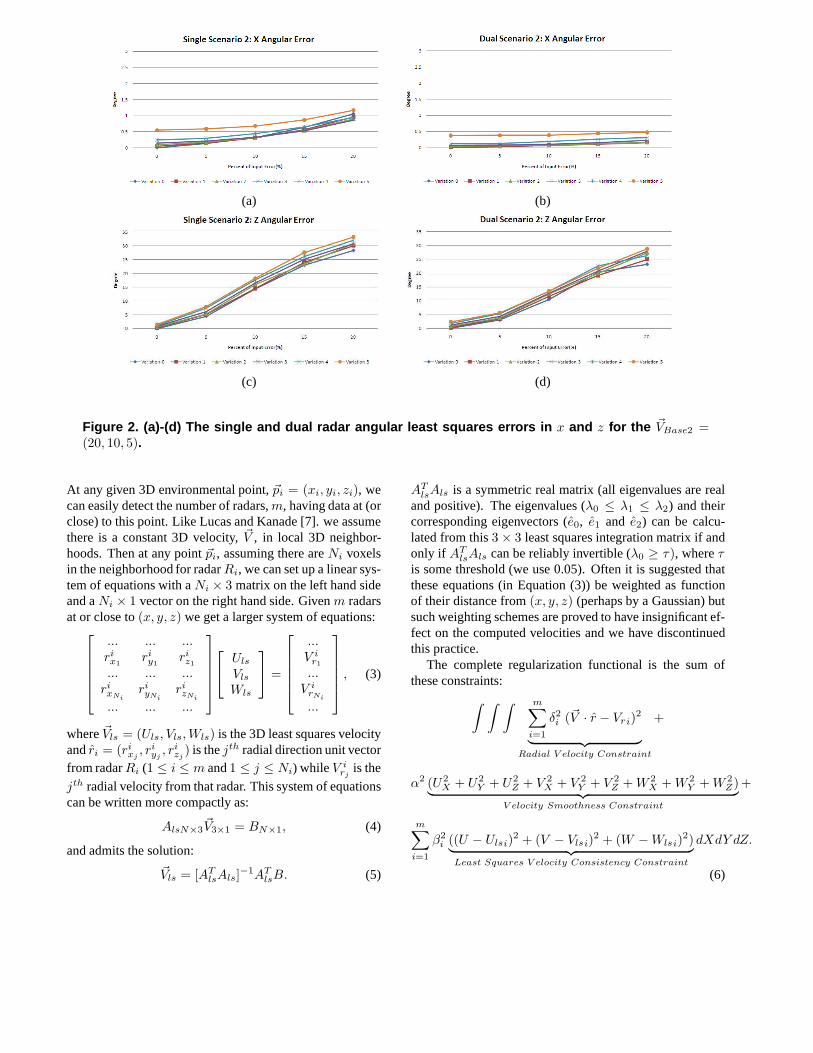
Figure 2. (a)-(d) The single and dual radar angular least squ ares errors in x and z for the ~VBase2 =(20, 10, 5).

At any given 3D environmental point,~pi = (xi, yi, zi), wecan easily detect the number of radars,m, having data at (orclose) to this point. Like Lucas and Kanade [7]. we assumethere is a constant 3D velocity,~V , in local 3D neighbor-hoods. Then at any point~pi, assuming there areNi voxelsin the neighborhood for radarRi, we can set up a linear sys-tem of equations with aNi × 3 matrix on the left hand sideand aNi × 1 vector on the right hand side. Givenm radarsat or close to(x, y, z) we get a larger system of equations:

... ... ...

rix1

riy1

riz1

... ... ...

rixNi

riyNi

rizNi

... ... ...

Uls

Vls

Wls

=

...

V ir1

...

V irNi

...

, (3)

where~Vls = (Uls, Vls, Wls) is the 3D least squares velocityandri = (ri

xj, ri

yj, ri

zj) is thejth radial direction unit vector

from radarRi (1 ≤ i ≤ m and1 ≤ j ≤ Ni) whileV irj

is the

jth radial velocity from that radar. This system of equationscan be written more compactly as:

AlsN×3~V3×1 = BN×1, (4)

and admits the solution:

~Vls = [ATlsAls]

−1ATlsB. (5)

ATlsAls is a symmetric real matrix (all eigenvalues are real

and positive). The eigenvalues (λ0 ≤ λ1 ≤ λ2) and theircorresponding eigenvectors (e0, e1 and e2) can be calcu-lated from this3 × 3 least squares integration matrix if andonly if AT

lsAls can be reliably invertible (λ0 ≥ τ), whereτ

is some threshold (we use 0.05). Often it is suggested thatthese equations (in Equation (3)) be weighted as functionof their distance from(x, y, z) (perhaps by a Gaussian) butsuch weighting schemes are proved to have insignificant ef-fect on the computed velocities and we have discontinuedthis practice.

The complete regularization functional is the sum ofthese constraints:

∫ ∫ ∫ m∑

i=1

δ2

i (~V · r − Vri)2

︸ ︷︷ ︸

Radial V elocity Constraint

+

α2 (U2

X + U2

Y + U2

Z + V 2

X + V 2

Y + V 2

Z + W 2

X + W 2

Y + W 2

Z)︸ ︷︷ ︸

V elocity Smoothness Constraint

+

m∑

i=1

β2

i ((U − Ulsi)2 + (V − Vlsi)

2 + (W − Wlsi)2)

︸ ︷︷ ︸

Least Squares V elocity Consistency Constraint

dXdY dZ.

(6)

(a) (b)

(e) (d)

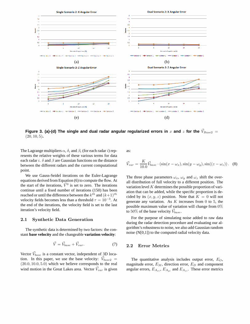
Figure 3. (a)-(d) The single and dual radar angular regulari zed errors in x and z for the ~VBase2 =(20, 10, 5).

The Lagrange multipliersα, δi andβi (for each radari) rep-resents the relative weights of these various terms for dataeach radari. δ andβ are Gaussian functions on the distancebetween the different radars and the current computationalpoint.

We use Gauss-Seidel iterations on the Euler-Lagrangeequations derived from Equation (6) to compute the flow. Atthe start of the iterations,~V 0 is set to zero. The iterationscontinue until a fixed number of iterations (150) has beenreached or until the difference between thekth and(k+1)th

velocity fields becomes less than a thresholdτ = 10−3. Atthe end of the iterations, the velocity field is set to the lastiteration’s velocity field.

2.1 Synthetic Data Generation

The synthetic data is determined by two factors: the con-stantbase velocity and the changeablevariation velocity:

~V = ~Vbase + ~Vvar . (7)

Vector ~Vbase is a constant vector, independent of 3D loca-tion. In this paper, we use the base velocity:~Vbase2 =(20.0, 10.0, 5.0) which we believe corresponds to the realwind motion in the Great Lakes area. Vector~Vvar is given

as:

~Vvar =K

10.0~Vbase · (sin(x − ωx), sin(y − ωy), sin((z − ωz)) . (8)

The three phase parametersωx, ωy andωz shift the over-all distribution of full velocity to a different position. Thevariation levelK determines the possible proportion of vari-ation that can be added, while the specific proportion is de-cided by its(x, y, z) position. Note thatK = 0 will notgenerate any variation. AsK increases from0 to 5, thepossible maximum value of variation will change from0%to 50% of the base velocity~Vbase.

For the purpose of simulating noise added to raw dataduring the radar detection procedure and evaluating our al-gorithm’s robustness to noise, we also add Gaussian randomnoise (N[0,1]) to the computed radial velocity data.

2.2 Error Metrics

The quantitative analysis includes output error,EO,magnitude error,EM , direction error,ED and componentangular errors,EAxi

, EAyiandEAzi

. These error metrics

(a) (b)

(c) (d)

Figure 4. (a) The single and (b) the dual UV Least Squares and (c) the single and (d) the dual UV Reg-ularization optical flow fields for the Detroit/Cleveland Do ppler data on August 19th, 2007 at 12:35:10.

are defined at each 3D locationi as:

EOi=

‖ ~Ve − ~Vc‖2

‖ ~Vc‖2

× 100%, (9)

EMi=

|‖ ~Vei‖2 − ‖ ~Vci

‖2|

‖ ~Vci‖2

× 100%, (10)

EDi= arccos(

~Vei· ~Vci

‖~Vei‖2‖~Vci

‖2

) ×180◦

π, (11)

EAxi= arccos(V ′

cxi· V ′

exi), (12)

EAyi= arccos(V ′

cyi· V ′

eyi), (13)

EAzi= arccos(V ′

czi· V ′

ezi), (14)

where~Veiis the retrieved velocity at locationi and ~Vci

isthe correct velocity at locationi used by the synthetic datageneration. Given estimated velocity~V e = (Vex, Vey , Vez)

and correct velocity~V c = (Vcx, Vcy, Vcz), the componentangular error calculation in Equation (12), for example, uses~V ′

ex = (Vex, 1) and~V ′

cx = (Vcx, 1). Note that we useV toindicate that~V has been normalized. The component an-gular errors provide a single numerical value that capturesboth magnitude and angular error and avoids the zero divi-sion problem inherent in relative error metrics [1].

3 Synthetic Data Results

Figures 1a and 1b and Figures 1c and 1d show the leastsquares and regularizedUV flows for the synthetic datamade using~VBase2 = (20, 10, 5), K = 5 and 20% inputerror for a single and a dual optical flow recovery. Due tospace limitations, we can not showEO, EM or ED. Sufficeit to see that there is about a 50% improvement from sin-gle to dual radar results but about 10% improvement fromleast squares to regularization We show the least squaresand regularizedx andz angular errors for single and dualradars in Figures 2 and 3. Thez velocity is more difficultto compute than thex (or y)velocity because thez directionis essentially perpendicular to thez direction (the apertureproblem). The overlapping dual data greatly aids this calcu-lation by providing more data for the calculation (increas-ing both robustness and accuracy). As well, regularizationsmoothes the flow, also increasing its accuracy.

4 Real Data Results

Figures 4a and 4b show the single and dualUV LeastSquares optical flow fields while Figures 4c and 4d showthe regularizedUV flow for single and dual radars Regu-larized optical flow fields for the Detroit/Cleveland DopplerDoppler data (on August19th, 2007 at 12:35:10). Quali-tatively, we can see that the dual flow looks better than thesingle flow in the “lens” overlapping areas of the radars andthat the regularized flow looks better than the least squaresflow for both single and dual radar data. Since the motion isessentially left to right, the “aperture” problem comes moreinto play at the upper and lower central areas of each radar.Since the lower central area of the Detroit radar is overlap-ping with the left middle of the Cleveland radar, the apertureeffects are minimized in the overlapping lens area and theflow is significantly better there.

5 Conclusions and Future Work

We have demonstrated that regularized 3D optical flowcomputed from dual radars is better than that computedfrom single regularized 3D optical flow and that regularizedflow is more accurate than the least squares flow computedfrom the same single or dual radar data [9]. Currently, weare also integrating 3D Windprofiler radar data with thesecalculations [10]. Future work includes using time-varying3D optical flow to track storms in long sequences of over-lapping Doppler and Windprofiler data.

References

[1] J. Barron, D. Fleet, and S. Beauchemin. Performance ofoptical flow techniques.Int. Journal of Computer Vision,12:43–77, 1994.

[2] J. Barron, R.E.Mercer, X. Chen, and P. Joe. 3d velocity from3d doppler radial velocity.Intl. Journal of Imaging Systemsand Technology, 15:189–198, 2005.

[3] X. Chen, J. Barron, R. Mercer, and P. Joe. 3d least squaresvelocity from 3d doppler radial velocity. InVision Interface(VI2001), pages 56–63, Ottawa, 2001.

[4] C. C. Easterbrook. Estimating horizontal wind fields bytwo-dimensional curve fitting of single doppler radar mea-surements. In16th Radar Meteorology Conference, pages214–219, 1975.

[5] B. Horn and B. Schunck. Determing optical flow.ArtificalIntelligence, 17:185–204, 1981.

[6] R. M. Lhermitte and D. Altas. Precipitation motion by pulsedoppler. InNinth Weather Radar Conference, pages 218–223, 1961.

[7] B. Lucas and T. Kanade. An iterative image-registrationtechnique with an application to stereo vision. InDARPAImage Understanding Workshop, pages 121–130, 1981.

[8] P. Waldteufel and H. Corbin. On the analysis of single-doppler radar data. Journal of Applied Meteorology,18:532–542, 1979.

[9] H. Zhang. Recovery of 3D Velocity for Storm Trackingin a Multi-Radar Framework. PhD thesis, Dept. of Com-puter Science, The University of Western Ontario, 2011. inprogress.

[10] Y. Zhang, J. Barron, and R. Mercer. 3d optical flow fromdoppler and windprofiler radar data, 2010. submitted.