1

CS 430/536Computer Graphics I

3D Modeling:Surfaces Week 8, Lecture 16

David Breen, William Regli and Maxim PeysakhovGeometric and Intelligent Computing Laboratory

Department of Computer ScienceDrexel University

http://gicl.cs.drexel.edu

2

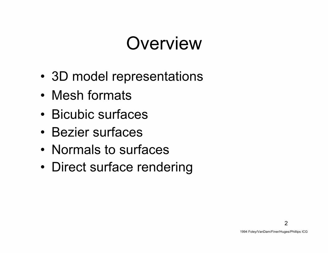
Overview

• 3D model representations• Mesh formats• Bicubic surfaces• Bezier surfaces• Normals to surfaces• Direct surface rendering

1994 Foley/VanDam/Finer/Huges/Phillips ICG

3

3D Modeling• 3D Representations

– Wireframe models– Surface Models– Solid Models– Meshes and Polygon soups– Voxel/Volume models– Decomposition-based

• Octrees, voxels

• Modeling in 3D– Constructive Solid Geometry (CSG),

Breps and feature-based

4

Representing 3D Objects

• Exact– Wireframe– Parametric

Surface– Solid Model

• CSG• BRep• Implicit Solid

Modeling

• Approximate– Facet / Mesh

• Just surfaces– Voxel

• Volume info

5

Representing 3D Objects

• Exact– Precise model of

object topology– Mathematically

represent allgeometry

• Approximate– A discretization of

the 3D object– Use simple

primitives tomodel topologyand geometry

6

Negatives whenRepresenting 3D Objects

• Exact– Complex data structures– Expensive algorithms– Wide variety of formats,

each with subtle nuances– Hard to acquire data– Translation required for

rendering

• Approximate– Lossy– Data structure sizes can

get HUGE, if you wantgood fidelity

– Easy to break (i.e. crackscan appear)

– Not good for certainapplications

• Lots of interpolation andguess work

7

Positives whenRepresenting 3D Objects

• Exact– Precision

• Simulation, modeling,etc

– Lots of modelingenvironments

– Physical properties– Many applications (tool

path generation, motion,etc.)

– Compact

• Approximate– Easy to implement– Easy to acquire

• 3D scanner, CT

– Easy to render• Direct mapping to the

graphics pipeline

– Lots of algorithms

8

Exact Representations

• Wireframe• Parametric Surface• Solid Model

– operations– CSG, BRep, implicit geometry

9

Wireframes

• Basic idea:– Represent the model

as the set of all of itsedges

• Example:A simple cube– 12 lines– 8 vertices

• How about thefaces?

Foley/VanDam, 1990/1994

11

Issues with Wireframes• Visually ambiguous• No surfaces!

– What’s inside? What’s outside?– Hidden line removal?

• What does validity entail?– Don’t we just have a bunch of wires?– Do they need to add up to something?

• How to model wireframe shapes?– Wire by wire? Not very easy!

12

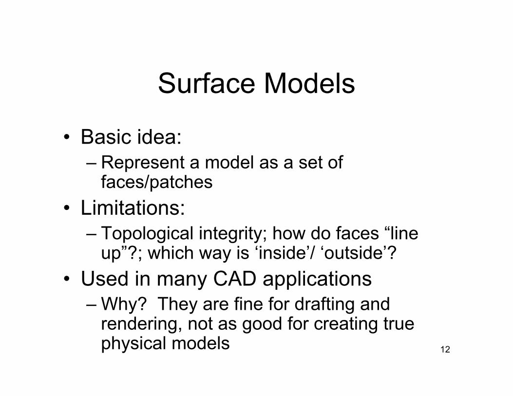
Surface Models

• Basic idea:– Represent a model as a set of

faces/patches• Limitations:

– Topological integrity; how do faces “lineup”?; which way is ‘inside’/ ‘outside’?

• Used in many CAD applications– Why? They are fine for drafting and

rendering, not as good for creating truephysical models

13

3D Mesh File Formats

Some common formats• STL

• SMF

• OpenInventor

• VRML

14

Minimal

• Vertex + Face

• No colors, normals,or texture

• Primarily used todemonstrategeometry algorithms

15

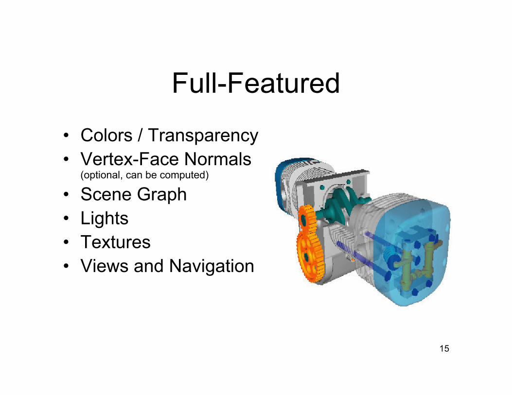
Full-Featured

• Colors / Transparency• Vertex-Face Normals

(optional, can be computed)

• Scene Graph• Lights• Textures• Views and Navigation

16

Simple Mesh Format (SMF)

• Michael Garlandhttp://graphics.cs.uiuc.edu/~garland/

• Triangle data

• Vertex indices begin at 1

17

Stereolithography (STL)

• Triangle data +Face Normal

• The de-factostandard for rapidprototyping

18

How STL Works

20

Open Inventor

• Developed by SGI• Predecessor to

VRML– Scene Graph

21

Virtual Reality ModelingLanguage (VRML)

• SGML Based

• Scene-Graph

• Full Featured

22

Issues with 3D “mesh” formats

• Easy to acquire• Easy to render• Harder to model with• Error prone

– split faces, holes, gaps, etc

23

BRep Data Structures

• Winged-Edge DataStructure (Weiler)

• Vertex– n edges

• Edge– 2 vertices– 2 faces

• Face– m edges

Pics/Math courtesy of Dave Mount @ UMD-CP

24

BRep Data Structure

• Vertex structure– X,Y,Z point– Pointers to n coincident edges

• Edge structure– 2 pointers to end-point vertices– 2 pointers to adjacent faces– Pointer to next edge– Pointer to previous edge

• Face structure– Pointers to m edges

25

Biparametric Surfaces

• Biparametric surfaces– A generalization of parametric curves– 2 parameters: s, t (or u, v)– Two parametric functions

26

Bicubic Surfaces

• Recall the 2D curve:– G: Geometry Matrix– M: Basis Matrix– S: Polynomial Terms [s3 s2 s 1]

• For 3D, we allow the points in G to vary in 3Dalong t as well:

27

Observations AboutBicubic Surfaces

• For a fixed t1,is a curve

• Graduallyincrementing t1 to t2,we get a new curve

• The combination ofthese curves is asurface

• are 3D curves

28

Bicubic Surfaces

• Each is , where

• Transposing , we get

29

Bicubic Surfaces

• Substituting into ,we get Q(s, t)

• The g11, etc. are the control points for theBicubic surface patch:

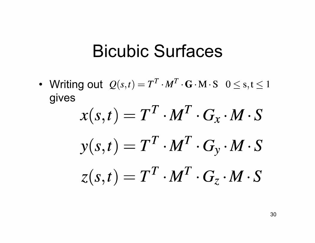
30

Bicubic Surfaces

• Writing outgives

32

Bézier Surfaces

• Bézier Surfaces(similar definition)

33

Faceting

34

Plotting Isolines

35

Faceting

36

Bézier Surfaces

• C0 and G0 continuitycan be achievedbetween twopatches by settingthe 4 boundarycontrol points to beequal

• G1 continuityachieved whencross-wise CPs areco-linear

37

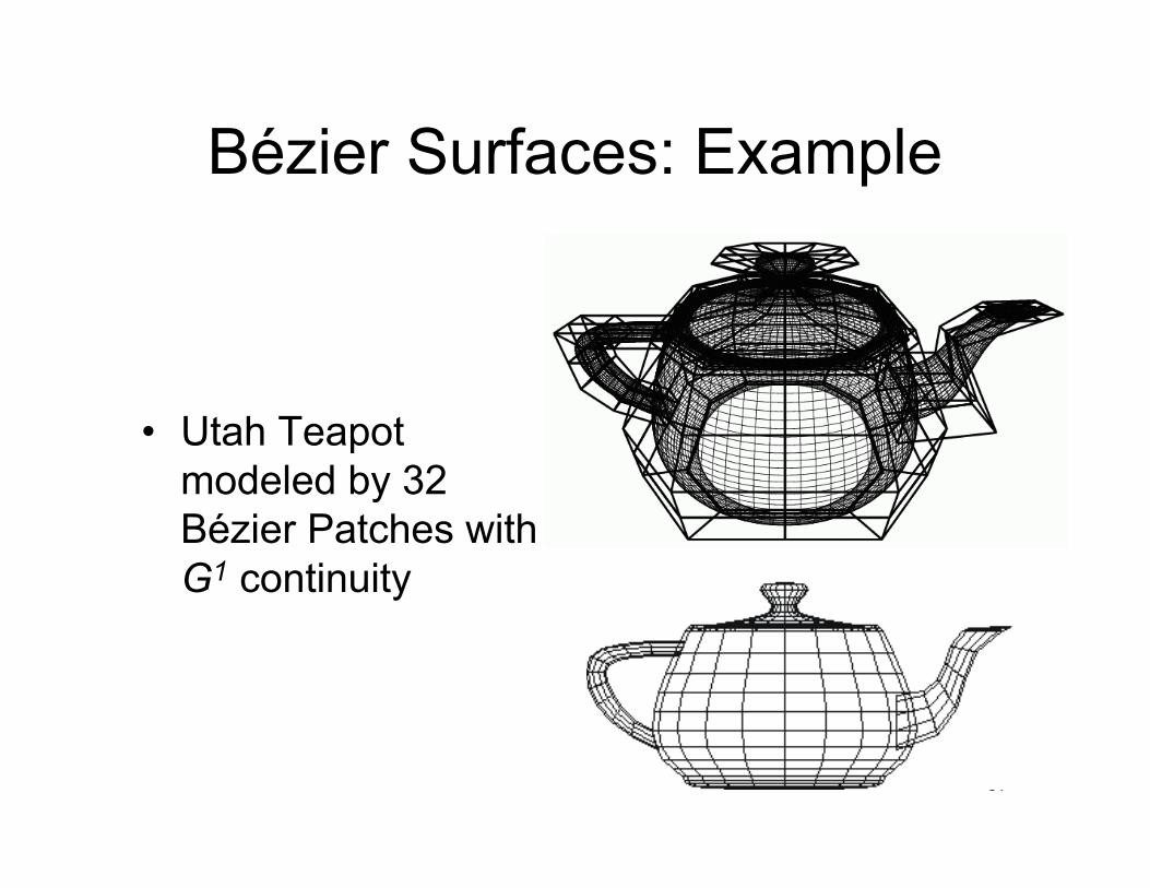
Bézier Surfaces: Example

• Utah Teapotmodeled by 32Bézier Patches withG1 continuity

38

Bezier Surface: Example

• Increased facetresolution

• Rendered

39

B-spline Surfaces

• Representation for B-spline patches• C2 continuity across boundaries is automatic

with B-splines

40

Normals to Surfaces

• Normals used for– Shading– Interference detection

in robotics– Calculating offsets for

numerically controlledmachining

41

Computing theNormals to Surfaces

• For a bicubic surface,first, compute the s tangent vector

42

Computing theNormals to Surfaces

• Next, compute the t tangent vector:

t

43

Computing theNormals to Surfaces

• Since s and t are tangent to the surface,their cross product is the normal vector to thesurface!

• xs - x component of s tangent• ys - y component of s tangent• zs - z component of s tangent

45

Drawing Parametric Surfaces

• Usually done “patch by patch”• Two choices

– Draw/render directly from the parametricdescription

– Approximate the surface with a polygonmesh, then draw/render the mesh

46

Direct Rendering

• Use a scan-line algorithm– Evaluate pixel by pixel– Problem: How to go from (x,y) “screen

space” to point on the 3D patch• Easy for a planar polygon where we know

max/min y, equations for edges, screen depth• Not as easy for parametric surfaces

47

Issues for Direct Rendering

• Max/Min y coords may not lie on boundaries• Silhouette edges result from patch bulges

– Need to track both silhouettes and boundaries• What if they intersect?• Note: patch edges need not be monotonic in x or y

• Idea: Scan convert patch plane-by-plane, using scanplanes instead of scan lines

48

Direct Scan Conversion ofPatches

– Patch: x=X(u,v), y=Y(u,v), z=Z(u,v)

• Basic idea– Find intersection of

patch with XZ plane• Producing a planar curve

– Draw the curve• De Boor, D’Casteljeau

– Note: if doing rendering,one can compute pixel-by-pixel color valuesthis way

50

Patch to Polygon Conversion

Two methods:• Object Space Conversion

– Techniques• Uniform subdivision• Non-uniform subdivision

– Resolution: depends on object space• Image Space Conversion

– Resolution: depends on pixels and screen

51

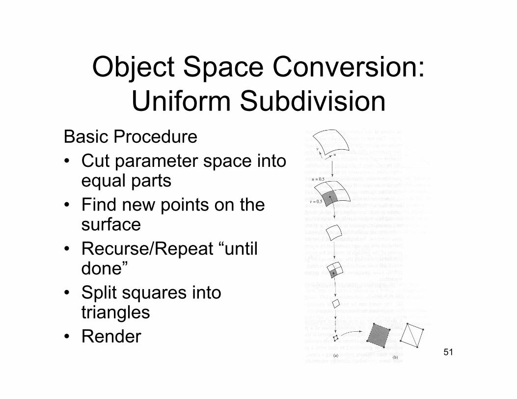
Object Space Conversion:Uniform Subdivision

Basic Procedure• Cut parameter space into

equal parts• Find new points on the

surface• Recurse/Repeat “until

done”• Split squares into

triangles• Render

52

Object Space Conversion:Non-Uniform Subdivision

• Basic idea– More facets in areas of high curvature– Use change in normals to surface to

assess curvature• More derivatives

– Break patch into sub-patches based oncurvature changes

53

Image Space Conversion

• Idea: control subdivision based onscreen criteria– Minimum pixel area

• Stop when patch is basically one pixel– Screen flatness

• Stop when patch converges to a polygon– Screen flatness of silhouette edges

• Stop when edge is straight or size of pixel

54

How do I know if I’ve found asilhouette edge?

• If the viewing ray is tangent to thesurface at the point it hits the surface!N • L = 0– Where N is the normal at the point where L,

the line of sight, hits the surface