Confocal, Multiphoton, and Nonlinear Imaging, Tony Wilson, Editor, 67 Proceedings of SPIE-OSA Biomedical Optics, SPIE Vol. 5139 (2003) Copyright 2003 Society of Photo-Optical Instrumentation Engineers. This paper was (will be) published SPIE Vol. 5139 and is made available as an electronic reprint with permission of SPIE. One print or electronic copy may be made for personal use only. Systematic or multiple reproduction, distribution to multiple locations via electronic or other means, duplication of any material in this paper for a fee or for commercial purposes, or modification of the content of the paper are prohibited.

3D Imaging and Quantification of Complex Vascular Networks

Paul R. Barber*a, Simon M. Ameer-Bega, Borivoj Vojnovica, Richard J. Hodgkissa, Gillian M. Tozerb, John Wilsonb, Vivien E. Priseb

aAdvanced Technology Development Group; bTumour Microcirculation Group, Gray Cancer Institute

ABSTRACT The understanding of tumour angiogenesis and response to vascular-targeted drugs are of increasing interest in cancer research. We present 3D images of the in vivo tumour vasculature captured utilising multi-photon microscopy together with the results of manual and semi-automated delineation of the vascular network using novel in-house-developed software and algorithms. The software presented is aimed at aiding in these investigations and other problems where linear or dendritic structures are to be delineated from 3D data sets. A new algorithm, CHARM, based on a compact Hough transform and the formation of a radial map, has been used to automatically locate vessel centres and measure diameters. The robustness of this algorithm to image smoothing and noise has been investigated. Statistical information characterising the network in terms of vascular parameters as well as more complex analyses, such as fractal dimension, are now possible and examples are presented.

Keywords: Multiphoton, In-Vivo, Image Processing, Network, Fractal Dimension, hypoxia, angiogenesis, Hough transform, quantification.

1. INTRODUCTION In the field of cancer research there is currently a high level of interest in understanding tumour angiogenesis and the response to vascular-targeted drugs. Hypoxia, which can develop in tumour regions that are sparsely vascularised or have low blood flow, affects tumour response to treatment and acts as a stimulus for the production of angiogenic factors1. In understanding the action of vascular-targeted drugs, such as combretastatin A4 phosphate which has been shown to have an anti-cancer effect2, there is a need to measure, quantify and model vascular structures. This can be achieved through studies at the biochemical, cellular and complete tissue levels.

Recent technological developments in two-photon fluorescence microscopy have enabled the imaging, in 3D, of both normal and cancerous tissue within the dorsal skin flap of a rodent with the so-called ‘window-chamber’2. We have captured in vivo three-dimensional data sets via a window chamber arrangement with a multi-photon microscope3 in a manner similar to that employed by Jain and co-workers4. In short, imaging contrast was achieved by i.v. injection of cascade blue or FITC labelled high molecular weight (70 kD) dextran which acts as a fluorescent marker of blood plasma under two-photon excitation. A particular problem is that the physical arrangement of the window chamber in the microscope limits the objectives lenses that can be used to those of low magnification and numerical aperture. The result is a highly non-spherically symmetric, optical point spread function (PSF). We present the results of imaging and a software application that was written to analyse such data sets by allowing the manual and semi-automated tracking and delineation of the vascular network, including the measurement of vessel diameter. The aim was to facilitate investigations of the vascular structure of complete and living tissue and the methods may also be applicable to other problems where similar structures are to be delineated from 3D data sets.

* barber@gci.ac.uk; phone: +44 (0) 1923 828611; fax: +44 (0) 1923 835210; http://www.gci.ac.uk; Advanced Technology Development Group, Gray Cancer Institute, Mount Vernon Hospital, Northwood, Middlesex, HA6 2JR, UK;

68 Proc. of SPIE Vol. 5139

There have previously been several approaches to the delineation of tree-like structures but our images generally have highly complex and incomplete trees that may be disjointed, against a high-noise background that are a challenge to segment by eye. The validation of any automated approach does require a gold standard, which at the present time is the manually segmented image. For this reason we thought it appropriate to form an application with a set of both manual and semi-automatic tracing tools. Most effort by others has been producing algorithms for extracting information from 2D images (for example: deformable models5; fuzzy clustering of profiles6) but there has been progress in the 3D arena7-10. These current studies are aimed at furthering this understanding by 3D imaging of the in vivo vascular structure, interactive delineation of the vascular network and by the collection of statistical data that can characterise different types of normal and tumour tissue. The delineation of the vascular network enables much more informative studies of the tissue structure to be undertaken. The understanding of tumour hypoxia can be extended through the formation of the 3D Euclidean distance map which highlights and quantifies areas of the tissue that are not well vascularised and therefore are likely to experience hypoxia. The study of the structures fractal dimension is also of interest as is the vessel tortuosity. The results of such statistical analysis of fractal dimension, vessel tortuosity and the formation of a Euclidean distance map are given.

2. METHODOLOGY 2.1 MULTI-PHOTON IMAGING

Microscopy was performed with a multiphoton microscope system, based on a modified Bio-Rad MRC 1024MP workstation, comprising a solid-state-pumped (10 W Millennia X, Nd:YVO4, Spectra-Physics), self-mode-locked Ti:Sapphire (Tsunami, Spectra-Physics) laser system, afocal scan-head, confocal detectors and an inverted microscope (Nikon TE200). Enhanced detection of the scattered component of the emitted (fluorescence) photons is afforded by the use of three, in-house developed, non-descanned detectors, situated in the re-projected stationary plane (re-imaged objective back aperture). Due to geometrical constraints of the animal models, long working distance objectives must be used and, unless otherwise stated, a 10x Nikon Plan Fluor objective was used (16 mm WD, 0.3 NA) for in vivo imaging.

Measurement of the optical PSF within the sample was estimated with the use of 3 µm fluorescent beads injected via the tail vein of the rodent. A proportion of the beads became trapped within the vascular tree. The observed bead profiles did not differ significantly from those observed in the ideal conditions of slide-mounted beads or the theoretical prediction based on the use of this objective lens. The PSF was approximately 1 µm FWHM in the transverse directions X and Y, and approximately 10 µm in the axial direction, Z.

2.2 DORSAL SKINFOLD WINDOW CHAMBERS

HT29 human xenograft and P22 rat carcinosarcoma tumours were grown in transparent window chambers, surgically implanted into the dorsal skin flap of mice (HT29) and rats (P22)2. For in vivo imaging, a specially adapted microscope stage allows mounting and positioning of the window chamber above the microscope objective. Prior to imaging the rats were anaesthetised with Hypnorm and midazolam11; the mice were conscious throughout and placed in a Perspex restraining jig. Body temperature was regulated using a thermostatically-controlled heating pad with rectal temperature sensing. For imaging of the blood vessel architecture, a 70 kD anionic dextran conjugated with either Cascade BlueTM or FITC (Molecular Probes) was injected intravenously as a blood pool contrast agent.

2.3 SOFTWARE METHODS

The software was developed under the LabWindows/CVI (National Instruments Corporation) environment in the C programming language and tested on both real and synthetic 3D data sets. The 32-bit application runs on a PC under the Windows NT4, 2000 or XP operating systems. At GCI the software is run under Windows2000 (Microsoft, USA) on a PC (Dell, UK) with dual Xeon processors (1.7 GHz) (Intel, USA), 1 Gb of RAM and an Nvidia QuadroPro graphics card (Nvidia, USA). This computer also runs more-computationally intensive visualization software and is more than sufficient to run the tracing software, which has been run comfortably on a single-processor 500 MHz PIII (Intel, USA)

Proc. of SPIE Vol. 5139 69

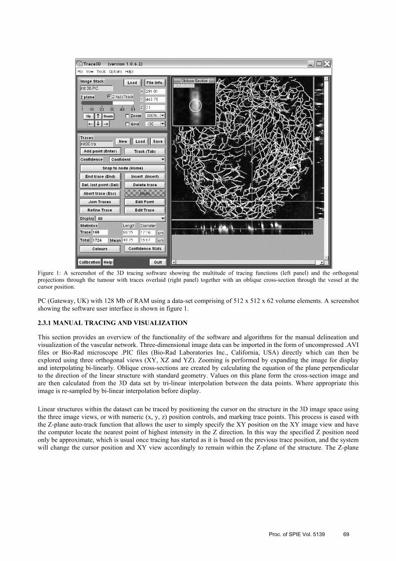
Figure 1: A screenshot of the 3D tracing software showing the multitude of tracing functions (left panel) and the orthogonal projections through the tumour with traces overlaid (right panel) together with an oblique cross-section through the vessel at the cursor position.

PC (Gateway, UK) with 128 Mb of RAM using a data-set comprising of 512 x 512 x 62 volume elements. A screenshot showing the software user interface is shown in figure 1.

2.3.1 MANUAL TRACING AND VISUALIZATION

This section provides an overview of the functionality of the software and algorithms for the manual delineation and visualization of the vascular network. Three-dimensional image data can be imported in the form of uncompressed .AVI files or Bio-Rad microscope .PIC files (Bio-Rad Laboratories Inc., California, USA) directly which can then be explored using three orthogonal views (XY, XZ and YZ). Zooming is performed by expanding the image for display and interpolating bi-linearly. Oblique cross-sections are created by calculating the equation of the plane perpendicular to the direction of the linear structure with standard geometry. Values on this plane form the cross-section image and are then calculated from the 3D data set by tri-linear interpolation between the data points. Where appropriate this image is re-sampled by bi-linear interpolation before display.

Linear structures within the dataset can be traced by positioning the cursor on the structure in the 3D image space using the three image views, or with numeric (x, y, z) position controls, and marking trace points. This process is eased with the Z-plane auto-track function that allows the user to simply specify the XY position on the XY image view and have the computer locate the nearest point of highest intensity in the Z direction. In this way the specified Z position need only be approximate, which is usual once tracing has started as it is based on the previous trace position, and the system will change the cursor position and XY view accordingly to remain within the Z-plane of the structure. The Z-plane

70 Proc. of SPIE Vol. 5139

auto-track function eases the manual finding of the structure to be traced, in 3D, by automatically locating the nearest bright structure, at the current XY position, by moving the cursor position in the Z direction. Therefore, as the user moves the cursor position in the XY plane, step-wise, along a tubular structure to be traced, the cursor Z position is automatically updated to maintain the cursor position at the centre of the structure. Z-plane auto-tracking is performed by forming a 1D array of values, which are taken from each Z-plane at the cursor position (x, y). A ‘hill-climbing’ algorithm is applied to this array to find the nearest peak in intensity. A valley finding algorithm can be used if the structure is dark compared to the background. To reduce the effect of noise, the value from each Z-plane used is an average of a square of pixels, typically a 3 x 3 area. The array formed is further filtered (filtering in the Z-direction) by a 3-point moving average.

When using difficult to track, noisy or unclear data the user can associate one of three confidence levels with each point traced. These have been named ‘Confident’, ‘Tentative’ and ‘Guesswork’ and are displayed in different colours. Using these labels it is easier to quantify the reliability of the data and derive appropriate statistics. Basic statistics about the tracings are shown on the front panel. Measurement of the trace lengths and mean diameters are made and reported for all traces and the current or selected trace. In addition, several general trace-point deletion, selection and insertion functions have been incorporated for trace editing.

Traces are stored in memory in the form of a list of 3D floating-point coordinates, in pixel dimensions. Each point also has a floating-point radius, in pixel dimensions, and a confidence flag associated with it. The calibration factors, for conversion to real coordinates, can be set by the user. The traces can be saved in a text file as a list of coordinate points, which can be re-loaded into memory. The traces can also be exported in the form of a virtual reality world file (*.WRL) using the Virtual Reality Modelling Language (VRML) version 2.0, also known as VRML97*. The traces can be formed by single pixel lines using the ‘IndexedLineSet’ geometry or as solid cylinders (‘Cylinder’ geometry) representing the measured structure diameter. Such files can be imported into 3D surface rendering packages for viewing and for overlaying onto a 3D volume rendering of the original data. In this way the traces can be verified by eye in great detail with the use of 3D zooming, panning and rotation tools.

2.3.2 SEMI-AUTOMATED TRACING

This section details the algorithms that perform the semi-automated functions.

Diameter measurement and centre location of the structure is performed by an algorithm that has been named the Compact Hough transform And Radial Map (CHARM) from the oblique cross-section through the structure. The compact Hough transform was recently used successfully in an automated colony counter12 and has been reapplied here to find the approximate centre position of circular objects (the shape of most vessels in cross-section). The CHARM algorithm works on an oblique cross-section image centred on an approximate vessel centre. It applies two perpendicular Sobel edge-detection filters13. A compact Hough transform is applied to the resulting edge maps and gives the largest response to bright circular objects. The pixel with the greatest response is taken as a point within the structure to be measured. This implementation differs from that previously described only by the fact that floating-point values for the centre location are maintained throughout for improved accuracy.

Radial searching is performed from this centre point to find likely object boundary points14, 15 based on the response of the Sobel filters. The searching range is based on an approximate seed radius and is typically 0.75 to 1.5 times this value. The edges, identified by a significant Sobel response of the correct orientation, form a radial map that describes the shape. Some filtering of this map is required to eliminate distraction from unwanted structure, and the effect of a non-spherical imaging point spread function (PSF). The 32-point maps were spatially filtered with a 3-point median filter. The centre of mass16 of the 2D shape described by the radial map was taken as an accurate measurement of the vessel centre. The diameter measurement was calculated statistically from the median of the 32 radius measurements.

* ISO/IEC 14772-1:1997.

Proc. of SPIE Vol. 5139 71

The general direction of the vessel or linear structure is known from adjacent trace points and this can be used to calculate an oblique cross-section through the structure orthogonal to its direction in 3D space. The oblique cross-section calculated is used to measure the diameter of the structure at this point using the CHARM algorithm. This also determines a centre of mass for the structure that is used to update the trace point position. When manual tracing the oblique cross-section is displayed as an image with the measured centre position and diameter overlaid for the user to verify.

The automatic measurement of structure centre-position and diameter allows the software to automatically track the remainder of a structure given a start of two manually traced points by proceeding along the structure in a stepwise manner, measuring the diameter and refining the trace position at each point. The size of the steps can be specified but steps equal to the current radius are usually successful. The steps, and indeed, the separation of the initial manual points, should not be much greater than the vessel diameter to ensure that the structure is nominally straight between points. The estimate for the next centre position is based on the current direction of the linear structure based on the previous two points. It is assumed that this direction is continued and we move in that direction by one step. A further enhancement is to take account of the current structure curvature based on the last three points and assume that this continues to the new position.

At the new position, the diameter measurement algorithm is used to measure the structure diameter and to update the centre position. It can sometimes be assumed that the measurement of centre position is much closer to the real position than the estimate, if the data is very clean. More robust tracking, through noisy data, is often achieved by applying a Kalman filter17 to the update of position and diameter measurement. In this case the estimate of the next centre position is formed from a linear combination of the predicted position based on past data and of the measured position based on new data. Ideally, each contribution is inversely weighted by its error but, since these error values are difficult to measure, they are estimated and suitable weights can be arrived at empirically. The filter has been made adaptive by adjusting the weight applied to the new measurement according to the standard deviation of the 32 radial measurements. In this way a higher preference can be given to the new measurement in areas of the data set which are particularly clean and where reliable measurements can be made.

2.3.3 TEST METHODS

Testing of the measurement accuracy of the CHARM algorithm was performed on artificial test images. These were created from a binary-image approximation to a circle with a diameter of 10 pixels, which was smoothed and had noise added (see Figure 2). Resulting images were stacked together to form a 3D image, 20 images deep, which can be traced to produce 18 measurements of centre location and diameter (excluding 2 measurements at the image extremes). Smoothing was performed by 2D convolution with a floating-point Gaussian kernel with standard deviation (σ) ranging from 0.0 to 5.0 pixels. The kernel size was always four times the standard deviation. Random Gaussian noise with standard deviation (σ) ranging from 0.0 to 50.0 grey levels was added on a pixel-by-pixel basis, after smoothing. When forming 3D image stacks from noisy data, noise was added to each image slice independently. The range of smoothing and degrees of noise were chosen to span those typically observed in real data. The 18 measurements of location and diameter were averaged to ascertain the performance of the algorithm.

The effect of a non-symmetrical imaging PSF on the performance of the algorithm was also demonstrated by applying a 1D Gaussian filter to apply additional smoothing in one direction (Figure 6, f - j). It is also interesting to demonstrate the ability of the semi-automatic tracing in the presence of a high degree of image smoothing and noise. 3D images of two, closely

Figure 2: Test images were made by adding Gaussian noise and smoothing to a binary circle.

72 Proc. of SPIE Vol. 5139

spaced, tubular structures were created, based on the binary circle of 10-pixel diameter. In these test images, one tubular structure lies on an arc of radius 50 pixels and is separated at the closest point by one pixel from the second structure which lies on a straight line (Figure 7).

3. RESULTS A screenshot of the software in use can be seen in figure 1, the XY, XZ and YZ cross-section images can be seen on the right hand panel overlaid by the lines of tracings already made. It can be seen how the oblique cross-section image is presented to the user with the vessel diameter measurement overlaid in white.

To investigate the effects of image smoothing and noise on the performance of the algorithm artificial test images were used to determine an error in the diameter measurement and also in the measured centre location. The results of these tests can be seen in figure 3 and as could be expected the addition of smoothing and noise has a detrimental effect on the measured diameter and centre location. Below a reasonable extreme smoothing of 5.0 pixels in width, the error in diameter measurement was never above 13% (1.3 pixels in 10.0) and in centre location it was never above 0.7 pixels. It appeared that smoothing is more detrimental than the addition of noise. To demonstrate how different seed values of approximate vessel centre and radius change the results, these were varied in the presence of different degrees of smoothing. The results are presented in figure 4 and it can be seen that the measured centre location is not affected by varying the seed centre location. In practice, however, the measurement is made from an oblique cross-section image that is of finite size, the vessel must be wholly contained within it for the algorithm to succeed. The seed radius must be close enough to the true value for it to be found within the limits of the radial search (typically 0.75 to 1.5 times the seed value) and outside these limits the algorithm fails. Within these limits the error in diameter measurement was always below 9% (0.9 pixels in 10.0) and the centre was located to within 0.5 pixels. In practice automatic diameter measurement can be seeded by previous measurements at other points on the same vessel whilst tracking or, where no such measurements exist, on an initial manual measurement.

The primary aim of this work is to facilitate the tracing of images produced by our multi-photon microscope, which, for reasons explained above, has a non-symmetric PSF. Figure 5 visually demonstrates the performance of the algorithm in the presence of symmetrical and non-symmetrical Gaussian smoothing. The diameters measured for symmetrical smoothing of σ = 0.0, 2.0, 4.0 6.0 and 8.0 pixels (Figure 6, a, b, c, d and e) were 9.92, 9.92, 9.64, 9.96 and 10.76, respectively (actual diameter 10.0). A non-symmetrical PSF was simulated by the addition of 1D smoothing. Symmetrical smoothing of width 1.0 was augmented by directional smoothing of σ = 2.0, 4.0, 6.0, 8.0 and 10.0 pixels (Figure 6, f, g, h, i and j). The measured diameters were 9.93, 9.98, 10.05, 10.14 and 10.51 respectively.

Figure 3: The addition of image smoothing and noise leads to larger errors in the automatic measurement of diameter (a) and vessel centre location (b).

Proc. of SPIE Vol. 5139 73

Figure 4: The error in the measurements of diameter (a, c) and centre location (b, d) as a function of image smoothing and an offset in the centre pixel (a, b) or varying the radius (c, d) used to seed the CHARM algorithm.

Three examples of tracing closely spaced tubular structures are presented in figure 6. Sub-images a, b and c show cross sections through the centre of test 3D image stacks that where manually created to simulate two separate vessels passing close to each other. No smoothing or noise was added to the image shown in a, whereas b and c were smoothed with σ of 5.0 and 6.0 pixels respectively and both had noise of σ=50.0 pixels added. Sub-images d, e and f show qualitatively the results of automatic tracing, seeded by two points (represented by the arrows), as surface rendered objects. Figure 6e shows the successful segmentation of the two structures whereas figure 6f shows how the algorithm may fail by merging the two structures. In all surface rendered traces shown, a cylinder of constant diameter that reflects the mean measured diameter, represents each trace. Each trace has been capped with a sphere, of the same diameter, on each end to improve the appearance.

74 Proc. of SPIE Vol. 5139

Figure 5: Results of diameter measurement of a circle with true diameter of 10.0 pixels (a), with symmetrical Gaussian smoothing of σ = 2.0, 4.0 6.0 and 8.0 pixels (b, c, d and e), and with 1D smoothing of σ = 2.0, 4.0, 6.0, 8.0 and 10.0 pixels (in addition to symmetrical smoothing of σ = 1.0) (f, g, h, i and j), as indicated in the right margin.

To demonstrate typical results of tracing in-vivo vascular structure using the described techniques, two tumours, within dorsal skin-flap window chambers, where imaged via multi-photon microscopy. The images were traced using the manual and semi-automatic techniques of the described software by competent personnel and the results of tracing were used to produce some statistics about the vascular networks. An HT29 human xenograft and a P22 rat carcinosarcoma where analyzed. Figure 7 presents the results of vessel tracing together with volume renderings of the original data for comparison. Once the vascular network has been traced and a vector description has been obtained it is then possible to calculate statistical data about the network as a whole. We have written additional software programs to produce such statistics based on vessel length (distance between branching points, L, and shortest path between branching points, SP), diameter (D), surface area, volume (V) as well as measurements of vascular density such as filled volume (Vf, %) and number density (µm-3) by measuring the tumour bounding volume. Also of interest are measurements of vessel tortuosity (T, %) and we have implemented a measurement based on that of Norrby18:

1001 ×

−=

LSPT 1

The study of the structures fractal dimension is also of interest as it has been shown that it can distinguish between local (percolation-like), diffusion-limited, and compact growth processes and that the tumour vascular is similar in nature to a percolation cluster19. We have used published c-language source code20 to make measurements of fractal dimension. The Fractal dimension of the network has been estimated by calculating the capacity dimension by the so-called “box counting” method21. The fractal dimensions of the two test networks where calculated in 3D and when projected onto a single Z plane (2D) and the results are presented in table 1.

Embedding Dimension

HT29 P22 Diffusion-limited Percolation Compact growth

2 1.69 1.86 1.6722 1.8919 2.0019 3 1.76 2.06 2.5022 2.5223 3.0019

Table 1: Fractal dimensions for the two example tumours with known values for comparison.

Proc. of SPIE Vol. 5139 75

Figure 6: Tracing two tubular structures that are separated by one pixel at the closest point. Shown are cross-sections through the centre of the volume data with no noise or smoothing (a) and with Gaussian noise added (σ = 50.0) and smoothing of σ = 5.0 (b) and 6.0 (c). The results of automatic tracing are represented in d to f, the arrows indicating the given starting points for tracing.

The results concur with the assertion that the vasculature of tumours does not form space-filling (compact) structures as normal capillary networks and indeed the P22 tumour, which is well vascularised, does exhibit a fractal dimension representative of a percolation structure when embedded in 2D. When the full 3D data is taken into account the results of fractal dimension are lower than expected. This is probably due to the physical arrangement of the window chamber model in that the tumour is some-what confined in 2 dimensions.

The understanding of tumour hypoxia can be extended through the formation of the 3D Euclidean distance map which highlights and quantifies areas of the tissue that are not well vascularised and therefore are likely to experience hypoxia. Calculating the distance map by standard 3-dimensional geometry reveals that the mean interstitial distances to the nearest vessel for the example HT29 and P22 tumours are 131 and 39 µm respectively. The HT29 is indeed a hypoxic tumour24 and the P22 is well vascularised25.

A summary of the statistical data collected for the two example tumours is shown in figure 8. Analysis of the statistics for a number of tumours of different types will be the subject of further studies.

4. CONCLUSIONS In conclusion, we have presented a software application that enables the user to semi-automatically delineate and trace linear structures in 3D. The software was written to collect data on vascular networks in vivo within the animal window-chamber model. This has been achieved by employing two-photon microscopy and the software presented. However, the software package is equally applicable to similar problems involving 3D volumetric data sets from other sources, such as the tracing of neurons or bone structures. Additional data analysis packages have been written to quantify the structure in terms of statistical measures. For example, the mean distance between vessels branches, the mean diameter

76 Proc. of SPIE Vol. 5139

and tortuosity are all of interest when quantifying the differences in vascular structure between normal and tumour tissue. Other more complex analysis such as calculating the fractal dimension and the distance map, have also been made.

Figure 7: Example HT29 (a, b and c) and P22 tumours (d, e and f) traced using the presented software. Sub-images a and d show all traces projected onto the 2D XY plane, b and e show the original volume rendered data, c and f show the surface rendered traced vascular networks.

The export of the structure in virtual reality (VRML) format allows the easy validation of the traced structures by eye using commercially available surface rendering packages in the fully 3D arena. Through the use of the Hough transform the algorithm is capable of detecting multiple vessel centres, if they exist, within the oblique cross-section. In this way it should be possible to detect and locate branching points, in 3D, by the change to a bimodal distribution, in a way similar to the 2D algorithm of Tolias and Panas 6. In the future, this work will also aid the production of realistic mathematical models of tumour angiogenesis and re-modelling.

Proc. of SPIE Vol. 5139 77

0

20

40

60

80

100

120

140

L

µm

0

5

10

15

20

25

30

D

µm

0

5

10

15

20

25

30

35

T

%

0

2

4

6

8

10

12

Vf

%

0

0.5

1

1.5

2

2.5

Df0

20

40

60

80

100

120

140

Ln

µm

Figure 8: Statistics collected for 2 example tumours: HT29 and P22. Statistics shown are mean vessel length (L), mean vessel diameter (D), mean vessel tortuosity (T), volume % filled by the vascular structure (Vf), fractal (capacity) dimension (Df) and mean interstitial distance to the nearest vessel (Ln). Error bars, where shown, indicate the spread of measurements in the network.

ACKNOWLEDGEMENTS The authors gratefully acknowledge the support of Cancer Research UK under programme grant C133/A1812 – SP2195-01/02.

REFERENCES 1. Vaupel, P., Kelleher, D. K. and Hockel, M. "Oxygen status of malignant tumors: pathogenesis of hypoxia and

significance for tumor therapy." Seminars in Oncology 28, 29-35 (2001). 2. Tozer, G. M., et al. "Mechanisms Associated with Tumor Vascular Shut-Down Induced by Combretastatin A-4

Phosphate: Intravital Microscopy and Measurement of Vascular Permeability." Cancer Research 61, 6413-6422 (2001).

3. Ameer-Beg, S. M., et al. "Application Of Multiphoton steady state and lifetime imaging to mapping of tumour vascular architecture in vivo." Proc. SPIE 4620, 85-95 (2002).

4. Brown, E. B., et al. "In vivo measurement of gene expression, angiogenesis and physiological function in tumors using multiphoton laser scanning microscopy." Nature Medicine 7, 864-8 (2001).

5. Bulpitt, A. J. and Berry, E. in Medical Image Understanding and Analysis 98 (eds. Berry, E., Hogg, D. C., Mardia, K. V. and Smith, M. A.) 25-28 (University Print Services, Leeds, UK, 1998).

6. Tolias, Y. A. and Panas, S. M. "A fuzzy vessel tracking algorithm for retinal images based on fuzzy clustering." IEEE Trans. Medical Imaging 17, 263-273 (1998).

7. Serra, L., Hern, N., Choon, C. B. and Poston, T. in Proceedings of the 1997 Symposium on Interactive 3D Graphics (eds. Cohen, M. and Zeltzer, D.) 131-137 (ACM Press, NY, USA, Providence, Rhode Island, USA, 1997).

8. Dima, A., Scholz, M. and Obermayer, K. "Automatic three-dimensional graph construction. of nerve cells from confocal microscopy." J-Electron-Imaging 12, 134-150 (2003).

9. Maddah, M., Afzali-Kusha, A. and Soltanian-Zadeh, H. "Efficient center-line extraction for quantification of vessels in confocal microscopy images." Medical Physics 30, 204-211 (2003).

10. Yi, D. and Hayward, V. "Skeletonization of Volumetric Angiograms for Display." Computer Methods in Biomechanics & Biomedical Engineering 5, 329 - 341 (2002).

11. Tozer, G. M. and Shaffi, K. M. "Modification of tumour blood flow using the hypertensive agent, angiotensin II." Br. J. Cancer 67, 981-988 (1993).

12. Barber, P. R., et al. "Automated Counting of Mammalian Cell Colonies." Physics in Medicine and Biology 46, 63-76 (2001).

13. Sobel, I. in Machine Vision for Three-Dimensional Scenes (ed. Freeman, H.) 376-379 (Academic Press, 1990).

HT29

P22

78 Proc. of SPIE Vol. 5139

14. Mouroutis, T., Roberts, S. J. and Bharath, A. A. "Robust cell nuclei segmentation using statistical modelling." Bioimaging 6, 79-91 (1998).

15. Barber, P. R., et al. in Medical Image Understanding and Analysis, MIUA2000 (eds. Arridge, S. and Todd-Pokropek, A.) 41-44 (Communications in Print Plc, UCL, London, UK, 2000).

16. Russ, J. C. The Image Processing Handbook (CRC Press, 1999). 17. Maybeck, P. S. Stochastic models, estimation, and control (Academic Press Inc., New York, 1979). 18. Norrby, K. "Microvascular density in terms of number and length of microvessel segments per unit tissue

volume in mammalian angiogenesis." Microvascular Research 55, 43-53 (1998). 19. Gazit, Y., et al. "Fractal Characteristics of Tumor Vascular Architecture During Tumor Growth and

Regression." Microcirculation 4, 395-402 (1997). 20. Sarraille, J. J. and Myers, L. S. "Fd3 - a Program for Measuring Fractal Dimension." Educational and

Psychological Measurement 54, 94-97 (1994). 21. Liebovitch, L. S. and Toth, T. "A fast algorithm to determine fractal dimensions by box counting." Physics

Letters A 141, 386-390 (1989). 22. Meakin, P. "Diffusion-controlled cluster formation in 2—6-dimensional space." Phys. Rev. A 27, 1495–1507

(1983). 23. Bunde, A. and Havlin, S. Fractals in Science (Springer-Verlag New York Inc., 1994). 24. Honess, D. J., et al. "Preclinical evaluation of the novel hypoxic marker 99mTc-HL91 (PROGNOX) in murine

and xenograft systems in vivo." Int J Radiat Oncol Biol Phys 42, 731-735 (1998). 25. Seddon, B. M., Honess, D. J., Vojnovic, B., Tozer, G. M. and Workman, P. "Measuremnt of tumour

oxygenation: in vivo comparison of a luminescence fiberoptic sensor and a polarographic electrode in the P22 tumour." Radiat Res 155, 837-46 (2001).