35. Relating Fisheries to the Environment in the Gulf of Guinea: Information, Causality and Long-Term Memory

ROY MENDELSSOHN RciticFkhcriaEnvLmmsull k P .

P.O. ~ o x a 3 i , ~ ~ ~ , c ~ 9 3 w ~ u s ~ . Southwest Fish& Cater. NMFS. NOM,

Abstract "Optimal transformations" arc new statistical methods that greatly improve our understanding of non-linear relation- ships that may existbetweenenvironmental andecological data The effect of "optimal transformations" of environ- mental data is examined for tunacatches. and for the small pelagic fishery in the Gulf of Guinea In the frequency do- main it is shown that the"0primal transformation" changes the specmm of the environmental variable so that it is more similar to the specmm of CPUE (Catch Per Unit of Effort). When there is more than one environmental va- riable, methods arc presented for determining the unique information in each variable that is relevant to the ana- lysis. and for detmniniing if the environmental variables cany information that is not contained in &e CPUE sc- ries iuelf. The analysis makes cleu why for tuna. in some uus wind is most imporunL while in other uus wind and SST arc important For the small pelagics. the ana- lysis explains why only SST (Sea Surface Temperature) is important for predicting the combined species CPUE. but SST and salinity arc both imporrrnt in predicting the CPUE for S. ma&renris only. Evidence is presented that the environmental vuiables imporunt to the b h a i e s in the Gulf of Guinea have "bng-tmn memory". This has implications for our ability to .ccuntcly predict into the future the consequences of our management actions.

Resume Les utransformations optimdes )D wnt de nouvelles me- thodes statistiques qui meliorent buucoup notre com- prehension des relations non-linhim qui peuvent exis- ter entre des d o n n k environnemenuks et blogiques. L'effet des uwansfonnations optimala )D des donnCes en- vironnementales est exmint pour les captures & thons et de petits ptlagiqua dam k Golfe de GuhCe. Dans le domaine frQucntie1 les mnsfmations optimlles chan- gent k spectre de la vuiable environnementale de telle fapn qu'il a p p d t plus semblablc A celui des CPUE (Capture Par Unitk d'Effort). @and plus d'une s a l e va- riable environnement.lecstconsid&k,des mClhodu wnt pr&entCes pour dCterminer I'informuion. parinente pour I'malyse, contenue dam chacunedes variables et pour dC- terminer si les variables environnemenules qportent de I'information par rapport aux rbies de CPUE. L'andyse rCvble pourquoi. pour le h n . le vent est la variable la plus importante dans d e s zones. tandis que pour d'auees il s'agit du vent et de la SST (tempCrature de surface de la mer). Pour les petits poissons pClagques. l'andyse montre pourquoi la SST est importante pour expliquer les CPUE mutes espkes confondues dors que c'est la SST et la salinitt qui permeuent de prcdirr la CPUE de S. maderen- sis. On montre enfin que ks vuiables environnementales importantes pour les pikheries. dans k Golfe de GuinCe. possMent une ccmtmoire A long terme )D. Ceci a des impli- cations pour notre facult6 i prcdirr les constqucnces des actions d'mtnagement.

446

Introduction

Fisheries managementmodels traditionally haveconcentratedon the equilibrium behaviorof catch andeffort in isolation from the environment in which the fish live. In the Gulf of Guinea. as elsewhae. thae is mounting evidence that the ocean environment plays a key role in the observed dynamics of fish stocks. A list of ref-nces documenting this statement can be found throughout the papm in this volume. I mention in paxticular Mendelssohn and Roy (1986). and Mendelssohn and Cury (1987.1989). because the techniques and results of those papas arc directly relevant to the concerns of this papa.

Studies of the ocean environment's effects on fish dynamics have occurrad at several levels. At the lowest level, studies attempt to determine the direct mechanisms that cause mortality. reproductive success.or growth in a fish. For example. Lasker's work (1978) on the survival of larvae suggests that the concentration of food sources within the first several days of life arc essential for survival of the larvae. Such information, if true, provides understanding of the mechanisms by which the ocean affects the fish, and thereby possible limitations of any higher level models. To make practical use of this information. however. would require knowing where the larvac arc located and measuring the food concentrations right after birth, a formidable and expensive task.

The next level of study has traditionally looked at contemporaneous environmental conditions QI relation to fish catch or fish recruitment (This approach has been extended, for example. in the papm cited above. by considering the dynamics of both the environment and the fish in space and time). In most of these studies. crosscorrelations between variables. such as crosscomlations between sea surface temperature (SST) and catch-per-unit effort (CPUE). have been used to explore the relationships between fish populations and the ocean environment

It is clear that at this "higher" level the variables being used no longer directly affect the fish. Rather, they act as sumga tu for other variables, or for processes in the ocean. that do directly act on the fish. This is a subtle and a seemingly insigni6cant distinction, but it is one that will be important for the statislical discussion that follows. For. if the environmental variables being used arc not causal, then it makes sense to view the modeling process, paxticularly in terms of forecasts. as deciding if a variable to be included in the model contains any additional, unique information about the future of the fishery dynamics over and above the information contained in the d e s itself or in other series to be included in the model.

The crosscornlation between two series at a given lag is not independent of the crosscomlations at other lags nor of the .utocomlations of either series. The most extreme example of thii is if each series has an independent deterministic sinusoidal component Then there is a sinusoid in the crosscornlation function. As a less extreme example, two independentsaies. each with a large lag-one autocorrelation. over a short paiod of obsmation will often have a signi6curt sample crosscorrelation at I apne . This will particularly be true if the underlying series have been lime aggregated (Granger 1980).

In the examplesabove.prc-fil1uing would haveremovedsomeof this spunouscamlation.Theeffect of pre-filtering is to m o v e some of the information that a series carries about itself. When this removes the crosscomlations. it is tantamount to saying that thae is no additional information in the new series. Pre-filtering has its own dangers. but similar characteristics CUI be searched for in a true multivariate setting. Thae has been resistlnce in fisheries to such an approach. because"rcgressing" CPUE. for example, against lagged values of itself, docs not have a clear, causal explanation. If we drop the idu that our models arc causal, thcn it is clear why some such approach makes sense: if lagged values of CPUE can predict future values just about as well as a new variable, then the past history of the CPUE series has integrated into itself any information the new series might have. The past history is not necessary causal, but in t e r n of information content, it is sufficient

As I will show, it is possible to resolve some of these issues if we assume that all relationships between CPUE and its own hitory or between CPUE and the environment is linear. Unfortunately. dating back to some of the earliest Japanese work on fish and the ocean. and to the earlier work on tuna (see Sund et .I 1981 and refences therein for example) the evidence is that the environment affects fish in a nonlinear fashion. The tu^ work, bued on short term conditions pound concenfruions of catch, suggests a "window-like" relationship between the environment and ~ U M CPUE. More recently, using long time-series of dam and empirically derived techniques, Mendelssohn and Mend0 (1987) have shown the nonlincarities between the environment and recruitment for anchoveraoff Pau. Mendelssohn and Cury (1987. 1989) using similar techniques. have shown the nonlinearities in the relationships between CPUE for small pelagics off the Ivory Coast and environmental variables. Cury and Roy (1989) have shown "window-like" relationships between recruitment for eastem boundary current pelagics and transport or turbulence in the particular region.

Such nonlincaritcc &ct the analysis greatly. An environmental variable may not show unique information because it is being examined on the wrong scale. For example, on a linear scale, a window-like relationship will show lack of fit While I suggest some methods for circumventing this problem, they arc ad hoc solutions at best Using fisheries from the Gulf of Guinea, I will examine ways to detmnine which variables will be important to include in models. and I will show in specific examples how the analysis changes due to finding a more appropriUe scale for the variables.

447

If the environment is impoMnt in Lheries dynamics. then it is to be expected that some of the pmpcrties of the ocean's dynamics may be M t e d by the fishery dynamics. Recent years has seen a boom in the literature on "chaos" and the related ideas of fnctds and f n c d dimensions. Robably a mom accurate nomenclature is "sensitivity to initial conditions." There is. however. a feature of these concepts that is mom relevant to fisheries science. The analyses in this paper assume stationuity (or mort exactly pint stationarity) in the series to be studied. Or else it is assumed that the nonsrationarity is of a form that can be easily removed such as a detemrinictic trend. The physical motivation for these assumptions is that the effect of anything that happens now dies off relatively rapidly. Hunt (1951) noticed that riverflows appeared to have the opposite characteristic - there qqxarcd to be long- -mmory in the system. This "Hurst effect". and achieving stationarity by bactional differrncing. arc closely r e l a t c b the concepts of chaos and bactals (see for example Mandelbmdt 1983). Lf the ocean's dynamics exhibit long- inemory, this can have significant implications for how far in the future we can ever expect 10 accurately forecast fish catches. At the end of this paper I briefly examine the question of long- memory in the environmental saies h m the Gulf of Guinea.

Methods

In this section I briefly m i e w some of the relevant literature on "causality" in time-rerieS. and on unpiriul methods for determining nonlinear transformations of variables in the form of "optimal" additive models. I .Is0 discuss in mom detail the specific comput.tiOnal techniques used in the next section.

Information between two or more time series

Pierce (1979) developed a time-raicS analogue to the statistic of r e p s i o n analysis for the case of bivariate time series with no feedback. Piacc's statistic measures how much better a second series helps predict a given series over that available h m the past history of the series. P.nen (see discussion section of Geweke 1982) pointed out that this amounted to studying the "innovations of the innovation series". a comment which will k made more concrete below. Geweke (1982. 1984) extended these concepts to the m e multivariate case with feedback. olha related papers arc Gelfand and Yaglom (1959). C.ineS and Chan (1975). Gustafson. Ljung and Sodentrom (1977) and Andmon and Gevm (1982).

In this paper I follow Gasch (1986). and the presentation closely follows the discussion of that paper. The background for developing a quantitalive measure of the information in one h e d e s about another time series (Gelfand and Yaglom 1959) is the measure of the amount of information between two continuously distributed vector random variables x and Y (Shannon 1948, Woodward 1353).

I=,, = /= 1: f x . v ( t , Y) W X , Y ( Z , Y) l fx(z) fu(#) ldtdY (1) -00

where fx,y(z,y) is the pint pmbabiility disuibution function of X and Y . and fx(z),fy(#) are the marginal probability distributions of X and Y. Equation (1) is the negative entmpy of the "~ue" distribution fx,y with respect to the assunied dismiution f x f y . Mom formally, equation (1) is the amount of information, on the avenge. per observation, to reject the null hypothesis that the random vectors X, Y arc independent.

In ordu to use equation (1) simplifying assumptions arc necessary. Gelfand and Yaglom (1959) m u m e that the time series are stationary andpintly normally distributed. Let w ( t ) be an (r + q) vector-valued time raies that consists of an r-vectored time 6erk.s z( f ) and a q-vectored time series y ( t ) . that is w(t ) = (z( t ) , ~ ( t ) ) ~ , and the notation zr denotes the transpose of the vector z. Then the spectral density ma& of w( i ) at a fquency X can be partitioned IS

Then the ShannonGelfand-Yaglom (SGY) measure of information is

448

where S' denotes the conjugate transpose of the matrix S. and W2 is the multiple coherence at the frequency A. In equation (3). if X and Y are independent, then the denominator and numerator are identical and the integral is zero. as would be expected. Equation (4) expresses the information in terms of the extension of the coherence between two series, the multiple coherence.

For arbitrary t h e series. the SGY measure partitions into

I,,y = LY + I,-, + (5 1 where I,,, is the amount of feedback between the series z ( f ) and y ( t ) . and I,.,, is !he amount of instantaneous feedback between the two series (Geweke 1982). The measures in equation (5) can be expressed in terms of linear regressions. Let IW denote conditioning on the present and past of a series, IW- denote conditioning on the past of a series. Then the series w ( t ) can be written in equivalent moving average (MA) and autoregressive (AR) forms

00

w ( t ) = A(+~- , ; V a r { r t ) = Z(WIW-) (6)

(7)

i=O

w ( t ) = 2 B( i )w( t - i ) + e t .

,=I

The component series z ( t ) and y ( t ) have AR representations

z ( t ) = 2 El,z( t - 1) + ult; V a r { u l t ) = z ( x l x - ) (8) s = 1 00

y ( t ) = C ~ ~ , z ( t - 1) + w l 1 ; V a r { w l t ) = ~ ( Y I Y - ) (9) 8-1

The component series CUI .Is0 be expressed in terms of two Werent ARMAX models that depend on different present and past information

449

This is the innovations of the innovation series mentioned above.

important additive decomposition is (Geweke 1982) The amount of information and feedback can be computed in either the time domain or the frequency domain. An

f I,-= L 1, &-=(A) dX (18)

with similsr relationships for the other measures. (The frequency domain representation is useful for examining environment influences on CPUE. as estimates at different frequencies asymptotically ue independent In the time- domain. it is necessary to adjust for the past history of CPUE. In the frquency domain, mty the relationships between CPUE and the environment need be examined).

Modelthetimeseriesz(~)intwoways-~gressitonitsownpastandonitsownpastandthepastoftheseries y(t). Let &(A) be the power spectrum of t(t) from the regression on its own past, and let S,I=,~ (A) be the contribution to the power spectrum of z from its own past when it has been regressed on both t and y. Then

If. for example. y(t) does not influence or feedback on ~ ( t ) then the inner tnm in quation (19) is one, and the measure is ZM as expected. Geweke (1984) shows that these results continue to hold under conditioning of partial regression on another time series ~ ( t ) .

To pIllctiully implement this. suppose we observe thrae univariate time series t(t), y(t) and ~ ( t ) . Assume that thae is pairwise linear dependencebetween the series. that is

Assume also that each pair of time series is conditioned on the excluded third time series. with the following results.

This implies that the the z( t ) series uniquely explains the linear relationships between the three series.

I,,, # 0, I,,* # 0, IU,. # 0. (20)

zx,$f,z # 0, Zr,*I, # 0, Z,,*l, = 0. (21)

Suppose spectral density matrices have been estimated at each frqueacy and ue partitioned as above. Then the coherence between I and y is.

The partial spectral densities (conditioned on the cxcludedvuiables) ue (Brillinger 1981)

Then the partial coherence between z and y after removing the effects of z is

Brillinger (1981) gives multivariate extensions for each of these tcrms. The partial cohaences ue the frequency domain analogues of partial comlations in regression theory.

The conditions in quations (20.21) for z to be'%ausal"can be estimated by

W3,(4 # 0, #*(A) # 0, Wt,(X) # 0 (27)

Wf,,*(4 # 0, K*lv(4 # 0, Wt,,,(X) = 0 (28) GuJch (1986) and Brillinger (1981) give significance tests for each of these quantities. There ue a variety of methods for estimating spectral density matrices. In this paper, I have used the autoregressiveestimates of Akaike (1980). There is a close connection between AR spectral estimates and Maximum Enaopy Spectral Estimation (Ulrych and Bishop 1975).

The AR spectral estimate is calculated by fitting multivariate autoregressive models to the data up to a maximum lag.Ak.ike'sAICcriterion is usedtopickthe"best"mode1.Assumethis'best"modelh.s m 1ags.andthattheestimated coefficient matrices axe given by A, at lag i. Also let the innovations covariance matrix be denoted by U. Then the spectral density matrix at frequency X is given by,

and A(X) = Z - E," A, exp(-2Aj) is the Fourier transform of the coefficient matrices. S(X) = A(X)-~UA*(X)- ' (29)

450

Estimating nonlinear transformations

The standard linear repssion model estimates a function of the form

J

If it is believed that the relationship between the y's and the z's is nonlinear but of an unknown form, then an acceptable first approximation might be the additive model

3

where T( . ) and the s J ( . ) are unknown functions. Breiman and Friedman (1985) have derived an algorithm. the "Alternating Conditional Expectations" algorithm. or ACE, to estimate models of the form of equation (31).

Briefly. for one independent variable. they show this problem is equivalent to finding the transformations that have h e highest possible correlation. The quantities that need 10 be solved for can be written in terms of conditional expectations.The algorithm proceeds by alternately estimating the conditional expectation after removing the influence of the othervariables.The conditional expectations are estimated using scatterplot smoothers.The result, therefore. is not a function that can be wriuen down, but rather an empirical transformation of each observed point The transformation can be observed by plotting the transformed values against the original values. There is a close connection between the ACE algorithm and the power method of calculating the maximum eigenvalue of a matrix (see discussion section of the article).

The ACE algorithm has been used in a fisheries context by Mendelssohn and Cury (1987,1989). by Mendelssohn and Mendo (1987). Mendelssohn and Husby (1992). and Cury and Roy (1989). What is noted in each of these papers is that the overall form of the transformations generally have close, obvious physical interpretations. Transformations of CPUE. as would be expected from the ratio of two seperate series. tends to be close to a log scale.

Fractional differencing and long-term memory

My discussion follows Porter-Hudsk (1982). Hunt (1951) examined the flows of rivers. Let ZI,ZZ,. . . , ZT be the historical sequence of flows. Then the cumulative flows up to time t are

S u t = x z , , t = 1 , 2 ,..., T. J= l

Related to reservoir construction is the sequential range

1 1 (33 1 R = max Sul - min Sul.

Hurst looked at the normalized sequential range (or "rescaled adjusted range") where Sul has the mean flow removed and the quantity is divided by the standard deviation of the flows. If the flows are independent over large time scales then one would expectthat R/S - ( T / 2 ) f . However, Hunt found that for a wide range of river flows R/S - (T/2)" where H is in the range (.6, .8). Mandelbrot (Mandelbrot and Van Ness 1968. Mandelbrot 197l)explained this in terms of fractional Gaussian noise (En). Let B ( s ) be Brownian motion. a stochastic process such that B ( s + u) - B ( s ) are N(0 , l ) and independent Then fractional Brownian motion takes the form

B H ( ~ ) = [ l ( t - a)"-l d B ( s ) - 00 < t < 00

or

(34)

45 1

Discretizing the equation yields

Fractional Gaussian noise can be described by its autocorrelation function

b r ( H ) = Bu(t ) - Bu(t - 1). (36)

(37)

Fractional Gaussian noise also exhibits the self-similarity property. that is

X(tX) - (X)OX(t). (38)

A related concept is fractional differencing (Granger and Joyeux 1980. Hosking 1981)

(1 - B)dXt = ct (39)

where d is possibly nonintegra B is the backshift operator, and r , are independentlydismiutod IS N ( O , 2 ) . Note that this is not a nonintegral lag operator, but rather an infinitely lagged polynomial in B whose weights die out at a rate given in the autoregressive representation equation (41). The spectral density of this model is

x # 0. 2 2 r

f(X) = 2 ( 2 ( 1 - cos(X))-d

Granger and Joyeux (1980) derive the following autoregressive representation of a fractionally differenced process

Porter-Hudak (1982) and Geweke and Porter-Hudak (1983) show that the power spechums of the mor term from an fGn process and a fractionally differenced process only differ by a short-memory component. Thus both models are estimating essentially the same long-term memory component. Porter-Hudak (1982) and Kashyapand Eom (1988) give methods for estimating the fractional differencing parameter d. basedon regressions between the log of the periodogram of the observed series and the log of the theoretical spechum of a fractionally diffmnced series. The most important propeml is that long-term memory models have a value of d in the range (0, f ); processes such that d 2 1/2 have infinite variance, and those with d 5 0 are short-term memory models (Granger and Joyeux 1980. Hosking 1981).

Yellowfin Tuna in the Gulf of Guinea

In this section and the next one I make real some of the ideas in the last section. using yellowfin tuna catches in the Gulf of Guinea and catches of small pelagics off the Ivory Coast. Mendelssohn and Roy (1986) studied the space-time dynamics of yellowfin CPUE in the Gulf of Guinea in relation 16 SST and wind. They divided the northern part of the Gulf of Guinea into 11 areas (fig. 1).

Within each area a local model was estimated that also estimated the missing data (in this instance. whenever there was no Eshing in the area there was missing data), using an extension of the EM algorithm (Dcmpster. Laird and Rubin 1977) suggested by Shumway a?d Stoffer (1982). Frequency domain principal components md canoriical correlations were used to examine phase relationships between the different areas at given frequencies. Mendelssohn and Roy (1986) suggest that yellowfin CPUE follows the propogation of SST in what appears to be a remotely-forced. Kelvin wave type behavior.

important key to fishing success. Ths combined local and global results suggested that SST and wind w m surrogate variables for an oceanic process that probably tended to concentrate food for the predatory tunas. Thm was evidence that the actual relationships were nonlinear, but this was not explored in the paper. The question of which variables in each area were most important in the local models was addressed in at best an ad hoc manner. It is these last two questions that I explore here.

I restrict myself to the coastal areas, areas 7 through 11. where the bulk of the fishing effort has been. It is worth emphasizing that the spectral results given here are average results - at any given time paid a variable may be having much more influence on the system than represented in the average statistics.

The local models suggested that the onset of upwelling previous to fishing was

452

20 N

10 N

0

Area 7

20w low 0 10 E

1

AFRICA

I I

5 20w low 0 10 E

Figure 1: Areas of study for Yellowfin Tuna CPUE.

20 N

10 N

0

The optimal transformations were estimated arbitrarily up to a lag of two formights. The estimated transformation for any variable can be different at each lag. so that ideally each variable at each lag could be treated as a separate variable in the analysis. However. I have arbitrarily used LNCPUE = ln(CPUE + 1 .) as the transformation of CPUE. and the estimated transformation at a lag of 1 fortnight for all the environmental variables.

A simple. convenient method for determining the effect of the transformations on a variable is to compare the power spectra of the original and transformed series. This is particularly useful in this situation as it relates nicely to the suggested measures of information in section 2.1 (fig. 2). The LNCPUE series has a smoother spectrum than does CPUE with the peak moved from roughly a period of 7 weeks to a period of 5 weeks.

The estimated transformation for SST (fig. 3) is nearly linear at a lag of one fortnight. but shows a window-like structure with a peak around 27O - 28O C. Despite the near linearity of the transformation at a lag of 1 fortnight. it has a pronounced effect on the spectrum (fig. 4). The peak in the spectrum has been shifted from a period of roughly two months to a period of almost 5 weeks. much closer to the period of LNCPUE.

Theestimatedtranformation of thenorth-south windcomponentis highly nonlinear(notshown), buttheeffectofthe transformation on the spectrum is almost identical to that of SST. The spectrum of the mansformed variable is smoother with a peak identical to that of SST. Both the SST series and the north-south wind series have low coherences with CPUE at all muencies (fig.5-6) while the transformed variables have signidcant and signscantly higher coherences. However, while the coherences and partial coherences for the north-south wind are essentially identical the pamal

coherences for SST are greatly lower then the coherences. Carrying out the full analysis in the last section suggests that the signidcant environmental variable in area 7 is the north-south wind, and that the coherence with SST is due to coherence and feedback between SST and the wind.

Area 8

As in area 7. the spectrum of LNCPUE is shifted over to the higher frequencies with a period of about 5 weeks, but in this case the peak is also much narrower (fig. 7). The estimated transformation for the east-west wind (not shown) is hyperbolic in shape, and its affect on the power spectrum is almost identical to that of CPUE. The estimated

453

2500. - LOG CPUE - - - - CPUE

2000. -

1500..

1000. -

.a

.6

= .4

c:

v)

i3 . 2 -

.o -.2

8

- - -

- r

0.1 0.2 0.3 0 . 4 0.5 FREQUENCY

Figure 2 Power Spectrum of CPUE and LNCPUE in arm 7.

-.4 L 22 24 26 28 30

SST AT T-1 SST AT T-2

Figure 3: Estimated mansfmation of SST in area 7 from the ACE algorithm at lags of one d two fortnights.

0.08

0.06

0.04

0.02

I I

I

0.1 0.2 0.3 0 . 4 0.5 FREQUENCY

Figure 4 Estimated power spectrum of raw and transfomred SST in .TU. 7.

454

0.14.

0.1.

0.1 0 .2 0.3 0 .4 0.5 FRKMNCY FRMUENCY

Figure 5: Coherenfes (solid lines) and partial coherences (dashed lines) for CPUE with SST and LNCPUE with transformed SST in are. 7.

A

0.025 0’051 / ’> 0.1 0.2 0.3 0 .4 0.5

FEWENCY

TRANS. KS WlND

Figure 6: Coherenccs (solid lines) and partial cohmnces (dashed lines) for CPUE with north-south wind and LNCPUE with wanformed north-south wind in area 7.

5000.

= 4000. w

8 L L 0 f 3000. E i? 2000. 0

v)

1000.

FREQUENCY

3 .

2 .5 8 2.

1.5

5

Figure 7: Power spectrum of CPUE and LNCPUE in .TC. 8.

455

transformation of the north-south wind is again highly non-linear (not shown), and the power spectrum is transfonncd much as with CPUE and the cast-west wind.

The transformation of SST at a lag of 1 formight is almost windowahaped (fig. 8 ) The rnnsformation smooths the power spectrum shifting the power into the highest frequencies at a period of around 1 month. While the coherences of both raw and unmsformod east-west wind an high. the partial cohmncesof both at dl frequencies an non-significant (This is true for areas 9 through 11 a h . so this variable will not be examined further). The coherence between CPUE and SST. particularly with the raw series. is particularly significant at a period of roughly 5 weeks (fig. 9). The partial cohennces between CPUE and SST arc essentially insignificant The partial cohmnces between LNCPUE and SST an insignidcant except at a period of 1 month.

ThecoherencesandpartialcohmncesktweenCPUEandnorth-south wind annlmostidenticd(fig.lO), while with the transformed data, one peak at a period of 15 months is sharply reduced. However, the overdlrrsults .re the same as with uu 7 - nod-south wind is the predominant environmental variable. working at relatively high h p n c i e s . and with an additional effect due to SST on the tmnsformed scale at a period of one month. The uansformed data has in effect separated out the fnquencies at which the wind and SST contain important information about CPUE. However, at most frequencies. the observed coherence between SST and CPUE appurs to k due to feedback and coherence between SST and the wind.

.6

.5

.4

.3

.2

. 1

.o

.2 c - -

- - - - -

cn 3

3 - .4

a t- -.2 G

1, , , , , , , , 21 , , , , , , , -.6

24 26 20 50 2 4 26 20 30

SST AT T-1 SST AT T-2

Figure 8: Estimatsd optimal Innsfonnation of SST at a lag of one and two fornights in uu 8.

Figure 9: Cohmnces (solid lines) and p& cohmnces (dashed lines) for CPUE with SST md LNCPUE with transformed SST in area 8.

Area 9

The specua for CPUE md LNCPUE in this .TU. ut? nearly identical with a sharp puk at a paiod of slightly gruter than one month (not shown). The transformation of the norrhaouth wind (fig. 11) is window-shaped, md tnnsforms the power spectrum to a single peak at the same 6equency as that of CPUE (fig. 12).

456

0 . 1 0.2 0 . 3 0 .4 0.5 FRiouENCY

0.12.

0.1.

0 . 0 8 ,

0 . 0 6 .

0 . 1 0.2 0 . 3 0 .4 0 . 5 FREOUEW

0 .14 .

0.12.

0.1.

0 . 0 8 ,

0 . 0 6 .

0 . 0 4 ,

0.02.

0 . 1 0.2 0 . 3 0 .4 0 . 5 FREOUEW

Figure 1 0 Cohennces (solid lines) and partial coherences(dashed lines) for CPUE with north-south wind and LNCPUE with transformed north-south in are.a 8.

10.

8 .

6.

4 .

2.

- . l

-40 0 40 -40 0 40

N-S WIND AT T-1 N-S WIND AT T-2

Figure 11: Estimated transformation for north-south wind in m a 9.

Y

Figure 1 2 Estimated spectra of raw and transformed north-south wind in uea 9.

457

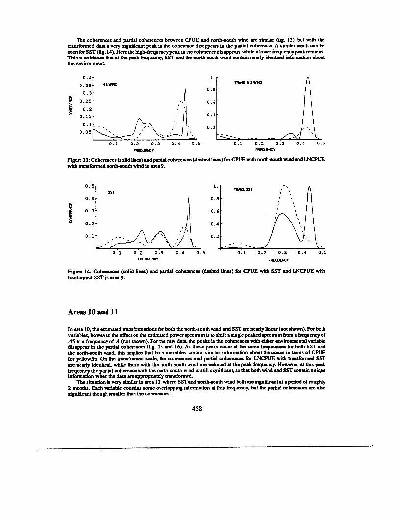
The cohennces and partial cohennces between CPUE and north-south wind me similar (fig. 13). but with the transformed data a v a y signi6cant peak in the cohennccdisappurs in the partial coherence. A similar result can be secnforSST(fig. 14). Henthehigh-hquencypeakinthecoh~dis.ppurs.wvhikabwerhquarcypeakrcm.ins. This is eviduIce that at the peak hqucncy, SST and the north-south wind contain nearly identical infomution about the environment

0.35 0.3.

0.25. Ly

TRANs.KswH) ' N W N o

I 0 . 8 .

0 . 6 . I '

jil 0.1

0 . 4 - 1..

I

0 . 4 .

0.2'

I '

0.1 0.2 0.3 0 . 4 0.5

- _ _ - - - - -

e

TRAM S l ; '\ ' '\

1. f

0.8. I \ ' \

0 . 6 . t

0 .4 '

0.2.

A

0.1 0.2 0.3 0.4 0.5 FREQlEm HEGslcl

Figure 1 4 Cohaencu (solid liner) and partial cohucnces (dashed liner) for CPUE with SST and LNCPUE with trMfOrmedSSTin~9.

Areas 10 and 11

In uw 10. the estimated @ansfonnations for both the north-south wind and SST me nearly linear (not shown). For both variables. however. the effect on the estimated power spectrum is to shift a single puked spectrum h m a kquency of A5 to a frequency of A (not shown). For the raw data, the peaks in the coherences with eitha environmental vuiabk disappear in the partial cohmncu (fig. 15 and 16). As these peaks occur at the same kquenciu for both SST and the north-south wind, this implies that both variables conuin s imi i information about the ocun in terms of CPUE for yellowbn. On the tMsfonned scrk. the coherrnas and partial cohaences for WCPUE with tmasformed SST .TC nearly i d e n t i 4 while those with the north-south wind me rtduced at the peak kquency. However. at this peak frequency the partial cohaence with the north-south wind is still signilicant, so that both wind and SST conuin unique information when the data me appmpriatcly transformed

The situation f very simikr in M 11. where SST and north-south wind both .TC s i g n k t at a paiOa of roughly 2 months. Fhch variabk contains some overlapping information at this frequency, but the partial cohaenccs me also significant though smaller than the cohennces.

458

1.-

0.8

0 . 6 . :: 3 0 . 4 .

0.2.

Ly

Figure IS: Cohuenccs (solid lines) and partial coherences(dashed lines) for CPUE with nonh-south wind and LNCPUE with -formed n o n h - ~ ~ ~ t h wind in area 10.

1.t

’ 0.8.

0.6,

0 . 4 ’

U S w*o TRANS. U S w

1 . -

0.8.

0.6.

0 . 4 .

0 . 2 ’

FRKxlENCV FRMNCT

Figure 1 6 Coherenw (sotid lines) and partial cohmnces (dashed lines) for CPUE with SST and LNCPUE with Iransfonned SST in ales 10.

1.-

0.8’

0.6.

0 . 4 .

0.2’

TRANS. SST

- - - .--

- - - *A-r

SST

e-.

‘ /

Small pelagics off the Ivory Coast

Mendclssohn and Cury (1988) estimate forecasting models and nonlinear annsfonnationS for the explMIltory vrriablcs for modeling the CPUE of small pelagics off the Ivory Coast Mendelsson and Culy (1989) .Is0 study the dominant species in the catch, Surdinello modcredr. in time. as well as in space and time. Their results suggests that the factors affecting the aggregate CPUE arc not the same as those af€ecting S. muderearis by itself. In this section I mxunine this question using the techniques of this paper.

I have a r b h d y estimated the optimal transformations for the explanatory variables from a model which includes lags up to 4 fortnights. Thus. each model contains lagged values of CPUE. Iaggedvaluet of SST at 5 meters depth h n a shore station (SSTSM) and salinity at 5 metus depth (SALSM) from the same sration.

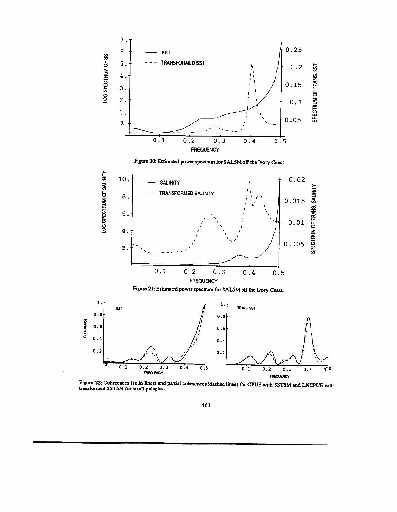
Log of CPUE again is used as the transfoxmation for CPUE. LNCPUE shifts the spectrum from a peak at pound a period of 1 month to a peak centered around 5 w e b (fig. 17). The estimated tnnsformatiom for S n 5 M and S U M (fig. 1 8 . 1 9 ) s ~ t h e i r ~ w ~ ~ ~ i n a s ~ ~ ~ m a n n ~ ~ t h a t a l l ~ ~ haveapeakintheirspecmmatapaiod

The cohaencu and partial cohmnces for SSTSM with CPUE an nearly identical (fig. 22). The cohaences make clear how the transformation has shifted the Sp.ceum so that it is closely aligned with LNCPUE.

The coherencu for CPUE with SALSM show a strong coherence at a period of 1 month. but this disappcan in the partial cohaence (fig. 23). On the transfomed scale. while the coherencu and partial coherrnces arc similar, they arm not particularly significant This supports the claim in Mendclssohn and Cury (1987) that for combined CPUE. SST5M was sufficient for prediction and that no extra information was contained in the SAUM series.

When examining CPUE for S. madrtcnrk only, the picture is diffaent The cohaencts and partial cohennces for SSTSM with CPUE arc nearly identical with a significant peak at a period of roughly 2 months (fig. 24.25). For SALSM. the coherences and partial cohmnces are identical expect at this frequency. where a significant peak in the coherence is eliminated. The most signiticantcoherence for CPUE with S U M is now at a period of roughly a month.

459

of roughly 5 weeks (fig. 2031).

1

'I 1.2 ' I

LOG CPUE ' I ' I

7 . -

6:.

5: I - g

: O - 2

2 .* O S 4 E

- - - - CPUE

0.88 4: 8 3:

* - - - - ' ' - - a 0 . 2 _ _ < - -

1:

Fig-

Oil 0.2 0.3 0.4 0.5 RIECIUENCY

17: Estimated power speceum for CPUE .nd WCPUE for s m d ptgh off the Ivory Cour

v) z -.2

.o .o

'.?. -.4 /' .o +. -.2

2 -.4 -.2 '

- .3

2

20 24 28 20 24 28 20 24 20 20 24 28

SST AT T-1 SST AT T-2 SST AT T-3 SST AT T-4

F@e 18: Estimated transfomurionr for SSTSM off the Ivory Gout.

.10

30 33 36

' 101 ' . --$, .oo

-.20 --lo[

30 33 36

.O . 2 b , , , #--.?;+$, -.2

30 33 36

:::I, .oo , , #..?;r*,

-.lo

-.20 30 33 36

SAL AT T-1 SAL. AT T-2 SAL AT T-3 SAL. AT T-4

Figme 19: Estimated tnnsfonnuions for S U M off the Ivory Cour

7 .* SST 6.-- -

5 . 4 .-. 3 . 2:-

1 . 0. .-c

- - - TRANSFORMED SST -.

-.

-. -.

I - . <'

0.1 0 .2 0.3 0.4 0.5 FREQUENCY

Figure 2 0 Estimated power spectrum for SALSM off the Ivory Coast.

II 'L

- SALINITY

TRANSFORMED SALINITY - - - 8.

6.

4.

2.

0.02

0.015

0.01

0.005

0.1 0.2 0 . 3 0.4 0.5

Figure 21: Estimated power speceum for SAWM off the Ivory Coast FREQUENCY

SST

n

I

c;- - 0.1 0.2 0.3 0 . 4 0.5

FEQIENW

0 . 6 .

0 .4 '

0 . 2 .

\,

0.1 0.2 0.3 0 . 4 0-.!5

Figure 22: CoherenceJ (solid lines) and p d a l cohercnces (dashed lines) for CPUE with SST5M and LNCPUE with transformed SST5M for small pelagics.

46 1

l-1 WJMN 0 .8

1.- 1.

0 . 8 . 0 . 8 ,

0 . 6 .

0 . 4

SST

0 .8 'I -s'-

TRANS. SST -

'

I :::I - ,,-,/ (;;I - ~~. 0.2

_ - 0.1 0.2 0.3 0.4 0.5 0.1 0.2 0.3 0 .4 0.5

"1 WITY 0.8 0.8 l-1 -ssAuwTy

f 0.4 O e 6 I

0 .21

3 0 . 4 0.5 0.1 0 .2 0.3 0 . 4 0.5

FRHXENCY FiEcuem Figwe 25: Cohmncer (solid lines) urd pmtial cohaencer (dashed lines) between raw urd transformed SAWM and raw and transformed CPUE for S. m0dCremi.r.

Thus. for S. m0dCreniC. the p d c o h n c u show SSTSM and S A U M both conuinig significant information about CPUE. but at different frequencies. That SAUM is important for S. muderemu but not for combined CPUE was assated by Mendelssohn and Ctuy (1989) using timedomain techniques. Here I show funha cvidencc of the claim.

The low cohaencer in the transformed data for S. maderenrir is due to the fact that I have Ubiauily used the transformation at 8 lag of 1 formighr Ppdcululy for SAWM. it is clear from the analysis of Mendelsrohn and Cury (1989) that salinity has its prutcst effects at much longer lags. There pc signi6unt urd m c u l t management questions raised by the fact that the dynamics of the combined CPUE (that faced by the &humen) pc much different from that of the dominant specie0 in the utch. Clearly. a forecast of the aggregate could become misleading. and it may be preferable to aggregate foncrpts instead.

462

Long-term memory in the ocean environment in the Gulf of Guinea

Series SST5M

In this section I briefly consider if there is long-term memory in the Ocean environment in the Gulf of Guinea The presence of long-term memory may have profound implications for fisheries management If long-term memoly exists in the ocean. then small changes in the ocean, rather than dying out and causing bounded changes, persist and their effects may multiply through time. Large changes, such as El Nino type events, can have lasting consequences. If the ocean exem a significant influence on the dynamics of a fish population, then it can be expected that fish populations will display a similar property. This would limit how far into the future we can reasonable expect to understand the consequences of managementregimes on the fishery.

I examine the question of the presence of long-term memory by calculating estimates for the fractional differencing parameter d in equations (38) and (39) for several of the environmental series. I use the shore station S S T and salinity series (SSTSM and SALSM) as probably reflecting the environmental conditions relevant to the important near-shore fisheries. I also use SST and the two wind component series from area 9, which is the area of the Intertropical Convergence Zone. This area most likely will reflect much of the dynamics of the Gulf. The salient feature here is that short-term memory series have a value between (-1/2,0), long-term memory models have a value of d between (0,1/2), and series with a value of d greater than 1/2 have infinite variance.

The estimates of d (table 1) suggest that all of the series except the east-west component of the wind have a strong long-term memory component

Method of Estimation Geweke & Porter-Hudak Kashyap & Eom

0.4170 0.4426 SALSM Area 9 SST Area 9 NS Wind

0.4241 0.4486 0.6169 0.6728 0.4036 0.4312 I Area 9 EW Wind I 0.0021 -0.0070 I

Table 1: Estimates of the fractional differencing parameter for selected environmental series in the Gulf of Guinea

There is some evidence that SST may even be an infinite variance series. If this is so. climatologies and other mean-like statistics in this region would have very little meaning. SST in the Gulf of Guinea appears to reflect important processes in the Gulf of Guinea that have major influences on fish dynamics, and my results suggest that these processes may have infinite variance. While much more research must be done in this area before any definitive statements can be made, the initial evidence is troubling indeed.

References

Akaike. H. 1980. On the idenrification of state space models and their use in control. In: D. Brillinger and G. Tim (eds.). Directions In T i e Series. Proceedings of the IMS Special Topics Meeting on Time Series Analysis. Ames. Iowa 1978. Institute of Mathematical Statistics. Hayward.

Anderson.B.D.0. andM.R. Gevm. 1982.Identifiability oflinearstochasticsystemsoperatingun~linear feedback. Automatica. 18:195-213.

Brillinger. David R. 1981. T i e Series: Data Analysis and Theory, (Expanded Edition). San Francisco. Holden-Day.

Breiman. L., and J.H. Friedman. 1985. Estimating optimal transformations for multiple regression and correlation. J. Am. Stat Ass-.. 8 0 580-619.

Caines, P.E. and C.W. Chan. 1975. Feddbackbetween stationary stochastic processes. IEEE Transactions on Auto- matic Control AC-20:498-508.

Cury. P. and C. Roy. 1989. Optimal environmental windows and pelagic fish recruitment success in upwelling ueas. Can. J. Fish. Aquat Sci.. Vol. 46 (4): 670-680.

463

Dempster, A.P.. N.M. Laird and DB. Rubin. (1977). Maximum likelihood from incomplete data via the EM algorithm. J. Roy. Statist Soc.. Ser. B. 39:l-38. Gelfand, I.M. and A.M. Yaglom. 1959. Calculation of the mount of information about a random function contained in another such function. American Mathematical Society Translations, 12 199-246. Gersch. Will. 1986. Modeling multivariate covariance nonstationary time series and their dependent structure. Unpublished manuscript. Dept of Information and Computer Sciences. University of Hawaii.

Geweke. John. 1982. The measurement of linear dependence and feedback between multiple time series. (With discussion). J. Am. Stat Assoc., 77:304-351. Geweke. John. 1984. Measures of conditional linear dependence and feedback between lime series. J. Am. Stat

Geweke. J. and S. Porter-Hudak. 1983. The estimation and application of Long Memory Time Series Models. J. Time Series Anal.. 4221-238. Granger, C.W.G. 1980. Long memory relationships and the aggregation of dynamic models. J. Econometrics. 14:227-238. Granger, C.W.G. and R. Joyeux. 1980. An introduction to long rncmory time series modcls and fractional diffacncing. J. T i e Series Anal.. 1:15-29. Gustafson, I, L. Ljung. and T. SodersWm. 1977. Identification of processes in closed loops - Identifiability and accuracy aspects. Automatica. 1359-75. Hosking. J.R.M. 1981. Fractional differencing. Biometrika. 68:165-176. Hunt, H.E. 1951. Long term storage capacity of resmoirs. Trans. Amer. Soc. Civil. Engrs, 116:770-799. Kashyap. R.L. and Kie-Bum Eom. 1988. Estimation in long-memory time series models. J. Time Series Anal., 9:3542. Lasker. R. 1978. The relation between oceanographicconditions and larval anchovy food in the California Current identification of factors contributing to recruitment failure. Rapp. P.-V. Reun. Cons. I n L Explor. Mer. 173:212-230. Mandelbrot, BB. 1971. A fast Eractional Gaussian noise generator. Water Resources Resurch. 7543-553. Mandelbrot. BB. 1983. The Fractal Geometry of Nature. W.H. Freeman and Company. New Yo&, 4688.

Mandelbrot. BB. and J.W. Van Ness. 1968. Fractional Brownian motion. fractional noises and applications. SL4M Review, 10422-437. Mendelssohn. R. and P. Cury. 1987. Forecasting a formightly abundance index of the Ivoirian coastal pelagic s p i e s and associated environmental conditions. Can. J. Fish. Aquat Sci.. 44:408421.

Mendelssohn. R. and P. Cury. 1989. Temporal and Spatial Dynamics of a Coastal Pelagic Species. Surdinello MderenrkOff the Ivory Coast Can. J. Fish. A q u a Sci, 46(10):1686-1697. Mendelssohn. R. and D. Husby. 1992. Space-Time Analysis and Forecasting of Albacore Catch-per-uniteffort in Relation to the Ocean Environment Manuscript in preparation.

Mendelssohn. R. and C. Roy. 1986. Environmental influenceson the French. Ivory Coast, Senegalaeand Moroccan tuna catches in the gulf of Guinea. p.170-188. in: Special Publication of the International Skipjack Year Program. ICCAT. Madrid.

Mendelssohn. R. and J. Mendo. 1987. Exploratory analysis of anchoveta recruitment off Peru and related e n v h n - mental series. In: D. Pauly and I. Tsukayama (eds.). The Peruvian Anchoveta and Its Upwelling Ecosystem: Three Decades of Change. ICLARM. Manila. p.294-306. Pierce. David A. 1979. Porter-Hudak. Susan L. 1982. Long-Term Memory Modelling - A Simplified Spectral Approach. Ph.D. Thesis. Department of Statistics, University of Wisconsin. Madison.

ASSW., 79:907-915.

measures for time series. J. Am. Stat Assoc.. 7491-910.

Shannon. C.E. 1948. A mathematical theory of communication. Bell Systems Technical Journal, 27379423.623- 656. Shumway. R.H. and DS. Smffer. 1982. An approach to time series smoothing forecasting using the EM algorithm. J. Time Series Anal., 3953-264.

464

Sun& P.N.. M. Blackbum and E Williams. 1981. Tunas rnd their environment in the Pacific ocean: A review. Oceanogr. Mar. Biol. Ann. Rev., 19:443-512.

Uhych. TJ. and T.N. Bishop. 1975. Maximum entropy spectral analysis and autoregressive decomposition. Rev.

Woodward. P.M. 1953. Robability and Information Theory with Applications to Radar. McGraw-Hill. New York.

GeophyS. Space Phys, 13:183-200.

465