33^1 Nonnai^isia do 3Hi QOOld 'NIVId - USGS

:X :** ' *- ^-^,

"' ' : -' I

-a - -

ppuo|j

iuatussassy

'NIVId QOOld ^3Am VICOIhDVIVdV3Hi do Nonnai^isia 33^1

QNV ADOIO^QAH QNV113M

COVER PHOTOGRAPH}

The Landsat image on the cover shows the extent of the flood plain in the Apalaehieola River Basin, Florida. The dark color of the flood plain is caused by the low reflectance from flood waters. The 200-m wide river is barely visible in the center of the 3.2 to 8.0-km- wide flood plain. The Apalaehieola River flows from Lake Seminole (at the top), 171 km south, to Apalaehieola Bay (near the bottom of

the river is pine forest (Apalaehieola National Forest). The faint brown color on the birdsfoot delta at the river mouth is marsh. The

bination of shallow areas and areas with high suspended sediments

The false-color composite was obtained on February 6,1977, by a Landsat multispectral scanner and includes bands 4, 5, and 7. The scene ID is 2746-15190, and more information on this and other satellite images is available through the U.S. Qeologteal Survey, EROS Data Center, Sioux Falls, S. Dak., S7198.

Chapter A

WETLAND HYDROLOGY AND TREE DISTRIBUTION OF THE APALACHICOLA RIVER FLOOD PLAIN, FLORIDA

By HELEN M. LEITMAN, JAMES E. SOHM, and MARVIN A. FRANKLIN

U.S. GEOLOGICAL SURVEY WATER-SUPPLY PAPER 2196

Apalachicola River Quality Assessment

UNITED STATES DEPARTMENT OF THE INTERIOR

WILLIAM P. CLARK, Secretary

GEOLOGICAL SURVEY

Dallas L. Peck, Director

First printing 1984 Second printing 1984

UNITED STATES GOVERNMENT PRINTING OFFICE: 1984

For sale by Distribution Branch Text Products Section U.S. Geological Survey 604 South Pickett Street Alexandria, Virginia 22304

Library of Congress Cataloging in Publication Data

Leitman, Helen M.Wetland hydrology and tree distribution of the Apalachicola

River flood plain, Florida. (Apalachicola River quality assessment) (U.S. Geological Survey water-supply paper ; 2196-A) Bibliography: p.Supt. of Docs, no.: I 19.13.-2196-A 1. Hydrology Florida Apalachicola River flood plain.

2. Wetlands Florida Apalachicola River flood plain.3. Trees Florida Apalachicola River flood plain.4. Flood plain flora Florida Apalachicola River flood plain. I. Sohm, James E. II. Franklin, Marvin A. III. Series. IV. Series: Geological Survey water-supply paper ; 2196-A.

TC801.U2 no. 2196-A [GB705.F5] 553.7'0973s 82-600246[582.16'0526325'0975992]

CONTENTS

List of common and scientific plant names used VII Abstract Al Introduction Al

Purpose and scope Al Acknowledgements A2 Physiography A2 Hydrology and climate A6 Dendrology A7Dams and navigational improvements A8 Land use A9

Methods of investigation A10 Transects A10

Cruise transects A10 Intensive transects A10

Hydrologic methods A14 Surface water A14

Gages A14Flood measurements A14 Step-backwater analysis A14

Ground water A14 Tree sampling A16 Water and tree relations A18

Depth of water A19Fall-season depth A19 Flood depth A19

Duration of inundation and saturation A19Percentage of inundation and saturation A19 Days of inundation and saturation All

Velocity A23 Results and discussion A23

Hydrology A23Surface water A23

Analysis of long-term record A23 The 1980 water year A24River and flood-plain relations at the intensive transects A25

Ground water A28 Trees A30

Species composition A30 Forest types A31

Water and tree relations A34 Depth of water A36

Fall-season depth A36 Flood depth A36

Duration of inundation and saturation A41 Velocity A44

Summary A44 Selected references A46Supplementary data I Transect end points A49 Supplementary data II Description of inundation and saturation conditions

at each transect A49 Conversion factors A52

Contents III

FIGURES

1-3. Maps showing:1. Drainage basin of the Apalachicola, Chattahoochee, and Flint

Rivers in Florida, Georgia, and Alabama A32. Drainage basin of the Apalachicola River in Florida and the

Chipola River in Florida and Alabama A43. Physiography of the Apalachicola River area A5

4. Hydrographs showing river stage at four gaging stations on the Apalachicola River for water year 1980 A7

5. Histogram showing average rainfall in the Apalachicola River basin in Florida compared with that in the basin of the Chattahoochee and Flint Rivers in Georgia A7

6. Profile of altitudes and locations of the 16 dams on the Apalachicola, Chattahoochee, and Flint Rivers A9

7. Aerial photograph showing channel control groins at kilometer 160 on the Apalachicola River A10

8. Aerial photograph showing cutoff of a meander on the Apalachicola River above its confluence with the Chipola River A10

9. Locations of transects and long-term gaging stations shown on a Landsatimage of the Apalachicola River basin All

10, 11. Locations of sampling plots and hydrologic measuring sites shown on an aerial photograph for:

10. Sweetwater intensive transect All11. Brickyard intensive transect A15

12. Photograph showing clump of trees on a hummock at the Brickyard transect between Brickyard Cutoff and Brothers River A16

13. Photographs of a continual-record surface-water gage in the flood plain at plot 12 of the Brickyard transect during the flood and the dry season of 1980 A16

14. Graphs showing relation between step-backwater rating and current-meter rating at Chattahoochee, Blountstown, and Wewahitchka A18

15. Graph showing typical relation between computed and observed flood- plain velocities A19

16. Graph showing stage-discharge relations at the cruise transects A2017. Hydrograph showing 30-day maximum mean discharge and 30-day

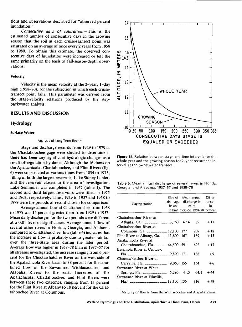
threshold discharge for the 1980 water year at Blountstown A2218. Graph showing relation between stage and time intervals for the whole

year and the growing season for 2-year recurrence interval at the Sweet- water transect A23

19. Graph showing average monthly flows at Chattahoochee, 1929-57 and 1958-79 A24

20. Graphs showing flow and stage duration at Chattahoochee, 1929-57 and 1958-79 A24

21. Graph showing mean monthly flows of the 1980 water year compared with that of the 1958-80 record at Blountstown A25

22. Graph showing percent stage duration for the 1980 water year comparedwith that of the 1958-80 record at Blountstown A25

23, 24. Hydrographs of:23. River stage and flood-plain water levels for the 1980 water year

at the Sweetwater transect A2624. River stage and flood-plain water levels for the 1980 water year

at the Brickyard transect A26

IV Contents

25. Diagram showing flow and velocity distribution at medium and high flood stages at the Sweetwater transect A27

26. Diagram showing flow and velocity distribution at medium and high floodstages at the Brickyard transect A28

27, 28. Hydrographs of:27. Water table and river stage for the 1980 water year at the Sweet-

water transect A2928. Water table and river stage for the 1980 water year at the

Brickyard transect A2929. Photographs of forest types A, B, and E A33

30, 31. Histograms showing:30. Abundance of forest types at each cruise transect A3531. Mean basal area and density of trees of each forest type A36

32. Graph showing mean basal area and density of trees at each cruise transect A36

33. Graphs showing relations between 1979 fall-season water depth and forest type A37

34. Cross sections showing altitude; 2-year, 1-day high (1958-80); and forest type for each cruise-transect point A38

35. Graphs showing relations between 2-year, 1-day high (1958-80) flood depth and forest type A40

36. Graph showing 2-year, 1-day high (1958-80) flood depths at type E forestsat each transect A41

37-38. Graphs showing:37. Relations between percentage of inundation and saturation

(1958-80) and forest type A4238. Relations between consecutive days of inundation and saturation

in the growing season (1958-80) and forest type A4339. Graph showing relation between average velocities during the 2-year, 1-day

high (1958-80) and forest type A44

TABLES

1. The five largest dams in terms of reservoir capacity on the Apalachicola, Chattahoochee, and Flint Rivers A9

2. Cruise-transect names, locations, altitudes, and sampling distances A133. Surface-water gaging stations in the investigation area A174. Ground-water wells at the intensive transects during the 1980 water

year A205. The nine water parameters and associated general hydrologic factors used for

quantifying water and tree relations A216. Mean annual discharge of several rivers in Florida, Georgia, and Alabama,

1937-57 and 1958-78 A237. Maximum mean discharges of Apalachicola River at Blountstown for

specified time periods of 1980 water year, with approximate recurrence inter vals A25

8. Relative importance of tree species on the Apalachicola River flood plain based on cruise-transect data A30

9. Forest types defined at the cruise transects A3110. Relative basal areas of tree species of each forest type, derived from cruise-

transect data A3211. Relative densities of tree species of each forest type, derived from cruise-

transect data A3212. Abundance of forest types at all cruise transects A34

Contents

TABLES Continued

13. Significant correlation coefficients of nine water parameters with each other and river location A37

14. Comparison of relative tolerance of the 12 major flood-plain tree species to inundation and saturation in this investigation to that found under various field and greenhouse situations in the eastern United States A45

VI Contents

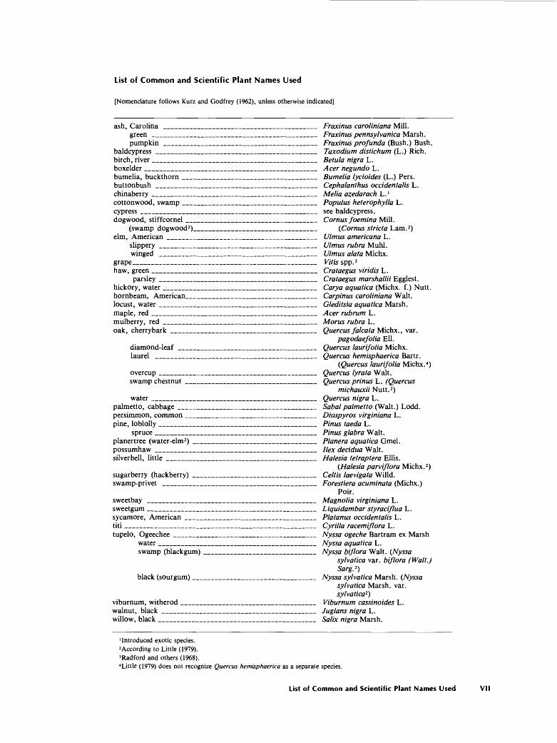
List of Common and Scientific Plant Names Used

[Nomenclature follows Kurz and Godfrey (1962), unless otherwise indicated]

ash, Carolina __________________________ Fraxinus caroliniana Mill.green ____________________________ Fraxinus pennsylvanica Marsh, pumpkin ___________________________ Fraxinus profunda (Bush.) Bush,

baldcypress ___________________________ Taxodium distichum (L.) Rich, birch, river _____________________________ Betula nigra L. boxelder _____________________________ Acer negundo L. bumelia, buckthorn _______________________ Bumetia lycioides (L.) Pers. buttonbush ___________________________ Cephalanthus occidentalis L. chinaberry ____________________________ Melia azedarach L. 1 cottonwood, swamp _______________________ Populus heterophylta L. cypress ______________________________ see baldcypress. dogwood, stiffcornel ______________________ Cornus foemina Mill.

(swamp dogwood2)_____________________ (Cornus stricta Lam. 2) elm, American _________________________ Ulmus americana L.

slippery ____________________________ Ulmus rubra Muhl. winged ___________________________ Ulmus alata Michx.

grape_______________________________ Vitis spp. 3 haw, green ____________________________ Crataegus viridis L.

parsley ___________________________ Crataegus marshallii Egglest. hickory, water __________________________ Carya aquatica (Michx. f.) Nutt. hornbeam, American______________________ Carpinus caroliniana Walt, locust, water ___________________________ Gleditsia aquatica Marsh, maple, red ____________________________ Acer rubrum L. mulberry, red __________________________ Mortis rubra L. oak, cherrybark _________________________ Quercus falcata Michx., var.

pagodaefolia Ell.diamond-leaf _______________________ Quercus laurifolia Michx. laurel ___________________________ Quercus hemisphaerica Bartr.

(Quercus laurifolia Michx. 4 )overcup ___________________________ Quercus lyrata Walt, swamp chestnut ______________________ Quercus prinus L. (Quercus

michauxii Nutt. 2)water ____________________________ Quercus nigra L.

palmetto, cabbage _______________________ Sabal palmetto (Walt.) Lodd. persimmon, common _______________________ Diospyros virginiana L. pine, loblolly ___________________________ Pinus taeda L.

spruce ___________________________ Pinus glabra Walt, planertree (water-elm2) _____________________ Planera aquatica Gmel. possumhaw ___________________________ Ilex decidua Walt, silverbell, little _________________________ Halesia tetraptera Ellis.

(Halesia parviflora Michx. 2 )sugarberry (hackberry) ______________________ Celtis laevigata Willd. swamp-privet __________________________ Forestiera acuminata (Michx.)

Poir.sweetbay _____________________________ Magnolia virginiana L. sweetgum _____________________________ Liquidambar styraciflua L. sycamore, American ______________________ Platanus occidentalis L. titi _________________________________ Cyrilla racemiflora L. tupelo, Ogeechee ________________________ Nyssa ogeche Bartram ex Marsh

water ___________________________ Nyssa aquatica L. swamp (blackgum) ___________________ Nyssa biflora Walt. (Nyssa

sylvatica var. biflora (Walt.) Sarg. 2)

black (sourgum) _____________________ Nyssa sylvatica Marsh. (Nyssasylvatica Marsh, var. sylvatica2)

viburnum, withered _______________________ Viburnum cassinoides L. walnut, black __________________________ Juglans nigra L. willow, black ___________________________ Salix nigra Marsh.

'Introduced exotic species.According to Little (1979).3 Radford and others (1968)."Little (1979) does not recognize Quercus hemisphaerica as a separate species.

List of Common and Scientific Plant Names Used VII

Wetland Hydrology and Tree Distribution of the Apalachicola River Flood Plain, Florida

By Helen M. Leitman, James E. Sohm, and Marvin A. Franklin

Abstract

The Apalachicola River in northwest Florida is part of a three-State drainage basin encompassing 50,800 km 2 in Alabama, Georgia, and Florida. The river is formed by the confluence of the Chattahoochee and Flint Rivers at Jim Woodruff Dam from which it flows 171 km to Apalachicola Bay in the Gulf of Mexico. Its average annual discharge at Chattahoochee, Fla., is 690 m 3/s (1958-80) with annual high flows averaging nearly 3,000 m 3/s. Its flood plain supports 450 km 2 of bottom-land hardwood and tupelo-cypress forests.

The Apalachicola River Quality Assessment focuses on the hydrology and productivity of the flood-plain forest. The purpose of this part of the assessment is to address river and flood-plain hydrology, flood-plain tree species and forest types, and water and tree relations. Seasonal stage fluctuations in the upper river are three times greater than in the lower river. Analysis of long-term streamflow record re vealed that 1958-79 average annual and monthly flows and flow durations were significantly greater than those of 1929-57, probably because of climatic changes. However, stage durations for the later period were equal to or less than those of the earlier period. Height of natural riverbank levees and the size and distribution of breaks in the levees have a major controlling effect on flood-plain hydrology. Thirty-two kilometers upstream of the bay, a flood-plain stream called the Brothers River was commonly under tidal influence during times of low flow in the 1980 water year. At the same distance upstream of the bay, the Apalachicola River was not under tidal influence during the 1980 water year.

Of the 47 species of trees sampled, the five most com mon were wet-site species constituting 62 percent of the total basal area. In order of abundance, they were water tupelo, Ogeechee tupelo, baldcypress, Carolina ash, and swamp tupelo. Other common species were sweetgum, overcup oak, planertree, green ash, water hickory, sugarberry, and diamond-leaf oak. Five forest types were defined on the basis of species predominance by basal area. Biomass in creased downstream and was greatest in forests growing on permanently saturated soils.

Depth of water, duration of inundation and saturation, and water-level fluctuation, but not water velocity, were highly correlated with forest types. Most forest types dominated by tupelo and baldcypress grew on permanently saturated soils that were inundated by flood waters 50 to 90 percent of the time, or an average of 75 to 225 consecutive days during the growing season from 1958 to 1980. Most

forest types dominated by other species grew in areas that were saturated or inundated 5 to 25 percent of the time, or an average of 5 to 40 consecutive days during the growing season from 1958 to 1980. Water and tree relations varied with river location because range in water-level fluctuation and topographic relief in the flood plain diminished downstream.

INTRODUCTION

Forested wetlands are complex transitional systems between terrestrial and aquatic environments. The absorption of high nutrient loads and the diminish- ment of peak flood flows have been recognized as im portant wetland functions. In addition, forested wetlands provide a unique and essential habitat for a diverse assortment of plants and animals (Wharton and others, 1977, p. 335-346). Development pressure in forested flood plains is high, and management con troversies are common. The needed scientific study of forested wetlands is hampered by their complexity and by the limited applicability of conventional limnological or terrestrial ecological techniques.

Purpose and Scope

The Apalachicola River Quality Assessment was initiated in 1978 as part of a national river quality assessment program of the U.S. Geological Survey. The broad objectives and development of the national pro gram were (1) to define the character, interrelations, and apparent cause of existing river-quality problems and (2) to devise and demonstrate the analytical ap proaches and the tools and methodologies needed for developing water-quality information that will provide a sound technical basis for planners and managers to use in assessing river-quality problems and evaluating management alternatives (Greeson, 1978).

The specific goals of the Apalachicola River Quality Assessment conformed to these broad program objectives with the modification that the investigation

Wetland Hydrology and Tree Distribution, Apalachicola Flood Plain, Florida At

was process orientated rather than problem oriented. The Apalachicola River system supports largely un disturbed forested wetlands on the flood plain and highly productive estuaries at its mouth, the Apalachicola Bay. The primary purpose of this assess ment was to investigate river-wetland relations and con trolling factors which influence the yield of nutrients and detritus to the bay. Emphasis was given to processes which influence nutrient and detritus flow, rather than to problems involving environmental disturbance or pollution. Special attention was given to the develop ment of methods because ecological studies of large river-wetland systems have been rare, and few methods particularly applicable to this type of study have been described. The specific goals of the Apalachicola River Quality Assessment were (Mattraw and Elder, 1980):

1. To determine the extent to which potentially toxic trace elements and organic substances accumulate in benthic organisms and sediments.

2. To describe how tree distribution is related to hydrologic conditions in the flood plain.

3. To assess the importance of leaf production and decomposition on the flood plain to detritus and nutrient yields.

4. To identify major sources of nutrients to the river system and quantify transport of nutrients and organic detritus in various parts of the system.

The description of tree distribution and its relation to hydrologic conditions on the Apalachicola River flood plain is the purpose of this report. Three major objec tives of this assessment component were:

1. To observe hydrologic conditions in the forested flood plain and relate them to long-term river- stage record.

2. To estimate species composition and define the major forest types for the flood plain.

3. To relate long-term hydrologic conditions in the flood plain to tree distribution.

Geographically, the Apalachicola River Quality Assessment is limited to the Apalachicola River and its forested flood plain from the confluence of the Chat- tahoochee and Flint Rivers at Jim Woodruff Dam, downstream to Apalachicola Bay. Data collection began in August 1979 and continued through November 1980.

Acknowledgments

The authors wish to acknowledge Ann Redmond of Northwest Florida Water Management District for her assistance in botanical field work in the fall of 1979,

and James Lucas of EROS Data Center for his efforts to interpret hydrologic conditions from satellite images. The following employees of the U.S. Geological Survey are also acknowledged: Linda Geiger for assistance in data interpretation, Gilbert Hughes for analysis of hydrologic record, Sherron Flagg for editing and manuscript preparation, Edwin Malin for illustrations, and numerous other individuals for hydrologic meas urements in the flood of March and April 1980 and other technical support.

Physiography

The Apalachicola River is formed by the con fluence of the Chattahoochee and Flint Rivers (fig. 1). The three rivers drain 50,800 km2 in Georgia, Alabama, and Florida. The Chattahoochee flows about 700 km from its source in north Georgia to Lake Seminole at the Florida-Georgia State line. The Flint River originates south of Atlanta, Ga., and flows about 600 km before it joins the Chattahoochee River. The Apalachicola River is 171 km long and falls about 12m from its head at Jim Woodruff Dam near Chattahoochee, Fla., to the Apalachicola Bay in the Gulf of Mexico (fig. 2). The Apalachicola River downstream from Jim Woodruff Dam drains 6,200 km2 , 50 percent of which is drained by its major tributary, the Chipola River.

The kilometer designations shown in figure 2 are used in this report to indicate locations on the river. They range from kilometer 0 at the U.S. Highway 98 bridge in the city of Apalachicola, to kilometer 171 at Jim Woodruff Dam near Chattahoochee. Kilometers were determined from "navigation miles" established by the U.S. Army Corps of Engineers using the conversion factor of 1.609 kilometers per mile. Locations on the river are marked with prominent signs giving navigation miles. For the convenience of readers, miles are shown in addition to kilometers in figure 2; and conversions from kilometers to navigation miles for each specific river location mentioned are provided in the table of conversion factors in the back of this report.

Figure 3, modified from Puri and Vernon (1964, fig. 5), shows the detailed physiographic regions in the Apalachicola River area. They fall into two broad physiographic categories according to the U.S. Geological Survey (1970, p. 61). The Marianna Lowlands, New Hope Ridge, Greenhead Slope, Foun tain Slope, Grand Ridge, Tallahassee Hills, and Beacon Slope are considered part of the Gulf-Atlantic Rolling Plain. The Coastal Lowlands are part of the Gulf- Atlantic Coastal Flats.

Flood-plain soil has a wide range of textures and colors because it is made up of a variety of sediments that were washed from many different soils. At two locations near Blountstown and Wewahitchka, Leitman

A2 Apalachicola River Quality Assessment

34*

33'

32'

30'

86* 85° 84* 83°

DRAINAGE BASIN OF THE CHATTAHOOCHEE , FLINT, AND

APALACHICOLA RIVERS

GULF OF

MEXICO

Figure 1. Drainage basin of the Apalachicola, Chattahoochee, and Flint Rivers in Florida, Georgia, and Alabama.

Wetland Hydrology and Tree Distribution, Apalachicola Flood Plain, Florida A3

85°30' 85°15' 85°00' 84°45' 84°30'

31°00' i

30°45'

30°30

30°00

29°45'

Figure 2. Drainage basin of the and the Chipola River in Florida Apalachicola River in Florida and Alabama. Kilometer and mile designations indicate specific locations on the Apalachicola River.

EXPLANATION Drainage basin boundaries of

the Apoiachicola and Chipola Rivers

KM 160* KilometersNavigation miles

30°15


GEORGIALOWLAND SM A Rl A N N A

CHATTAHQGCHEE

GAbSDEN'lfCOlJNTY

WAKULLA SAND HILLS

GULF COASTALSAND BAR DUNES

RELICT BAR 8 SPITS

0 10 20 30 KILOMETERS

Figure 3. Physiography of the Apalachicola River area (modified from Puri and Vernon, 1964, fig. 5).


(1978) found flood-plain soils to be predominantly clay with some silty clay and minor clay loam* Sands on point bars were predominantly fine to very fine and were of the micaceous type whereas most Florida sands are siliceous. Cation exchange capacity and organic car bon content were higher than most Florida soils except peats and mucks. The soil pH was acid but not as acid as most Florida soils.

The upper river corridor from Chattahoochee to Blountstown cuts through sediments of Miocene age. Steep bluffs on the east side of the upper river form the western boundary of the Tallahassee Hills physio graphic province (fig. 3), where altitudes are as high as 99 m. The land west of the upper river is gently rolling and rises gradually from the flood plain to the Grand Ridge region where altitudes are as high as 38 m. West of the Grand Ridge area, the land drops slightly to the Marianna Lowlands, a karst plain drained by the Chipola River, the major tributary of the Apalachicola. The flood plain of the upper river is 1.5 to 3 km wide, and the river itself has long, straight reaches and wide, gentle bends. Natural riverbank levees range from 120 to 180 m wide and can be as much as 4.5 m higher than the remainder of the flood plain.

The middle river from Bloutstown to Wewa- hitchka lies in Holocene and Pleistocene deposits. For the first few kilometers, it is bounded on the east by the Beacon Slope physiographic region where altitudes are as high as 45 m. The Gulf Coastal Lowlands, which are below 30 m in altitude, lie to the south and west of the Beacon Slope. The flood plain, wider than that of the upper river, is 3 to 5 km across. The river channel meanders in large loops through the Beacon Slope area and has many small, tight bends further south. Natural riverbank levees range from 60 to 120 m wide and are 2.5 to 4 m higher than the remainder of the flood plain. Dead Lake, just north of Wewahitchka, was formed when natural levees of the Apalachicola River impound ed the Chipola River. According to Vernon (1942), for mation of this lake was due to a much greater sediment load and a more rapid rate of alluviation in the Apalachicola than in the Chipola.

The lower river from Wewahitchka to the city of Apalachicola lies completely in the Gulf Coastal Lowlands with surrounding land-surface altitudes less than 15 m. The Chipola River joins the Apalachicola River at kilometer 45. The flood plain is widest in this section, 4 to 7 km across, and the river is characterized by long straight reaches with a few small bends. Natural riverbank levees range from 15 to 45 m wide and rise 0.5 to 2.5 m above the flood-plain floor. The upstream limit of tidal influence in the flood plain probably does not extend above kilometer 40. Near the city of Apalachicola, the tidal river empties into bays and estuaries bounded by barrier islands and spits (fig. 3).

Hydrology and Climate

The Apalachicola River is 21st in magnitude with reference to discharge of the rivers of the conterminous United States and is the largest river in Florida. The mean annual flow at Chattahoochee from 1958 to 1980 was 690 mVs. The mean annual high was 2,970 mVs, and the mean annual low was 256 mVs. Seasonal fluc tuations in stage (water level in river) and discharge are large. Peak floods are most likely to occur in January, February, March, or April of each year. Low flow generally occurs in September, October, and November. Flood patterns vary greatly from year to year and may not conform to these seasonal trends in any given year.

Fluctuations in stage vary greatly from upper to lower river. Figure 4 shows hydrographs for the 1980 water year at the four long-term gaging stations on the river. At the most upstream station, near the town of Chattahoochee, the stage fell 7.3 m from the peak on March 31, to the low for the year at the end of September, while the stage at the most downstream sta tion, near Sumatra, ranged 2.4 m from the peak to the low.

Georgia rainfall has a greater influence on Apalachicola River flows than Florida rainfall because only 11 percent of the basin of the Apalachicola, Chat tahoochee, and Flint Rivers is in Florida (fig. 1). However, flows in the lower river can be substantially increased by Florida rainfall because of input from the Chipola River near kilometer 45. Flow from the Chipola River averaged 10 percent of the Apalachicola River flow at the Sumatra gage during the 1979 and 1980 water years. Local rainfall can also increase soil satura tion or cause inundation on the flood plain during low or medium river stages, especially in depressions or flat areas having soils with a high percentage of clay.

Average annual rainfall in the Apalachicola River basin in Florida is 1,470 mm (1941-70), and mean an nual potential evapotranspiration is between 990 and 1,140 mm (U.S. Department of Agriculture, 1969). Average annual rainfall in the basin of the Chat tahoochee and Flint Rivers in Georgia is 1,320 mm. Basin rainfall in Georgia is shown with basin rainfall in Florida in figure 5. Georgia rainfall is slightly higher in the winter but much lower in the summer than Florida rainfall. The two States have similar amounts of rainfall in the spring, and both have the least rainfall in October and November (U.S. Department of Commerce, 1973a; 1979a; 1979b).

Mean annual air temperature in the Apalachicola River basin in Florida is 19°C (degrees Celsius). Mean January air temperature is 11°C, and mean July air temperature is 27°C (U.S. Department of Commerce, 1973a). The growing season is from the mean (50 per cent probability) date of the last 0°C frost in the spring


SEA LEVEL

OCT NOV DEC JAN FEB MAR APR MAY JUNE JULY AUG SEPT

1980 WATER YEAR

Figure 4. River stage at four gaging stations on the Apalachicola River for water year 1980.

to the mean date of the first 0°C frost in the fall. The length of the average growing season ranges from 256 days (March 5 to November 15) at the Florida-Georgia State line near Chattahoochee to 281 days (February 23 to November 30) at the Gulf Coast near Apalachicola (J. R. Gallup, National Weather Service, Auburn, Ala., oral commun., 1980).

Dendrology

The forested flood plain of the Apalachicola River is the largest in Florida. It is 114 km long and covers ap proximately 450 km2 (Wharton and others, 1977, p. 70). Of the 211 different species of trees growing in the north Florida area, about 60 are found on the Apalachicola River flood plain. It is dominated by the general forest type, oak-gum-cypress, defined by the U.S. Forest Serv ice as bottom-land forest in which 50 percent or more of the stand is tupelo, sweetgum, oak, and cypress, singly or in combination (U.S. Department of Agriculture, 1969, p. 9). The oak-gum-cypress type is very common on the flood plains of southeastern alluvial rivers; however, this general forest type has been divided into numerous specific types that differ from river to river (Leitman, 1978, p. 6-12).

Z£3

co 20° ac iiih-Ul

1 150_i _iS

-_ 100

if1 50n

-

-

--

- -I 131

^_^

-

-

~

m

-

-

vT]

- 111

1 '

nEXPLANATION

Average rainfall in the Apalachicola River basin in Florida. Rainfall is an average of 30-year normals for 1941-70 for Blountstown and city of Apalachicola.

;rage rainfall in the basin of the Chattahoochee and "lint Rivers in Georgia. Rainfall is an average of :he 30-year normals for the southwest, west central, ind north central divisions. These three divisions :ontain most of the drainage basin of the Chatta-

Ave Fli the 30-yeand north central divisions contain most of the drainr hoochee and Flint Rivers.

Figure 5. Average rainfall in the Apalachicola River basin in Florida compared with that in the basin of the Chat tahoochee and Flint Rivers in Georgia (data from U.S. Department of Commerce, 1973a and b).


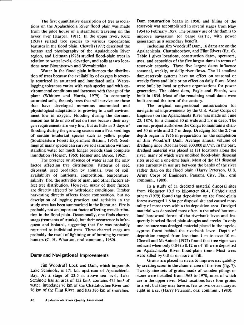
The first quantitative description of tree associa tions on the Apalachicola River flood plain ,was made from the pilot house of a steamboat traveling on the lower river (Harper, 1911). In the upper river, Kurz (1938) related tree species to various topographic features in the flood plain. Clewell (1977) described the botany and physiography of the Apalachicola River region, and Leitman (1978) studied flood-plain trees in relation to water levels, elevation, and soils at two loca tions near Blountstown and Wewahitchka.

Water in the flood plain influences the distribu tion of trees because the availability of oxygen is severe ly restricted in saturated and inundated soils. Water logging tolerance varies with each species and with en vironmental conditions and increases with the age of the plant (Whitlow and Harris, 1979). In constantly saturated soils, the only trees that will survive are those that have developed numerous anatomical and physiological adaptations to growing in a soil environ ment low in oxygen. Flooding during the dormant season has little or no effect on trees because their oxy gen requirements are very low, but as little as 3 days of flooding during the growing season can affect seedlings of certain intolerant species such as yellow poplar (Southeastern Forest Experiment Station, 1958). Seed lings of many species can survive soil saturation without standing water for much longer periods than complete inundation (Hosner, 1960; Hosner and Boyce, 1962).

The presence or absence of water is not the only factor affecting tree distribution. Patterns of seed dispersal, seed predation by animals, type of soil, availability of nutrients, competition, temperature, salinity, fire, the activities of man, and other factors af fect tree distribution. However, many of these factors are directly affected by hydrologic conditions. Timber harvesting directly affects forest composition, but no description of logging practices and activities in the study area has been summarized in the literature. Fire is probably not an important factor affecting tree distribu tion in the flood plain. Occasionally, one finds charred snags (remnants of trunks), but their occurrence is infre quent and isolated, suggesting that fire was probably restricted to individual trees. These charred snags are probably the result of lightning or of burning by racoon hunters (C. H. Wharton, oral commun., 1980).

Dams and Navigational Improvements

Jim Woodruff Lock and Dam, which impounds Lake Seminole, is 171 km upstream of Apalachicola Bay. At a stage of 23.5 m above sea level, Lake Seminole has an area of 152 km2 , contains 475 hm3 of water, inundates 76 km of the Chattahochee River and 76 km of the Flint River, and has 386 km of shoreline.

Dam construction began in 1950, and filling of the reservoir was accomplished in several stages from May 1954 to February 1957. The primary use of the dam is to improve navigation for barge traffic, with power generation as a secondary benefit.

Including Jim Woodruff Dam, 16 dams are on the Apalachicola, Chattahoochee, and Flint Rivers (fig. 6). Table 1 gives locations, construction dates, operators, uses, and capacities of the five largest dams in terms of reservoir capacity. These five largest dams influence seasonal, weekly, or daily river flows. The 11 smallest dam-reservoir systems have no effect on seasonal or weekly flows and little or no effect on daily flows. Most were built by local or private organizations for power generation. The oldest dam, Eagle and Phenix, was built in 1834. Most of the remaining small dams were built around the turn of the century.

The original congressional authorization for navigational improvements by the U.S. Army Corps of Engineers on the Apalachicola River was made on June 23, 1874, for a channel 30 m wide and 1.8 m deep. The current project authorizes the Corps to maintain a chan nel 30 m wide and 2.7 m deep. Dredging for the 2.7-m depth began in 1956 in preparation for the completion of Jim Woodruff Dam. Average annual volume of dredging since 1956 has been 800,000 mVyr. In the past, dredged material was placed at 131 locations along the river, many of which were undiked flood-plain disposal sites used on a one-time basis. Most of the 151 disposal sites currently in use are between the banks of the river rather than on the flood plain (Harry Peterson, U.S. Army Corps of Engineers, Panama City, Fla., oral commun., 1980).

In a study of 11 dredged material disposal sites from kilometer 10.5 to kilometer 68.4, Eichholz and others (1979) found that deposition on the flood-plain forest averaged 1.6 ha per disposal site and caused mor tality of most trees within the deposition area. Dredged material was deposited most often in the mixed bottom land hardwood forest of the riverbank levee and fre quently blocked flood-plain sloughs and creeks. In only one instance was dredged material placed in the tupelo- cypress forest behind the riverbank levee. Depth of deposition ranged from less than 1 m to over 10 m. Clewell and McAninch (1977) found that tree vigor was reduced when only 0.04 to 0.12 m of fill were deposited on Apalachicola River flood-plain trees. Most trees were killed by 0.8 m or more of fill.

Groins are placed in rivers to improve navigability by creating scour in the channel area of the river (fig. 7). Twenty-nine sets of groins made of wooden pilings or stone were installed from 1963 to 1970, most of which are in the upper river. Most locations have four groins in a set, but they may have as few as two or as many as eight in a set (Harry Peterson, oral commun., 1980).


METERS METERS

250

- 200

400 300 DISTANCE, IN KILOMETERS

850 800 700 600 500 400 300 200 100

DISTANCE, IN KILOMETERS

Figure 6. Altitudes and locations of the 16 dams on the Apalachicola, Chattahoochee, and Flint Rivers (modified from U.S. Army Corps of Engineers, 1980).

Table 1. The five largest dams in terms of reservoir capacity on the Apalachicola, Chattahoochee, and Flint Rivers[Data from U.S. Geological Survey, 1977, and U.S. Army Corps of Engineers, 1980]

[Bartlett's Ferry Dam operated by Georgia Power Company; all other dams operated by U.S. Army Corps of Engineers]

Distance up- Dam Reservoir stream of bay,

in km

...... , . Usable reser- Fillmg or pool

. . voir capacity, in completed , ,

nnvPurpose

Buford _______ Sidney Lanier ____ 732 _

West Point ____ West Point ______ 497 _Bartlett's Ferry __ Harding _______ 457 _Walter F. George _ Walter F. George __ 291 _Jim Woodruff ___ Seminole _______ 171 ___

June 1957 ____ 2,079___ Flood control, power, recreation,drinking water.

June 1975 ____ 379 ___ Flood control, power. 1926 _______ 168___ Power.March 1963 ___ 301 ___ Navigation, power, flood control. February 1957 _ 45 ___ Navigation, power.

The U.S. Army Corps of Engineers made four cutoffs in 1956-57 and three more in 1968-69 to straighten bends in the river that were particularly dif ficult for barges to navigate. The cutoffs shortened the total length of the river about 3 km (Harry Peterson, oral commun., 1980). Figure 8 shows the cutoff of a meander, Battle Bend, above the confluence of the Chipola and Apalachicola Rivers.

Land Use

The major land use in the flood plain is forestry. Most areas were first cut between 1870 and 1925

(Clewell, 1977, p. 11) and have been logged once or twice since that time. Regrowth has been rapid, and much of the flood plain has the general aspect of a mature forest. Other extensive uses are beekeeping for tupelo honey production, commercial and sport fishing, and hunting. A few areas on the flood plain have been cleared for agriculture (row crops and improved pasture) and residential developments. Population and development in the area are relatively sparse.

Most of the flood plain is owned by lumber and paper companies and is managed for timber harvesting. A large part of the flood plain in the lower reaches of the river is publicly owned. In 1977-78, the State of Florida Environmentally Endangered Lands Program


^^f*fe£&r^

Figure 7. Aerial photograph showing channel control groins at kilometer 160 on the Apalachicola River. Groins are 30 to 100 m in length.

purchased 113 km2 of flood plain from about kilometer 34 to Apalachicola Bay. According to Florida statutes, land below the "ordinary high water line" of the river is owned by the State.

METHODS OF INVESTIGATION

Transects

Cruise Transects

Eight transects were established across the Apalachicola River flood plain to collect data on water depth, duration, and velocity, and tree cover and densi ty. The transects were located perpendicular to the flood-plain corridor at approximately equally spaced in tervals from the dam at Chattahoochee to the south end of Forbes Island in the lower river. Transect and long- term gage locations are shown in figure 9.

Cruise-transect points were established at 90-m in tervals across each transect. Limited amounts of water and tree data were collected at these points, once in the autumn of 1979 and once in the spring of 1980. The methods by which these data were collected are called "cruise transect" methods because they are similar to timber cruising methods used by foresters. Specific tree- sampling and hydrologic methods are described in subsequent sections. Cruise-transect names, locations, altitudes, and sampling distances are given in table 2. The transects did not extend the full width of the flood plain due to unclear flood-plain boundaries, alterations

Figure 8. Aerial photograph showing cutoff of a meander on the Apalachicola River above its confluence with the Chipola River.

by man, and project time constraints. Supplementary Data I (p. A49) describes the end points of each transect.

Intensive Transects

At the Sweet water and Brickyard transects, many additional water and tree observations were made dur ing the 2-year period of investigation. The methods by which these additional data were collected are called "in tensive transect" methods because the variety of data and frequency of collection were much greater than those of the cruise-transect methods. Intensive transects were located as close as possible to the long-term gaging stations at Blountstown and Sumatra. Tree and water observations were made at 16 sampling plots of 500 m2 each (7 at Sweetwater and 9 at Brickyard) in addition to the numerous cruise-transect sampling points listed in table 2. Sampling plot design, tree-sampling, and hydrologic methods for the intensive transects are described in subsequent sections.

The Sweetwater intensive transect is located about 10.5 km upstream of U.S. Highway 20 bridge near Blountstown. Figure 10 shows the location of sampling plots and hydrologic measuring sites. Immediately east of plot 1, there is a steep bluff rising 45 m higher than the flood plain. This is part of a continuous steep bluff and ravine system on the east side of the flood plainFigure 9 (right). Locations of transects and long-term gaging stations shown on a false-color composite of Landsat multispectral scanner bands 4, 5, and 7; the image (2746-15190) was acquired Feb. 6,1977.


Sl .*W^ «

Torreya Park

iweetwater'-H-H

Blountstown Gage River

Muscogee Reach

Porter Lake

' Wewahilchka GageA

EXPLANATION Cruise transect

only

MM Intensive and cruise transects

A Long-termcontinual - record gagin

Brickyard Sumatra Gage

South end, Forbes Island

5 1O 15 KILOMETERS


Table 2. Cruise-transect names, locations, altitudes, and sampling distances

Transect name

Upper River: ChattahoocheeTorreya ParkSweetwater 1

Middle River: Old RiverMuscogee ReachPorter Lake

Lower River: Brickyard 1South end of Forbes Island

Total

River location,

in km

168.5150.1138.1

116.5. _ 98.0

78.5

32.320.1

Altitude iMinimum, excluding

stream beds

15.514.313.5

10.87.75.5

0.3.5

n meters

Maximum

20.117.918.1

15.111.39.5

3.52.3

Number of sampling

points

201227

362816

4539

223

Length of transect, in meters

1,8001,100

22,400

3,2002,500

3 1,500

4,10043,50020,100

1 Sampled by intensive-transect methods also.2Water depths and velocities were taken for an additional 730 m to the west. 3An additional 3,300 m on the east side not sampled due to recent logging. "Water depths and velocities were taken for an additional 2,100 m to the east.

24

co a: LU

LU OIDtie

12

B

WEST EAST

Ground Surface

0 100 200

DISTANCE FROM PLOT 1, IN METERS

Figure 10. A (left), Locations of sampling plots and hydrologic measuring sites, Sweetwater intensive transect, shown on a color-infrared aerial photograph acquired Nov. 15,1979, by National Aeronautics and Space Administration. B (above), Sectional view of plot 1.

from Chattahoochee to Bristol. The flood plain from plot 1 to plot 2 is very flat with soft organic mud that is always covered with about a half meter of water. West of this ponded area, the land rises to a high natural levee of firm, sandy loam at plot 4. No well-defined streams exist on the east flood plain.

A stream on the west flood plain begins near the transect at the river bank, flows north, returns to the south and crosses the transect line at plot 7. Plots 5 and 6 have firm, loamy clay soils that are infrequently flood ed. Plot 7 is on a low silty stream bank that is frequently flooded. Immediately to the west of plot 7 is a recently cleared brushy area which gradually rises westward to a road that is less than 3 m above the west flood plain. No plots were located in this area because of the lack of trees; however, discharge measurements were made here during the March and April 1980 flood. The upland region for 3 km west of the transect is 3 to 9 m higher than the west flood plain.

Figure 11 shows the location of sampling plots and hydrologic measuring sites at the Brickyard inten sive transect. The upland to the east ranges from 2 to 4 m higher than the flood plain. No flood plain exists east of the river. The transect lies parallel to, and about 100 m south of, the Florida Power Corporation powerline crossing. During powerline construction, trees were cleared from the crossing area, but use of earth-moving equipment was limited. Consequently, ground levels in the powerline clearing are not significantly different than the surrounding area, and effects of the powerline or its construction on water movement in the flood plain were undetectable.


Brickyard Cutoff and the Brothers River divide this transect into three areas. Sample plots 11, 12, 13, and 14 are between the Apalachicola River and Brickyard Cutoff on Forbes Island. Plots 11 and 14 lie on narrow natural levees surrounding a very large, flat, and muddy area of saturated clays. Between Brickyard Cutoff and the Brothers River the land rises to a firm hummock around nearly every tree or group of trees (fig. 12). The land between hummocks is riddled with shallow sloughs having soupy mud bottoms. Plot 15 is on the east side of a deeper slough (1.2 m deep during low water) that connects to the Brothers River about 300 -m north of the powerline. The flood plain west of the Brothers River (plots 18 and 19) is mostly flat with clayey muds. The transect ends at a manmade levee. For 5 km west of this levee, ground levels are 0 to 2 m higher than the flood plain.

Hydrologic Methods

Surface Water

Gages

Four long-term (fig. 9) and four project continual- record gaging stations (figs. 10 and 11) within the area of investigation provided stage and discharge informa tion for this report. The gages are listed in table 3 with station name and number, period of record, type of data, and location. Figure 13 shows the project gage in the flood plain at plot 12 of the Brickyard transect dur ing and after the March and April 1980 flood.

An effort was made to fill in periods of in complete or missing record at the long-term gages. Daily discharge for the period 1922-57, at Blountstown, was computed by developing a stage-discharge relation from miscellaneous discharge measurements. The relation is well defined from discharge measurements between 150 and 2,800 mVs, and is extended above 2,800 mVs using the stage-discharge relation for the period 1958-80. The stage-discharge relation at Wewahitchka is good within bank-full stage. This relation was extrapolated to high flow by step-backwater analysis. From this relation, daily discharge was computed for the period 1965-80. The stage-discharge relation at Sumatra was used to compute the daily discharge for the period 1950-59. For 1959-77, the daily discharge was estimated by adding the daily discharge from the Apalachicola River near Blountstown and the Chipola River near Altha and lag ging the total by 3 days. When compared to periods of actual record, daily discharge estimated by this method indicated a correlation coefficient of 0.92.

Flood Measurements

During the March and April 1980 flood, repeated discharge measurements were made across the Sweet-

water and Brickyard transects. Particular attention was devoted to the sample plots, with detailed visual obser vations to note any changes in the physical surround ings. Water depth and velocity were measured once dur ing the flood at each cruise transect point.

Step-Backwater Analysis

Stage-discharge relations were available at the four long-term gaging stations on the Apalachicola River before the March flood. During the flood, a par tial rating for the Sweet water transect was developed. In order to develop a rating at the cruise transects, a step- backwater analysis was performed (Shearman, 1976, fig. 2).

The U.S. Geological Survey gage near Sumatra provided the known stage-discharge relation. The U.S. Army Corps of Engineers furnished cross sections for the main channel. Gee and Jenson Engineers, Inc., fur nished several flood-plain cross sections in Gulf, Franklin, and part of Liberty Counties. The Florida Department of Transportation furnished cross sections at road crossings. Cross sections for the cruise transects were determined during the flood by measuring from the known water surface to the ground at previously established points. All cross sections were plotted, and the distance between each was determined. The roughness coefficient (Manning's ri) was estimated from field observations and aerial photographs.

The step-backwater analysis used to generate the water-surface profiles employs measured values with the exception of Manning's n. Estimated n values were calibrated by comparing stage-discharge relations for Wewahitchka, Blountstown, and Chattahoochee to the computed profiles (fig. 14). Distribution of flow in the flood plain was checked by comparing velocity observa tions made in the flood plain during the March flood to the velocities computed by step-backwater analysis in each subarea for which observed velocities were avail able (fig. 15). The analysis was used to generate stage- discharge and stage-velocity relations at the transects. Figure 16 is the final stage-discharge relation for each of the transects after the n values were calibrated.

Ground Water

In order to study the relation of ground water and surface water within the intensive transects of the study area, a network of ground-water observation wells was constructed (table 4, figs. 10 and 11). Two wells at each intensive transect provided a continual record of water- table fluctuations in response to river-stage changes.

Figure 11 (right). Locations of sampling plots and hydrologic measuring sites, Brickyard intensive transect, shown on a color-infrared aerial photograph acquired Nov. 15, 1979, by National Aeronautics and Space Administration.


Monthly measurements of the water table were made at several additional wells both in and out of. the flood plain at both transects.

Tree Sampling

An accurate characterization of tree species at each intensive-transect plot was necessary to correlate with the detailed hydrologic information collected. To determine the appropriate plot size, a nested-plot test was conducted at each transect. The purpose of a nested-plot test was to determine the smallest area on which the species composition of the forest type in ques tion was adequately represented (Mueller-Dombois and Ellenberg, 1974, p. 47-50). As a result of these tests, 500 m2 was estimated as the optimum plot size. Forest types apparent on aerial photographs were located and checked in the field. At least one 500-m2 plot was located in each forest type, and plot boundaries were marked with string. Seven plots were located at the Sweetwater transect and nine at the Brickyard transect (figs. 10 and 11). The genus, species, diameter, and crown class of each tree, 75 mm or greater in diameter, were recorded for each plot. Nomenclature follows Kurz and Godfrey (1962). Diameters were measured at breast height, 1.4 m above ground. Buttressed, forked, or deformed trees were measured according to Avery (1967, p. 74). Trees less than 75 mm in diameter were not measured because they did not meet the minimum

Figure 12. Clump of trees on a hummock at the Brickyard transect between Brickyard Cutoff and Brothers River. This hummock rises about 1 m above the water surface.

A BFigure 13. Continual-record surface-water gage in the flood plain at plot 12 of the Brickyard transect, (A) during the flood of March and April 1980 and (6) during a dry fall season in December 1980. Arrow in photograph B indicates water level during the flood in photograph A.


Table 3. Surface-water gaging stations in the investigation area

Station name and number 1

LocationPeriod of

recordType of record

Apalachicola River atChattahoochee, 02358000.

Sweetwater plot 1, 302851084590500.

Sweetwater plot 7, 302849085004200.

Apalachicola River near Blountstown, 02358700.

Do_______

On downstream side of right main pier on U.S. High way 90, 1.0 km downstream from Jim Woodruff Dam, and 1.6 km west of Chattahoochee.

In flood plain near east end of the Sweetwater inten sive transect 10.5 km north of Bristol.

In flood plain near west end of the Sweetwater inten sive transect 10.5 km north of Bristol.

On the right bank 152 m upstream from Neal Lum ber Company Landing, 2.4 km southeast of Blountstown.

.do.

1928 to 1980 Mean daily discharge.

Apalachicola River near Wewahitchka, 02358754.

Apalachicola Rivernear Sumatra, 02359170.

Do-___________

On the right bank just above the Chipola Cutoff, 5.5 km east of Wewahitchka.

09-20-79 to

09-30-80

10-10-79to

09-30-80

1920 to 1957

1958 to 1980

1965 to 1980

On left bank at Brickyard Landing, 3.9 km west of 1950 to 1959 Fort Gadsden and 8.5 km southwest of Sumatra.

-do

Brickyard plot 12, 295621085011500.

Brothers River,295610085024500.

09-09-77to

09-30-80

In flood plain, between Apalachicola River and 10-05-79 Brickyard Cutoff at Brickyard intensive transect. to

09-30-80

On the left bank of Brothers River about 61 m north of the Brickyard intensive transect.

10-01-79to

09-30-80

Mean daily stage.

Mean daily stage.

Once daily stage and occasional discharge.

Mean daily discharge.

Mean daily stage and occasional discharge.

Mean daily stage and occasional discharge.

Mean daily discharge.

Mean daily stage.

Mean daily stage.

'Station identification number.

dimensions of a tree according to Kurz and Godfrey (1962, p. XIV). Four crown classes (dominant, codomi- nant, intermediate, and overtopped) were used as de fined by Avery (1967, p. 212).

Cruise transects were sampled at 90-m intervals by the point-sampling method. Distances were measured by pacing, and a compass was used to determine direc tion. The tree nearest each point was marked with dou ble flagging, and the transect line between each point was marked with single flagging. Sampling at each point was done with a glass wedge prism (Avery, 1967, p. 165-183; Kulow, 1965). Prism sampling is more effi cient than plot sampling when characterizing the signifi cant species over a very large area because the largest

trees and most frequently occurring trees are sampled much more than the small and uncommon trees. Genus, species, diameter, and crown class were recorded for each tree. One important difference between the plot and point methods was the minimum diameter. Plot sampling measured only those trees 75 mm or greater in diameter. No minimum diameter limit was used for point sampling.

Upon completion of tree sampling, basal area (cross-sectional stem area) and density (number of trees) were calcuated for each tree species at each plot and point (Avery, 1967). Relative basal area and density were also calculated. Relative basal area is the percen tage of the total basal area comprised by each species.


CO IT UJr- UJ

UJo

APALACHICOLA RIVER NEAR CHATTAHOOCHEE

5

4.5

I__I

EXPLANATION

EXISTING RATING

STEP-BACKWATER RATING

APALACHICOLA RIVER NEAR WEWAHITCHKA

i i i i i i200 500 1000 2000 5000 200

APALACHICOLA RIVER NEAR BLOUNTSTOWN

1000 2000 5000

DISCHARGE, IN CUBIC METERS PER SECOND

Figure 14. Relation between step-backwater rating and current-meter rating at Chattahoochee, Blountstown, and Wewahitchka.

Relative density is the percentage of total density com prised by each species.

Tree species were grouped into five forest types designated A through E on the basis of species predom inance by basal area, using a method of classifying vegetation that is similar to the tabular comparison method described by Mueller-Dombois and Ellenberg (1974, p. 177-210). "Forest Cover Types of United States and Canada" (Eyre, 1980) was used as a guide for naming the types.

Water And Tree Relations

For each of the 223 cruise-transect points, nine hydrologic parameters in three general categories were quantified (table 5). Depth of water was measured dur ing both dry and flooded conditions. Duration of inun dation and saturation in the flood plain was estimated with six different parameters. Velocity was measured only during flooded conditions. Water parameters at each cruise-transect point were grouped by forest type


19

18

(O CC.UJh- UJ

UJoID

17

16

15

14

EXPLANATION

A OBSERVED MEAN VELOCITY X COMPUTED VELOCITY

0 0.1 0.2 0.3 0.4 0.5VELOCITY, IN METERS

PER SECONDFigure 15. Typical relation between computed and ob served flood-plain velocities. Measurements shown were taken on the west flood plain of the Sweetwater transect.

to determine the relation between tree communities and water regimes.

Depth of Water

Fall-Season Depth

Fall-season depth is the water present at each cruise-transect point during the low-water or drier period of the year. If standing water was present, the water depth was reported as a negative number (that is, - 1.0 = 1m deep). If no standing water was present, soil moisture was judged by appearance on the surface as dry, damp, or saturated. According to Frevert and others (1955, p. 90-92), when the soil appears saturated, all pore space is filled with water and the soil moisture potential is zero. Damp soils are between field capacity and wilting point. Soils that appear dry have reached or surpassed the wilting point. Fall-season depth at each site was observed in November and early December

1979. Rainfall was negligible during that period, but minor flooding was a problem in late November and early December in the lower river. Therefore, fall- season depth observations were repeated at some loca tions in the fall of 1980.

Flood Depth

Flood depth is the depth of water at each cruise- transect point during the 2-year (0.5 probability), 1-day high (1958-80). The 2-year, 1-day high was used because it is the average annual flood. Water depths are reported as negative numbers. If a point remained dry during the 2-year, 1-day high, the distance of the ground above the water level of the 2-year, 1-day high is reported as a positive number.

The following steps were taken to obtain flood depths. Water depths at each point were taken on various dates during the March and April 1980 flood when river stage was high enough to assume a level water surface across the flood plain. Distance to the water surface was measured from one reference point at each transect on the same day that depths were taken. Altitude of the reference point was determined by surveying from benchmarks. Water depths were then subtracted from the altitude of the water surface to ob tain the altitude of the ground at each point. Frequency analyses were performed on long-term gage record (1958-80) to determine the discharge of the 2-year, 1-day high. Rating curves developed by the step- backwater analysis were used to determine the altitude of the 2-year, 1-day high at each transect. Altitudes of the ground at each point were subtracted from altitudes of the 2-year, 1-day high at each transect to obtain flood depths.

Duration of Inundation and Saturation

Percentage of Inundation and Saturation

Percentage of inundation estimated from river- stage record. Percentage of inundation estimated from river-stage record is the total percentage of time from 1958 to 1980 that river stage equaled or exceeded the ground level of each cruise-transect point. This parameter is derived from stage-duration curves at the cruise transects which were interpolated from 1958-80 flow-duration curves at Chattahoochee, Blountstown, and Sumatra and from 1965-80 curves at Wewahitchka through the use of stage-discharge rating curves. This parameter is known to be unrepresentative at some loca tions because of differences in stage between the river and flood plain where flow between the two is retarded by natural levees or other features. Duration of inunda tion in the flood plain, therefore, may be shorter or longer than the duration of flooding above a given stage in the river. Despite its inadequacies, river-stage record


^ South end Forbes Island

2000 3000

DISCHARGE, IN CUBIC METERS PER SECOND

Figure 16. Stage-discharge relations at the cruise transects.

4000

Table 4. Ground-water wells at the intensive transects during the 1980 water year

Location

About 170 m east of plot 1, on upland at east end of Sweetwater transectAbout 100 m east of plot 1, at base of steep bank at east end of Sweetwater

transectAbout 80 m east of plot 1, in flood plain at east end of Sweetwater transect ___ At plot 3 on Sweetwater transect, about 30 m west of permanent pond cover

ing most of the east flood plainAt plot 4 on Sweetwater transect, about 120 m east of Apalachicola River ____ At plot 7 on west end of Sweetwater transect, in a flood-plain streamAt Brickyard Landing, about 60 m east of Apalachicola River and 15m north

of landing roadNear plot 1 1 on Brickyard transect, on the natural riverbank levee about 30 m

west of the Apalachicola RiverAt plot 12 on Brickyard transect, in the interior of Forbes IslandAt plot 15 on Brickyard transect, near a slough between Brickyard Cutoff and

Brothers RiverAt plot 16 on Brickyard transect, between Brickyard Cutoff and Brothers

River about 300 m west of plot 15

Type of record

Monthly

MonthlyMean daily

MonthlyMean daily Monthly

Monthly

Mean dailyMean daily

Monthly

Monthly

Altitude of land surface,

in meters

22

1614

1515 14

4.3

1.71.1

0.6

0.9

Depth of well below

land surface, in meters

4.6

0.54.0

2.74.6 2.4

4.3

1.82.4

3.7

3.7


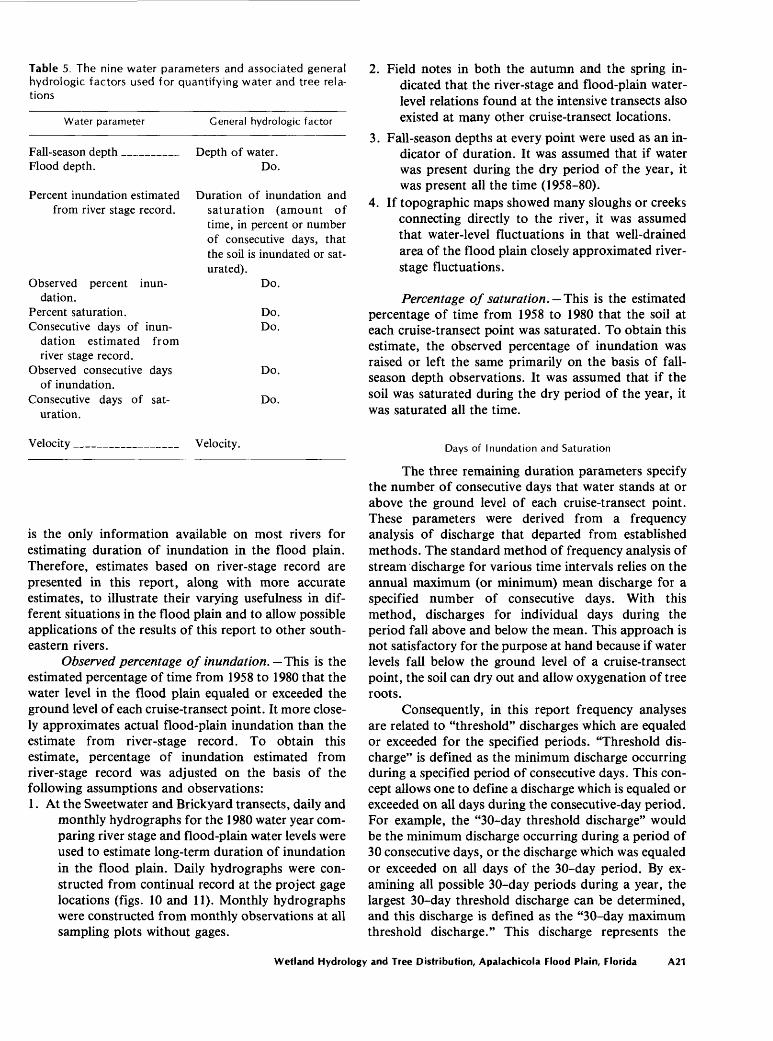
Table 5. The nine water parameters and associated general hydrologic factors used for quantifying water and tree rela tions

Water parameter General hydrologic factor

Fall-season depth Flood depth.

Percent inundation estimated from river stage record.

Observed percent inun dation.

Percent saturation.Consecutive days of inun

dation estimated from river stage record.

Observed consecutive days of inundation.

Consecutive days of sat uration.

Velocity ___________ Velocity.

Depth of water. Do.

Duration of inundation and saturation (amount of time, in percent or number of consecutive days, that the soil is inundated or sat urated).

Do.

Do. Do.

Do.

Do.

is the only information available on most rivers for estimating duration of inundation in the flood plain. Therefore, estimates based on river-stage record are presented in this report, along with more accurate estimates, to illustrate their varying usefulness in dif ferent situations in the flood plain and to allow possible applications of the results of this report to other south eastern rivers.

Observed percentage of inundation. This is the estimated percentage of time from 1958 to 1980 that the water level in the flood plain equaled or exceeded the ground level of each cruise-transect point. It more close ly approximates actual flood-plain inundation than the estimate from river-stage record. To obtain this estimate, percentage of inundation estimated from river-stage record was adjusted on the basis of the following assumptions and observations: 1. At the Sweet water and Brickyard transects, daily and

monthly hydrographs for the 1980 water year com paring river stage and flood-plain water levels were used to estimate long-term duration of inundation in the flood plain. Daily hydrographs were con structed from continual record at the project gage locations (figs. 10 and 11). Monthly hydrographs were constructed from monthly observations at all sampling plots without gages.

2. Field notes in both the autumn and the spring in dicated that the river-stage and flood-plain water- level relations found at the intensive transects also existed at many other cruise-transect locations.

3. Fall-season depths at every point were used as an in dicator of duration. It was assumed that if water was present during the dry period of the year, it was present all the time (1958-80).

4. If topographic maps showed many sloughs or creeks connecting directly to the river, it was assumed that water-level fluctuations in that well-drained area of the flood plain closely approximated river- stage fluctuations.

Percentage of saturation. This is the estimated percentage of time from 1958 to 1980 that the soil at each cruise-transect point was saturated. To obtain this estimate, the observed percentage of inundation was raised or left the same primarily on the basis of fall- season depth observations. It was assumed that if the soil was saturated during the dry period of the year, it was saturated all the time.

Days of Inundation and Saturation

The three remaining duration parameters specify the number of consecutive days that water stands at or above the ground level of each cruise-transect point. These parameters were derived from a frequency analysis of discharge that departed from established methods. The standard method of frequency analysis of stream discharge for various time intervals relies on the annual maximum (or minimum) mean discharge for a specified number of consecutive days. With this method, discharges for individual days during the period fall above and below the mean. This approach is not satisfactory for the purpose at hand because if water levels fall below the ground level of a cruise-transect point, the soil can dry out and allow oxygenation of tree roots.

Consequently, in this report frequency analyses are related to "threshold" discharges which are equaled or exceeded for the specified periods. "Threshold dis charge" is defined as the minimum discharge occurring during a specified period of consecutive days. This con cept allows one to define a discharge which is equaled or exceeded on all days during the consecutive-day period. For example, the "30-day threshold discharge" would be the minimum discharge occurring during a period of 30 consecutive days, or the discharge which was equaled or exceeded on all days of the 30-day period. By ex amining all possible 30-day periods during a year, the largest 30-day threshold discharge can be determined, and this discharge is defined as the "30-day maximum threshold discharge." This discharge represents the


10000P

MEAN 2300 THRESHOLD 1,800 ~~


1980 WATER YEAR

Figure 17. Thirty-day maximum mean discharge and 30-day threshold discharge for the 1980 water year at Blountstown.

largest discharge which was equaled or exceeded for 30 consecutive days during the year. Similarily, this con cept can be applied to any other consecutive day period, such as a 3-day, 7-day, or 15-day period. The max imum threshold discharge can be converted to a water level by using a stage-discharge relation.

The 30-day maximum threshold discharge is com pared to the 30-day maximum mean discharge at Blountstown during the 1980 water year (fig. 17). The 30-day maximum mean discharge is 2,300 mVs, whereas the 30-day maximum threshold discharge of 1,800 mVs is the highest discharge that was equaled or exceeded for 30 consecutive days during the 1980 water year.

The maximum threshold discharge for various time intervals (1, 7, 30, 60, 90, 120, 183, and 365 con secutive days) was determined from hydrographs for each of the water years 1958-80 at the Chattahoochee, Blountstown, and Sumatra gages and 1965-80 at the Wewahitchka gage. A log-Pearson Type III frequency analysis (U.S. Water Resources Council, 1977) was per formed for each of the time intervals. From this array of frequency curves a relation between discharge and time intervals was established for a 2-year recurrence interval (0.5 probability) for each of the long-term gages. By in terpolation of the long-term gage data, similar relations were established for each transect. Stage-discharge rela tions developed by the step-backwater process were available for converting the discharge-time interval rela tion to a river stage-time interval relation for the 2-year recurrence interval for each transect.

Flooding during the dormant season usually has no effect on trees (Hall and Smith, 1955, p. 283-284; McAlpine, 1961, p. 567; Yelenosky, 1964, p. 140). The average growing season for the Apalachicola River is 266 days from March 1 through November 21 (J. R. Gallup, National Weather Service, Auburn, Ala.; oral commun., 1980); therefore, days of flooding from November 22 to February 28 are not important to tree

growth and survival. Consequently, maximum thresh old discharges and stage-time interval relations were determined for each transect for the growing season in the manner previously described for complete water years. The stage-time interval relation for the 2-year recurrence interval at Sweetwater intensive transect is shown in figure 18 for both the complete water year and the 266-day growing season. Water parameters follow ing in this section use only the growing season relations.

Consecutive days of inundation estimated from river-stage record. This is the number of consecutive days in the growing season that river stage equaled or exceeded the ground level of each cruise-transect point on an average of once every 2 years from 1958 to 1980. To estimate this parameter at each cruise-transect point, the altitude of the ground level was located on the left axis in figure 18, and the number of days inundated was read from the growing season curve. In the example shown by the dashed lines, a cruise-transect point at Sweetwater transect having an altitude of 14.6 m was in undated 20 consecutive days in the growing season on the average of once every 2 years (0.5 probability) from 1958 to 1980. This parameter is known to be unrepre sentative at some locations because of differences in stage between the river and flood plain where flow be tween the two is retarded by natural levees or other features. Days of inundation in the flood plain, therefore, may be more or less than the days of flooding above a given stage in the river.

Observed consecutive days of inundation. This is the estimated number of consecutive days in the grow ing season that the water level in the flood plain equaled or exceeded the ground level of each cruise-transect point on an average of once every 2 years from 1958 to 1980. It more closely approximates consecutive days of inundation at each point than the river-stage estimate just described. To obtain this value, consecutive days of inundation estimated from river-stage record were ad justed on the basis of combinations of the four assump-


tions and observations described for "observed percent inundation."

Consecutive days of saturation. This is the estimated number of consecutive days in the growing season that the soil at each cruise-transect point was saturated on an average of once every 2 years from 1958 to 1980. To obtain this estimate, the observed con secutive days of inundation were increased or left the same primarily on the basis of fall-season-depth obser vations.

Velocity

Velocity is the mean velocity at the 2-year, 1-day high (1958-80), for the subsection in which each cruise- transect point falls. This parameter was derived from the stage-velocity relations produced by the step- backwater analysis.

RESULTS AND DISCUSSION

Hydrology

Surface Water

Analysis of Long-Term Record

Stage and discharge records from 1929 to 1979 at the Chattahoochee gage were studied to determine if there had been any significant hydrologic changes as a result of regulation by dams. Although the 16 dams on the Apalachicola, Chattahoochee, and Flint Rivers (fig. 6) were constructed at various times from 1834 to 1975, filling of both the largest reservoir, Lake Sidney Lanier, and the reservoir closest to the area of investigation, Lake Seminole, was completed in 1957 (table 1). The second and third largest reservoirs were filled in 1975 and 1963, respectively. Thus, 1929 to 1957 and 1958 to 1979 were the periods of record chosen for comparison.

Average annual flow at Chattahoochee from 1958 to 1979 was 15 percent greater than from 1929 to 1957. Mean daily discharges for the two periods were different at a 0.01 level of significance. Average annual flow of several other rivers in Florida, Georgia, and Alabama compared to Chattahoochee flow (table 6) indicates that the increase in flow is probably due to greater rainfall over the three-State area during the later period. Average flow was higher in 1958-78 than in 1937-57 for all streams investigated, the increase ranging from 6 per cent for the Choctawhatchee River on the west side of the Apalachicola River basin to 38 percent for the com bined flow of the Suwannee, Withlacoochee, and Alapaha Rivers to the east. Increases of the Apalachicola, Chattahoochee, and Flint Rivers were between these two extremes, ranging from 13 percent for the Flint River at Albany to 18 percent for the Chat tahoochee River at Columbus.

0 20 50 100 150 200 250 300 350 365 CONSECUTIVE DAYS STAGE IS

EQUALED OR EXCEEDED

Figure 18. Relation between stage and time intervals for the whole year and the growing season for 2-year recurrence in terval at the Sweetwater transect.

Table 6. Mean annual discharge of several rivers in Florida, Georgia, and Alabama, 1937-57 and 1958-78

Gaging station

Size of Mean annual Differ- drainage discharge in ence,

basin, mVs in in km2 1937-57 1958-78 percent

Chattahoochee River atAtlanta, Ga. ___________

Chattahoochee River atColumbus, Ga. _________

Flint River at Albany, Ga. _ Apalachicola River at

Chattahoochee, Fla. ____ Escambia River at Century,

Fla. __________________Choctawhatchee River at

Caryville, Fla. _________Suwannee River at White

Springs, Fla. ___________Suwannee River at Ellaville,

Fla. 1 _________________

3,760 67.6 79 +17

12,100 177 209 +1813,800 167 189 +13

44,500 591 692 +17

9,890 171 186 +9

9,060 155 164 +6

6,290 44.5 64.1 +44

18,100 156 216 +38

'Majority of flow is from the Withlacoochee and Alapaha Rivers.


Ill I I I I I I I I

o

££ UJ U O °- <T co < £T X UJ O h- CO UJo S 200

ONDJFMAMJJAS MONTHS

Figure 19. Average monthly flows at Chattahoochee 1929-57 and 1958-79.

At Chattahoochee, the distribution of average an nual flow of the 1929-57 and 1958-79 periods was similar throughout the year, as shown by the average monthly flows in figure 19. The flow of the more recent period was appreciably higher in all months except July. Effects of seasonal regulation by dams upstream of Jim Woodruff Dam (storing flood waters in the spring and releasing them in the fall) were not apparent in this analysis of average monthly flows.

Flow and stage-duration curves at Chattahoochee are shown in figure 20. The flow-duration curve is somewhat flatter for the period 1958-79, possibly in dicating the effects of regulation by dams. Although flow for 1958-79 is higher, stages for the same period are lower than for 1929-57 due to physical changes in the channel. At the Blountstown gage, analyses for the periods 1958-80 and 1922-57 indicate that the 1958-80 flow duration curve is flatter and higher than that of 1922-57, similar to the curves at Chattaoochee in figure 20. However, physical changes in the channel at Blountstown are probably not as pronounced as those at Chattahoochee because there is very little difference in the stage duration curves for the two periods at Blounts town. Stage duration is used almost exclusively in analyses of water and tree relations in this report.

To describe long-term hydrologic conditions at the cruise transects, it was necessary to extrapolate be tween long-term gaging stations with similar periods of record. Inadequate record at the Wewahitchka and Sumatra gages prior to 1958 precluded the use of pre-1958 record for this investigation. A 23-year period of record from 1958 to 1980 at Chattahoochee, Blount stown, and Sumatra gages and a 16-year period of record from 1965 to 1980 at the Wewahitchka gage were chosen to develop depth, duration, and velocity parameters for relating to forest types. Since stage dura tions for 1922-57 and 1958-80 are very similar at the Blountstown gage, differences between the two periods with respect to tree growth are probably insignificant.

0.1 0.51 5 10 30 50 70 9095 99995 PERCENT OF TIME DISCHARGE

IS EQUALED OR EXCEEDED

V)tr.LU»-LJ2Z

uT o

I I I I I I I I I I I I I Mill

0.1 0.5 1 5 10 30 50 70 90 95 99 99.5 PERCENT OF TIME STAGE


Figure 20. Flow and stage duration at Chattahoochee, 1929-57 and 1958-79.

The 1980 Water Year

The total flow of the Apalachicola River at Blountstown during the 1980 water year was slightly greater than the average flow at Blountstown for 1958-80. The 1980 flow averaged 759 mVs compared to 700 mVs for 1958-80. However, the seasonal distribu tion of the 1980 flow differed considerably from the pattern of the long-term average as shown in figure 21.

Table 7 shows that for time periods ranging from 1 to 365 days, recurrence intervals of maximum mean discharges of the 1980 water year were consistently greater than 2 years (0.5 probability). Recurrence inter vals of 1980 discharges ranged from 4 to 10 years for all


Table 7. Maximum mean discharges of Apalachicola River at Blountstown for specified time periods of 1980 water year, with approximate recurrence intervals

Number of consecutive

days

115306090

183365

1980 maximum mean

discharge in inVs

3,4602,4302,4101,8601,5601,070

759

Approximately recurrence

interval in years

45

2510744

the selected time periods except 30 days. The 25-year recurrence interval for the 30-day maximum mean discharge resulted from the prolonged high flood of March and April 1980. The concentration of flow in the high range is also evident in the stage-duration curve for 1980 when it is compared with the curve for 1958-80 as shown in figure 22.

River and Flood-Plain Relations at the Intensive Transects

At both the Sweet water and Brickyard transects, river and flood-plain hydrographs reflect the influence of the natural riverbank levees. The effects of the levees vary with each location. At Sweetwater plot 1, the levees help to pond water in the flood plain. At Brickyard plot 12, the levees keep water from the main channel out of the flood plain until they are overtopped by high stages.

The hydrographs in figure 23 compare surface- water levels at Sweetwater plots 1 and 7 to river stage at the Sweetwater intensive transect. The plot 1 gage is located on the eastern edge of a large permanent pond on the east side of the flood plain with water standing at an altitude of about 14 m. This part of the flood plain is not affected by flooding until the river stage reaches at least 14 m in altitude. Above this altitude, flood-plain water levels react much the same as river stage.

The plot 7 gage is on the west side of the flood plain and the site is well drained by established chan nels. The area between plot 7 and the Apalachicola River is fairly high with only a few depressions. The plot 7 hydrograph follows the river-stage hydrograph during the peak flooding period in March and April. The west bank levee was inundated in this flood, but the peaks do not match because plot 7 is located slightly downstream of the reference point for the river. The effects of the levee are evident at lower stages on short-duration peaks. During minor flood peaks in late November and early December, and again in January and February,

the damming effect of the levee prevented water levels in the flood plain from reaching an equilibrium with the river. During low water in July, August, and September, water was ponded at a level almost 1 m above river stage and fluctuated slightly in response to local rainfall.

The hydrographs in figure 24 shows the relation between the main river stage at Sumatra and flood-plain water levels at plot 12 and Brothers River at the Brickyard intensive transect. The peaks do not match exactly because the Sumatra gage is 760 m upstream of the transect. At most river stages, the levees cause river stage to be higher than the flood-plain ground level with no standing water present on the flood-plain floor. As the flood waters rise, the levees are overtopped, with the result that the water surface is uniform across the entire flood corridor. As the flood wave passes and the water levels start to recede, the recession is about the same un til most of the levee altitudes are reached. On the reces sion of large flood peaks, the water levels at Brothers

ONDJFMAMJJAS

MONTHS

Figure 21. Mean monthly flows of the 1980 water year com pared with that of the 1958-80 record at Blountstown.

0.1 1 5 10 30 50 70 90 95 99 99.9PERCENT OF TIME STAGE


Figure 22. Percent stage duration for the 1980 water year compared with that of the 1958-80 record at Blountstown.


PLOT I (Dashed line repre sents record estimated from monthly measurements)

APALACHICOLA RIVER


1980 WATER YEAR

Figure 23. River stage and flood-plain water levels for the 1980 water year at the Sweetwater transect.

C/)rrUJH UJ

UJ QZ>

<

PLOT 12 ( Dashed line indicates land surface)

APALACHICOLA RIVER

SEA

LEVEL OCT NOV DEC JAN FEB MAR APR MAY JUNE JULY AUG SEPT

I980 WATER YEAR

Figure 24. River stage and flood-plain water levels for the 1980 water year at the Brickyard transect.


River and at plot 12 fall more rapidly than the Apalachi- cola River stage. At those times, conveyance of water by the Brothers River is more efficient because its path downstream to its confluence with the Apalachicola River is more direct than the corresponding reach of the Apalachicola River.

An inspection of the hourly record at the Brothers River and Sumatra gages indicated some tidal influence at both sites. Tidal fluctuations at the Brothers River gage generally occurred when stages fell below an altitude of 0.9 m. Fifty-five percent of the time during the period from October 1979 through September 1980, stages at the Brothers River gage were below an altitude of 0.9 m. The amplitude of diurnal fluctuations varied greatly with both river stages and tidal cycles. The max imum diurnal fluctuation recorded at the Brothers River gage during the 1980 water year was 0.3 m. Tidal fluc tuations at the Sumatra gage on the main river generally

occurred when river stages fell below an altitude of 0.9 m. The river did not fall below 0.9 m in altitude at any time during the 1980 water year, but 5 percent of the time from 1958 to 1980, stages at the Sumatra gage were below 0.9 m in altitude. Range of tidal fluctuations at the Sumatra gage is undetermined.

The instantaneous water levels across the flood plain varied during the floods at the Sweetwater and Brickyard transects, depending on the magnitude and duration of the flood wave, the height of the levees, and the size and distribution of the breaks in the levees. A series of current-meter discharge measurements at medium and high flood stages were made at Sweetwater and Brickyard transects during the period March 9 to April 28, 1980. The distribution of flow and velocity of two of the measurements for each transect are shown in figures 25 and 26.

73%ofQ V=1.15 m/s

8-6% of Q V: 0.22 m/s

90% ofO V=1.00 m/s

EXPLANATION

:Q Mean daily discharge V Mean daily velocity Water level on March 18, I960.

Total Q = 2490 m 3/s

Water level on March II, I960. TotalQ =1640 mVs

300 METERS VERTICAL SCALE EXAGGERATED x 200

Figure 25. Flow and velocity distribution at medium and high flood stages at the Sweetwater transect.


An analysis of the flow patterns at the Sweetwater intensive transect on March 11 and 18, 1980, shows that instantaneous water levels vary considerably across the flood plain at a medium flood stage but are nearly uniform at a high flood stage (fig. 25). The flood plain carried 10 percent of the flow on March 11 and carried 26.6 percent of the flow at a higher stage on March 18. Velocities increased in the main channel and the east flood plain but decreased in the west flood plain with higher stage.

Flow patterns at the Brickyard transect on March 14 and 19, 1980, show that instantaneous water levels are fairly uniform across the flow corridor at both medium and high flood stages (fig. 26). The flood plain at this site has two major channels, Brickyard Cutoff and Brothers River, which convey a high percentage of flow during flooding, especially at lower flood levels. Those two flood-plain channels carried 27.7 and 24.1 percent of the total flow on March 14 and 19, respec tively. The remainder of the flood plain, excluding

Brickyard Cutoff and Brothers River, carried 35.0 and 44.3 percent of the total flow during the medium and high flood stages, respectively. Velocities were higher in most sections of the flood plain at the higher stage.

Ground Water

Relations between water-table fluctuations in the flood plain and river stage are illustrated for Sweetwater plot 4 in figure 27 and for Brickyard plot 11 in figure 28. Ground-water measurements from a system of observa tion wells at several other plots across each transect were also examined. The water table at both transects is dependent upon river stage, with fluctuations decreased by movement of water through the flood-plain soils.

At Sweetwater, the water-table gradient is general ly toward the river at low stages and away from the river at high stages; but surficial seepage from the bluff at the east end of the Sweetwater transect indicates that ground-water discharge onto the flood plain from the

3% of Q V-0.45 m/s

15.4% of O V= 0.16 m/s

VERTICAL SCALE EXAGGERATED X 200

EXPLANATION

O Mean daily discharge v Mean daily velocity

Water level on March 19, I960. Total O = 2920 m3/s

Water level on March 14, I960. Total O = I960 m 3/s

Figure 26. Flow and velocity distribution at medium and high flood stages at the Brickyard transect.


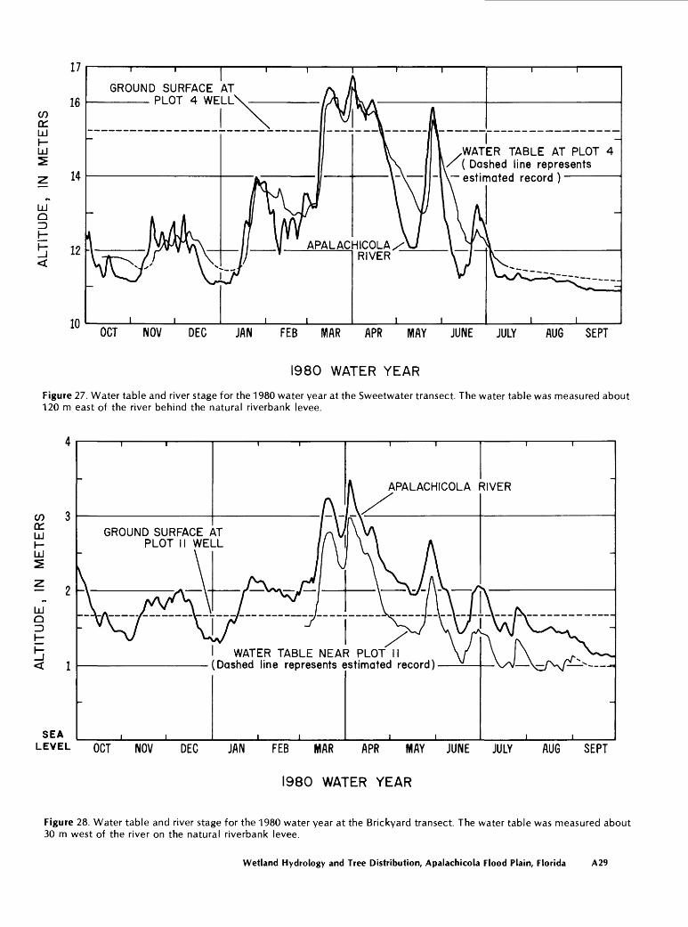
COcrUJh-UJ

UJ Q=)

GROUND SURFACE AT PLOT 4 WELL

.WATER TABLE AT PLOT 4 / ( Dashed line represents

estimated record )

APALACHICQLA^ RIVER


I960 WATER YEAR

Figure 27. Water table and river stage for the 1980 water year at the Sweetwater transect. The water table was measured about 120 m east of the river behind the natural riverbank levee.

co 3 crUJh-UJ

UJ Q=)

< 1

APALACHICOLA RIVER

GROUND SURFACE AT PLOT II WELL

I WATER TABLE NEAR PLOT (Dashed line represents estimated record)

SEA LEVEL OCT NOV DEC JAN FEB MAR APR MAY JUNE JULY AUG SEPT

1980 WATER YEAR

Figure 28. Water table and river stage for the 1980 water year at the Brickyard transect. The water table was measured about 30 m west of the river on the natural riverbank levee.


adjacent upland is continuous. At Brickyard, the water- table gradient is generally away from the river at low and medium stages and essentially the same as the river at high stages, depending upon the rate of rise or fall of river stage. The gradient at Brickyard may be towards the river at extremely low stages, but this condition did not occur during the period of investigation.

Trees

Species Composition

The cruise transects were designed to provide an estimate of the species composition of the whole flood plain. Results from point sampling methods on the in tensive transects gave mean basal areas and densities (of all species) that were roughly 10 percent smaller than plot sampling values. Others have compared plot and point sampling and found insignificant differences in the results of the two methods (Grosenbaugh and Stover, 1957). Further data, such as more sampling transects or a forest map, would be needed to test or im prove on this estimate of flood-plain composition.

Forty-seven species of trees were identified and measured during the study. Table 8 lists the 25 most

significant species ranked by basal area. Water tupelo is the most common tree in the flood plain in both basal area and density. Six wet-site species (water tupelo, Ogeechee tupelo, baldcypress, Carolina ash, swamp tupelo, and planertree) dominate the flood plain with a combined relative basal area of 64.8 percent. Their com bined relative density is 47.8 percent. Of the remaining 39 species, sweetgum stands out with 4.8 percent of the basal area and possumhaw (a deciduous holly) with 10.5 percent of the density.

Several species were notable with regard to their range of distribution. Swamp tupelo was observed only in the two lower river transects with a few minor excep tions. Sweetbay, cabbage palmetto, and pumpkin ash were found exclusively in the lower river. Ogeechee tupelo was relatively uncommon in the upper river. Sugarberry, possumhaw, and American hornbeam were rare or absent in the lower river. Sweetgum was found most commonly on the higher flats and terraces of the upper and middle river, but could also be found occa sionally in permanently saturated soils of the lower river. The upper river had the greatest variety of species, probably because of the greater range in elevations and hydrologic fluctuations. Of 47 species sampled, 35 were found in the upper river, and 27 were found in the lower river.

Table 8. Relative importance of tree species on the Apalachicola River flood plain based on cruise-transect data[Absolute basal area and density upon which these percentages are based are 46.2 mVha (square meters per hectare) and 1,540 trees/ha (trees per

hectare), respectively. Due to Founding, percentages given will not necessarily total 100]

Species

Water tupeloOgeechee tupeloBaldcypressCarolina ashSwamp tupeloSweetgumOvercup oakPlanertreeGreen ashWater hickorySugarberryDiamond-leaf oak _American elm

Relative basal area, in percent

29.911.010.65.45.04.83.22.92.92.92.82.52.4

Relative density, in

percent

12.86.65.5

11.52.03.22.09.42.7

.82.11.41.2

Species

American hornbeamPumpkin ash 1Water oakRed mapleSweetbayRiver birchPossumhawAmerican sycamoreSwamp cottonwood _Black willowSwamp chestnut oakBox elder22 other species2

Relative basal area, in percent

2.01.91.81.51.0

.8

.8

.6

.4

.4

.3

.32.0

Relative density, in

percent

4.74.4

.54.8

.5

.710.5

.3

.4

.4

.1

.810.7

'Some trees identified as pumpkin ash may have been Carolina ash or green ash. Samaras (winged seeds) had dropped from the trees and seeds of all three species were mixed on the ground beneath the trees.

2Green haw, cabbage palmetto, water locust, red mulberry, swamp-privet, winged elm, slippery elm, cherrybark oak, stiffcornel dogwood, chinaberry, black tupelo, buttonbush, spruce pine, loblolly pine, laurel oak, buckthorn bumelia, parsley haw, common persimmon, black walnut, titi, withered viburnum, and little silverbell. Grape vines were also counted at several sampling points.


Forest Types

Five forest types were defined using the cruise- transect data (table 9); examples of three of the types, A, B, and E, are shown in figure 29. Relative basal areas and densities of tree species in each forest type are given in tables 10 and 11. An attempt was made to identify each cruise-transect point as one of the five types. Four teen of the 223 points, however, could not be classified because they did not meet any of the forest type defini tions in table 9. Unclassified points had species com positions intermediate between two or three forest types, had dominant pioneer or early successional species, or had no trees.

D and E could be considered the same forest type, but the conspicuous presence of swamp tupelo in the lower river suggested a division between the two types. Swamp tupelo sites are characterized by shallower flooding according to Eyre (1980, p. 69).

One forest type on the Apalachicola River not sampled by the cruise transects is Society of American Foresters type 95 (Eyre, 1980). In this type, black willow is usually pure or predominant, and swamp cottonwood, river birch, and American sycamore are chief associates. This is a pioneer type characteristically found on the new land formed by point bars. Although it is very common along the river margins, usually on the inside of each bend in the river, this willow zone is

Table 9. Forest types defined at the cruise transects [Predominant: comprising 50 percent or more of basal area; Pure: comprising 95 percent or more of basal area]

Name Definition Chief associates Common associates SAP 1 type

Type A:Sweetgum-sugar-

berry-water oak.

Type B:Water hickory-green

ash-overcup oakdiamond-leaf oak.

Type C:Water tupelo-

Ogeechee tupelobaldcypress.

Type D:Water tupelo-swamp

tupelo.

TypeE:Water tupelo-bald-

cypress

Sweetgum, sugarberry, water oak, American hornbeam, possumhaw are predom inant.

Water hickory, green ash, overcup oak, dia mond-leaf oak, sweetgum, American elm are predominant.

Water tupelo, Ogeechee tupelo, baldcypress, swamp tupelo, Caro lina ash, planertree are predominant but not pure.

Water tupelo, swamp tupelo, Ogeechee tupelo, baldcypress, Carolina ash, pump kin ash, planertree, sweetbay are pure. 2

Water tupelo, baldcypress, Ogeechee tupelo, Carolina ash, planertree are pure.

Diamond-leaf oak, green ash.

Sugarberry, red maple _

Overcup oak, pumpkin ash, red maple.

American elm, American sycamore, water hick ory.

Water oak, possumhaw, American hornbeam, water tupelo, Ogee chee tupelo, baldcypress.

Water hickory, Ameri can elm, green ash, diamond-leaf oak, sweetbay.

92

93 or 96

102 or 103

103

102 or 103

'Society of American Foresters (Eyre, 1980).2Swamp tupelo, pumpkin ash, or sweetbay serve as indicator species to distinguish this type from type E.


Table 10. Relative basal areas of tree species of each forest type, derived from cruise-transect data

[Absolute basal areas upon which these percentages are based are 28.5 mVha for forest type A, 32.8 mVha for B, 53.6 mVha for C, 66.1 m 2/ha for D, and 59.2 m 2/ha for E. Due to rounding, percentages given will not necessarily total 100. Species from 14 of the 223 cruise-transect points are not included because those points could not be classified into any of the five types defined in table 9]

SpeciesRelative basal area (in percent)

Type

A

Type B

Type C

Type D

Type E

Table 11. Relative densities of tree species of each forest type, derived from cruise-transect data[Absolute densities upon which these percentages are based are 1,340 trees/ha for forest type A; 1,360 trees/ha for B; 2,210 trees/ha for C; 2,050 trees/ha for D; and 1,120 trees/ha for E. Densities of some of the understory species may appear relatively high because no minimum diameter limit was used during sampling. Due to rounding, percentages given will not necessarily total 100. Species from 14 of the 223 cruise-transect points are not included because those points could not be classified into any of the five types de fined in table 9]

Loblolly pine _____ 0.2Spruce pine _____ .4Cherrybark oak ___ .4Chinaberry _____ .2Buckthorn bumelia _ .2Parsley haw _____ .2Red mulberry ____ .9Winged elm _____ .8Black tupelo _____ .4Boxelder _______ .9Swamp chestnut oak _ 1.8Possumhaw _____ 4.8Water oak ______ 11.7Sugarberry ______ 16.7Sweetgum ______ 25.9American hornbeam __ 12.0American sycamore _ 2.7

0.3 ___..5 ___..5 ___.

1.3 ____.1.4 ____.3.3 ____.9.8 0.52.4 .31.2 .1

Swamp-privet ____ 1.1 ___ .1 _____________Green haw ______ .4 .8 ______________Green ash _______ 4.3 15.8 1.9 _____________American elm ____ 3.6 11.4 1.7 _____________Water hickory ____ 2.4 15.8 1.3 _____________Stiff cornel dogwood _____ .3 ______________Laurel oak ___________ .3 _ _____________Diamond-leaf oak __ 3.8 10.9 2.2 _____________Overcup oak _____ 1.1 14.7 4.8 _________Red maple ______ 1.1 2.8 3.7 _____________Water locust _____ .2 .3 .4 _____________Cabbage palmetto __ .4 ___ .7 _____________River birch _______________ 1.2 _________Slippery elm ______________ .2 ___________Black willow ______________ .9 ___________Swamp cottonwood __________ .7 _________Pumpkin ash1 _____________ 4.4 5.4 .Sweetbay________________ 2.1 3.2 _ .Swamp tupelo ____ .4 .3 6.8 20.0 .Buttonbush_______________ .2 ___ 0.1Planertree ___________ .4 6.6 3.0 2.3Carolina ash _____ .2 1.7 9.8 2.1 7.1Ogeechee tupelo _______ 1.3 14.2 20.7 12.4Water tupelo _____ .2 .9 24.8 34.5 58.4Baldcypress _____ .2 1.0 10.2 11.0 19.8

'Some trees identified as pumpkin ash may have been Carolina or green ash. Samaras (winged seeds) had dropped from the trees and seeds of all three species were mixed on the ground beneath the trees.

Relative density (in percent)Species

Loblolly pineSpruce pineCherrybark oakChinaberryBuckthorn bumeliaParsley hawRed mulberryWinged elmBlack tupeloBoxelderSwamp chestnut oakPossumhawWater oakSugarberrySweetgumAmerican hornbeam _ American sycamoreSwamp-privetGreen hawGreen ashAmerican elmWater hickoryStiff cornel dogwoodLaurel oakDiamond-leaf oakOvercup oakRed mapleWater locustCabbage palmettoRiver birchSlippery elmBlack willowSwamp cottonwoodPumpkin ash 1SweetbaySwamp tupeloButtonbushPlanertreeCarolina ashOgeechee tupeloWater tupeloBaldcypress

Type A

<0.1<.l<.l

.3

.2 3.8

.3

.3<.l 2.9

.3 37.8 2.3 7.9 8.1

22.0 1.1 4 1

.5

.6

.9

.7

3.2 .8 .9 .1 .1 .

.2

.1

<.l<.l

Type B

0.1 .3

<.l 25.1

.3 3.6 9.3 2.7

.3

.7 11.5 4.7 3.7 4.9

<0.12.3 8.1

16.9 .1

.7

<.l

.1 1.9

.1

.6 1.8

Type Type C D

0.8.3

<.l.3

3.31.1

.3

1.42.46.91.8

.3

.9

.21.1

.5. 4.5 21.4.. 1.1 1.2.

2.7 8.2 7.7

17.6 22.0 18.2 11.5 10.1 6.8 10.3 24.2 5.9 4.5

Type E

0.3 6.8

25.0 15.6 35.6 16.6

'Some trees identified as pumpkin ash may have been Carolina or green ash. Samaras (winged seeds) had dropped from the trees and seeds of all three species were mixed on the ground beneath the trees.


Type B, near kilometer 127, showing silt deposition on tree trunks about 2 m above ground (at arrow).

Type A, near kilometer 158, showing large sweetgums surrounded by abundant vines and undergrowth.

Type E, near kilometer 37, with water tupelo predominant.

Type E, near kilometer 20, with baldcypress in foreground.

Figure 29. Forest types A, B, and E.

quite narrow and occupies a very small part of the total area of the flood-plain forest.

A very common Mississippi River flood-plain community type, overcup oak-water hickory, was occa sionally found in limited areas. Results of sampling did not indicate that it was consistent or extensive enough to be categorized as a separate forest type.

The most common single forest type is E (table 12). The three forest types dominated by tupelo and other wet-site species, C, D, and E, constitute a total of 56 percent of all sample points. The change in abun dance of different forest types from upper to lower river is shown in figure 30. Type A decreases downstream and type B, well represented in the upper and middle river, is almost completely absent in the lower river. Type C is concentrated at the three downstream transects. Type D occurs almost exclusively at the two lower river transects. Type E is the only type present at all eight transects.

Mean basal areas in rnVha of all tree species are below average at sites identified as types A and B, and above average at sites belonging to types C, D, and E (fig. 31). Mean densities in trees/ha show a similar trend except for type E. Some of this difference in basal area and density may be due to the enlarged bases of tupelo and cypress trees that dominate types C, D, and E, although tree trunks were sampled above the swelled buttresses whenever possible. This higher basal area and density of types C, D, and E, in combination with a downstream increase in abundance of the three types (fig. 30), explains the downstream increase in basal area and density shown in figure 32.

Water and Tree Relations

The Kruskal-Wallis test (Hollander and Wolfe, 1973, p. 117) was used to test differences among forest types with respect to the nine water parameters. For each water parameter, values were assigned rankings and an analysis of variance was performed on the rank ed values rather than the actual values. The F-value (model mean square/error mean square) was tested for significance at a 0.0001 level of significance. With respect to eight of the nine water parameters, dif ferences existed among forest types at a significance probability of 0.0001. The only parameter that did not show this relation to forest types was velocity. At a significance probability of 0.01, however, it was also shown to vary among forest types. River location was tested in addition to the nine water parameters and showed differences among forest types at a significance probability of 0.0001.

Some of the water parameters were derived direct ly from others or from the same basic data. Correlation coefficients of each of the nine water parameters with each other and river location were calculated to deter mine the degree of interdependency among parameters (table 13). Correlation coefficients and significance probabilities were calculated by the Pearson product- moment method. The six parameters measuring dura tion of inundation and saturation all have highly signifi cant correlations with each other. Kilometers, fall- season depths, and flood depths are strongly correlated with most of the duration parameters. Velocities have the weakest correlations with the other parameters.

Table 12. Abundance of forest types at all cruise transects

Forest typeNumber of

sample points

Percent of totalsample points

(rounded)

A ________. B _______. C _______. D ______.E _______.Unclassified _.

Total ___

473647255414

223

2116211124

6

Each of the nine water parameters was compared to the five forest types at all sites (209 cruise-transect points). The combining of all sites in making a com parison, however, frequently masks patterns of water and tree relations that change from upper to lower river. To illustrate how relations change at different locations on the river, most parameters are presented not only for all sites but are also presented for 53 cruise-transect points in the upper river and for 81 points in the lower river. The remaining points in the middle river are not shown separately because conditions there are generally between those of the two extreme locations in the upper and lower river. Upper river graphs compare only A, B, and E forest types because C and D types are rare in the upper river. Lower river graphs show only C, D, and E types because A and B types are rare in the lower river (see fig. 30).


100

CO

171 160 140 120 100 80 60 40 20

DISTANCE ABOVE MOUTH OF RIVER, IN KILOMETERS

EX PLANATION

FOREST TYPES CRUISE TRANSECT NAMES

0

A

B

C

D E

Unclassified

KM 169 - ChattahoocheeKM 150 - Torreya ParkKM 138 - SweetwaterKM 117 -Old RiverKM 98 - Muscogee ReachKM 79 - Porter LakeKM 32 - BrickyardKM 20 - South end of Forbes Island

Figure 30. Abundance of forest types at each cruise transect.


UJ (E Ul^ Q-3 £ ot-(0

UJ

..a: < uUJ CL (T«8

< I- V) uCD 2

3U

onou

70

60

50

40

30

20

10

n

EXPLANATION|x| Mean basal area for[±J forest type shown. ~

0 Mean density for foresttype shown.

Mean basal area and densityfor all fores!

~

__ _ _ _ _

_ £

* 1 n

:

xI ; :

type

sm

V

£1

^

?!

£

:|:

x

^

\-

-

ouuu

2750Ul

2500 <r<

2250 oT~

2000 Q,

1750 "V)

1500 ui

1250 H

1000 >-i-

750 wUJ

500 a

250

nB

FOREST TYPESFigure 31. Mean basal area and density of trees of each forest type.

Depth of Water

Fall-Season Depth

Figure 33 shows the 1979 fall-season depths for each forest type. Types A and B were generally dry. Types C, D, and E were generally wet, although the range of C overlapped that of A and B.

Upper river types fell into two very distinct cate gories: dry (A and B), and saturated or inundated (E). Lower river types were generally inundated with 0.1 m of water and showed little difference in median depths; however, type C was much more variable than D and E, ranging from dry to 0.6 m deep in the fall.

UJ

130

120

a no

±. V)

UJ»-

100

90

UJ<r< 70o <" 60

40

3 30CD

10

0

EXPLANATION

Mean basal area for each cruise transect.

o o Mean density foreach cruise transect.

Mean basal area and density for all cruise transects.

CRUISE TRANSECT NAMES

Km 169 ChattahaocheeKm 150 Torreya Park

.Km !38--SweetwaterKm 117 Old RiverKm 98--Muscogee ReachKm 79 Porter Lake

'Km 32 BrickyardKm 20 South end of Forbes Island

UJ

UJ

enUJ

V)

4750

4500

4250

4000

3750

3500

3250

3000

2750

2500UJac

2250 H

2000 \

1750 tV)

1500 g

1250

1000

750

500

250

'171 150 125 100 75 50 25 0 DISTANCE ABOVE MOUTH OF

RIVER, IN KILOMETERSFigure 32. Mean basal area and density of trees at each cruise transect.

Flood Depth

Flood depth is a relative measure of elevation cor rected to a standard reference the 2-year, 1-day high. This parameter allows relative elevational comparisons among forest types at transects which differ greatly in land-surface altitude. Altitude; 2-year, 1-day high; and forest type of each cruise-transect point are shown on cross sections in figure 34. Large elevation differences between forest types are characteristic of the upper river. The lower river flood plain is very flat with little or no elevation difference between forest types. This

geographic difference can be explained by the decrease in water fluctuation from upper to lower river. Higher flood stages create higher levees in the upper river than in the lower river. Upper river levees are 3 to 6 m higher than low and medium river stages, whereas lower river levees are 0.6 to 1.8 m higher than those same river stages. Although duration of flooding may be equal for levees at the two locations, more xeric (drier) species will be able to grow on the upper river levee due to the distance from the water table. Thus the greater range in


Table 13. Significant correlation coefficients of nine water parameters with each other and river location [Levels of significance are: 0.0001 for correlation coefficients of 0.26 to 0.99; 0.001 for correlation coefficients of 0.22 to 0.25; and 0.01 for cor

relation coefficients of 0.17 to 0.21. NS = not significant]

Consecutive days ofsaturation

Observed percent inundationObserved consecutive days of

inundationFall-season depthPercent inundation estimated

from river stageConsecutive days of inunda

tion estimated from riverstage

KilometersFlood depthVelocity

Percentsaturation

0.99.85

.73

.86

.62

.50-.49-.45

NS

Consecutivedays of

saturation

0.82 .

.72

.84

.56

.44-.45

.40NS

Observedpercent

inundation

0.96.85

.50

.40-.27

.59NS

Observedconsecutive

days ofinundation

0.79

.29

.21NS.60NS

Fall-seasondepth

0.57

.50-.36

.49NS

Percentinundationestimatedfrom river

stage

0.97.78.20.23

Consecutive days of

inundationestimatedfrom river

stage Kilometers Flood depth

0.70NS 0.29.18 .37 NS

ALL SITES UPPER RIVER ONLY LOWER RIVER ONLY

Dry

DampUJ O

2 5 Satur-~.o ate<Ji"o

t-lo§

gi -°-5

-1.0

I I

O T

<? 6 0

B E C

FOREST TYPES

EXPLANATIONDiagram explaining vertical axis:

Dry

Median and range for forest type indicated

Ground surface-I.Om

Figure 33. Relations between 1979 fall-season water depth and forest type.


CHATTAHOOCHEE (KM 169)

TORREYA PARK (KM 150)

EXPLANATION2-YEAR, 1-DAY HIGH (1958-80). CRUISE-TRANSECT POINTS. Letters represent forest type (U=unclassified). SAMPLE PLOTS. Numerals represent plots along the Sweetwater and Brickyard intensive transects. MEASURED ALTITUDE. APPROXIMATE ALTITUDE estimated from topographic maps.

14

SWEETWATER (KM 138)

10

OLD RIVER (KM 117)

500I_

1000 METERS _I

Figure 34. Altitude; 2-year, 1-day high (1958-80); and forest type for each cruise-transect point.


MUSCOGEE REACH (KM 98)

PORTER LAKE (KM 79)10

4-

cc uj

., SEast West

BRICKYARD (KM 32)

4

2

SEALEVEL

2

4

SOUTH END OF FORBES ISLAND (KM 20)

<

-I

-

CE[ COC[

\_ - - ' i i/

v-~_ . Humphreys East River S(oHughy

-East

. C(D

£(O

oo.c o(O

(On

A

UsV

Little Brothers Slough /""

D

y

OCECOCcOCOCCCCDO[ CC OOCOOOooO[

,_ "(D

bew _0) i

11 West""

500 1000 METERSI______I

Figure 34. Continued.


water fluctuation in the upper river creates larger elevational differences allowing wider variations' in forest types than in the lower river.

Figure 35 shows flood depths for each forest type. When all sites are considered together, median flood depths for all forest types are between 1.2 and 2.7 m, and ranges show much overlap. However, considering only the upper river, the flood depths in type E forests were much greater, ranging from 2.7 to 4.6 m deep, than in type A and B forests. In the lower river, flood depths are shallower and less variable than in the upper river. Median flood depths for all lower river forest types were between 1.2 and 2.1 m, and total range of flood depths was less than one-third of that in the upper river.

Elevational differences among forest types in the lower river are of greater importance than implied by the results shown in figure 35 because ground levels were measured in such a way that microrelief was not taken into account. Microrelief in the hummocky land between Brickyard Cutoff and Brothers River is prob ably the primary factor influencing tree growth there. Hummocks only a few meters in diameter rise above the average level of the flood plain allowing tree roots to obtain plenty of oxygen in a permanently inundated en vironment.

Flood depths for one forest type, E, are shown in figure 36 at every transect. Depths gradually and con sistently decrease from upper to lower river.

ALL SITES UPPER RIVER ONLY LOWER RIVER ONLY

to

IIm 2

o -

5s -,OQ I

UJ <U O o

K

*° < .gui -C

-4

5

<>

ABE

FOREST TYPE

EXPLANATIONDiagram explaining vertical axis

Median and range for forest type indicated ^Water surface

2-year, 1-day high

Ground surface

Figure 35. Relations between 2-year, 1-day high (1958-80) flood depth and forest type.


CO(rUJ»-UJ -2

" 3

o - -4

-5171 150 100 50 0

DISTANCE ABOVE MOUTH OF RIVER, IN KILOMETERS

EXPLANATION TRANSECT NAMES

Km 169-ChattahoocheeKm 150-Torreya ParkKm 138- SweetwaterKm 117-Old RiverKm 98 - Muscogee ReachKm 79-Porter LakeKm 32-BrickyardKm 20 - South end of Forbes Island

Figure 36. Two-year, 1-day high (1958-80) flood depths at type E forests at each transect.

Duration of Inundation and Saturation

Supplementary Data II (p. A49) summarizes the hydrologic observations and assumptions at each transect that were used to estimate values for four of the six duration parameters, observed percentage of inun dation, percentage of saturation, observed consecutive days of inundation, and consecutive days of saturation.

The nine numbered graphs in figure 37 show various estimates of percentage of inundation and saturation for each forest type. Figure 38 shows estimates of consecutive days of inundation and satura tion in the growing season for each forest type in the same format as figure 37. In the following paragraphs, references to individual graphs apply to both figures.

For types A and B, median time of inundation estimated from river-stage record (graph 1), observed time of inundation (graph 4), and estimated time of saturation (graph 7), are similar. Types A and B were generally found on levees, ridges, slopes, or high flats with hydrologic fluctuations that matched river stage. Time of inundation estimated from river-stage record was determined to be a good measure of the actual inun dation and saturation conditions in the flood plain for those forest types. (See figure 34 and Supplementary Data II for details at each transect.)

Graphs 1, 4, and 7 show that for types C, D, and E, time of inundation estimated from river-stage record is much less reliable as a measure of actual inundation conditions in the flood plain and is almost completely useless an an indicator of actual saturation conditions in the flood plain. Types C, D, and E were commonly found in low, permanently saturated flat areas with poor drainage connections to the river.

Graphs 5 and 8 show that forest types in the upper river fall into two very distinct hydrologic groups. Me dian time of inundation and saturation is less than 20 percent (fig. 37) or 25 consecutive days in the growing season (fig. 38) for types A and B and 100 percent or 266 days (the entire growing season) for type E. Graphs 6 and 9 show that hydrologic distinctions between forest types in the lower river are much less clear than in the upper river. Median time of inundation and saturation in the lower river is less for type C but still greater than 50 percent or 80 consecutive days in the growing season for all three forest types.

In general, types C, D, and E are commonly found on permanently saturated soil, whereas types A and B are not. When the differences in basal area and density among forest types (fig. 31) are considered, it appears that biomass is greater in forests growing on permanently saturated soils. A possible explanation is that drier sites have been subjected to more frequent logging because of easier access, so that trees there are younger and of lower biomass. In the absence of any detailed history of logging practices, however, this ex planation cannot be confirmed.

In a comparison of estimated time of saturation with individual species, sweetgum and sugarberry were present most often at cruise-transect points saturated 10 to 15 percent of the time (about 3 consecutive weeks in the growing season). The median time of saturation was 22 percent (5 consecutive weeks in the growing season) for green ash, diamond-leaf oak, and water hickory, and 42 percent (more than 8 consecutive weeks in the growing season) for overcup oak. Baldcypress, water tupelo, Ogeechee tupelo, Carolina ash, swamp tupelo, and planertree occurred most often at points saturated


ALL SITES

BOD

UPPER RIVER ONLY ABE

LOWER RIVER ONLY

C D E

100si £ 80 o5 aUJ ~-

* uj 60o «

£ K 40=1 UJ

S i 20ss =s o

100

S 80

<« S§ 60ae ae

is 40UJ

£ 20

0

100

z 80

^ S 60

S 40UJ CJoe£ 20

0

-

_

_

T c

ft 4

(

> J

» «

) ^

>

)

\::V_ JL

O-

-

-<

- T 0 J

» « [ JC

::.

Oq

"

-

p <j) C

»

)

TO*

T

I

T I §T

2

(:

I 6$

I

)

00

i Y

I I L^^J7

i i r0

1 . :.

O-

1 f I : "

O

i T I:..

-

-

Ci^yBODE

ALL SITES

ABE

UPPER RIVER ONLY

C D E

LOWER RIVER ONLY

EXPLANATION

I MEDIAN AND RANGE FORT FOREST TYPES INDICATED

LETTERS ON HORIZONTAL AXIS REPRESENT FOREST TYPES.

Figure 37. Relations between percentage of inundation and saturation (1958-80) and forest type.


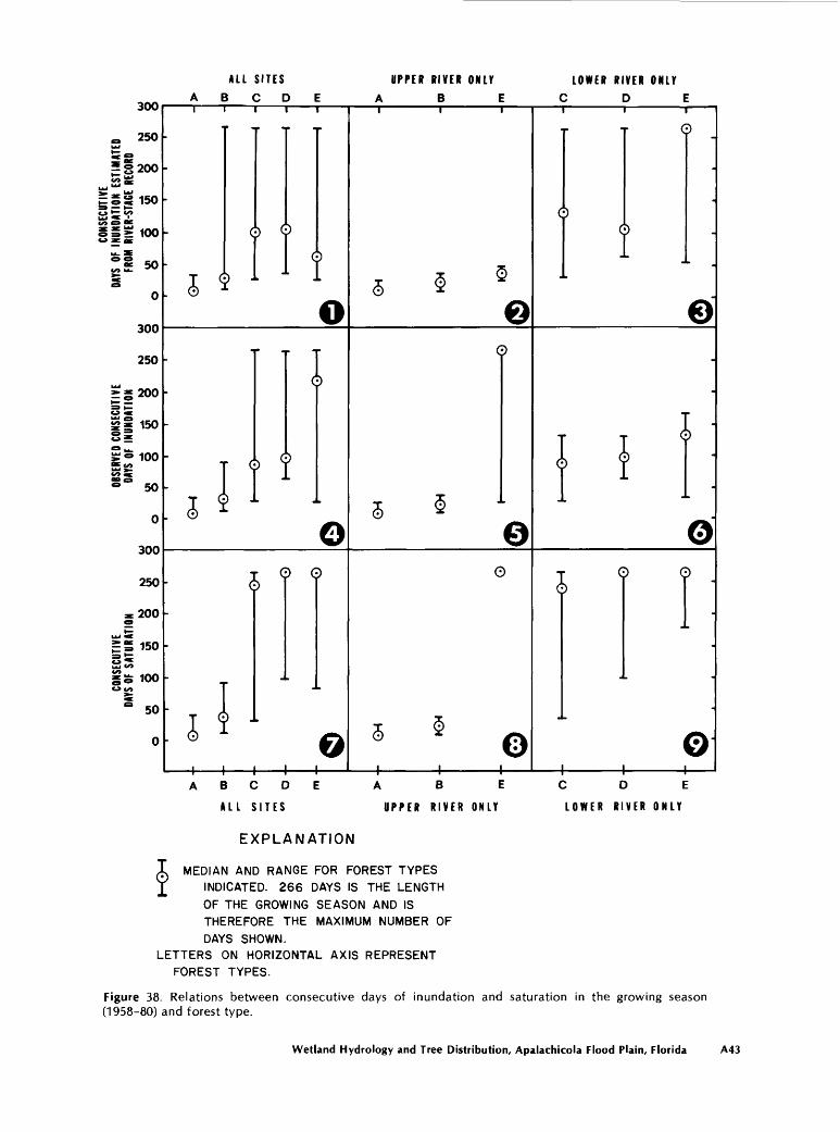
ALL SITES

A B C D E

UPPER RIVER ONLY

ABE

LOWER RIVER ONLY

C D E

B C D E

ALL SITES

EXPLANATION

ABE

UPPER RIVER ONLY

JUU

a 250UJN- o

(/> ac UJ 1*1

HI 150

siii = » 100t» SB ae

u. S

*£ 50

s0

250

OBSERVED CONSECUTI VI DAYS OF INUNDATION

D S 1 S I

250

z 200o t

UJ ^

= S 150CJ ^LJU <^

i= 100

2 50

0

1

i e ^

: j ^

: J i i

III

» « » «

o 0 1[in :o

i:

-

:'

' T

:o

; r Cp cj>

1 o

1 1

5 3 B

C

5 8 J

)p

0©

5 8L,,,.,, ,J ,. 11

1 1 1

(

»

)

c

I j

-

L

©

I'l ;

\»J

I ( j> C5

..

0C D E

LOWER RIVER ONLY

I MEDIAN AND RANGE FOR FOREST TYPES ][ INDICATED. 266 DAYS IS THE LENGTH

OF THE GROWING SEASON AND ISTHEREFORE THE MAXIMUM NUMBER OF

DAYS SHOWN.LETTERS ON HORIZONTAL AXIS REPRESENT

FOREST TYPES.

Figure 38. Relations between consecutive days of inundation and saturation in the growing season (1958-80) and forest type.


100 percent of the time. Table 14 compares relative tolerance to inundation and saturation of the 12 major species in this investigation to that of the same species in various field and greenhouse studies in the eastern United States.

Velocity

Average velocities in the flood plain during the 2-year, 1-day high (1958-80) range from 0 to 0.27 m/s (fig. 39). Most sites, regardless of forest type, have velocities between 0.1 and 0.2 m/s, and ranges for each forest type show much overlap. Most sites in the upper river, regardless of forest type, have velocities less than 0.06 m/s. Middle and lower river velocities are higher, most of them falling between 0.1 and 0.2 m/s.

Velocities showed no obvious differences with respect to forest types except at one location. At the Brickyard transect, velocities were generally higher in type C forests than type E. Type C forests were found on the hummocky land between Brickyard Cutoff and the Brothers River. The hummocks may be a velocity feature or created by roots as an adaptation to perma nent inundation. Velocities at all other transects were so variable that it would be difficult to draw firm conclu sions from this isloated case.

SUMMARY

The first major objective of this investigation was to observe hydrologic conditions in the forested flood plain and relate them to long-term river-stage record.

Analysis of long-term record for the Apalachicola River at Chattahoochee indicated that the 1958-79 average annual and monthly flows and the flow dura tions were significantly greater than those of 1929-57. Higher flows for the later period at stations on several other southeastern rivers indicated that climatic changes were probably responsible for the increased flow. However, due to physical changes in the channel, stages for the later periods were lower at Chattahoochee and the same at Blountstown compared to those of the earlier period.

Observations of hydrologic conditions in the flood plain during the 1980 water year were ex trapolated to approximate long-term (1958-80) condi tions. Hydrologic relations between the river and flood plain varied with each location. Natural levees on river and streambanks and high ridges within the flood plain were inundated only when the river reached relatively high stages. Water drained away from these areas as soon as river stages fell. Low, flat areas in the flood plain were almost always saturated and at some loca tions in the upper river appeared to be permanently in undated. Flood-plain areas of intermediate elevation between levees and low flats were generally inundated

0.3

E 0.2

O.I

6o

i

A B C D

FOREST TYPE

EXPLANATION

MEDIAN AND RANGE FOR FOREST TYPES INDICATED

Figure 39. Relation between average velocities during the 2-year, 1-day high (1958-80) and forest type.

for longer durations than the levees but were rarely saturated for prolonged periods. Height of natural riverbank levees and size and distribution of breaks in the levees had a major controlling effect on hydrologic conditions in the flood plain at all locations. A flood- plain stream, Brothers River, 32 km upstream of the bay, was commonly under tidal influence during times of low flow in the 1980 water year. At the same distance upstream of the bay, the Apalachicola River was not under tidal influence during the 1980 water year.

The second objective of this report was to estimate species composition and define the major forest types of the flood plain.

Of the 47 species of trees sampled, the five most common were wet-site species constituting 62 percent of the total basal area. In order of abundance, they were water tupelo, Ogeechee tupelo, baldcypress, Carolina ash, and swamp tupelo. Other very common species were sweetgum, overcup oak, planertree, green ash, water hickory, sugarberry, and diamond-leaf oak. Average basal area and density for all forest areas sampled were 46.2 mVha and 1,540 trees/ha, respec tively.

Several species were notable with regard to their range of distribution. Swamp tupelo was observed only in the two lower river transects with a few minor excep tions. Sweetbay, cabbage palmetto, and pumpkin ash were found exclusively in the lower river. Ogeechee tupelo was relatively uncommon in the upper river. Sugarberry, possumhaw, and American hornbeam were


Table 14. Comparison of relative tolerance of the 12 major flood-plain tree species to inundation and saturation in this investi gation to that found under various field and greenhouse situations in the eastern United States

[Grouped species have equivalent tolerances]

Relative tolerance This investigation

Lower White River, Dewatering project on Summary of literature Seedlings in green- Arkansas (Bedinger, a Kentucky reservoir on lower Mississippi house study in south-

1971) (Hall and Smith, Valley (Whitlow and ern Illinois (Hosner 1955) Harris, 1979) and Boyce, 1962)

Sweetgum,sugar berry.

Diamond-leaf oak, water hickory, green ash.

Sweetgum, ash.

Sugarberry,overcup oak, water hickory.

Overcup oak

Baldcypress, Planertree,water tupelo, baldcypress.swamp tupelo,Ogeechee tupelo,Carolina ash,planertree.

Sugarberry,swamp tupelo.

Sweetgum

Water tupelo, ash.

Overcup oak

Planertree

Sugarberry, sweetgum.

Sweetgum.

Green ash,water Hickory, overcup Oak, water tupelo, baldcypress, planertree.

Sugarberry.

Water tupelo.

Green ash.

rare or absent in the lower river. Sweetgum was found most commonly on the higher flats and terraces of the upper and middle river, but could also be found occa sionally in permanently saturated soils of the lower river. The upper river had the greatest variety of species.

Five forest types were defined on the basis of species predominance by basal area. They were type A, sweetgum-sugarberry-water oak; type B, water hickory- green ash-overcup oak-diamond-leaf oak; type C, water tupelo-Ogeechee tupelo-baldcypress; type D, water tupelo-swamp tupelo; and type E, water tupelobaldcypress. Biomass increased downstream and was greatest with forest types C, D, and E.

The third objective was to relate long-term hydrologic conditions in the flood plain to tree distribu tion.

Depth of water, duration of inundation and saturation, and water-level fluctuation, but not water velocity, were highly correlated with forest types. Forest types C, D, and E were generally found at sites having permanent soil saturation with inundation by flood waters 50 to 90 percent of the time or 75 to 225 con secutive days of each growing season from 1958 to 1980. Forest types A and B were found at sites that were saturated or inundated 5 to 25 percent of the time or 5 to 40 consecutive days of each growing season from 1958 to 1980.

Water and tree relations varied with river location because range in water-level fluctuation and topographic relief in the flood plain diminished downstream. River stage in the upper river fluctuated an average of 7.3 m. Ground surface varied 4.6 m across the upper river flood plain. As a result, forest types in the upper river included a wide variety of species grow ing among many different hydrologic conditions. Low flats occupied by forest type E experienced prolonged inundation with 0.5 m or more of standing water or per manent soil saturation. Relatively infrequent flooding occurred on levees and high ridges occupied by forest type A. Intermediate hydrologic conditions existed for sites occupied by forest type B. Ground surface in the flood plain of the lower river was very flat, usually vary ing no more than 0.6 m across the entire width of the flood plain at any one location. The range of river-stage fluctuation in the lower river was about one-third that of the upper river. Narrow levees, covering 6 to 8 per cent of the flood-plain width, provided the greatest topographic relief in the lower river. These levees were as much as 2.4 m above the flood-plain floor. Interior flood-plain soils were permanently saturated, except on tree hummocks. With few exceptions, lower river forests were dominated by water tupelo, Ogeechee tupelo, baldcypress, Carolina ash, and swamp tupelo (forest types C, D, and E).


SELECTED REFERENCES

Avery, T. E., 1967, Forest measurements: New York, McGraw- Hill, 290 p.

Bedinger, M. S., 1971, Forest species as indicators of flooding in the lower White River Valley, Arkansas: U.S. Geological Survey Professional Paper 750-C, p. C248-C253.

Brice, J. C., 1980, Measurement of bank recession on the Apalachicola River: Unpublished data on file at U.S. Geological Survey, Water Resources Division, Western Region, Office of Regional Hydrologist, Menlo Park, California.

Buchanan, T. J., and Somers, W. P., 1969, Discharge meas urements at gaging stations: U.S. Geological Survey Techniques of Water-Resources Investigations, Book 3, Chapter A8, 65 p.

Clewell, A. F., 1971, The vegetation of the Apalachicola National Forest: an ecological perspective: Atlanta, U.S. Department of Agriculture, Forest Service, 158 p.

1977, Geobotany of the Apalachicola River region: Conference on the Apalachicola drainage system, Gainesville, Florida, April 1976, Proceedings, p. 6-15.

Clewell, A. F., and McAninch, Helen, 1977, Effeccts of a fill operation on tree vitality in the Apalachicola River floodplain, Florida: Conference on the Apalachicola drainage system, Gainesville, Florida, April 1976, Pro ceedings, p. 16-19.

Conner, W. H., and Day, J. W., 1976, Productivity and com position of a bald-cypress-water tupelo site and a bot tomland hardwood site in a Louisiana swamp: American Journal of Botany, v. 63, p. 1354-1364.

Corbett, Don, and others, 1943, Stream-gaging procedure a manual describing methods and practices of the Geological Survey: U.S. Geological Survey Water-Supply Paper 888, 245 p.

Cowardin, L. M., Carter, Virginia, Golet, F. C., and LaRoe, E. T., 1979, Classification of wetlands and deepwater habitats of the United States: U.S. Fish and Wildlife Serv ice, Biological Services Program, FWS/OBS-79/31, 103 p. plus appendixes and plates.

Eichholz, N. F., Bailey, D. B., and McGehee, A. V., 1979, An investigation of dredged material disposal sites on the lower Apalachicola River: Tallahassee, Fla., Florida Game and Freshwater Fish Commission, Office of Envi ronmental Services, 115 p.

Elder, J. F., and Cairns, D. J., 1981, Production and decom position of forest litter fall on the Apalachicola River flood plain, Florida: U.S. Geological Survey Water- Supply Paper 2196-B, 42 p.

Eyre, F. H., editor, 1980, Forest cover types of the United States and Canada: Washington, D.C., Society of American Foresters, 148 p.

Foose, D. W., 1980, Drainage areas of selected surface-watersites in Florida: U.S. Geological Survey Open-File Report80-957, 83 p.

Fowells, H. A., compiler, 1965, Silvics of forest trees of theU.S.: U.S. Department of Agriculture Handbook No.271,762 p.

Frevert, R. K., Schwab, G. O., Edminster, T. W., and Barnes, K. K., 1955, Soil and water conservation engineering: New York, John Wiley and Sons, 479 p.

Greeson, P. E., editor, 1978, River-quality assessments: American Water Resources Association Symposium, Tuc- son, 1977, Proceedings, 191 p.

Grosenbaugh, L. R., and Stover, W. S., 1957, Point-sampling compared with plot-sampling in southeast Texas: Forest Science, v. 3, p. 2-14.

Hall, T. F., and Smith, G. E., 1955, Effects of flooding on woody plants, West Sandy Dewatering Project, Kentucky Reservoir: Journal of Forestry, v. 53, p. 281-285.

Harkins, J. R., Shell, J. D., Carter, R. F., and Rumenik, R. P., 1981, A method of estimating average streamflow and headwater limits in U.S. Army Corps of Engineers Mobile District, Alabama and adjacent States: U.S. Geological Survey Water-Resources Investigation, Open- File Report 81-59.

Harper, R. M., 1910, Preliminary report on the peat deposits of Florida: Florida State Geological Survey, Third An nual Report, p. 234-237.

1911, The riverbank vegetation of the lower Apala chicola, and a new principal illustrated thereby: Torreya, v. 11, no. 11, p. 225-234.

-1914, Geography and vegetation of northern Florida:Florida State Geological Survey, Sixth Annual Report, p. 210-216.

Hollander, Myles, and Wolfe, D. A., 1973, Nonparametric statistical methods: New York, John Wiley and Sons, 503P-

Hook, D. D., Brown, C. L., and Wetmore, R. H., 1972,Aeration in trees: Botanical Gazette, v. 133, no. 4, p.443-454.

Hosner, J. F., 1960, Relative tolerance to complete inundationof fourteen bottomland tree species: Forest Science, v. 6,no. 3, p. 246-251.

Hosner, J. F., and Boyce, S. G., 1962, Tolerance to water saturated soil of various bottomland hardwoods: Forest Science, v. 8, no. 2, p. 180-186.

Hubbell, T. H., Laessle, A. M., and Dickinson, J. C., Jr., 1956, The Flint-Chattahoochee-Apalachicola region and its environments: Bulletin of Florida State Museum, Biological Sciences, v. 1, p. 1-72.

Kulow, D. L., 1965, Elementary point-sampling: Morgan- town, West Virginia University, Agriculture Experiment Station, Circular 116, 24 p.

Kurz, Herman, 1938, A physiographic study of the tree asso ciations of the Apalachicola River: Proceedings of Florida Academy of Sciences, v. 3, p. 78-90.

Kurz, Herman, and Godfrey, R. K., 1962, Trees of northern Florida: Gainesville, University of Florida Press, 311 p.

Leitman, H. M., 1978, Correlation of Apalachicola River flood-plain tree communities with water levels, elevation, and soils: Florida State University Master's Thesis, 57 p.

Little, E. L., Jr., 1978, Atlas of United States Trees, v. 5, Florida: Miscellaneous Publication No. 1361, U.S. Department of Agriculture, Forest Service, 256 maps.

1979, Checklist of United States trees (native and naturalized): Agriculture Handbook No. 541, U.S. Department of Agriculture, Forest Service, 375 p.


Livingston, R. J., and Joyce, E. A., Jr., editors, 1977, Proceedings of the conference on the Apalachicola drainage system: Florida Department of Natural Resources: Marine Research Laboratory, Research Publication no. 26, 177 p.

Mattraw, H. C., Jr., and Elder, J. F., 1980, Nutrient yield of the Apalachicola River flood plain, Florida: river-quality assessment plan: U.S. Geological Survey Water- Resources Investigation 80-51, 21 p.

McAlpine, R. G., 1961, Yellow-poplar seedlings intolerant to flooding: Journal of Forestry, v. 59, p. 566-568.

Mueller-Dombois, Dieter, and Ellenberg, Heinz, 1974, Aims and methods of vegetation ecology: New York, John Wiley, 547 p.

Puri, H. S., and Vernon, R. O., 1964, Summary of the geology of Florida and a guidebook to the classic ex posures, special publication no. 5, revised: Florida Geological Survey, Tallahassee, Florida, 312 p.

Putnam, J. A., Furnival, G. M., and McKnight, J. S., 1960, Management and inventory of southern hardwoods: U.S. Department of Agriculture, Forest Service, Agriculture Handbook no. 181, 102 p.

Radford, A. E., Ahles, H. E., and Bell, C. R., 1968, Manual of the vascular flora of the Carolinas: Chapel Hill, University of North Carolina Press, 1183 p.

Rosenau, J. C., and Milner, R. S., 1981, Potentiometric sur face of the Floridan aquifer in the Northwest Florida Water Management District, May 1980: U.S. Geological Survey Water-Resources Investigations, Open-File Report 81-205.

Searcy, J. K., 1959, Flow duration curves: U.S. Geological Survey Water-Supply Paper 1542-A, 33 p.

Shearman, J. O., 1976, Computer applications for step- backwater and flood way analyses: U.S. Geological Survey Open-File Report 76-499, 103 p.

Smoot, G. F., and Novak, C. E., 1969, Measurement of discharge by the moving-boat method: U.S. Geological Survey Techniques of Water-Resources Investigations, Book 3, Chapter All, 22 p.

Southeastern Forest Experiment Station, 1958, Annual report 1957: U.S. Department of Agriculture, Forest Service, Asheville, North Carolina, 75 p.

U.S. Army Corps of Engineers, Mobile District, 1978, Co ordination report on navigational improvement for Apalachicola River below Jim Woodruff Dam, Florida (alternative report): 230 p.

1979, Section 404 (b) evaluation Apalachicola and lower Chattahoochee Rivers (operation and main tenance): Mobile, Alabama, 494 p.

-1980, 1979 Project Maps: Mobile, Alabama, 154 maps.U.S. Department of Agriculture, Forest Service, 1969, A

forest atlas of the South: 27 p.U.S. Department of Commerce, 1973a, Monthly normals of

temperature, precipitation, and heating and cooling degree days 1941-70-Florida: Climatography of the U.S. No. 81 (Florida), National Oceanic and Atmospheric Ad ministration, Environmental Data Service, National Climatic Center, Asheville, North Carolina, 8 p.

1973b, Monthly normals of temperature, precipitation, and heating and cooling degree days 1941-70 Georgia: Climatography of the U.S. No. 81 (Georgia), National Oceanic and Atmospheric Administration, Environmen tal Data Service, National Climatic Center, Asheville, North Carolina, 8 p.

1979a, Climatological Data Florida: National Oceanic and Atmospheric Administration, Environmental Data and Information Service, National Climatic Center, Asheville, North Carolina, v. 83, no. 8-12, 14 p. each.

1979b, Climatological Data Georgia: National Oceanic and Atmospheric Administration, Environmental Data and Information Service, National Climatic Center, Asheville, North Carolina, v. 83, no. 1-12, 14 p. each. 1980, Climatological Data Florida: National Oceanicand Atmospheric Administration, Environmental Data and Information Service, National Climatic Center, Asheville, North Carolina, v. 84, no. 1-9, 14 p.

U.S. Geological Survey, 1970, The national atlas: 417 p. 1976, Water-resources data for Florida 1975, north

ern Florida: Water-Data Report FL75-1. 1977, Water-Resources Data for Georgia Water Year

1976: U.S. Geological Survey Water-Data Report GA-76-1, 411 p.

1977-80, Water-resources data for Florida northwest Florida: Annual reports as follows: 1976, Water-Data Report FL76-4; 1977, Water-Data Report FL77-4; 1978, Water-Data Report FL78-4; 1979, Water-Data Report FL79-4.

Surface-water supply of the U.S., Pt. 2, South Atlantic slope and eastern Gulf of Mexico basins: Annual reports as follows: 1929, Water-Supply Paper 682; 1930, Water- Supply Paper 697; 1931, Water-Supply Paper 712; 1932, Water-Supply Paper 727; 1933, Water-Supply Paper 742; 1934, Water-Supply Paper 757; 1935, Water-Supply Paper 782; 1936, Water-Supply Paper 802; 1937, Water- Supply Paper 822; 1938, Water-Supply Paper 852; 1939, Water-Supply Paper 872; 1940, Water-Supply Paper 892; 1941, Water-Supply Paper 922; 1942, Water-Supply Paper 952; 1943, Water-Supply Paper 972; 1944, Water- Supply Paper 1002; 1945, Water-Supply Paper 1032; 1946, Water-Supply Paper 1052; 1947, Water-Supply Paper 1082; 1948, Water-Supply Paper 1112; 1949, Water-Supply Paper 1142; 1950, Water-Supply Paper 1172.

Surface-water supply of the U.S., Pt. 2-B, South Altantic Slope and eastern Gulf of Mexico basins, Ogeechee River to Pearl River: Annual Reports as follows: 1951, Water-Supply Paper 1204; 1952, Water- Supply Paper 1234; 1953, Water-Supply Paper 1274; 1954, Water-Supply Paper 1334; 1955, Water-Supply Paper 1384; 1956, Water-Supply Paper 1434; 1957, Water-Supply Paper 1504; 1958, Water-Supply Paper 1554; 1959, Water-Supply Paper 1624; 1960, Water- Supply Paper 1704.

Surface-water supply of the U.S., Pt. 2, South Altantic slope and eastern Gulf of Mexico basins, v. 3, Basins from Apalachicola River to Pearl River: Reports as follows: 1961-65, Water-Supply Paper 1906; 1966-70, Water-Supply Paper 2106.


1972-75, Water-resources data for Florida, streams, northern and central Florida: Annual reports as follows: 1971, Water-Data Report FL71-1; 1972, Water-Data Report FL72-1; 1973, Water-Data Report FL73-1; 1974; Water-Data Report FL74-1.

U.S. Water Resources Council, 1977, Guidelines for deter mining flood flow frequency (revised): Bulletin no. 17A of Hydrology Committee, 162 p.

Velz, C. J., 1977, River-quality assessment a rational scientific basis for pollution control and water-quality management, in Greeson, P. E., ed., River-quality assessments proceedings of a symposium: American Water Resources Association, p. 3-10.

Vernon, R. O., 1942, Tributary valley lakes of western Florida: Journal of Geomorphology, v. 5, no. 4, p. 302-311.

Wharton, C. H., Odum, H. T., Ewel, K., Duever, M., Lugo, A., Boyt, R., Bartholomew, J., DeBellevue, E., Brown, S., Brown, M., and Duever, L., 1977, Forested wetlands of Florida their management and use: Gainesville, University of Florida, 348 p.

Whitlow, T. H., and Harris, R. W., 1979, Flood tolerance in plants: A state-of-the-art review: Department of En vironmental Horticulture, University of California, Davis, Environmental and water quality operational studies, Technical Report E-79-2, 161 p. plus appedixes and tables.

Yelenosky, George, 1964, Tolerance of trees to deficiencies of soil aeration: International Shade Tree Conference, 40th, Durham, North Carolina, 1964, Proceedings, p. 127-146.


SUPPLEMENTARY DATA I TRANSECT END POINTS

Transect Transect end points

Chattahoochee:east _____________ Flood-plain vegetation continued indefinitely up an upland creek swamp; no obvious eleva

tion changes.west _____________ Change to upland vegetation; rapid rise in elevation.

Torreya Park:east _____________ Change to upland vegetation, rapid rise in elevation.west _________ Loblolly pines joined flood-plain forest; no obvious elevation changes.

Sweetwater:east _____________ Change to upland vegetation, rapid rise in elevation.west _____________ Overgrown fields with no mature trees; no obvious elevation changes.

Old River:east _________ Change to upland vegetation, rapid rise in elevation.west _____________ Loblolly pines joined flood-plain forest; no obvious elevation changes.

Muscogee Reach:east _____________ Change to upland vegetation, rapid rise in elevation.west _____________ Overgrown fields with no mature trees; no obvious elevation changes.

Porter Lake:east _____________ Impassable due to recent timber cutting.west _____________ Change to upland vegetation; rapid rise in elevation.

Brickyard:east _____________ Change to upland vegetation; rapid rise in elevation.west _____________ High manmade levee.

South end, Forbes Island:

east _____________ Incomplete due to project time constraints.west _________..___ Change to upland vegetation; rapid rise in elevation.

SUPPLEMENTARY DATA II DESCRIPTION OF INUNDATION AND SATURATION CONDITIONS AT EACH TRANSECT

Numerous hydrologic observations and assump tions were used in estimating duration of inundation and saturation at each cruise-transect point. This infor mation is summarized here, from east to west across each transect. The two intensive transects are reported first because the detailed hydrologic data collected there were helpful in making estimates at the other six transects. Descriptions of hydrologic subsections can be easily followed by referring to the appropriate cross sec tion of each transect in figure 34.

In this supplement, the term "river-stage estimates" is used to represent the two water parameters, percentage of inundation estimated from river-stage record, and consecutive days of inundation estimated from river-stage record. The term "flood- plain estimates" is used to represent the four water parameters, observed percentage of inundation, percen tage of saturation, observed consecutive days of inunda tion, and consecutive days of saturation.

Sweetwater Transect

The first 1,250 m of the Sweetwater transect, which includes plots 1 and 2, were permanently inun dated to a minimum depth of 0.3 m over the entire area. Water levels were very stable except during the flood of March and April 1980, when rise and fall of flood-plain water levels matched river-stage fluctuations (fig. 23). The remainder of the transect, including the last 400 m on the east side and all of the west side excluding streams, was not inundated or saturated except during the March and April flood. Flood-plain estimates were the same as river-stage estimates in this subsection. Ground levels of all the cruise-transect points on the west side were well above average annual river stage.

Brickyard Transect

At the Brickyard transect, the levee on the west bank of the Apalachicola River is high and continuous enough to have a major controlling effect on the hydrology of the flood plain behind it. Ground levels for the entire length of the transect behind the riverbank levee fall well below the level of average annual river


stage. However, flood-plain water levels do not rise to match river stage until the river stage rises- above an altitude of approximately 2.1 m. Figure 24 shows 1980 water-level fluctuations of the Apalachicola River and the flood plain at plot 12 and Brothers River, that il lustrate the hydrologic conditions at this transect.

The first 1,890 m of the Brickyard transect is Forbes Island, bounded on both sides by natural levees. The levees are dry except when the river level is above an altitude of approximately 2.1 m. The very flat flood plain between the levees is flooded to shallow depths (less than 0.5 m) when the river stage rises above an altitude of about 1.5 m and is deeply flooded (1 m and more) when the river stage rises above an altitude of about 2.1m. There is little or no standing water at other times when the river is below an altitude of about 1.5m. However, 16 monthly observations during the fall seasons of 1979 and 1980 indicate that the soil is per manently saturated, regardless of the river stage or the time clasped since it was last flooded.

The middle part of the Brickyard transect is also an island (unnamed); but unlike Forbes Island, it is not flat or bounded by levees. Hummocks, mounds of land at the bases of clumps of trees, are as high as 1.2 m above surrounding land (fig. 12). Land between hum mocks is riddled with shallow sloughs 25 to 50 mm deep that never dry out. The network of sloughs around the hummocks is connected to the Brothers River and prob ably fluctuates daily from tidal influence at low river stage. At those times the hummocks are dry and crack ed, allowing tree roots to get plenty of oxygen despite standing water a few meters away in the shallow sloughs. The area is considered dry at those times for the flood-plain estimates. At medium stages (between altitudes of approximately 1.5 and 2.1 m in the river), water rises in the shallow sloughs, partially inundating the hummocks. At high stages (above an altitude of ap proximately 2.1 m in the river), water covers all of the flood plain to a depth of 1.2 m or more.

The first 250 m of the transect west of Brothers River is similar to the hummocky land just described. Hummocks gradually disappear to the west, and the last 640 m of the transect is very flat. Monthly observations indicate this last section is permanently saturated and is inundated only when the river stage is above an altitude of about 1.5 m.

Chattahoochee Transect

In the fall of 1979, soil on the east side of the Chattahoochee transect was firm and dry. Several small but steep-sided streams are connected directly to the river, breeching the natural riverbank levee nearby to both the north and south. Flood-plain estimates corres pond to river-stage estimates in this section. Behind the

natural riverbank levee on the west side, water was ponded almost 1 m deep in the fall of 1979. Aerial observations in the fall of 1980 indicated that it was still ponded. Sites on the west side that were inundated or saturated in the fall of 1979 are judged to be permanent ly inundated or saturated. Flood-plain estimates for dry sites that were above the level of the ponded water are the same as river-stage estimates.

Torreya Park Transect

The first 275 m of the Torreya Park transect were saturated in the fall of 1979 and probably remain per manently saturated due to ground-water seepage from steep adjacent bluffs. The remainder of the transect on the east and west sides was firm and dry in the fall and is probably flooded directly by river-stage fluctuations.

Old River Transect

At the Old River transect, standing water 25 to 50 mm deep covered the first 610 m in the fall of 1979, and permanent inundation is assumed. A low ridge separates this section from the remainder of the east side transect. West of the ridge, soils were noticeably firmer, and most sites were dry. Observations during the flood of March and April 1980 indicated that this section drains more quickly than the river, probably by way of a flood- plain slough (Outside Lake) to the south. Flood-plain estimates west of the ridge correspond to river-stage estimates.

On the west side of the Old River transect, three low areas approximately 460, 820, and 1,680 m west of the riverbank were inundated, saturated, or immediate ly adjacent to standing water in the fall of 1979. The numerous depressions, sloughs without downstream outlets, and ponded water observed in both the fall dry period and spring floods indicated strong similarities to a site 10.5 km upstream studied by Leitman (1978). In that study, flood waters were found to be retained by numerous depressions and sloughs in the interior of the flood plain several weeks after flood waters had reced ed. For low and medium elevation sites on the west side of the Old River transect, flood-plain estimates were greater than river-stage estimates. For high elevation sites throughout the transect, flood-plain estimates were the same as river-stage estimates.

Muscogee Reach Transect

In the fall of 1979, water was ponded 0.5 m deep on the first 210 m of the Muscogee Reach transect, and permanent inundation is assumed. For the remaining areas of this transect (east and west sides) that were dry in the fall, flood-plain estimates match river-stage estimates. Five low areas on the west side of the transect


were damp, but not saturated, in the fall. Flood-plain estimates are slightly greater than river-stage estimates at these sites.

Porter Lake Transect

The two sites on the east riverbank levee of the Porter Lake transect were firm and dry in the fall of 1979. Flood-plain estimates match river-stage estimates at those sites. In the first 460 m of the west side there is a depression with no outlet during low water. Soils were saturated at two sites within this depression during the fall. Flood-plain estimates are greater than river-stage estimates at those sites. The last 580 m of this transect lie west of a dividing ridge. Flood waters west of this ridge have a direct outlet to the river by way of Porter Lake. For all sites not inundated or saturated in the fall, flood-plain estimates match river-stage estimates. Per manent inundation or saturation were assumed at wet sites.

South End of Forbes Island Transect

At the south end of Forbes Island transect, obser vations began 520 m east of the Apalachicola River at Humphreys Slough, which is connected to the Apalachicola River to the north and the St. Marks River to the south. Flood-plain estimates for inundation match river-stage estimates in the section from Hum phreys Slough to the Apalachicola River. Observations in the fall of 1979 and 1980 indicate that saturation is permanent in this section, except for the two east riverbank levee sites. The high levee on the west bank of the Apalachicola was dry in the fall. All remaining sites were saturated in the fall. Since Brothers River levees are not present to impound flood waters on or hold flood waters out of the flood plain, flood-plain estimates for inundation correspond to river-stage estimates. Saturation, however, is permanent probably because the land is very flat and altitudes are close to sea level.


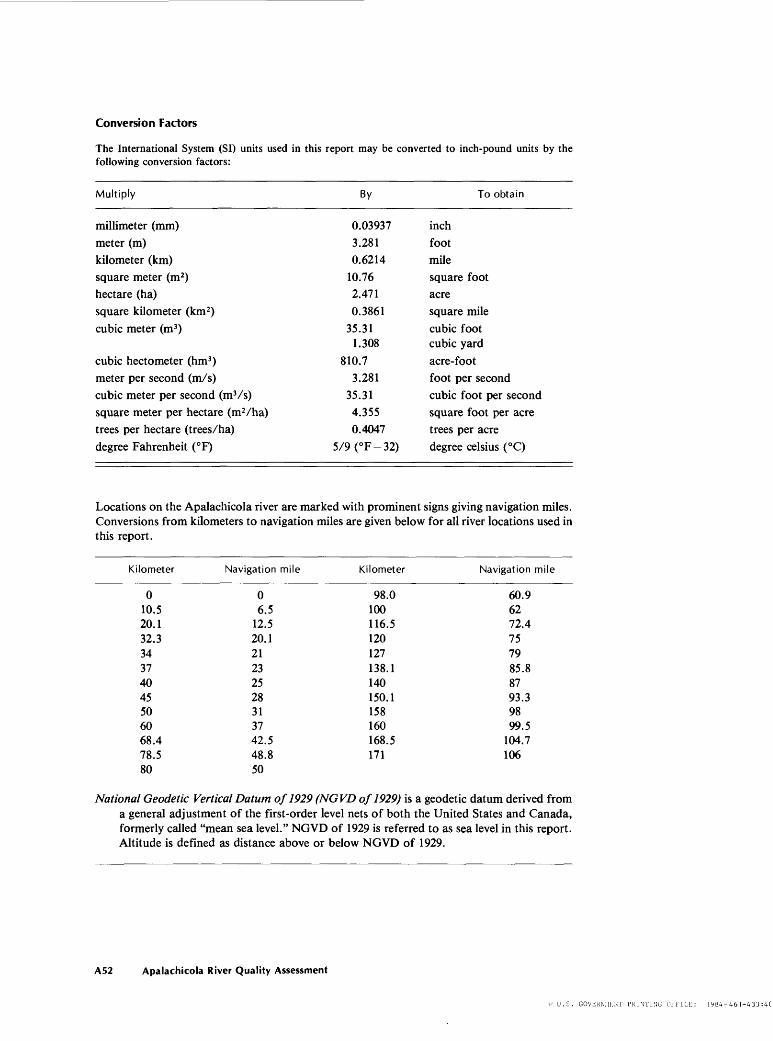
Conversion Factors

The International System (SI) units used in this report may be converted to inch-pound units by the following conversion factors:

Multiply By To obtain

millimeter (mm)meter (m)kilometer (km)square meter (m2)hectare (ha)square kilometer (km2)cubic meter (m3 )

cubic hectometer (hm3 )meter per second (m/s)cubic meter per second (mVs)square meter per hectare (mVha)trees per hectare (trees/ha)degree Fahrenheit (°F)

0.039373.2810.6214

10.762.4710.3861

35.311.308

810.73.281

35.314.3550.4047

5/9(°F-32)

inchfootmilesquare footacresquare milecubic footcubic yardacre-footfoot per secondcubic foot per secondsquare foot per acretrees per acredegree celsius (°C)

Locations on the Apalachicola river are marked with prominent signs giving navigation miles. Conversions from kilometers to navigation miles are given below for all river locations used in this report.

Kilometer

010.520.132.334374045506068.478.580

Navigation mile

06.5

12.520.121232528313742.548.850

Kilometer

98.0100116.5120127138.1140150.1158160168.5171

Navigation mile

60.96272.4757985.88793.39899.5

104.7106

National Geodetic Vertical Datum of 1929 (NG VD of 1929) is a geodetic datum derived from a general adjustment of the first-order level nets of both the United States and Canada, formerly called "mean sea level." NGVD of 1929 is referred to as sea level in this report. Altitude is defined as distance above or below NGVD of 1929.


33^1 Nonnai^isia do 3Hi QOOld 'NIVId - USGS

Documents

Transcript of 33^1 Nonnai^isia do 3Hi QOOld 'NIVId - USGS