3301 Topic 9 Hypothesis Testing
69
1 HYPOTHESIS TESTING .
-
Upload
brandon-lawrence -
Category
Documents
-
view
25 -
download
4
description
UTA IE 3301
Transcript of 3301 Topic 9 Hypothesis Testing
1
HYPOTHESIS TESTING
.
2
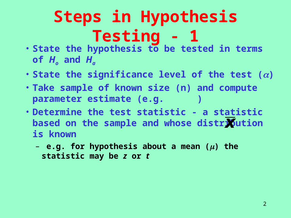
Steps in Hypothesis Testing - 1• State the hypothesis to be tested in terms of Ho and
Ha
• State the significance level of the test ()• Take sample of known size (n) and compute
parameter estimate (e.g. )• Determine the test statistic - a statistic based on
the sample and whose distribution is known– e.g. for hypothesis about a mean () the statistic may
be z or t
x
3
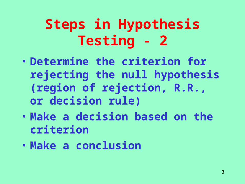
Steps in Hypothesis Testing - 2
• Determine the criterion for rejecting the null hypothesis (region of rejection, R.R., or decision rule)
• Make a decision based on the criterion
• Make a conclusion
4
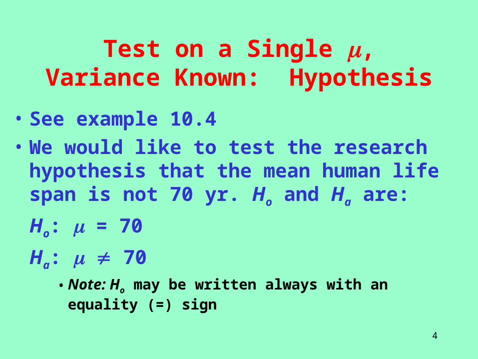
Test on a Single , Variance Known: Hypothesis
• See example 10.4
• We would like to test the research hypothesis that the mean human life span is not 70 yr. Ho and Ha are:
Ho: = 70
Ha: 70• Note: Ho may be written always with an equality (=) sign
5
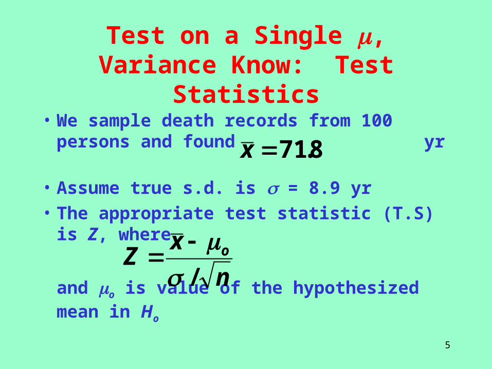
Test on a Single , Variance Know: Test Statistics
• We sample death records from 100 persons and found yr
• Assume true s.d. is = 8.9 yr
• The appropriate test statistic (T.S) is Z, where
and o is value of the hypothesized mean in Ho
8.71x
n
xZ o
/
6
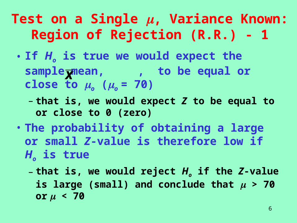
Test on a Single , Variance Known:Region of Rejection (R.R.) - 1
• If Ho is true we would expect the sample mean, , to be equal or close to o (o = 70)
– that is, we would expect Z to be equal to or close to 0 (zero)
• The probability of obtaining a large or small Z-value is therefore low if Ho is true
– that is, we would reject Ho if the Z-value is large (small) and conclude that > 70 or < 70
x
7
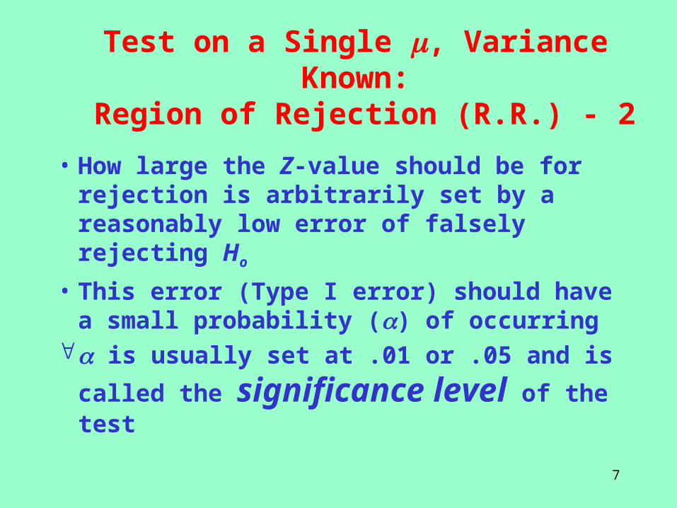
Test on a Single , Variance Known: Region of Rejection (R.R.) - 2
• How large the Z-value should be for rejection is arbitrarily set by a reasonably low error of falsely rejecting Ho
• This error (Type I error) should have a small probability () of occurring
is usually set at .01 or .05 and is called
the significance level of the test
8
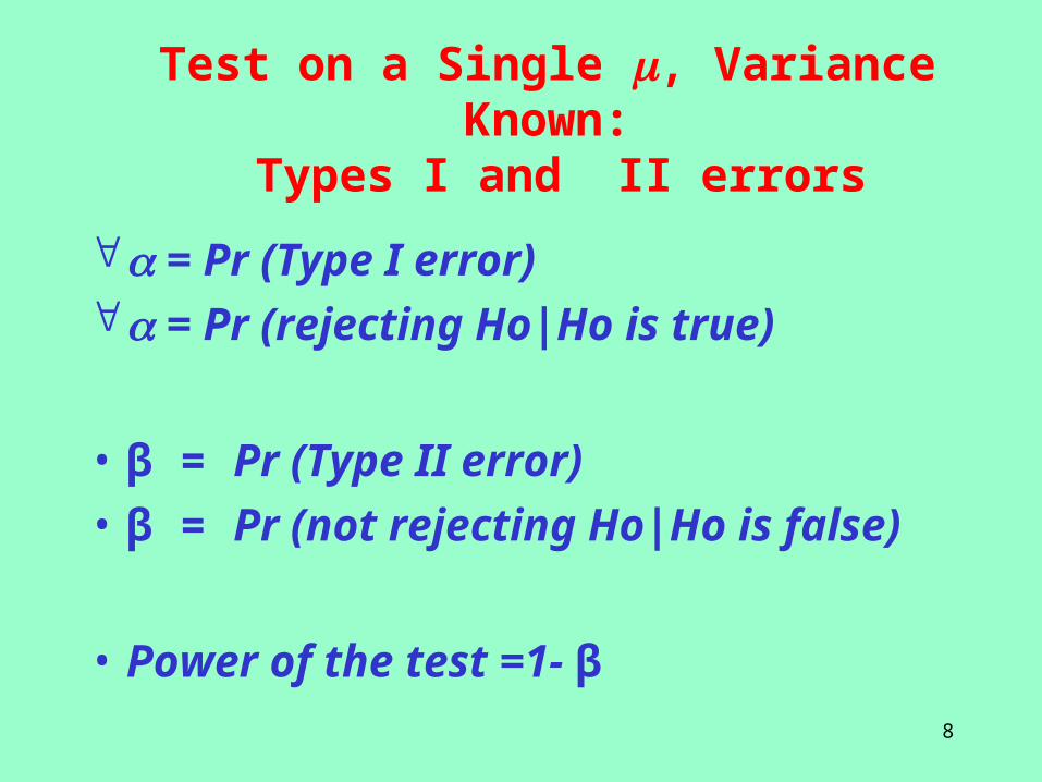
Test on a Single , Variance Known: Types I and II errors
= Pr (Type I error) = Pr (rejecting Ho|Ho is true)
• β = Pr (Type II error)
• β = Pr (not rejecting Ho|Ho is false)
• Power of the test =1- β
9
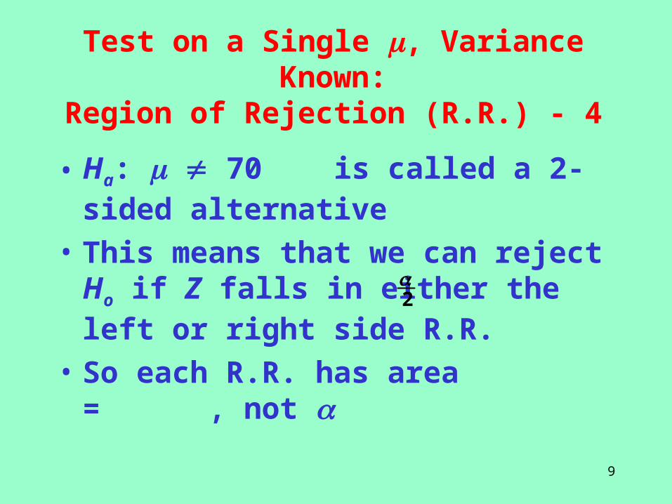
Test on a Single , Variance Known:Region of Rejection (R.R.) - 4
• Ha: 70 is called a 2-sided alternative
• This means that we can reject Ho if Z falls in either the left or right side R.R.
• So each R.R. has area = , not 2
10
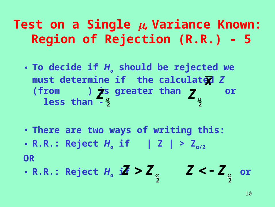
Test on a Single , Variance Known: Region of Rejection (R.R.) - 5
• To decide if Ho should be rejected we must determine if the calculated Z (from ) is greater than or less than -
• There are two ways of writing this:
• R.R.: Reject Ho if | Z | > Zα/2
OR
• R.R.: Reject Ho if or
x
2Z
2ZZ
2ZZ
2Z
11
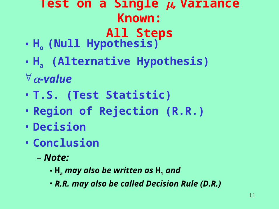
Test on a Single , Variance Known:All Steps
• Ho (Null Hypothesis)
• Ha (Alternative Hypothesis)
-value
• T.S. (Test Statistic)
• Region of Rejection (R.R.)
• Decision
• Conclusion– Note:
• Ha may also be written as H1 and
• R.R. may also be called Decision Rule (D.R.)
12
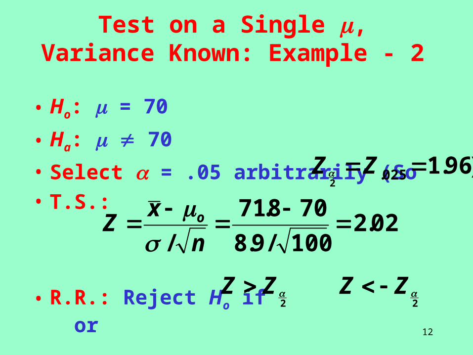
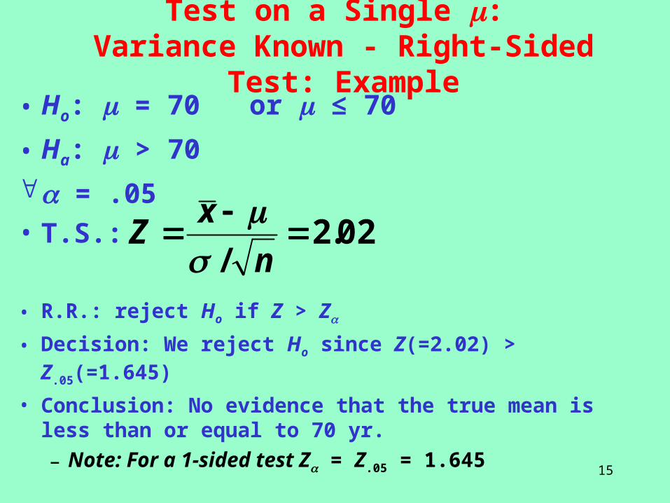
Test on a Single , Variance Known: Example - 2
• Ho: = 70
• Ha: 70
• Select = .05 arbitrarily (So
• T.S.:
• R.R.: Reject Ho if or
)96.1025.2
ZZ
02.2100/9.8
708.71
/
n
xZ o
2ZZ
2ZZ
13
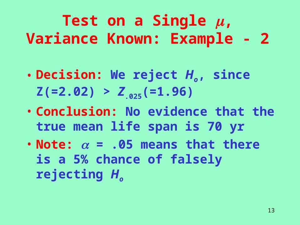
Test on a Single , Variance Known: Example - 2
• Decision: We reject Ho, since Z(=2.02) > Z.025(=1.96)
• Conclusion: No evidence that the true mean life span is 70 yr
• Note: = .05 means that there is a 5% chance of falsely rejecting Ho
14
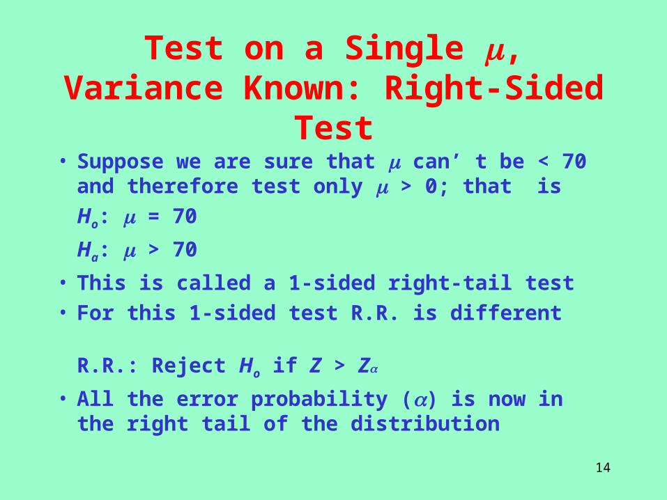
Test on a Single , Variance Known: Right-Sided Test
• Suppose we are sure that can’ t be < 70 and therefore test only > 0; that is
Ho: = 70
Ha: > 70
• This is called a 1-sided right-tail test• For this 1-sided test R.R. is different
R.R.: Reject Ho if Z > Z
• All the error probability () is now in the right tail of the distribution
15
Test on a Single : Variance Known - Right-Sided Test: Example
• Ho: = 70 or ≤ 70
• Ha: > 70
= .05
• T.S.:
• R.R.: reject Ho if Z > Z
• Decision: We reject Ho since Z(=2.02) > Z.05(=1.645)
• Conclusion: No evidence that the true mean is less than or equal to 70 yr.
– Note: For a 1-sided test Z = Z.05 = 1.645
02.2/
n
xZ
16
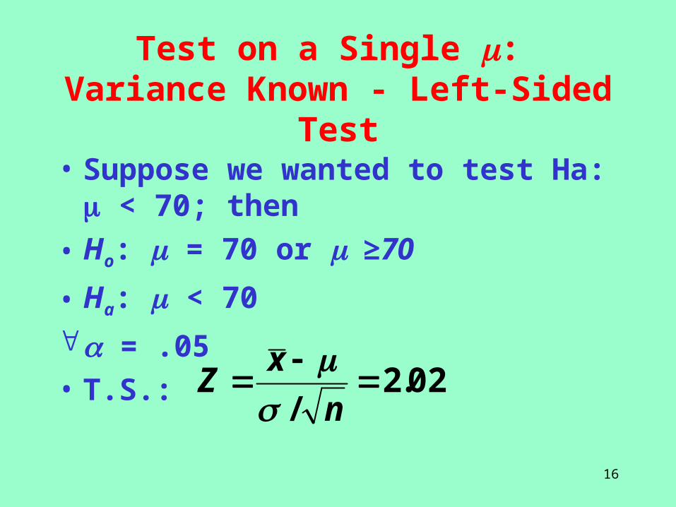
Test on a Single : Variance Known - Left-Sided Test
• Suppose we wanted to test Ha: < 70; then
• Ho: = 70 or ≥70
• Ha: < 70
= .05
• T.S.: 02.2/
n
xZ
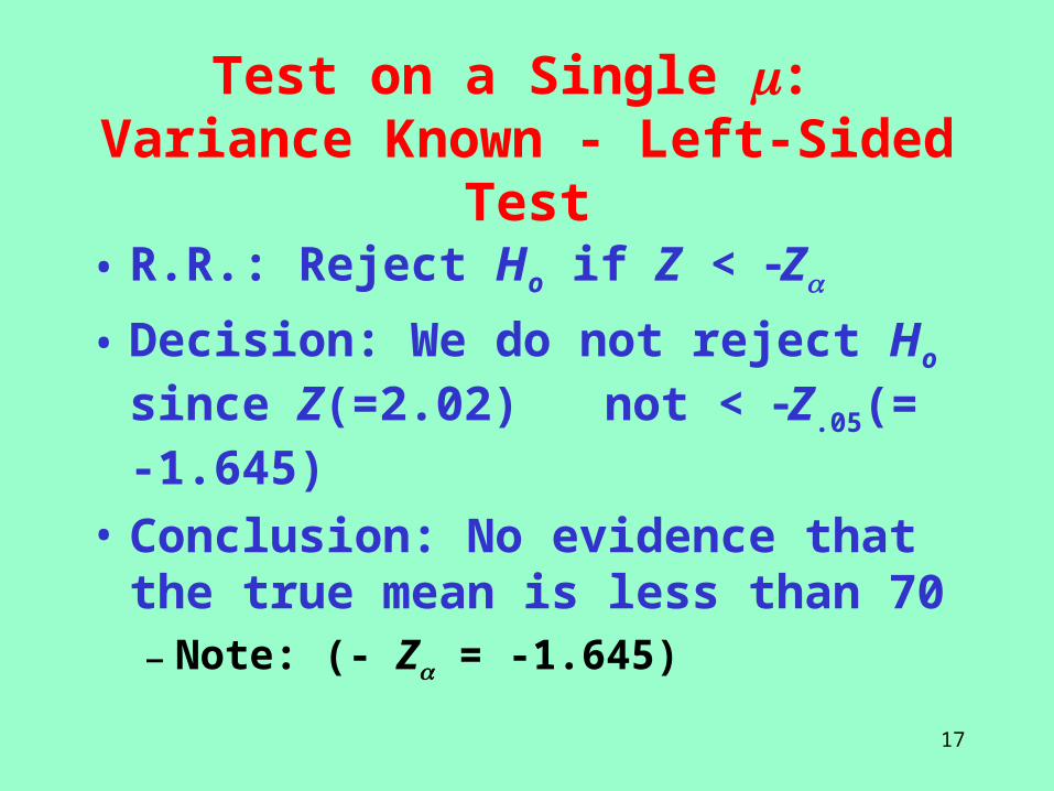
17
Test on a Single : Variance Known - Left-Sided Test
• R.R.: Reject Ho if Z < Z
• Decision: We do not reject Ho since Z(=2.02) not < Z.05(= -1.645)
• Conclusion: No evidence that the true mean is less than 70– Note: (- Z = -1.645)
18
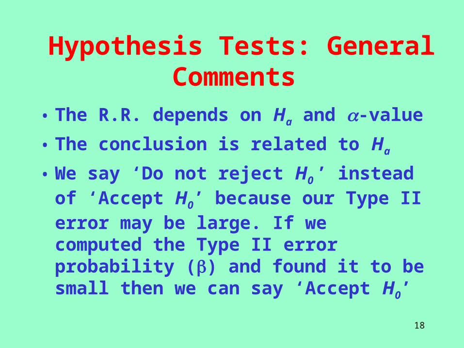
Hypothesis Tests: General Comments
• The R.R. depends on Ha and -value
• The conclusion is related to Ha
• We say ‘Do not reject H0 ’ instead of ‘Accept H0’ because our Type II error may be large. If we computed the Type II error probability () and found it to be small then we can say ‘Accept H0’

19
20
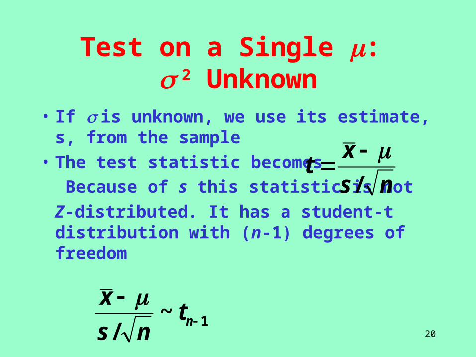
Test on a Single : 2 Unknown
• If is unknown, we use its estimate, s, from the sample
• The test statistic becomes
Because of s this statistic is not
Z-distributed. It has a student-t distribution with (n-1) degrees of freedom
ns
xt
/
1~/
ntns
x
21
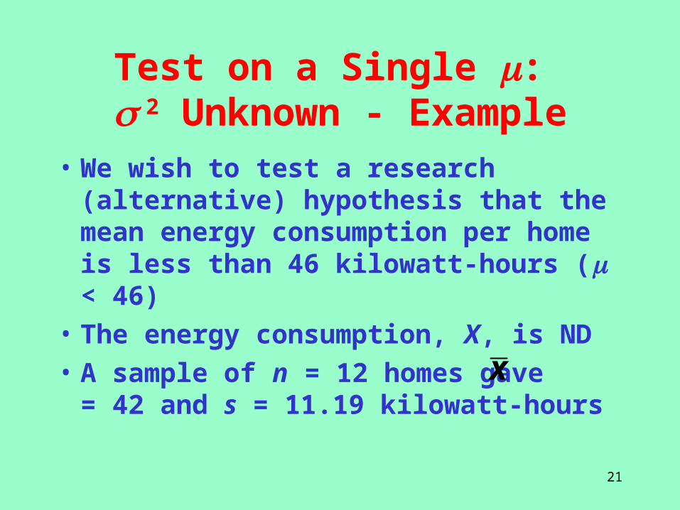
Test on a Single : 2 Unknown - Example
• We wish to test a research (alternative) hypothesis that the mean energy consumption per home is less than 46 kilowatt-hours ( < 46)
• The energy consumption, X, is ND
• A sample of n = 12 homes gave = 42 and s = 11.19 kilowatt-hours
x
22
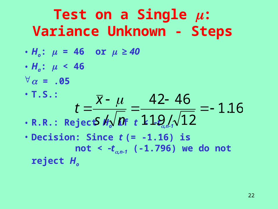
Test on a Single : Variance Unknown - Steps
• Ho: = 46 or ≥ 40
• Ha: < 46
= .05
• T.S.:
• R.R.: Reject Ho if t < t,n-1
• Decision: Since t (= -1.16) is not < t,n-1 (-1.796) we do not reject Ho
16.112/9.11
4642
/
ns
xt
23
Test on a Single : Variance Unknown - Steps
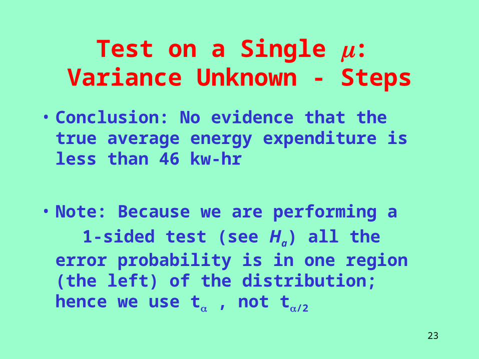
• Conclusion: No evidence that the true average energy expenditure is less than 46 kw-hr
• Note: Because we are performing a
1-sided test (see Ha) all the error probability is in one region (the left) of the distribution; hence we use t , not t/2
24
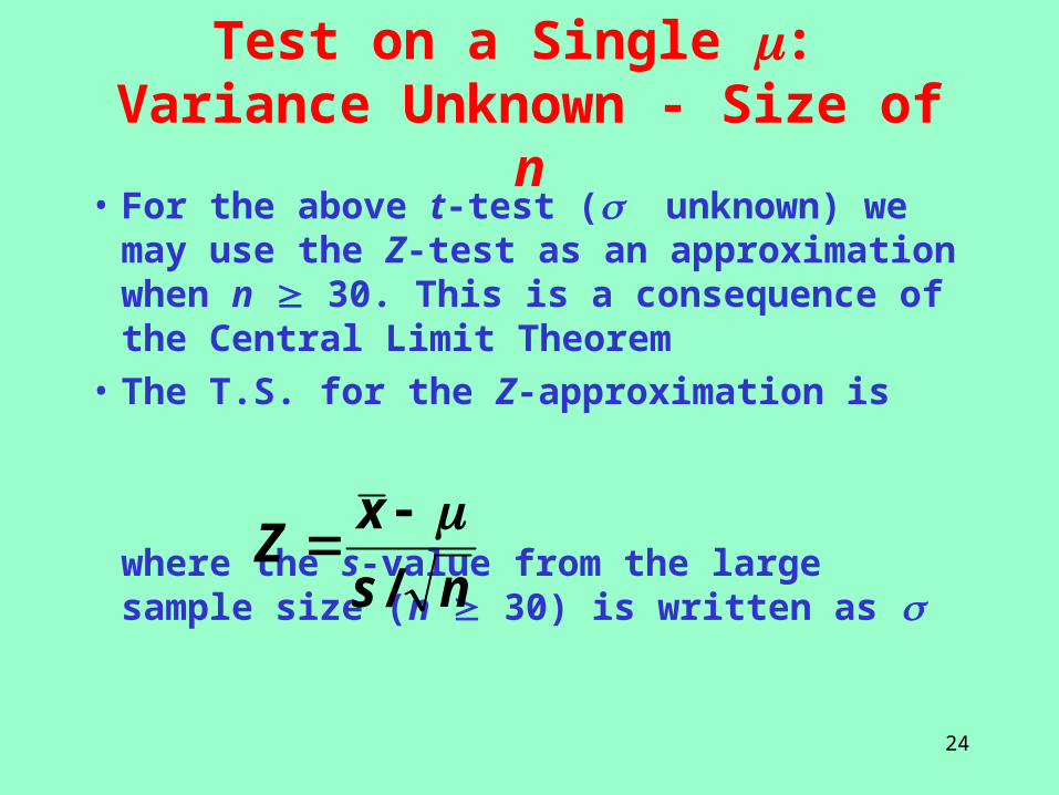
Test on a Single : Variance Unknown - Size of n
• For the above t-test ( unknown) we may use the Z-test as an approximation when n 30. This is a consequence of the Central Limit Theorem
• The T.S. for the Z-approximation is
where the s-value from the large sample size (n 30) is written as
ns
xZ
/
25
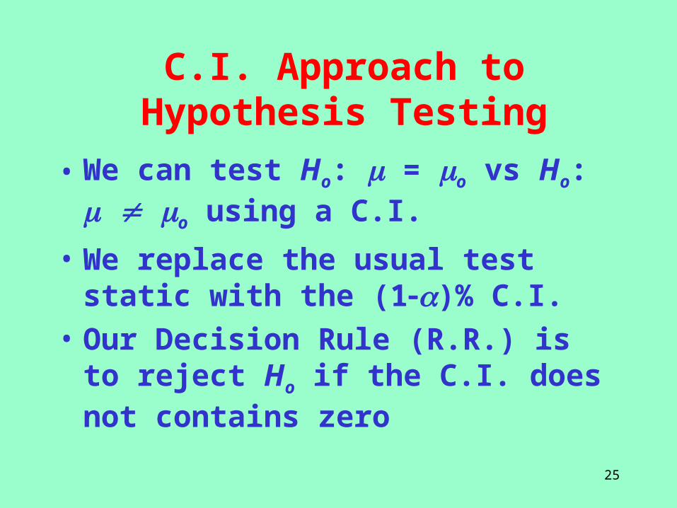
C.I. Approach to Hypothesis Testing
• We can test Ho: = o vs Ho: o using a C.I.
• We replace the usual test static with the (1)% C.I.
• Our Decision Rule (R.R.) is to reject Ho if the C.I. does not contains zero
26
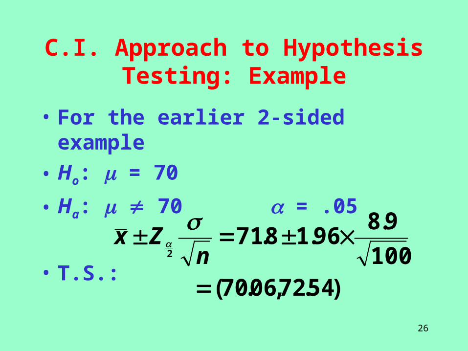
C.I. Approach to Hypothesis Testing: Example
• For the earlier 2-sided example
• Ho: = 70
• Ha: 70 = .05
• T.S.: 100
9.896.18.71
2
nZx
)54.72,06.70(
27
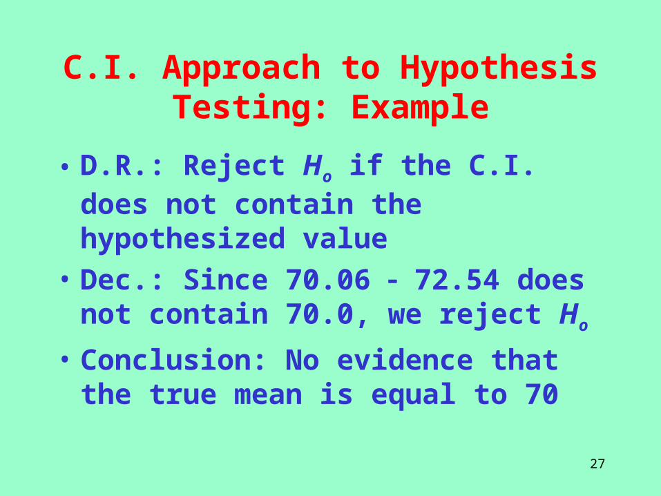
C.I. Approach to Hypothesis Testing: Example
• D.R.: Reject Ho if the C.I. does not contain the hypothesized value
• Dec.: Since 70.06 72.54 does not contain 70.0, we reject Ho
• Conclusion: No evidence that the true mean is equal to 70
28
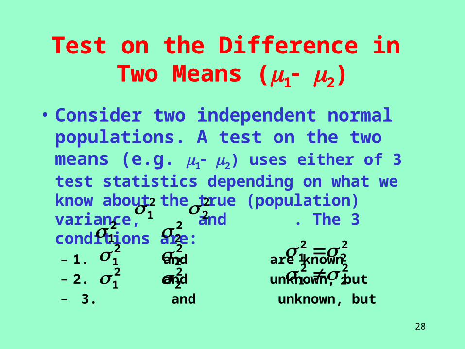
Test on the Difference in Two Means (1 2)
• Consider two independent normal populations. A test on the two means (e.g. 1 2) uses either of 3 test statistics depending on what we know about the true (population) variance, and . The 3 conditions are:– 1. and are known
– 2. and unknown, but
– 3. and unknown, but
21
2121
222222
22
21
22
21
Test on the Difference in Two Means (1 2)
21 2
2
29
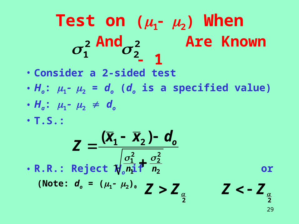
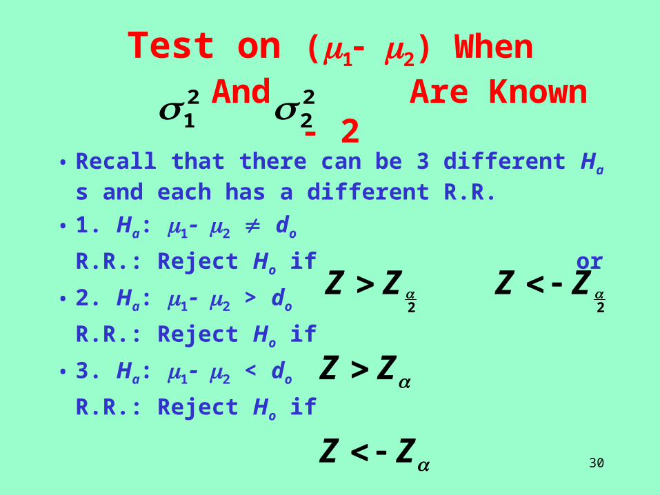
Test on (1 2) When And Are Known - 1
• Consider a 2-sided test
• Ho: 1 2 = do (do is a specified value)
• Ha: 1 2 do
• T.S.:
• R.R.: Reject Ho if or
(Note: do = (1 2)0
21 2
2
2ZZ
2ZZ
2
22
1
21
)( 21
nn
odxxZ
30
Test on (1 2) When And Are Known - 2
• Recall that there can be 3 different Ha s and each has a different R.R.
• 1. Ha: 1 2 do
R.R.: Reject Ho if or
• 2. Ha: 1 2 > do
R.R.: Reject Ho if
• 3. Ha: 1 2 < do
R.R.: Reject Ho if
2ZZ
2ZZ
ZZ
ZZ
21 2
2
31
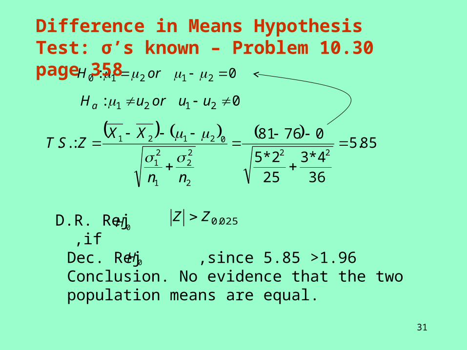
D.R. Rej ,if
0: 21210 orH
0: 2121 uuoruH a
85.5
364*3
252*5
07681:..
22
2
22
1
21
02121
nn
XXZST
0H 025.0ZZ
Dec. Rej ,since 5.85 >1.96 Conclusion. No evidence that the two population means are equal.
0H
Difference in Means Hypothesis Test: σ’s known – Problem 10.30 page 358
32
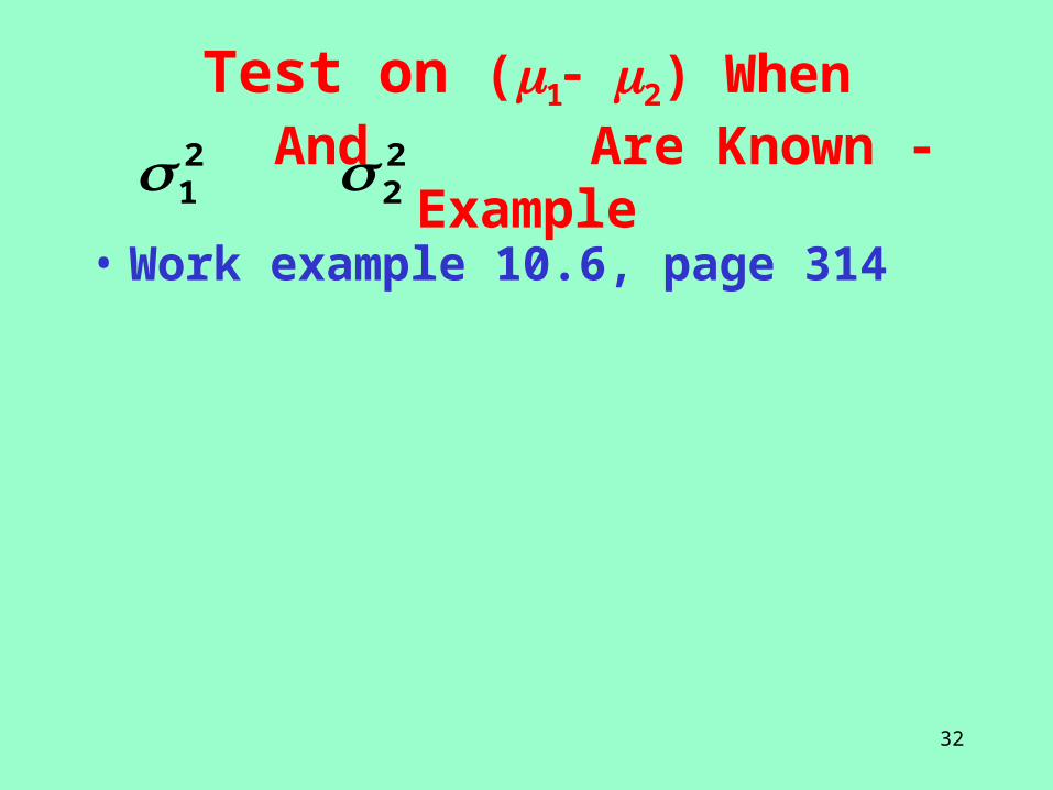
Test on (1 2) When And Are Known - Example
• Work example 10.6, page 314
21 2
2
33
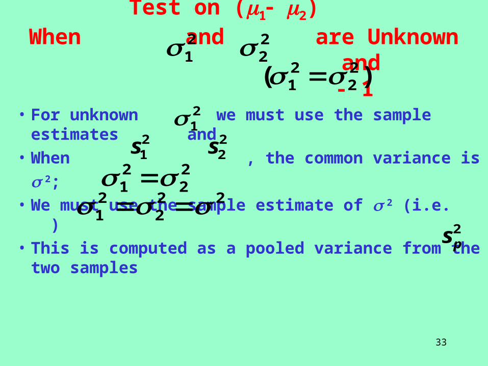
Test on (1 2) When and are Unknown
and - 1
• For unknown we must use the sample estimates and
• When , the common variance is
2;
• We must use the sample estimate of 2 (i.e. )
• This is computed as a pooled variance from the two samples
21 2
2)( 2
221
21
22s2
1s
222
21
22
21
2ps
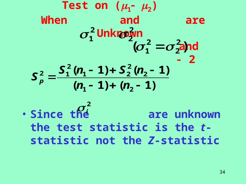
34
Test on (1 2) When and are Unknown
and - 2
• Since the are unknown the test statistic is the t-statistic not the Z-statistic
21 2
2)( 2
221
2i
)1()1(
)1()1(
21
2221
212
nn
nSnSS p
35
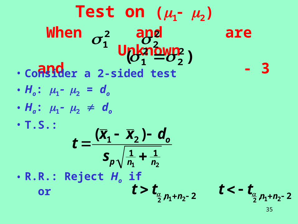
Test on (1 2) When and are Unknown
and - 3• Consider a 2-sided test
• Ho: 1 2 = do
• Ha: 1 2 do
• T.S.:
• R.R.: Reject Ho if or
21 2
2)( 2
221
21
11
21 )(
nnp
o
s
dxxt
2, 212 nntt 2, 212 nntt
36
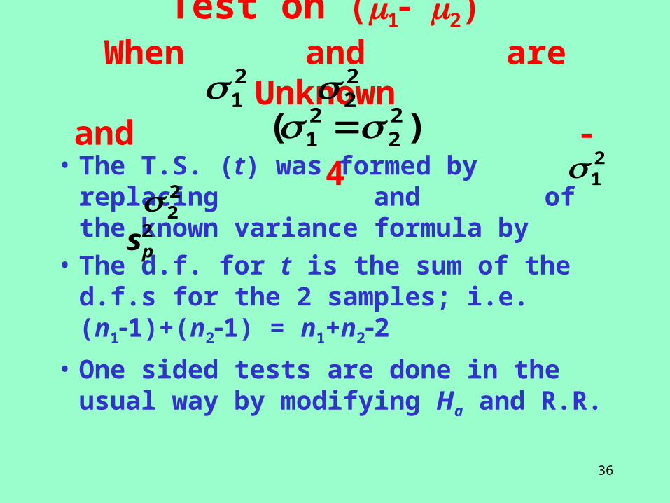
Test on (1 2) When and are Unknown
and - 4• The T.S. (t) was formed by replacing
and of the known variance formula by
• The d.f. for t is the sum of the d.f.s for the 2 samples; i.e. (n11)+(n21) = n1+n22
• One sided tests are done in the usual way by modifying Ha and R.R.
21 2
2)( 2
221
21
22
2ps
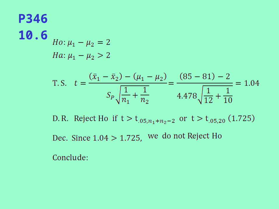
P34610.6
38
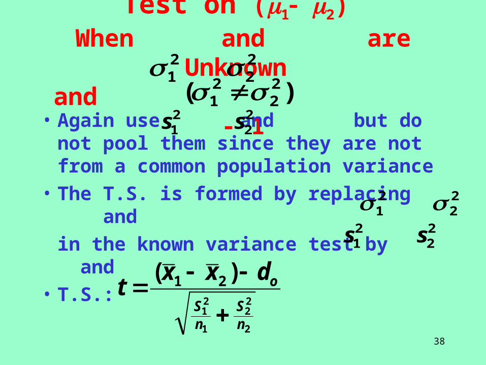
Test on (1 2) When and are Unknown
and - 1• Again use and but do not pool
them since they are not from a common population variance
• The T.S. is formed by replacing and
in the known variance test by and
• T.S.:
21 2
2)( 2
221
22s2
1s
21 2
221s 2
2s
2
22
1
21
)( 21
nS
nS
odxxt
39
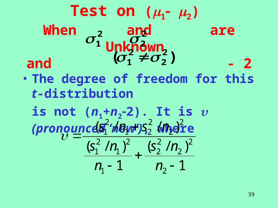
Test on (1 2) When and are Unknown
and - 2
• The degree of freedom for this t-distribution
is not (n1+n22). It is (pronounced ‘new’), where
21 2
2)( 2
221
1)/(
1)/(
)//(
2
22
22
1
21
21
22
221
21
nns
nns
nsns
40
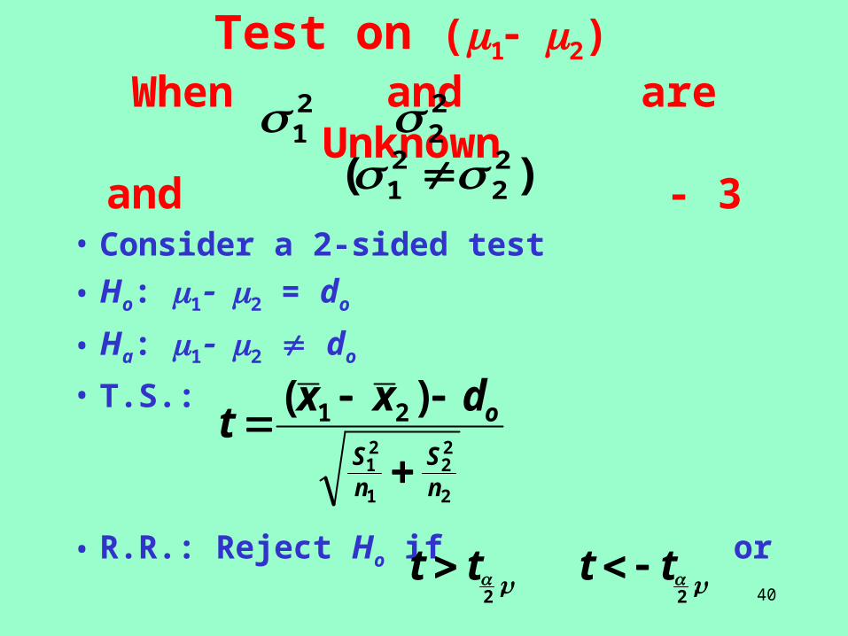
Test on (1 2) When and are Unknown
and - 3
• Consider a 2-sided test
• Ho: 1 2 = do
• Ha: 1 2 do
• T.S.:
• R.R.: Reject Ho if or
21 2
2)( 2
221
2
22
1
21
)( 21
nS
nS
odxxt
,2tt ,2
tt
41
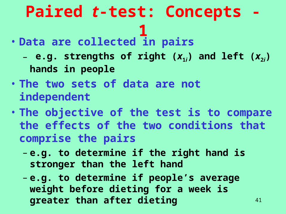
Paired t-test: Concepts - 1• Data are collected in pairs
– e.g. strengths of right (x1i) and left (x2i) hands in people
• The two sets of data are not independent
• The objective of the test is to compare the effects of the two conditions that comprise the pairs– e.g. to determine if the right hand is stronger than
the left hand– e.g. to determine if people’s average weight before
dieting for a week is greater than after dieting
42
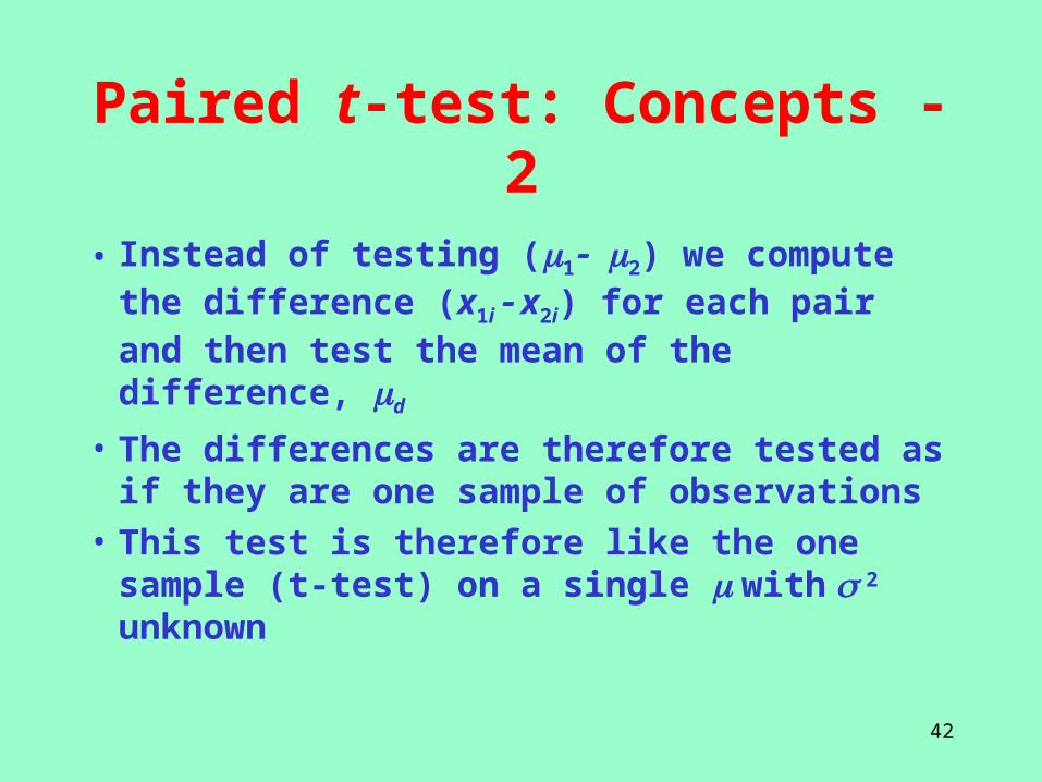
Paired t-test: Concepts - 2
• Instead of testing (1 2) we compute the difference (x1i x2i) for each pair and then test the mean of the difference, d
• The differences are therefore tested as if they are one sample of observations
• This test is therefore like the one sample (t-test) on a single with 2 unknown
43
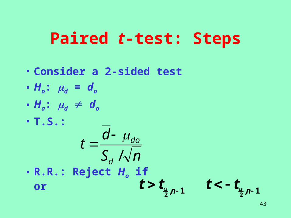
Paired t-test: Steps
• Consider a 2-sided test
• Ho: d = do
• Ha: d do
• T.S.:
• R.R.: Reject Ho if or
nS
dt
d
do
/
1,2 ntt 1,2 ntt
44
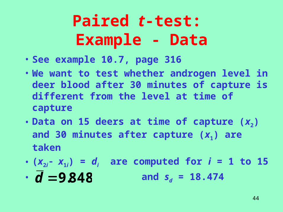
Paired t-test: Example - Data
• See example 10.7, page 316
• We want to test whether androgen level in deer blood after 30 minutes of capture is different from the level at time of capture
• Data on 15 deers at time of capture (x2) and 30 minutes after capture (x1) are taken
• (x2i x1i) = di are computed for i = 1 to 15
• and sd = 18.474848.9d
45
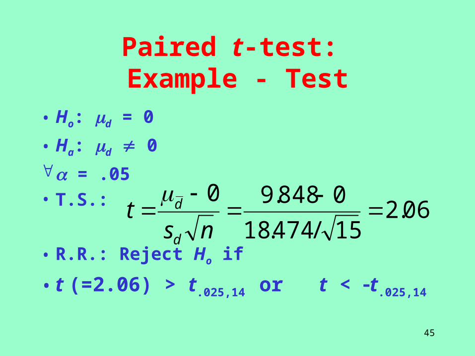
Paired t-test: Example - Test
• Ho: d = 0
• Ha: d 0
= .05• T.S.:
• R.R.: Reject Ho if
• t (=2.06) > t.025,14 or t < t.025,14
06.215/474.18
0848.90
nst
d
d
46
Paired t-test: Example- Test
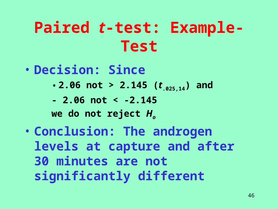
• Decision: Since • 2.06 not > 2.145 (t.025,14) and
- 2.06 not < -2.145
we do not reject Ho
• Conclusion: The androgen levels at capture and after 30 minutes are not significantly different
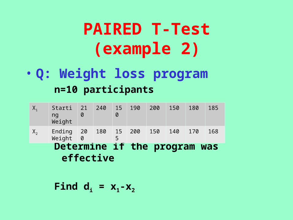
PAIRED T-Test(example 2)
• Q: Weight loss programn=10 participants
Determine if the program was effective
Find di = x1-x2
X1 Starting Weight
210 240 150 190 200 150 180 185
X2 Ending Weight
200 180 155 200 150 140 170 168
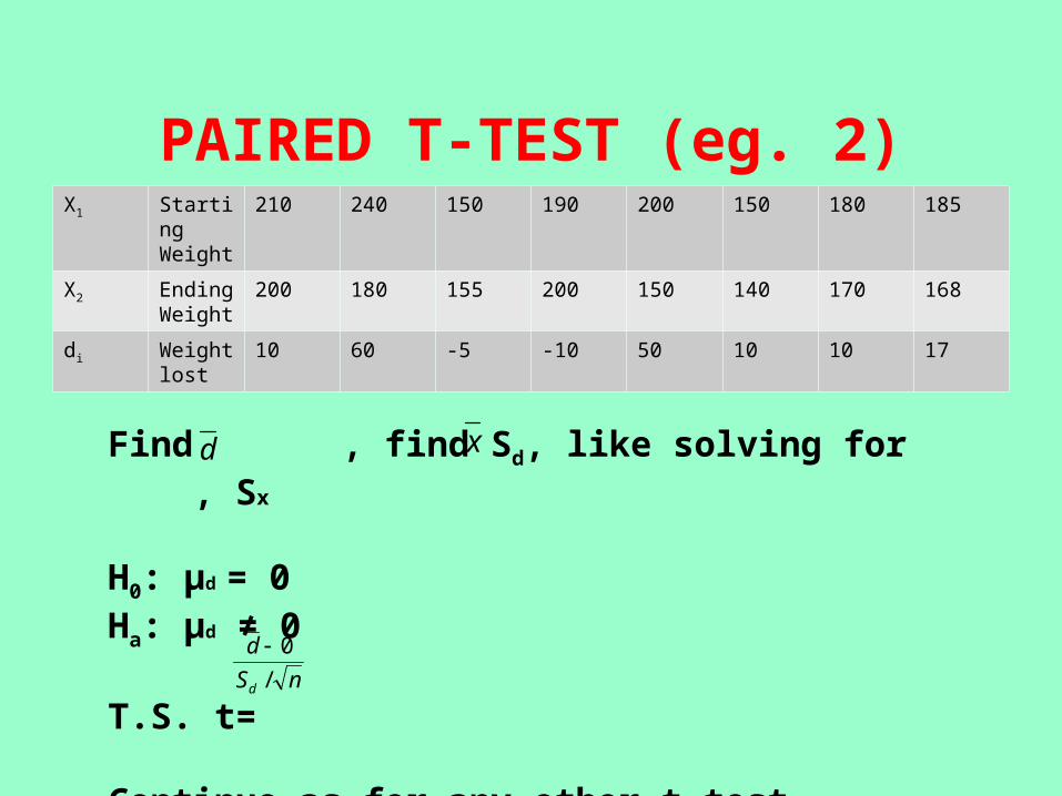
PAIRED T-TEST (eg. 2)X1 Starting
Weight210 240 150 190 200 150 180 185
X2 Ending Weight
200 180 155 200 150 140 170 168
di Weight lost
10 60 -5 -10 50 10 10 17
Find , find Sd, like solving for , Sx
H0: µd = 0Ha: µd ≠ 0
T.S. t=
Continue as for any other t-test
d x
nS
d
d /
0
49
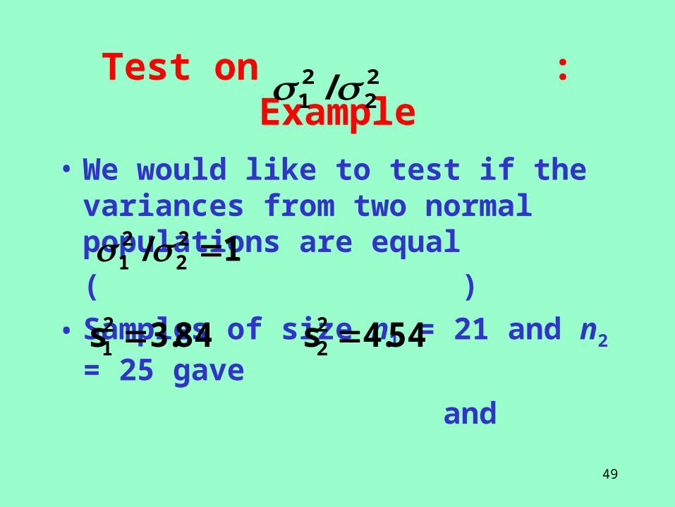
Test on : Example
• We would like to test if the variances from two normal populations are equal
( )
• Samples of size n1 = 21 and n2 = 25 gave
and
22
21 /
1/ 22
21
84.3s21 54.4s2
2
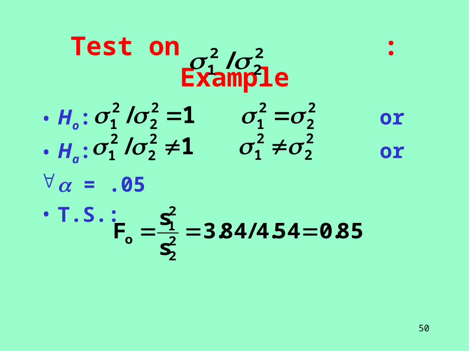
50
Test on : Example
• Ho: or
• Ha: or
= .05
• T.S.:
22
21 /
1/ 22
21
85.054.4/84.3s
sF
22
21
o
22
21
1/ 22
21 2
221
51
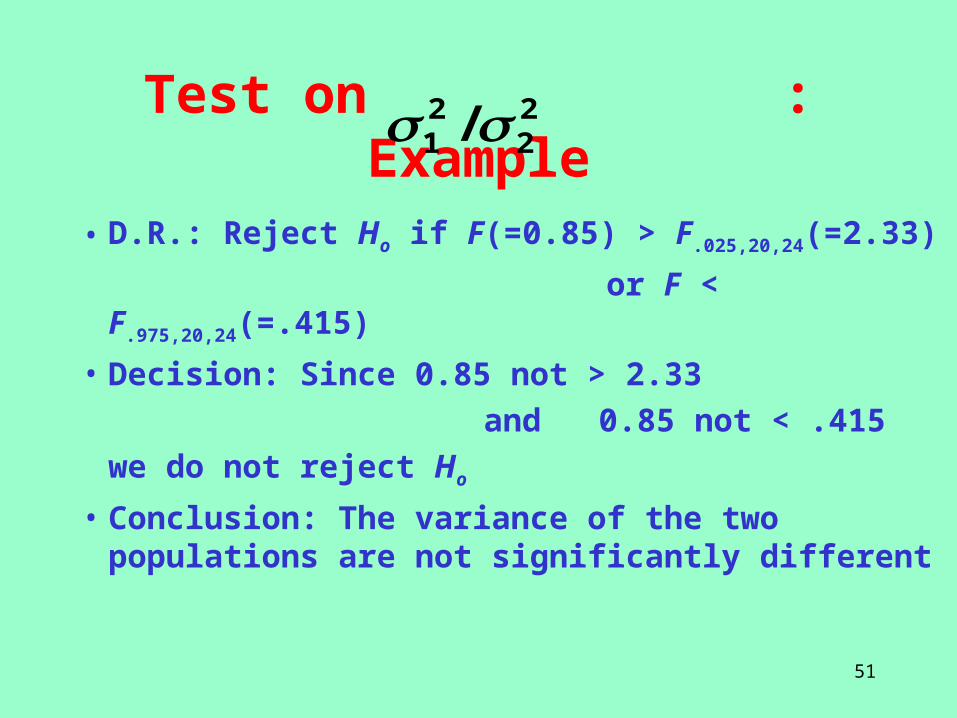
Test on : Example
• D.R.: Reject Ho if F(=0.85) > F.025,20,24(=2.33)
or F < F.975,20,24(=.415)
• Decision: Since 0.85 not > 2.33
and 0.85 not < .415
we do not reject Ho
• Conclusion: The variance of the two populations are not significantly different
22
21 /
52
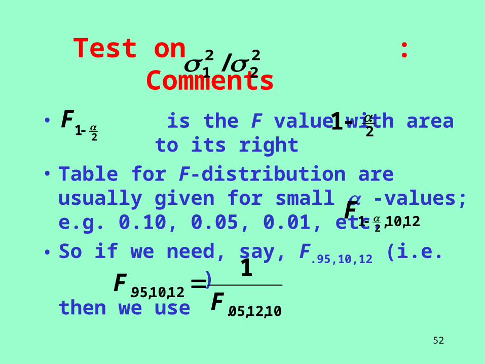
Test on : Comments
• is the F value with area to its right
• Table for F-distribution are usually given for small -values; e.g. 0.10, 0.05, 0.01, etc.
• So if we need, say, F.95,10,12 (i.e. )
then we use
22
21 /
21 F21
12,10,1 2F
10,12,05.12,10,95.
1
FF

53
.
• .
54
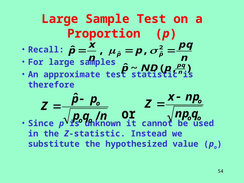
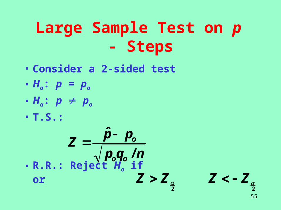
Large Sample Test on a Proportion (p)
• Recall:
• For large samples
• An approximate test statistic is therefore
• Since p is unknown it cannot be used in the Z-statistic. Instead we substitute the hypothesized value (po)
n
pqp
n
xp pp 2
ˆˆ ,,ˆ
),(~ˆnpqpNDp
nqp
ppZ
oo
o
/
ˆ
oo
o
qnp
npxZ
or
55
Large Sample Test on p - Steps
• Consider a 2-sided test
• Ho: p = po
• Ha: p po
• T.S.:
• R.R.: Reject Ho if or 2ZZ
2ZZ
nqp
ppZ
oo
o
/
ˆ
56
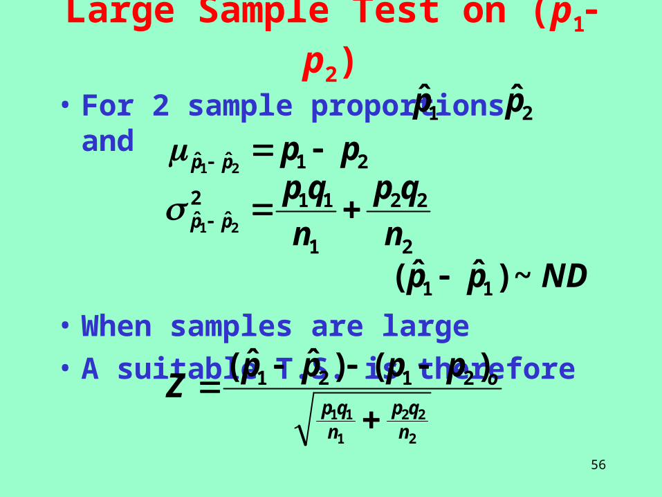
Large Sample Test on (p1 p2)
• For 2 sample proportions and
• When samples are large
• A suitable T.S. is therefore
1p̂ 2p̂
21ˆˆ 21pppp
2
22
1
112ˆˆ 21 n
qp
n
qppp
NDpp ~)ˆˆ( 11
2
22
1
11
)()ˆˆ( 2121
nqp
nqp
oppppZ
57
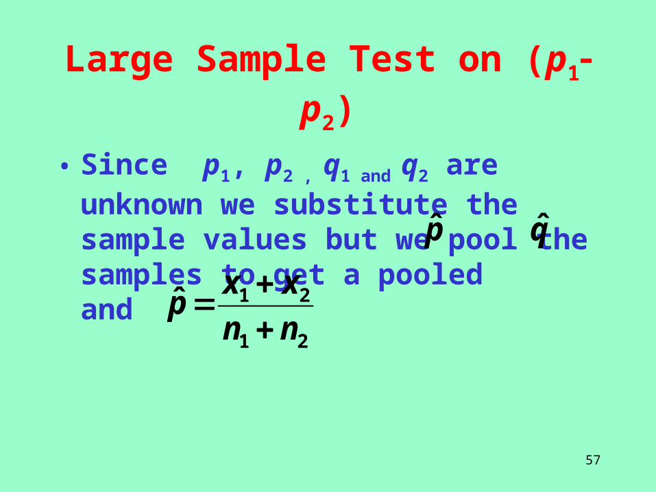
Large Sample Test on (p1 p2)
• Since p1, p2 , q1 and q2 are unknown we substitute the sample values but we pool the samples to get a pooled and p̂ q̂
21
21ˆnn
xxp
58
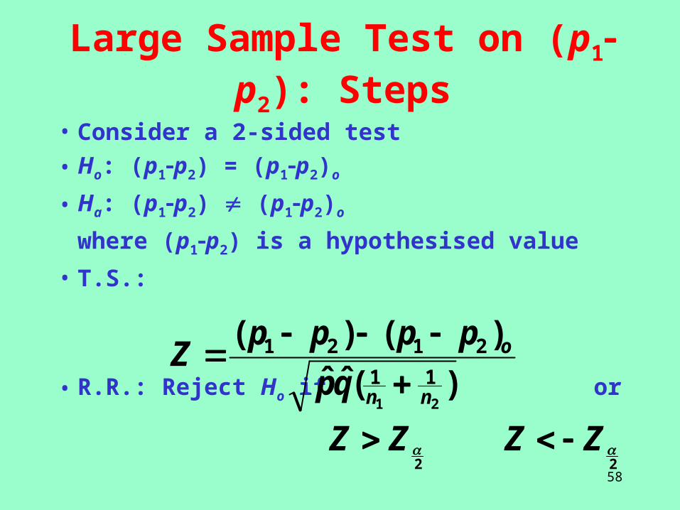
Large Sample Test on (p1 p2): Steps
• Consider a 2-sided test
• Ho: (p1p2) = (p1p2)o
• Ha: (p1p2) (p1p2)o
where (p1p2) is a hypothesised value
• T.S.:
• R.R.: Reject Ho if or )(ˆˆ
)()(
21
11
2121
nn
o
qp
ppppZ
2ZZ
2ZZ
59
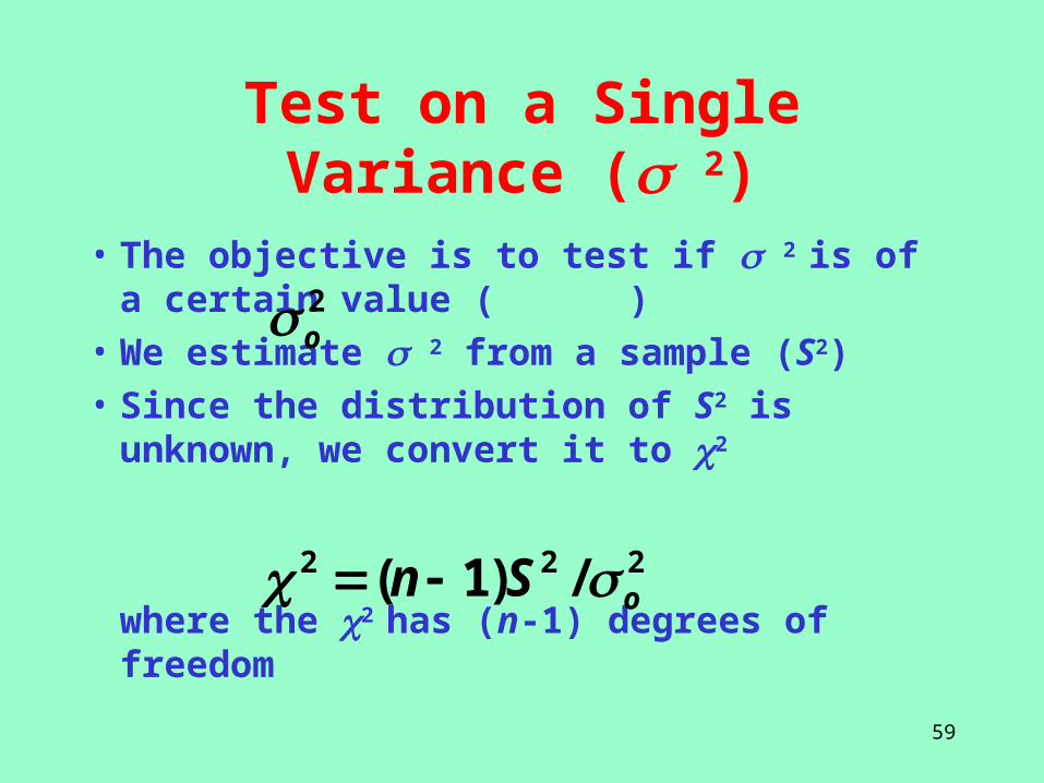
Test on a Single Variance ( 2)
• The objective is to test if 2 is of a certain value ( )
• We estimate 2 from a sample (S2)
• Since the distribution of S2 is unknown, we convert it to 2
where the 2 has (n-1) degrees of freedom
2o
222 /)1( oSn
60
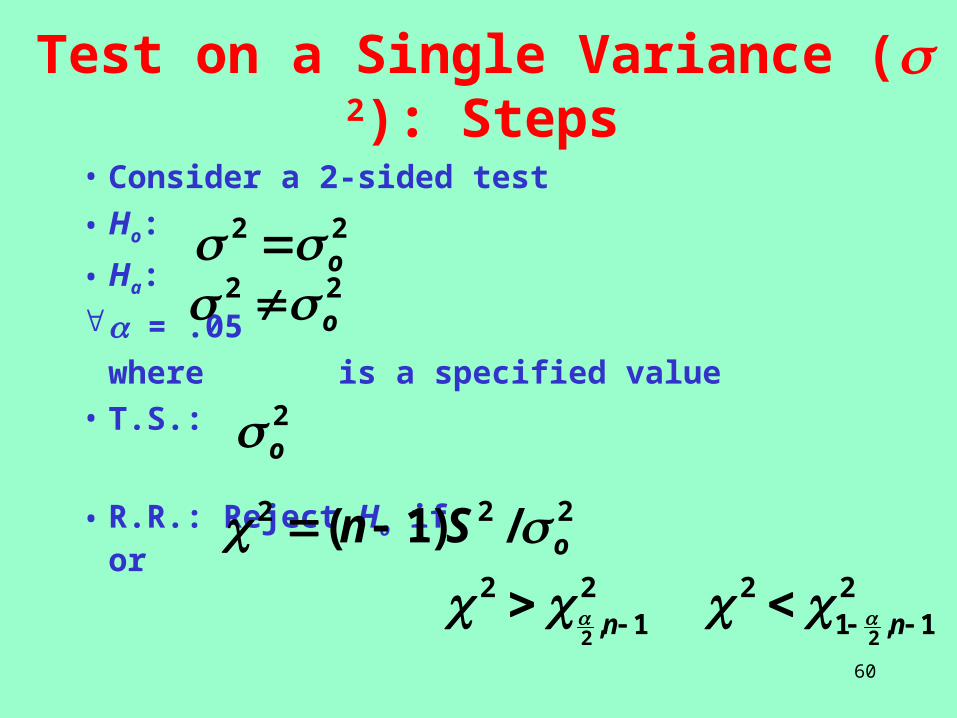
Test on a Single Variance ( 2): Steps
• Consider a 2-sided test
• Ho:
• Ha:
= .05
where is a specified value• T.S.:
• R.R.: Reject Ho if or
22o 22o
2o
222 /)1( oSn 2
1,2
2 n 21,1
2
2 n
61
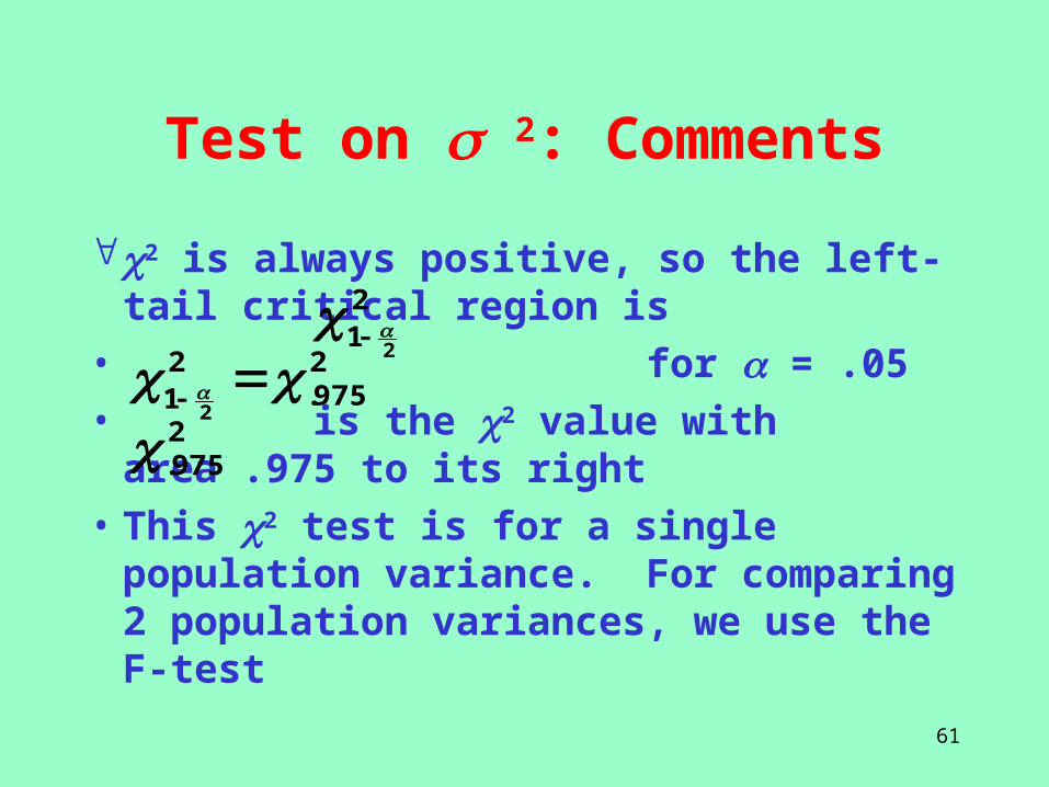
Test on 2: Comments
2 is always positive, so the left-tail critical region is
• for = .05
• is the 2 value with area .975 to its right
• This 2 test is for a single population variance. For comparing 2 population variances, we use the F-test
21 2
2975.
21 2
2975.
62
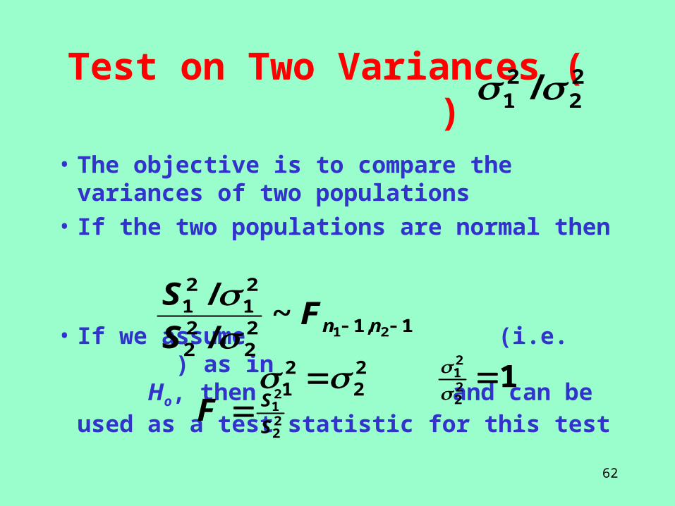
Test on Two Variances ( )
• The objective is to compare the variances of two populations
• If the two populations are normal then
• If we assume (i.e. ) as in Ho, then and can be used as a test statistic for this test
22
21 /
1,122
22
21
21
21~
/
/ nnF
S
S
22
21 12
2
21
22
21
S
SF
63
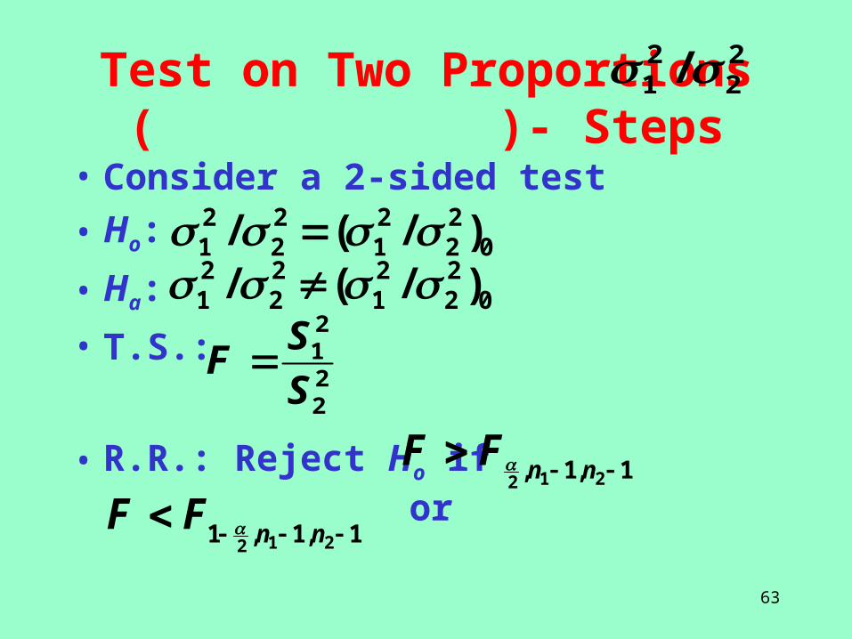
Test on Two Proportions ( )- Steps
• Consider a 2-sided test
• Ho:
• Ha:
• T.S.:
• R.R.: Reject Ho if or
22
21 /
022
21
22
21 )/(/
022
21
22
21 )/(/
22
21
S
SF
1,1, 212 nnFF
1,1,1 212 nnFF

64
.
• .
Test of Independence0 lights 1 light 2 lights 3 lights 4 lights Sums
Morning 4 6 20 65 64 159
Afternoon 8 12 20 75 72 187
Night 10 8 10 16 10 54
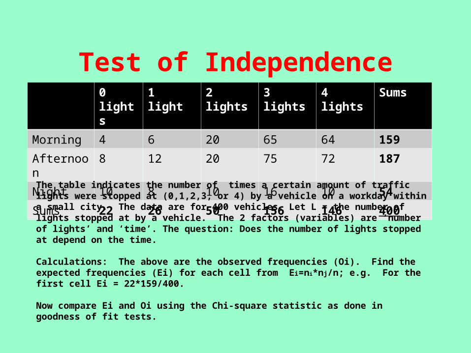
Sums 22 26 50 156 146 400The table indicates the number of times a certain amount of traffic lights were stopped at (0,1,2,3, or 4) by a vehicle on a workday within a small city. The data are for 400 vehicles. Let L = the number of lights stopped at by a vehicle. The 2 factors (variables) are ‘number of lights’ and ‘time’. The question: Does the number of lights stopped at depend on the time.
Calculations: The above are the observed frequencies (Oi). Find the expected frequencies (Ei) for each cell from Ei=ni*nj/n; e.g. For the first cell Ei = 22*159/400.
Now compare Ei and Oi using the Chi-square statistic as done in goodness of fit tests.
66
2
1
4
15
10
5
3
40
X
95.145.1 x
45.295.1 x
95.245.2 x
45.395.2 x
95.345.3 x
45.495.3 x
95.445.4 x
ii Of
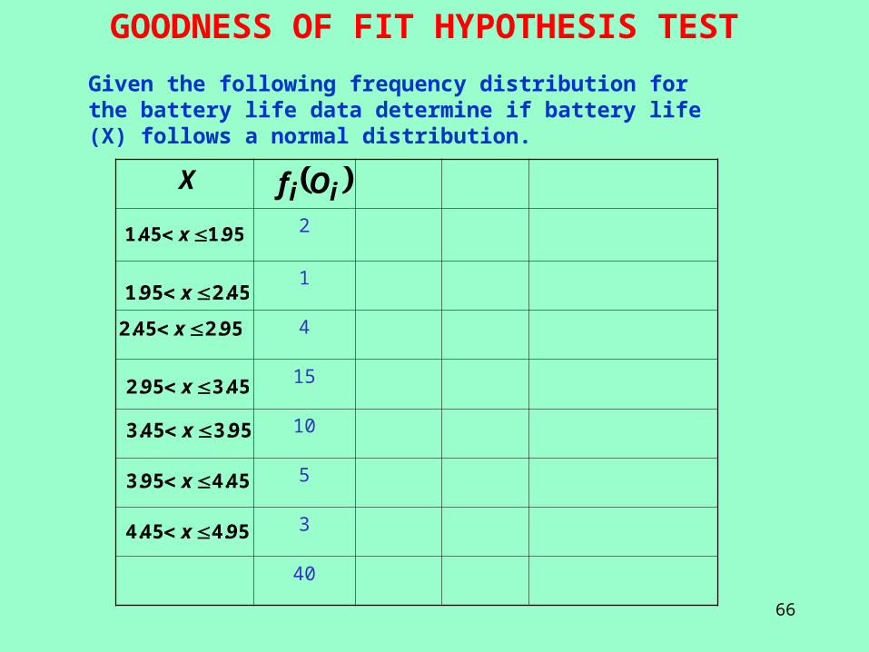
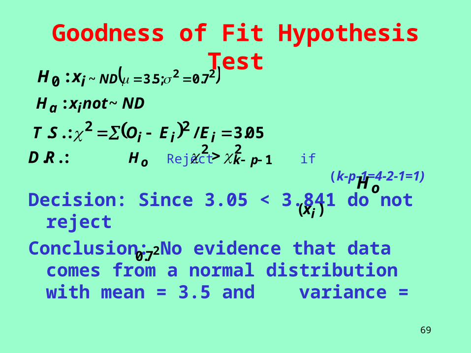
Given the following frequency distribution for the battery life data determine if battery life (X) follows a normal distribution.
GOODNESS OF FIT HYPOTHESIS TEST
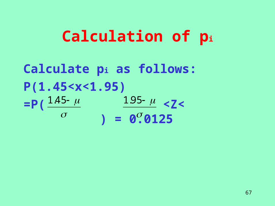
Calculation of pi
Calculate pi as follows:
P(1.45<x<1.95)
=P( <Z< ) = 0.0125
67
45.1
95.1
68
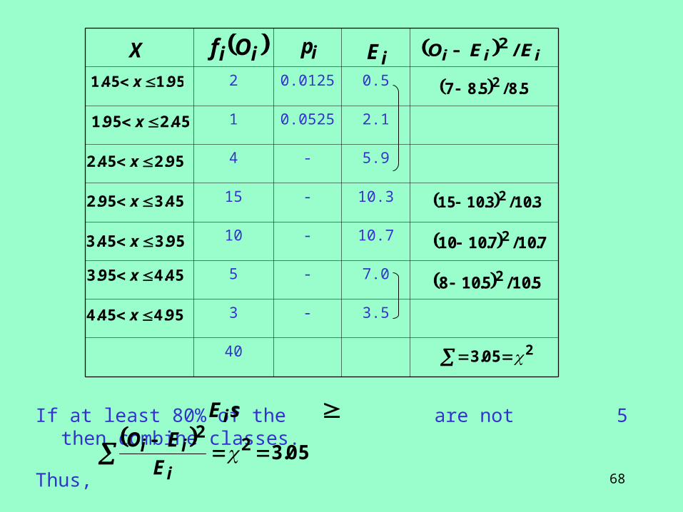
If at least 80% of the are not 5 then combine classes.
Thus,
2 0.0125 0.5
1 0.0525 2.1
4 - 5.9
15 - 10.3
10 - 10.7
5 - 7.0
3 - 3.5
40
X
95.145.1 x
45.295.1 x
95.245.2 x
45.395.2 x
95.345.3 x
45.495.3 x
95.445.4 x
ii Of ipiE iii EEO /2
5.8/5.87 2
3.10/3.1015 2
7.10/7.1010 2
5.10/5.108 2
205.3
sEi
05.322
i
iiE
EO
69
Goodness of Fit Hypothesis Test
Reject if (k-p-1=4-2-1=1)
Decision: Since 3.05 < 3.841 do not reject
Conclusion: No evidence that data comes from a normal distribution with mean = 3.5 and variance =
ixH :0 22 7.0;5.3~ ND
oH
27.0
NDnotxH ia ~:
05.3/:.. 22 iii EEOST :..RD
21
2 pkoH
)( ix