3.2: Least Squares Regressions

Section 3.2Least-Squares Regression

After this section, you should be able to…

INTERPRET a regression line

CALCULATE the equation of the least-squares regression line

CALCULATE residuals

CONSTRUCT and INTERPRET residual plots

DETERMINE how well a line fits observed data

INTERPRET computer regression output

Regression LinesA regression line summarizes the relationship between two variables, but only in settings where one of the variables helps explain or predict the other.

A regression line is a line that describes how a

response variable y changes as an explanatory variable x

changes. We often use a regression

line to predict the value of yfor a given value of x.

Regression LinesRegression lines are used to conduct analysis. • Colleges use student’s SAT and GPAs to predict

college success• Professional sports teams use player’s vital stats

(40 yard dash, height, weight) to predict success• The Federal Reserve uses economic data (GDP,

unemployment, etc.) to predict future economic trends.

• Macy’s uses shipping, sales and inventory data predict future sales.

Regression Line EquationSuppose that y is a response variable (plotted on the vertical axis) and x is an explanatory variable (plotted on the horizontal axis). A regression line relating y to x has an equation of the form:

ŷ = ax + bIn this equation,

•ŷ (read “y hat”) is the predicted value of the response variable y for a given value of the explanatory variable x.

•a is the slope, the amount by which y is predicted to change when x increases by one unit.

•b is the y intercept, the predicted value of y when x = 0.

Regression Line Equation

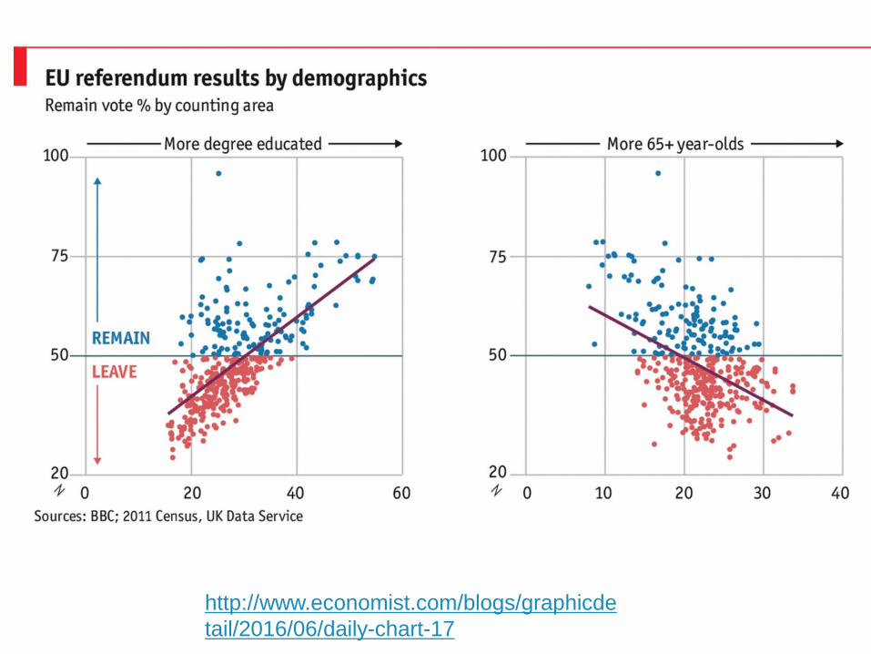
http://www.economist.com/blogs/graphicde

tail/2016/06/daily-chart-17

Format of Regression Lines

Format 1:

= 0.0908x + 16.3

= predicted back pack weight

x= student’s weight

Format 2:

Predicted back pack weight= 16.3 + 0.0908(student’s weight)

Interpreting Linear Regression• Y-intercept: A student weighing zero pounds is predicted

to have a backpack weight of 16.3 pounds (no practical interpretation).

• Slope: For each additional pound that the student weighs, it is predicted that their backpack will weigh an additional 0.0908 pounds more, on average.

Interpreting Linear Regression

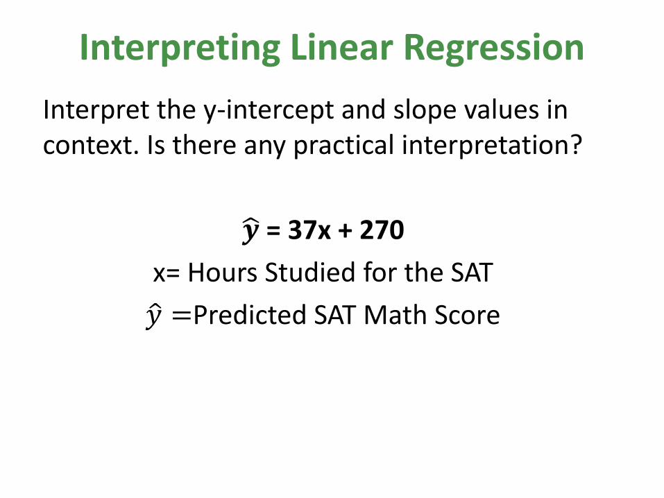
Interpret the y-intercept and slope values in context. Is there any practical interpretation?

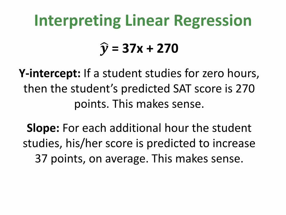
= 37x + 270

x= Hours Studied for the SAT

Predicted SAT Math Score

Interpreting Linear Regression

= 37x + 270

Y-intercept: If a student studies for zero hours, then the student’s predicted SAT score is 270

points. This makes sense.

Slope: For each additional hour the student studies, his/her score is predicted to increase

37 points, on average. This makes sense.

Predicted ValueWhat is the predicted SAT Math score for a student who studies 12 hours?

= 37x + 270

Hours Studied for the SAT (x)

Predicted SAT Math Score (y)

Predicted ValueWhat is the predicted SAT Math score for a student who studies 12 hours?

= 37x + 270

Hours Studied for the SAT (x)

Predicted SAT Math Score (y)

= 37(12) + 270

Predicted Score: 714 points

Self Check Quiz!

Self Check Quiz: Calculate the Regression Equation

A crazy professor believes that a child with IQ 100 should have a reading test score of 50, and that reading score should increase by 1 point for every additional point of IQ. What is the equation of the professor’s regression line for predicting reading score from IQ? Be sure to identify all variables used.

Self Check Quiz: Calculate the Regression Equation

A crazy professor believes that a child with IQ 100 should have a reading test score of 50, and that reading score should increase by 1 point for every additional point of IQ. What is the equation of the professor’s regression line for predicting reading score from IQ? Be sure to identify all variables used.

Answer:

= 50 + x

= predicted reading score

x = number of IQ points above 100

Self Check Quiz: Interpreting Regression Lines & Predicted Value

Data on the IQ test scores and reading test scores for a group of fifth-grade children resulted in the following regression line:

predicted reading score = −33.4 + 0.882(IQ score)

(a) What’s the slope of this line? Interpret this value in context.

(b) What’s the y-intercept? Explain why the value of the intercept is not statistically meaningful.

(c) Find the predicted reading scores for two children with IQ scores of 90 and 130, respectively.

predicted reading score = −33.4 + 0.882(IQ score)

(a) Slope = 0.882. For each 1 point increase of IQ score, the reading score is predicted to increase 0.882 points, on average.

(b) Y-intercept= -33.4. If the student has an IQ of zero, which is essential impossible (would not be able to hold a pencil to take the exam), the score would be -33.4. This has no practical interpretation.

(c) Predicted Value: 90: -33.4 + 0.882(90) = 45.98

130: -33.4 + 0.882(130) = 81.26 points.

Least-Squares Regression LineDifferent regression lines produce different residuals. The regression line we use in AP Stats is Least-Squares Regression.

The least-squares regression line of y on x is the line that makes the sum of the squared residuals as small as possible.

TI-NSpire: LSRL1. Enter x data into list 1 and y data into list 2.

2. Press MENU, 4: Statistics, 1: Stat Calculations

3. Select Option4: Linear Regression.

4. Insert either name of list or a[] for x and name of list or b[] of y. Press ENTER.

TI-NSPIRE: LSRL to View Graph

1. Enter x data into list 1 and y data into list 2. Be sure to name lists

2. Press HOME/ON, Add Data & Statistics

3. Enter variables to x and y axis.

4. Click MENU, 4: Analyze

5. Option 6: Regression

6. Option 2: Show Linear (a + bx), ENTER

ResidualsA residual is the difference between an observed value of the response variable and the value predicted by the regression line. That is,

residual = observed y – predicted y

residual = y - ŷ

residual

Positive residuals(above line)

Negative residuals(below line)

How to Calculate the Residual

1. Calculate the predicted value, by plugging in x to the LSRE.

2. Determine the observed/actual value.

3. Subtract.

Calculate the Residual1. If a student weighs 170 pounds and their backpack weighs

35 pounds, what is the value of the residual?

2. If a student weighs 105 pounds and their backpack weighs 24 pounds, what is the value of the residual?

Calculate the Residual1. If a student weighs 170 pounds and their backpack weighs 35 pounds, what is the value of the residual?

Predicted: ŷ = 16.3 + 0.0908 (170) = 31.736

Observed: 35

Residual: 35 - 31.736 = 3.264 pounds

The student’s backpack weighs 3.264 pounds more than predicted.

Calculate the Residual2. If a student weighs 105 pounds and their backpack weighs 24 pounds, what is the value of the residual?

Predicted: ŷ = 16.3 + 0.0908 (105) = 25.834

Observed: 24

Residual: 24 – 25.834= -1.834

The student’s backpack weighs 1.834 pounds less than predicted

Residual PlotsA residual plot is a scatterplot of the residuals against the explanatory variable. Residual plots help us assess how well a regression line fits the data.

TI-NSpire: Residual Plots1. Press MENU, 4: Analyze

2. Option 6: Residual, Option 2: Show Residual Plot

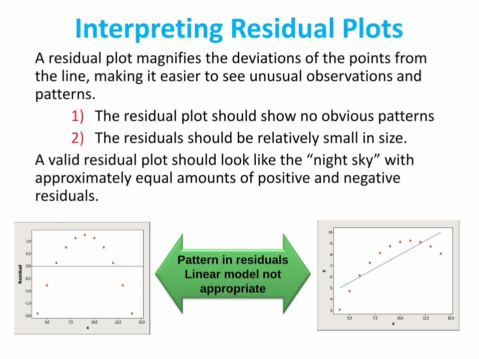
Interpreting Residual PlotsA residual plot magnifies the deviations of the points from the line, making it easier to see unusual observations and patterns.

1) The residual plot should show no obvious patterns

2) The residuals should be relatively small in size.

A valid residual plot should look like the “night sky” with approximately equal amounts of positive and negative residuals.

Pattern in residuals

Linear model not

appropriate

Should You Use LSRL?

1.

2.

Interpreting Computer Regression Output

Be sure you can locate: the slope, the y intercept and determine the equation of the LSRL.

ෝ𝒚 = -0.0034415x + 3.5051 ෝ𝒚 = predicted....x = explanatory variable

r2: Coefficient of Determinationr 2 tells us how much better the LSRL does at predicting values of ythan simply guessing the mean y for each value in the dataset.

In this example, r2 equals 60.6%.

60.6% of the variation in pack weight is explained by the linear relationship with bodyweight.

(Insert r2)% of the variation in y is explained by the linear relationship with x.

Interpret r2

Interpret in a sentence (how much variation is accounted for?)

1. r2 = 0.875, x= hours studied, y= SAT score

2. r2 = 0.523, x= hours slept, y= alertness score

Answers:

1. 87.5% of the variation in SAT score is explained by the linear relationship with the number of hours studied.

2. 52.3% of the variation in alertness score is explained by the linear relationship with the number of hours slept.

Interpret r2

S: Standard Deviation of the Residuals

1. Identify and interpret the standard deviation of the residual.

S: Standard Deviation of the Residuals

Answer:S= 0.740

Interpretation: On average, the model under predicts fat gain by 0.740 kilograms using the least-squares regression line.

S: Standard Deviation of the Residuals

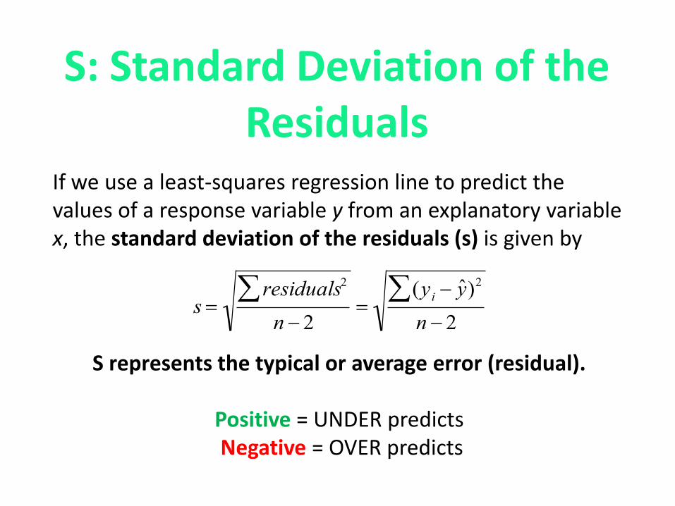
If we use a least-squares regression line to predict the values of a response variable y from an explanatory variable x, the standard deviation of the residuals (s) is given by

S represents the typical or average error (residual).

Positive = UNDER predictsNegative = OVER predicts

s residuals2

n 2

(y i ˆ y )2n 2

Self Check Quiz!The data is a random sample of 10 trains comparing number of cars on the train and fuel consumption in pounds of coal.

• What is the regression equation? Be sure to define all variables.

• What is r2 telling you?

• Define and interpret the slope in context. Does it have a practical interpretation?

• Define and interpret the y-intercept in context.

• What is s telling you?

1. ŷ = 2.1495x+ 10.667

ŷ = predicted fuel consumption in pounds of coal

x = number of rail cars

2. 96.7 % of the varation is fuel consumption is explained by the linear relationship with the number of rail cars.

3. Slope = 2.1495. With each additional car, the fuel consuption increased by 2.1495 pounds of coal, on average. This makes practical sense.

4. Y-interpect = 10.667. When there are no cars attached to the train the fuel consuption is 10.667 pounds of coal. This has no practical intrepretation beacuse there is always at least one car, the engine.

5. S= 4.361. On average, the model under predicts fuel consumption by 4.361 pounds of coal using the least-squares regression line.

ExtrapolationWe can use a regression line to predict the response ŷ for a specific value of the explanatory variable x. The accuracy of the prediction depends on how much the data scatter about the line. Exercise caution in making predictions outside the observed values of x.

Extrapolation is the use of a regression line for prediction far outside the interval of values of the explanatory

variable x used to obtain the line. Such predictions are often not accurate.

Outliers and Influential Points

• An outlier is an observation that lies outside the overall pattern of the other observations.

• An observation is influential for a statistical calculation if removing it would markedly change the result of the calculation.

• Points that are outliers in the x direction of a scatterplot are often influential for the least-squares regression line.

• Note: Not all influential points are outliers, nor are all outliers influential points.

Outliers and Influential Points

The left graph is perfectly linear. In the right graph, the last value was changed from (5, 5) to (8, 5)…clearly influential, because it changed the graph significantly. However, the residual is very small.

Correlation and Regression Limitations

The distinction between explanatory and response variables is important in regression.

Correlation and Regression Limitations

Correlation and regression lines describe only linear relationships.

NO!!!

Correlation and least-squares regression lines are not resistant.

Correlation and Regression Limitations

Correlation and Regression Wisdom

An association between an explanatory variable x and a response variable y, even if it is very strong, is not by itself good evidence that changes in x actually cause changes in y.

Association Does Not Imply Causation

A serious study once found that people with two cars live longer than people who only own one car. Owning three cars is even better, and so on. There is a substantial positive correlation between number of cars x and length of life y. Why?

Additional Calculations & Proofs

Least-Squares Regression LineWe can use technology to find the equation of the least-squares regression line. We can also write it in terms of the means and standard deviations of the two variables and their correlation.

Equation of the least-squares regression line

We have data on an explanatory variable x and a response variable y for n individuals. From the data, calculate the means and standard deviations of the two variables and their correlation. The least squares regression line is the line ŷ = a + bx with

slope and y intercept

b rsy

sx

a y bx

Calculate the Least Squares Regression Line

Some people think that the behavior of the stock market in January predicts its behavior for the rest of the year. Take the explanatory variable x to be the percent change in a stock market index in January and the response variable y to be the change in the index for the entire year. We expect a positive correlation between x and y because the change during January contributes to the full year’s change. Calculation from data for an 18-year period gives

Mean x =1.75 % Sx= 5.36% Mean y = 9.07%

Sy = 15.35% r = 0.596

Find the equation of the least-squares line for predicting full-year change from January change. Show your work.

The Role of r2 in RegressionThe standard deviation of the residuals gives us a numerical estimate of the average size of our prediction errors.

The coefficient of determination r2 is the fraction of the variation in the values of y that is accounted for by the least-squares regression line of y on x. We can calculate r2 using the following formula:

In practicality, just square the correlation r.

r2 1SSE

SST

2residualSSE 2)( yySST i

Accounted for Error

If we use the LSRL to make our predictions, the sum of the squared residuals is 30.90.SSE = 30.90

1 – SSE/SST = 1 –30.97/83.87

r2 = 0.632

63.2 % of the variation in backpack weight is accounted for by the linear model relating pack weight to body weight.

If we use the mean backpack weight as our prediction, the sum of the squared residuals is 83.87.SST = 83.87

SSE/SST = 30.97/83.87SSE/SST = 0.368

Therefore, 36.8% of the variation in pack weight is unaccounted for by the least-squares regression line.

Unaccounted for Error

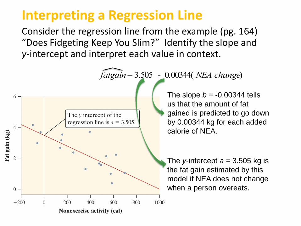
Interpreting a Regression LineConsider the regression line from the example (pg. 164) “Does Fidgeting Keep You Slim?” Identify the slope and y-intercept and interpret each value in context.

The y-intercept a = 3.505 kg is

the fat gain estimated by this

model if NEA does not change

when a person overeats.

The slope b = -0.00344 tells

us that the amount of fat

gained is predicted to go down

by 0.00344 kg for each added

calorie of NEA.

fatgain = 3.505 - 0.00344( NEA change)