3.11

Using Statistics To Make Inferences 3

Summary 

Review the normal distributionZ testZ test for the sample meant test for the sample mean

Tuesday 18 April 2023 08:41 PM

3.22

Goals To perform and interpret a Z test.To perform and interpret tests on the sample mean.To produce a confidence interval for the population mean.Know when to employ Z and when t.

 Practical  Perform a t test.

Perform a two sample t test, in preparation for next week.

3.33

Normal Distribution

0.00

0.10

0.20

0.30

0.40

0.50

0.60

0.70

0.80

-6 -4 -2 0 2 4 6

Series1

Series2

Series3

Series 1 2 3

μ 0 0 1

σ 1 ½ 1

Tables present results for the standard normal distribution (μ=0, σ=1).

3.44

Use of TablesProb(1≤z≤∞) = 68% of the observationsProb(-∞≤z≤-1) = lie within 1 standard deviation 0.16 of the mean Prob(1.96≤z≤∞) = 95% of the observations lieProb(-∞≤z≤-1.96) = within 1.96 standard

0.025 deviations of the mean

Prob(2.58≤z≤∞) = 99% of the observations lieProb(-∞≤z≤-2.58) = within 2.58 standard

0.005 deviations of the mean

3.55

Use of Tables

Z 0.00 -0.01 -0.02 -0.03 -0.04 -0.05 -0.06 -0.07 -0.08 -0.09

-1.0 0.159 0.156 0.154 0.152 0.149 0.147 0.145 0.142 0.140 0.138

-1.9 0.029 0.028 0.027 0.027 0.026 0.026 0.025 0.024 0.024 0.023

-2.5 0.006 0.006 0.006 0.006 0.006 0.005 0.005 0.005 0.005 0.005

Prob(1≤z≤∞) = Prob(-∞≤z≤-1) = 0.16

Prob(1.96≤z≤∞) = Prob(-∞≤z≤-1.96) = 0.025

Prob(2.58≤z≤∞) = Prob(-∞≤z≤-2.58) = 0.005

3.66

Testing Hypothesis

Null hypothe

sisH0

assumes that there is no real effect present

Alternate

hypothesis

H1

assumes that there is some

effect

3.77

Z Test

For a value x taken from a population with mean μ and standard deviation σ, the Z-score is

xz

3.88

The Central Limit Theorem When taking repeated samples of size n from the same population.  

3. The distribution of the sample means approximates a Normal curve.

2. The spread of the distribution of the sample means is smaller than that of the original observations.

1. The distribution of the sample means is centred around the true population mean

3.99

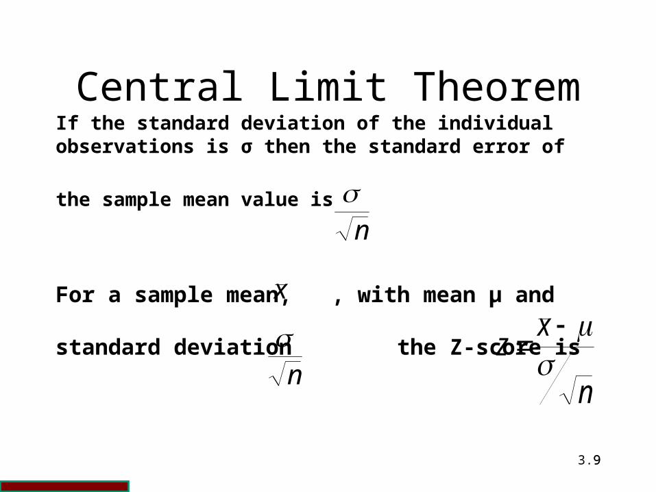
Central Limit TheoremIf the standard deviation of the individualobservations is σ then the standard error of

the sample mean value is

For a sample mean, , with mean μ and

standard deviation the Z-score is

n

x

n

n

xz

3.1010

Example 1

mean score 100 standard deviation 16What is the probability a score is higher than 108?

5.0168

16100108

x

z

Prob(x≥108) = Prob(z≥0.5) = 0.309

Z 0.00 -0.01 -0.02 -0.03 -0.04 -0.05 -0.06 -0.07 -0.08 -0.09

-0.5 0.309 0.305 0.302 0.298 0.295 0.291 0.288 0.284 0.281 0.278

3.1111

Example 2

mean score 100 standard deviation 16 The sample mean of 25 individuals is found to be 110.

The null hypothesis, no real effect present, is that μ = 100. Wish to test if the mean significantly exceeds this value.

3.1212

Solution 2125.3

2.310

2516

100110 n

xz

Prob( ≥ 100) = Prob(z≥3.125) = 0.0009, beyond our basic table

x

Z 0.00 -0.01 -0.02 -0.03 -0.04 -0.05 -0.06 -0.07 -0.08 -0.09

-3.00 .001 .001 .001 .001 .001 .001 .001 .001 .001 .001

Since the p-value is less than 0.001 the result is highly significant, the null hypothesis is rejected. The sample average is significantly higher.

3.1313

Estimating The Population Mean

Confidence interval for the population mean

 

nzx

Sample mean

n Sample size

σ Population standard deviation (known)

Tabulated value of the z-score that achieves a significance level of α in a two tail test

z

x

Don’t forget to multiply or divide before you add or subtractThis test is not available in SPSS

3.1414

Estimating The Population Mean

Confidence interval for the population mean

 

nzx

Sample mean

n Sample size

σ Population standard deviation (known)

Tabulated value of the z-score that achieves a significance level of α in a two tail test

z

x

nzx,

nzx

We can be 100(1-2α)% certain the population mean lies in the interval

3.1515

Normal Values

Conf. level

Prob. α

One Tail

Zα

90% 0.05 1.645

95% 0.025 1.960

99% 0.005 2.576Z 0.00 -0.01 -0.02 -0.03 -0.04 -0.05 -0.06 -0.07 -0.08 -0.09

-1.6 0.055 0.054 0.053 0.052 0.051 0.049 0.048 0.047 0.046 0.046

-1.9 0.029 0.028 0.027 0.027 0.026 0.026 0.025 0.024 0.024 0.023

-2.5 0.006 0.006 0.006 0.006 0.006 0.005 0.005 0.005 0.005 0.005

Notation commonly used to denote Z values for confidence interval is Zα where 100(1 - 2α) is the desired confidence level in percent.

3.1616

Example 3

standard deviation 16mean of a sample of 25 individuals is found to be 110

  Require 95% confidence interval for the population mean

110x 25n 16 96.1z

3.1717

Solution 3

110x 25n 16 96.1z

]272.116 ,728.103[25

1696.1110 n

zx

95% sure the population mean lies in the interval [103.7,116.3]

3.1818

Is there a snag?

3.1919

If The Population Standard Deviation Is Not Available?

t values

ns

tx )( with ν = n – 1 degrees of freedom(ν the Greek letter nu)

Sample mean

n Sample size

ν Degrees of freedom, n-1 in this case

s Sample standard deviation

αProportion of occasions that the true mean lies outside the range

tν Critical value of t from tables

Don’t forget to multiply or divide before you add or subtract

xNote in this module, typically, the sample variance is required. Divide by n-1

3.2020

If The Population Standard Deviation Is Not Available?

t values

Sample mean

n Sample size

ν Degrees of freedom, n-1 in this case

s Sample standard deviation

αProportion of occasions that the true mean lies outside the range

tν Critical value of t from tables

x

n

s)(tx,

n

s)(tx nn 11

3.2121

Two Tail t

To obtain confidence limits a two tail probability is employed since it refers to the proportion of values of the population mean, both above and below the sample mean.

 

3.2222

Example 4

An experiment results in the following estimates.

Obtain a 90% confidence interval for the population mean.

4.71x20n 344.7s

3.2323

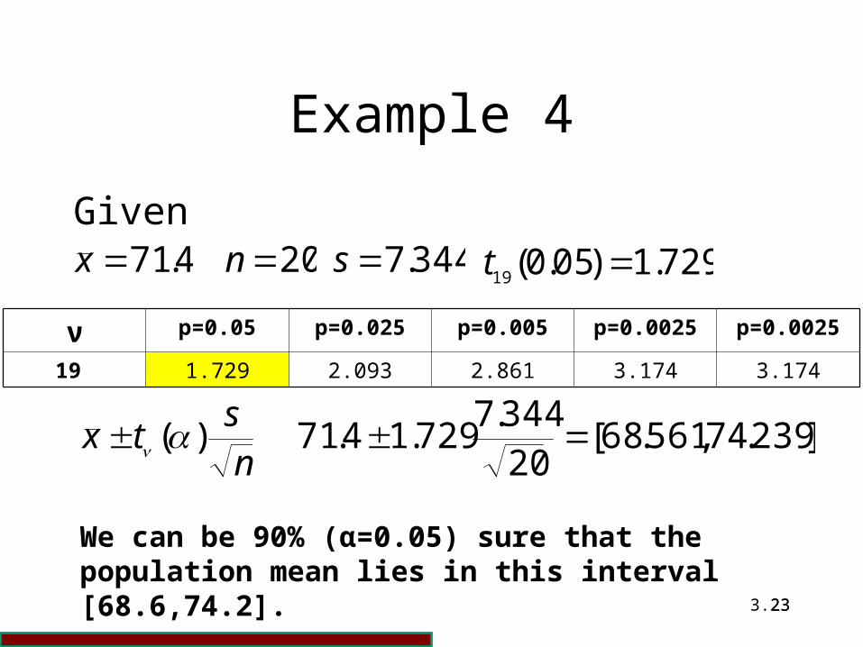
Example 4

Given4.71x 20n 344.7s 729.1)05.0(19 t

ν p=0.05 p=0.025 p=0.005 p=0.0025 p=0.0025

19 1.729 2.093 2.861 3.174 3.174

]239.74,561.68[20344.7

729.14.71 ns

tx )(

We can be 90% (α=0.05) sure that the population mean lies in this interval [68.6,74.2].

3.2424

One Sample t-Test

The basic test statistic is

nsx

t

3.2525

Interpreting t-values

If tcalc<tν(α) then we cannot reject the null hypothesis that μ=m.

 If tcalc>tν(α) the null hypothesis is rejected, the true mean μ differs significantly at the 2α level from m.

3.2626

Example 5

Claimed mean is 75 seconds, the times taken for 20 volunteers are

72 64 69 82 7670 58 64 81 7571 76 60 78 6465 73 69 84 77

H0: there is no effect so μ = 75H1: μ ≠ 75 (two tail test)

3.2727

Solution 5

n = 20 Σx = 1428 Σx2 = 102984

72 64 69 82 7670 58 64 81 7571 76 60 78 6465 73 69 84 77

n = 20 Σx = 72 + 64 + … + 84 + 77 = 1428Σx2 = 722 + 642 + … + 842 + 772 = 102984

3.2828

Solution 5

40.7120

1428... 121

n

x

n

xxxx

n

ii

n

n = 20 Σx = 1428 Σx2 = 102984

3.2929

Solution 5

40.7120

1428... 121

n

x

n

xxxx

n

ii

n

n = 20 Σx = 1428 Σx2 = 102984

s = 7.34

9368.53120

142820

1102984

1

1

var

2

2

11

2

n

xn

x

x

n

ii

n

ii

Note in this module, typically, the sample variance is required. Divide by n-1

3.3030

Solution 520n 40.71x 34.7s

193.2

2034.7

7540.71 n

sx

t

861.2)005.0(19 t 093.2)025.0(19 t

ν p=0.05 p=0.025 p=0.005 p=0.0025

p=0.0010

19 1.729 2.093 2.861 3.174 3.579

In an attempt to “estimate” p.

3.3131

Conclusion 5

Since 2.093<2.193<2.8610.01<p-value<0.05

(note 2α since two tail)

861.2)005.0(19 t 093.2)025.0(19 tt = 2.193

There is sufficient evidence to reject H0 at the 5% level. The experiment is not consistent with a mean of 75.In fact the 95% confidence interval is [68.0,74.8] which, as expected, excludes 75.

The precise p value may be found from software.

3.3232

SPSS 5Analyze > Compare Means > One Sample t Test

Note insertion of test value

3.3333

SPSS 5Basic descriptive statistics for a manual test

One-Sample Statistics

20 71.40 7.344 1.642V1N Mean Std. Deviation

Std. ErrorMean

3.3434

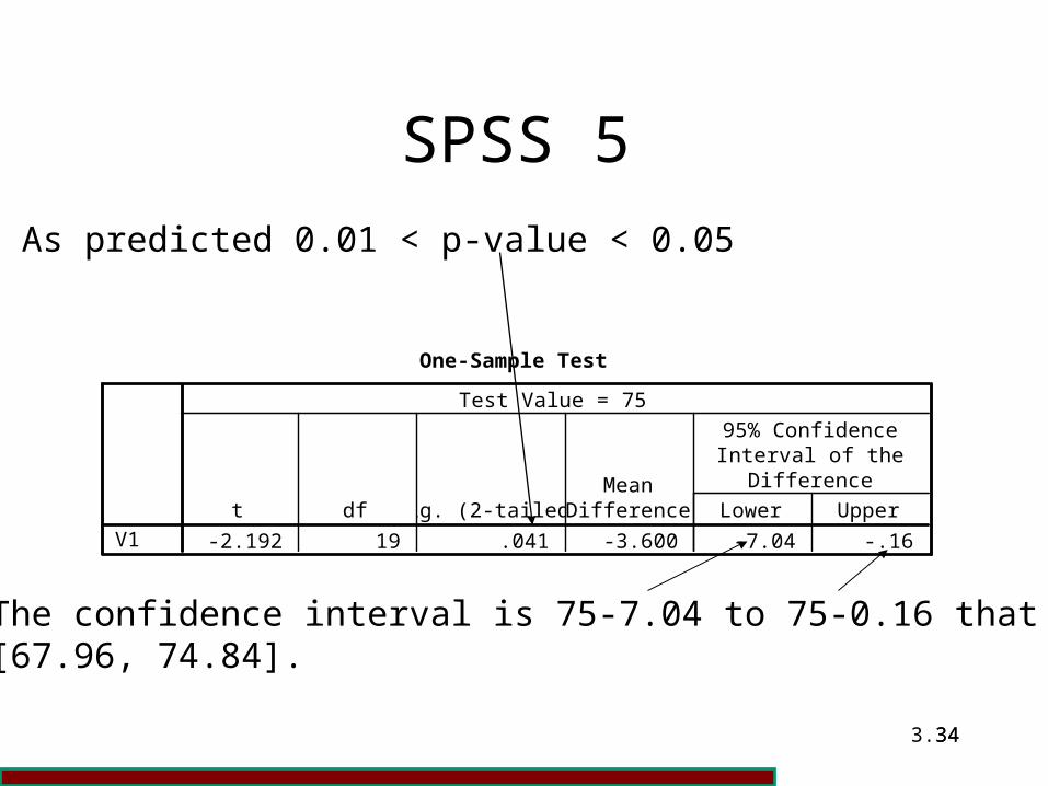
SPSS 5As predicted 0.01 < p-value < 0.05

One-Sample Test

-2.192 19 .041 -3.600 -7.04 -.16V1t df Sig. (2-tailed)

MeanDifference Lower Upper

95% ConfidenceInterval of the

Difference

Test Value = 75

The confidence interval is 75-7.04 to 75-0.16 that is [67.96, 74.84].

3.3535

Graph?Graph > Legacy Dialogs > Error Bar

3.3636

Graph? Graph > Legacy Dialogs > Error Bar

Error Bars show 95.0% Cl of Mean

68

70

72

74

V1

3.3737

Example 6

Experimental data 0.235 0.252 0.312 0.2640.323 0.241 0.284 0.3060.248 0.284 0.298 0.320

Test whether these data are consistent with a population mean of 0.250.

H0 is that μ = 0.250

3.3838

Solution 612n 2806.0x 0318.0s

333.3

120318.0

250.02806.0 n

sx

t

ν p=0.05 p=0.025 p=0.005 p=0.0025

p=0.0010

11

1.796 2.201 3.106 3.497 4.025

t11(0.005)=3.106 t11(0.0025)=3.497

In an attempt to “estimate” p.

3.3939

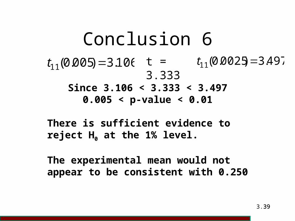
Conclusion 6106.3)005.0(11 t t = 3.333

Since 3.106 < 3.333 < 3.4970.005 < p-value < 0.01

There is sufficient evidence to reject H0 at the 1% level.

The experimental mean would not appear to be consistent with 0.250

497.3)0025.0(11 t

3.4040

SPSS 6

One-Sample Test

3.333 11 .007 .030583 .01039 .05078V1t df Sig. (2-tailed)

MeanDifference Lower Upper

95% ConfidenceInterval of the

Difference

Test Value = 0.250

As predicted p-value < 0.01

The confidence interval is 0.250+0.010 to 0.250+0.050 that is [0.26, 0.30].

3.4141

Read

Read Howitt and Cramer pages 40-50

Read Russo (e-text) pages 134-145

Read Davis and Smith pages 133-134, 139-143, 200-205, 237-264

3.4242

Practical 3

This material is available from the module web page.

http://www.staff.ncl.ac.uk/mike.cox

Module Web Page

3.4343

Practical 3

This material for the practical is available.

Instructions for the practical

Practical 3

Material for the practicalPractical 3

3.4444

Whoops!From testimony by Michael Gove, British Secretary of State for Education, before their Education Committee:

"Q98 Chair: [I]f 'good' requires pupil performance to exceed the national average, and if all schools must be good, how is this mathematically possible?

"Michael Gove: By getting better all the time.

"Q99 Chair: So it is possible, is it?

"Michael Gove: It is possible to get better all the time.

"Q100 Chair: Were you better at literacy than numeracy, Secretary of State?

"Michael Gove: I cannot remember."

Oral Evidence, British House of Commons, January 31, 2012, p. 28

3.4545

Whoops!

3.4646

Whoops!