352

Chapter Seven

Random Variables and Discrete Probability Distributions

Random Variable and Probability Distribution

• In the background, there is a random experiment. As we discussed, accompanying this experiment, we have:

• A Sample Space (all possible outcomes of the experiment)

• A probability (assigned to each outcome in the experiment)

• We now add the concept of a random variable and a probability distribution.

353

• Random Variable: A random variable is a function that assigns a number to each outcome of the experiment. 

• There are two main types of random variables: • Discrete Random Variables• Continuous Random Variables

The distinction basically depends on the range of    values that the random variable can take.

• A discrete random variable: is one that can take on  a  countable number of values. 

• A continuous random variable is one that can take on an uncountable number of values.

354

• Example: Experiment is flipping a coin 10 times, and let X=# of heads observed in the experiment. This is a discrete random variable, since X can only take on the values {0,1,2,…,10}, which is finite and therefore countable.

• Example: Suppose the experiment is measuring the time to complete a task, and let X=total time taken. This is a continuous random variable: Since time is continuous, the range of values that X can take is a continuum, and therefore uncountable. 

355

• To help understand the distinction between countable and uncountable sets, keep in mind:

a) The set of all integer numbers is countable.

b) The set of all real numbers is uncountable (a continuum).

356

Probability Distribution

• A probability distribution describes the values that a random variable can take, along with the probability associated with each value. 

• A probability distribution can be summarized by a table, a formula or a graph. 

• In Chapter 6 we focus on the probability distribution of a discrete random variable.

357

• If X is a discrete random variable, its probability distribution simply represents the probability that X can take on each one of its possible values.

• We use upper case to denote a random variable, and we use lower case to denote a particular value that this random variable can take.  

• We represent the probability that the random variable ‘X’ will equal ‘x’ as P(X=x) or, more simply, P(x). 

358

Requirements of a Discrete Probability Distribution

• As a result of the conditions required of a probability (non‐negative, they must add to 1), the probability distribution P of a discrete random variable must satisfy:

• Where the notation 

Denotes the sum of P(x) over all possible values ‘x’that the random variable X can take.

359

• Example 7.1: The Statistical Abstract of the United States is published annually. It contains a wide variety of information based on the census as well as other sources. 

• Its goal is to provide information about a variety of different aspects of the lives of the country’s residents. 

• One of the questions asks households to report the number of persons living in the household. The following table summarizes the data. 

• Develop the probability distribution of the random variable defined as the number of persons per household.

360

Number of Persons Number of Households (millions)1 31.12 38.63 18.84 16.25 7.26 2.77 or more 1.4

Total                                      116.0

361

• Probability distributions can be estimated from relative frequencies.

x P(x)       1 31.1/116.0 = .2682 38.6/116.0 = .3333 18.8/116.0 = .1624 16.2/116.0 = .1405 7.2/116.0 = .0626 2.7/116.0 = .0237 or more 1.4/116.0 = .012

Total 1.000

362

• What is the probability there are 4 or more persons in any given household?

x P(x)       1 .2682 .3333 .1624 .1405 .0626 .0237 or more .012

P(X ≥ 4) = P(4) + P(5) + P(6) + P(7 or more)= .140 + .062 + .023 + .012 = .237

363

• Example 7.2: A mutual fund salesperson has arranged to call on three people tomorrow. 

• Based on past experience the salesperson knows that there is a 20% chance of closing a sale on each call. 

• Determine the probability distribution of the number of sales the salesperson will make.

• The random variable of interest is the number of sales made. Notice that the experiment consists of calling three different clients, and that the outcomes of each call are independent of each other.

• For each call, let S denote the event “success” (i.e. closing a sale).  Past experience says that P(S)=.20. Therefore,  SC is “not closing a sale”, and P(SC)=.80

364

• We can developing the probability distribution using a Probability Tree.

P(S)=.2

P(SC)=.8P(S)=.2

P(S)=.2

P(S)=.2

P(S)=.2

P(SC)=.8

P(SC)=.8

P(SC)=.8

P(SC)=.8

S S S

S S SC

S SC S

S SC SC

SC S S

SC S SC

SC SC S

SC SC SC

P(S)=.2

P(SC)=.8

P(SC)=.8

P(S)=.2

X P(x)3 .23 = .0082 3(.032)=.0961 3(.128)=.3840 .83 = .512

(.2)(.2)(.8)= .032Sales Call 1 Sales Call 2 Sales Call 3

P(X=2) is illustrated here…365

Population/Probability Distribution…• The discrete probability distribution describes a population.

• Since we have populations, we can describe them by computing various parameters.

• Two of the population parameters we studied previously are: population mean and population variance.

366

Population Mean (Expected Value) of a Discrete Random Variable

• Our general definition of the population mean is

• If we know that the random variable X is discrete, we can re‐express µ in terms of the probability distribution of X. We have: 

• This parameter is also called the expected value of Xand is represented by E(X). 

367

Population Variance of a Discrete Random Variable• The population variance of a discrete random variable can be expressed similarly. It is the weighted average of the squared deviations from the mean:

• As before, there is a “short‐cut” formulation…

• The standard deviation is the same as before:

368

• Example 7.1 (continued): Find the mean, variance, and standard deviation for the population of X= number of persons per household. Assume that the category “7 or more” is actually 7.

• The mean E(X) is given by:

= 1(.268) + 2(.333) + 3(.162) + 4(.140) + 5(.062) + 6(.023) + 7(.012)

= 2.513

)7(7...)2(2)1(1)( PPPXE

369

• The variance of X is given by:

• The standard deviation of X is 

σ =

= (1 – 2.513)2(.268) + (2 – 2.513)2(.333)+…+(7 – 2.513)2(.012)= 1.958

399.1958.1

370

Laws of Expected Value

• There are certain properties of the Expected Value that are useful to know. Let ‘c’ be a constant. Then:

(1) E(c) = c In words: The expected value of a constant (c) is just the value of the constant.

(2) E(X + c) = E(X) + c, and (3) E(cX) = cE(X)In words:  We can “pull” a constant out of the expected value expression (either as part of a sum with a random variable X or as a coefficient of random variable X).

371

• Example 7.4: Monthly sales have a mean of $25,000 and a standard deviation of $4,000. 

• Profits are calculated by multiplying sales by 30% and subtracting fixed costs of $6,000.

Find the mean monthly profit.

1) Describe the problem statement in algebraic terms:sales have a mean of $25,000 E(Sales) = 25,000profits are calculated by…

Profit = .30(Sales) – 6,000

372

Find the mean monthly profit.

E(Profit)  =E[.30(Sales) – 6,000]=E[.30(Sales)] – 6,000 [by rule #2]=.30E(Sales) – 6,000 [by rule #3]=.30(25,000) – 6,000 = 1,500

Thus, the mean monthly profit is $1,500

373

Laws of Variance• As before, let ‘c’ be a constant. Then:

1. V(c) = 0– In words: The variance of a constant is zero (makes total sense).

2. V(X + c) = V(X)– In words:  The variance of a random variable and a constant is just the variance of the random variable (per 1 above).

3. V(cX) = c2V(X) – In words:  The variance of a random variable and a constant coefficient is the coefficient squared times the variance of the random variable.

374

Example 7.4 (continued): Monthly sales have a mean of $25,000 and a standard deviation of $4,000. Profits are calculated by multiplying sales by 30% and subtracting fixed costs of $6,000.

Find the standard deviation of monthly profits.

1) Describe the problem statement in algebraic terms:sales have a standard deviation of $4,000

V(Sales) = 4,0002 = 16,000,000(remember the relationship between standard deviation and variance                 )profits are calculated by… Profit = .30(Sales) – 6,000

375

2) The variance of profit is = V(Profit)=V[.30(Sales) – 6,000]=V[.30(Sales)] [by rule #2]=(.30)2V(Sales)  [by rule #3]=(.30)2(16,000,000) = 1,440,000

• Again, standard deviation is the square root of variance, so standard deviation of Profit = (1,440,000)1/2 = $1,200

376

• Example 7.4 (summary): Monthly sales have a mean of $25,000 and a standard deviation of $4,000. Profits are calculated by multiplying sales by 30% and subtracting fixed costs of $6,000.Find the mean and standard deviation of 

monthly profits.

• The meanmonthly profit is $1,500

• The standard deviation of monthly profit is $1,200

377

Bivariate Distributions• Up to now, we have looked at univariate distributions, that is, probability distributions in one variable.

• As you might guess, bivariate distributions are probabilities of combinations of two variables.

• Bivariate probability distributions are also called joint probability. 

• A joint probability distribution of X and Y is a table or formula that lists the joint probabilities for all pairs of values x and y, and is denoted P(x,y).

P(x,y) = P(X=x and Y=y)378

• As you might expect, the requirements for a bivariate distribution are similar to a univariate distribution, with only minor changes to the notation:

for all pairs (x,y)

379

• Example 7.5: Xavier and Yvette are real estate agents. Let X denote the number of houses that Xavier will sell in a month and let Y denote the number of houses Yvette will sell in a month. 

• An analysis of their past monthly performances has the following joint probabilities (bivariate probability distribution).

380

Marginal Probabilities• As before, we can calculate the marginal probabilities by 

summing across rows and down columns to determine the probabilities of X and Y individually:

For example: the probability that Xavier sells 1 house = P(X=1) =0.50381

Describing the Bivariate Distribution• We can describe the mean, variance, and standard deviation of each variable in a bivariate distribution by working with the marginal probabilities…

same formulae as for univariate distributions…

382

Population Covariance

• We can express the population covariance of two discrete variables in terms of their joint probability distribution as:

or alternatively using this shortcut method:

383

Coefficient of Correlation

• The (population) coefficient of correlation is calculated in the same way as described earlier…

384

• Example 7.6: Compute the covariance and the coefficient of correlation between the numbers of houses sold by Xavier and Yvette.

COV(X,Y) = (0 – .7)(0 – .5)(.12) + (1 – .7)(0 – .5)(.42) + …… + (2 – .7)(2 – .5)(.01) = –.15

= –0.15 ÷ [(.64)(.67)] = –.35

There is a weak, negative relationship between the two variables.

385

Example 7.6…

X Y Probability X - µ(x) Y - µ(y) [X - µ(x)][Y-µ(y)]0 0 0.12 -0.7 -0.5 0.0420 1 0.21 -0.7 0.5 -0.0740 2 0.07 -0.7 1.5 -0.0741 0 0.42 0.3 -0.5 -0.0631 1 0.06 0.3 0.5 0.0091 2 0.02 0.3 1.5 0.0092 0 0.06 1.3 -0.5 -0.0392 1 0.03 1.3 0.5 0.0202 2 0.01 1.3 1.5 0.020

0.7 0.5 -0.150

386

Sum of Two Variables• The bivariate distribution allows us to develop the probability distribution of any combination of the two variables. Of particular interest is the sum of two variables.

• If we consider our example of Xavier and Yvette selling houses, we can create the probability distribution of X+Y:

• From here, we can answer questions like “what is the probability that two houses are sold”?

P(X+Y=2) = P(0,2) + P(1,1) + P(2,0) = .07 + .06 + .06 = .19

387

• What is the probability that at least one house is sold between Xavier and Yvette?

• This is: Pr(X+Y ≥ 1) = P(X+Y=1)+Pr(X+Y=2)+Pr(X+Y=3)+Pr(X+Y=4)

= 0.63 + 0.19 + 0.05 + 0.01 = 0.88• What is the probability that the number of houses sold is 2 or 3?

• This is:

Pr(2 ≤ X+Y ≤ 3) = 0.19 + 0.05 = 0.24

388

Sum of Two Variables…

• Likewise, we can compute the expected value, variance, and standard deviation of X+Y in the usual way…

E(X + Y) =  0(.12) + 1(.63) + 2(.19) + 3(.05) + 4(.01) = 1.2

V(X + Y) = (0 – 1.2)2(.12) + … + (4 – 1.2)2(.01) = .56

75.56.)YX(Varyx

7.389

Laws of Expected Value and Variance for the Sum of Two Random Variables

• Previously, we stated Laws for expected values and variances involving a random variable X and a constant ‘c’. 

• We also have laws involving the sum of two random variables:

1. E(X + Y) = E(X) + E(Y)

2. V(X + Y) = V(X) + V(Y) + 2COV(X, Y)

• If X and Y are independent, COV(X, Y) = 0 and thus (2) becomes:

V(X + Y) = V(X) + V(Y)390

Example 7.5 (continued): We had already derived the marginal distributions of X and Y before. We have:

• We had obtained E(X+Y) and V(X+Y) by deriving the distribution of X+Y. But we can use the Laws of sums of random variables:

E(X + Y) = E(X) + E(Y) = .7 + .5 = 1.2V(X + Y) = V(X) + V(Y) + 2COV(X, Y)

= .41 + .45 + 2(‐.15) = .56

391

Laws of Expectation and Variance for Linear Combinations of Two Random Variables

• Let ‘c’ and ‘d’ be two constants. We can generalize the laws of expectation and variance from the sum X+Y to any linear combination

c∙X+d∙Y• We have:1. E(c∙X+d∙Y) = c∙E(X) + d∙E(Y)

2. V(c∙X+d∙Y) = c2∙ V(X) + d2∙ V(Y) + 2∙c∙d∙COV(X, Y)

• If X and Y are independent, COV(X, Y) = 0 and thus (2) becomes:

V(c∙X+d∙Y) = c2∙ V(X) + d2∙ V(Y)

392

Example: Portfolio Diversification and Asset Allocation.Consider an investor who forms a portfolio, consisting of only two stocks, by investing $4,000 in one stock and $6,000 in a second stock. Suppose that the results after 1 year are: One‐Year Results

Initial Value of Investment Rate of ReturnStock Investment After One Year on Investment1 $4,000 $5,000 R1 = .25 (25%)2 $6,000 $5,400 R2 =‐.10 (‐10%)Total $10,000 $10,400 Rp = .04 ( 4%) 

OR

Rp = w1R1 + w2R2 = (.4)(.25) + (.6)(‐.10) = .04

Percentage invested in first stock

Percentage invested in second stock

393

Mean and Variance of a Portfolio of Two Stocks• The portfolio Rp is defined as:

• Rp = w1 R1 + w2 R2• where w1 and w2 are the proportions or weights of investments 1 and 2.

• Using the laws for linear combinations of random variables, we have:E(Rp) = w1 E(R1) + w2 E(R2)V(Rp) =  w1

2 V(R1) + w22 V(R2) + 2w1w2 COV(R1, R2)

E(R1) and E(R2) are the expected values of R1 and R2, while σ1 and σ2 are their standard deviations, and ρ is the coefficient of correlation.  394

• Example 7.8: An investor has decided to form a portfolio by putting 25% of his money into McDonald’s stock and 75% into Cisco Systems stock. 

• The investor assumes that the expected returns will be 8% and 15%, respectively, and that the standard deviations will be 12% and 22%, respectively.  

a) Find the expected return on the portfolio.b) Compute the standard deviation of the returns 

on the portfolio assuming that:i. the two stocks’ returns are perfectly positively 

correlatedii. the coefficient of correlation is .5iii. the two stocks’ returns are uncorrelated

395

a) The expected values of the two stocks areE(R1) = .08 and E(R2) = .15

The weights are w1 = .25 and w2 = .75. Thus,

E(R2) = w1E(R1) + w2E(R2) = .25(.08) + .75(.15)

= .1325 

(an expected portfolio return of 13.25%)

396

The standard deviations are σ1 = .12 and σ2 = .22.  Thus,V(Rp) =  w1

2σ12 + w22σ22 + 2w1w2ρσ1σ2

= (.252)(.122) + (.752)(.222) + 2(.25)(.75)ρ (.12)(.22)= .0281 + .0099 ρ

When ρ = 1V(Rp) = .0281 + .0099(1) = .0380 

When ρ = .5V(Rp) = .0281 + .0099(.5) = .0331 

When ρ = 0V(Rp) = .0281 + .0099(0) = .0281 

397

• Next, note that the statement of the problem did not give us the covariance between R1 and R2 directly…

• However, it gave us the standard deviations of R1 and R2, and it asked us to solve the problem under three different scenarios regarding the correlation between R1 and R2.

• Recalling the formula for correlation, if we have the correlation and the standard deviations, we can recover the covariance…

398

• Recall that:

• and, therefore:

399

• Therefore, in the three correlation scenarios to be considered, we have:

(i) 1∙0.12 ∙0.22=0.0264

(ii) 0.5∙0.12 ∙0.22=0.0132

(iii) 0

400

• Recall thatV(Rp) =  w1

2 V(R1) + w22 V(R2) + 2w1w2 COV(R1, R2)

• Therefore:(i) If  = 1:V(Rp) =  0.252 0.122+ 0.752 0.222 + 2 0.25 0.75 0.0264 = 0.0380

(ii) If  = 0.5:V(Rp) =  0.252 0.122+ 0.752 0.222 + 2 0.25 0.75 0.0132 = 0.0331

(iii) If  = 0:V(Rp) =  0.252 0.122+ 0.752 0.222 + 0= 0.0281

401

Portfolio Diversification in Practice• The formulas introduced in this section require that we know the expected values, variances, and covariance (or coefficient of correlation) of the investments we’re interested in. 

• The question arises, How do we determine these parameters? The most common procedure is to estimate the parameters from historical data, using sample statistics. 

402

Portfolios with More Than Two Stocks• We can extend the formulas that describe the mean and variance of the returns of a portfolio of two stocks to a portfolio of any number of stocks.

Mean and Variance of a Portfolio of k Stocks

E(Rp ) = 

V(Rp ) =  

• Where Ri is the return of the ith stock, wi is the proportion of the portfolio invested in stock i, and k is the number of stocks in the portfolio. 

k

iii REw

1)(

k

1i

k

1ijjiji

k

1i

2i

2i )R,R(COVww2w

403

Portfolios with More Than Two Stocks• When k is greater than 2 the calculations can be tedious and time‐consuming. 

• For example, when k = 3, we need to know the values of the three weights, three expected values, three variances, and three covariances.

• When k = 4, there are four expected values, four variances and six covariances. [The number of covariances required in general is k(k‐1)/2.] 

404

Binomial Distribution• The binomial distribution is a specific example of a discrete probability distribution.

• The binomial distribution is the probability distribution that results from doing a “binomial experiment”. 

• Binomial experiments have the following properties:1) Fixed number of trials, represented as n.2) Each trial has two possible outcomes, a “success” and 

a “failure”.3) P(success)=p (and thus: P(failure)=1–p), for all trials.4) The trials are independent, which means that the 

outcome of one trial does not affect the outcomes of any other trials.

405

• “Success” and “Failure” are just labels for a binomial experiment, there is no value judgment implied.

• For example a coin flip will result in either heads or tails. If we define “heads” as success then necessarily “tails” is considered a failure.

• Other binomial experiment notions: An election candidate wins or loses An employee is male or female

406

Binomial Random VariableThe random variable of a binomial experiment is defined as the number of successes in the ‘n’ trials, and is called the binomial random variable.

• Example: flip a fair coin 10 times…

1) Fixed number of trials  n=102) Each trial has two possible outcomes  {heads (success), tails (failure)}3) P(success)= 0.50; P(failure)=1–0.50 = 0.50 4) The trials are independent  (i.e. the outcome of heads on the first flip 

will have no impact on subsequent coin flips).

• Hence flipping a coin ten times is a binomial experiment since all conditions were met.

407

Binomial Random Variable• The binomial random variable counts the number of successes in n trials of the binomial experiment. It can take on values from 0, 1, 2, …, n. Thus, its a discrete random variable.

• To calculate the probability associated with each value of X, we use combinatorics:

for x=0, 1, 2, …, n

408

• Combinatorics is a branch of mathematics which helps us “count” discrete structures  (outcomes in our case).

• n! denotes the factorial of the integer ‘n’. It is defined as:,    with  0! = 1

• Combinatoric theory tells us that the total number of different ways in which we can have ‘x’ successes in ‘n’ trials is:

• By independence of each trial, the probability of any outcome that yields ‘x’ successes in ‘n’ trials is:

409

Pr(‘x’ successes) Pr(‘n‐x’ failures)

• Thus, we have that the probability of any outcome that yields ‘x’ successes in ‘n’ trials is:         

• In addition, there are a total of  

such outcomes.

• Thus, adding up the probabilities of all such outcomes, we obtain the binomial probability formula: 

410

• Example: A quiz consists of 10 multiple‐choice questions. Each question has five possible answers, only one of which is correct. 

• Suppose a student plans to guess the answer to each question.

• What is the probability that the student gets no answers correct?

• What is the probability that the student gets two answers correct?

411

• This can be seen as a binomial experiment, where:

a) n=number of trials = 10 b) “success” of each trial is ``correctly guessing 

the answer’’.c) Each answer is independent of the others.

• Since each answer is guessed and there are five choices for each question, we have 

P(success) = 1/5 = .20

412

• Thus, we have a binomial experiment wheren=10, and P(success) = .20

• What is the probability that the student gets no answers correct? This is P(X=0):

The student has about an 11% chance of getting no answers correctusing the guessing strategy.

413

• What is the probability that the student gets two answers correct? That is, P(X=2):

Pat has about a 30% chance of getting exactly two answerscorrect using the guessing strategy.

414

Cumulative Probability• Thus far, we have been using the binomial probability distribution to find probabilities for individual values of x.

• The cumulative distribution of X at the value ‘x’ is defined as P(X ≤ x). That is, the probability that X is less than or equal to the value ‘x’.

• Suppose the quiz is failed if less than 50% of the answers are responded correctly. Find the probability that the student fails the quiz. This is Pr(X ≤ 4). This is given by:

P(X ≤ 4) = P(0) + P(1) + P(2) + P(3) + P(4)415

P(X ≤ 4) = P(0) + P(1) + P(2) + P(3) + P(4)

• We already know P(0) = .1074 and P(2) = .3020. Using the binomial formula to calculate the others:

P(1) = .2684 , P(3) = .2013, and P(4) = .0881

• We have P(X ≤ 4) = .1074 + .2684 + … + .0881 = .9672

• Thus, its about 97% probable that the student will fail the test using the luck strategy and guessing at answers…

416

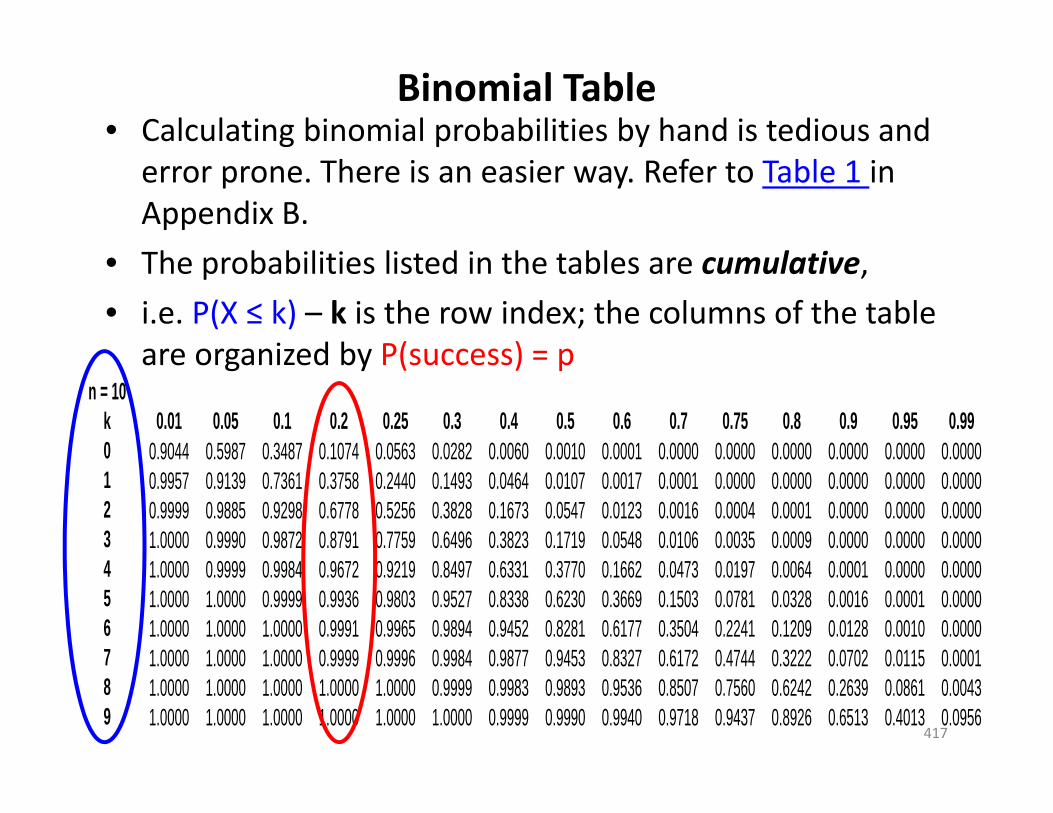
Binomial Table• Calculating binomial probabilities by hand is tedious and 

error prone. There is an easier way. Refer to Table 1 in Appendix B. 

• The probabilities listed in the tables are cumulative,• i.e. P(X ≤ k) – k is the row index; the columns of the table 

are organized by P(success) = p

417

n = 10k 0.01 0.05 0.1 0.2 0.25 0.3 0.4 0.5 0.6 0.7 0.75 0.8 0.9 0.95 0.990 0.9044 0.5987 0.3487 0.1074 0.0563 0.0282 0.0060 0.0010 0.0001 0.0000 0.0000 0.0000 0.0000 0.0000 0.00001 0.9957 0.9139 0.7361 0.3758 0.2440 0.1493 0.0464 0.0107 0.0017 0.0001 0.0000 0.0000 0.0000 0.0000 0.00002 0.9999 0.9885 0.9298 0.6778 0.5256 0.3828 0.1673 0.0547 0.0123 0.0016 0.0004 0.0001 0.0000 0.0000 0.00003 1.0000 0.9990 0.9872 0.8791 0.7759 0.6496 0.3823 0.1719 0.0548 0.0106 0.0035 0.0009 0.0000 0.0000 0.00004 1.0000 0.9999 0.9984 0.9672 0.9219 0.8497 0.6331 0.3770 0.1662 0.0473 0.0197 0.0064 0.0001 0.0000 0.00005 1.0000 1.0000 0.9999 0.9936 0.9803 0.9527 0.8338 0.6230 0.3669 0.1503 0.0781 0.0328 0.0016 0.0001 0.00006 1.0000 1.0000 1.0000 0.9991 0.9965 0.9894 0.9452 0.8281 0.6177 0.3504 0.2241 0.1209 0.0128 0.0010 0.00007 1.0000 1.0000 1.0000 0.9999 0.9996 0.9984 0.9877 0.9453 0.8327 0.6172 0.4744 0.3222 0.0702 0.0115 0.00018 1.0000 1.0000 1.0000 1.0000 1.0000 0.9999 0.9983 0.9893 0.9536 0.8507 0.7560 0.6242 0.2639 0.0861 0.00439 1.0000 1.0000 1.0000 1.0000 1.0000 1.0000 0.9999 0.9990 0.9940 0.9718 0.9437 0.8926 0.6513 0.4013 0.0956

• “What is the probability that the student gets no answers correct?” i.e. what is P(X = 0), given P(success) = .20 and n=10 ?

P(X = 0) = P(X ≤ 0) = .1074

n = 10k 0.01 0.05 0.1 0.2 0.25 0.3 0.4 0.5 0.6 0.7 0.75 0.8 0.9 0.95 0.990 0.9044 0.5987 0.3487 0.1074 0.0563 0.0282 0.0060 0.0010 0.0001 0.0000 0.0000 0.0000 0.0000 0.0000 0.00001 0.9957 0.9139 0.7361 0.3758 0.2440 0.1493 0.0464 0.0107 0.0017 0.0001 0.0000 0.0000 0.0000 0.0000 0.00002 0.9999 0.9885 0.9298 0.6778 0.5256 0.3828 0.1673 0.0547 0.0123 0.0016 0.0004 0.0001 0.0000 0.0000 0.00003 1.0000 0.9990 0.9872 0.8791 0.7759 0.6496 0.3823 0.1719 0.0548 0.0106 0.0035 0.0009 0.0000 0.0000 0.00004 1.0000 0.9999 0.9984 0.9672 0.9219 0.8497 0.6331 0.3770 0.1662 0.0473 0.0197 0.0064 0.0001 0.0000 0.00005 1.0000 1.0000 0.9999 0.9936 0.9803 0.9527 0.8338 0.6230 0.3669 0.1503 0.0781 0.0328 0.0016 0.0001 0.00006 1.0000 1.0000 1.0000 0.9991 0.9965 0.9894 0.9452 0.8281 0.6177 0.3504 0.2241 0.1209 0.0128 0.0010 0.00007 1.0000 1.0000 1.0000 0.9999 0.9996 0.9984 0.9877 0.9453 0.8327 0.6172 0.4744 0.3222 0.0702 0.0115 0.00018 1.0000 1.0000 1.0000 1.0000 1.0000 0.9999 0.9983 0.9893 0.9536 0.8507 0.7560 0.6242 0.2639 0.0861 0.00439 1.0000 1.0000 1.0000 1.0000 1.0000 1.0000 0.9999 0.9990 0.9940 0.9718 0.9437 0.8926 0.6513 0.4013 0.0956

418

• “What is the probability that the student gets two answers correct?” i.e. what is P(X = 2), given P(success) = .20 and n=10 ?

P(X = 2) = P(X≤2) – P(X≤1) = .6778 – .3758 = .3020remember, the table shows cumulative probabilities…

n = 10k 0.01 0.05 0.1 0.2 0.25 0.3 0.4 0.5 0.6 0.7 0.75 0.8 0.9 0.95 0.990 0.9044 0.5987 0.3487 0.1074 0.0563 0.0282 0.0060 0.0010 0.0001 0.0000 0.0000 0.0000 0.0000 0.0000 0.00001 0.9957 0.9139 0.7361 0.3758 0.2440 0.1493 0.0464 0.0107 0.0017 0.0001 0.0000 0.0000 0.0000 0.0000 0.00002 0.9999 0.9885 0.9298 0.6778 0.5256 0.3828 0.1673 0.0547 0.0123 0.0016 0.0004 0.0001 0.0000 0.0000 0.00003 1.0000 0.9990 0.9872 0.8791 0.7759 0.6496 0.3823 0.1719 0.0548 0.0106 0.0035 0.0009 0.0000 0.0000 0.00004 1.0000 0.9999 0.9984 0.9672 0.9219 0.8497 0.6331 0.3770 0.1662 0.0473 0.0197 0.0064 0.0001 0.0000 0.00005 1.0000 1.0000 0.9999 0.9936 0.9803 0.9527 0.8338 0.6230 0.3669 0.1503 0.0781 0.0328 0.0016 0.0001 0.00006 1.0000 1.0000 1.0000 0.9991 0.9965 0.9894 0.9452 0.8281 0.6177 0.3504 0.2241 0.1209 0.0128 0.0010 0.00007 1.0000 1.0000 1.0000 0.9999 0.9996 0.9984 0.9877 0.9453 0.8327 0.6172 0.4744 0.3222 0.0702 0.0115 0.00018 1.0000 1.0000 1.0000 1.0000 1.0000 0.9999 0.9983 0.9893 0.9536 0.8507 0.7560 0.6242 0.2639 0.0861 0.00439 1.0000 1.0000 1.0000 1.0000 1.0000 1.0000 0.9999 0.9990 0.9940 0.9718 0.9437 0.8926 0.6513 0.4013 0.0956

419

• What is the probability that the student fails the quiz”? i.e. what is P(X ≤ 4), given P(success) = .20 and n=10 ?

P(X ≤ 4) = .9672 

n = 10k 0.01 0.05 0.1 0.2 0.25 0.3 0.4 0.5 0.6 0.7 0.75 0.8 0.9 0.95 0.990 0.9044 0.5987 0.3487 0.1074 0.0563 0.0282 0.0060 0.0010 0.0001 0.0000 0.0000 0.0000 0.0000 0.0000 0.00001 0.9957 0.9139 0.7361 0.3758 0.2440 0.1493 0.0464 0.0107 0.0017 0.0001 0.0000 0.0000 0.0000 0.0000 0.00002 0.9999 0.9885 0.9298 0.6778 0.5256 0.3828 0.1673 0.0547 0.0123 0.0016 0.0004 0.0001 0.0000 0.0000 0.00003 1.0000 0.9990 0.9872 0.8791 0.7759 0.6496 0.3823 0.1719 0.0548 0.0106 0.0035 0.0009 0.0000 0.0000 0.00004 1.0000 0.9999 0.9984 0.9672 0.9219 0.8497 0.6331 0.3770 0.1662 0.0473 0.0197 0.0064 0.0001 0.0000 0.00005 1.0000 1.0000 0.9999 0.9936 0.9803 0.9527 0.8338 0.6230 0.3669 0.1503 0.0781 0.0328 0.0016 0.0001 0.00006 1.0000 1.0000 1.0000 0.9991 0.9965 0.9894 0.9452 0.8281 0.6177 0.3504 0.2241 0.1209 0.0128 0.0010 0.00007 1.0000 1.0000 1.0000 0.9999 0.9996 0.9984 0.9877 0.9453 0.8327 0.6172 0.4744 0.3222 0.0702 0.0115 0.00018 1.0000 1.0000 1.0000 1.0000 1.0000 0.9999 0.9983 0.9893 0.9536 0.8507 0.7560 0.6242 0.2639 0.0861 0.00439 1.0000 1.0000 1.0000 1.0000 1.0000 1.0000 0.9999 0.9990 0.9940 0.9718 0.9437 0.8926 0.6513 0.4013 0.0956

420

Using the Binomial Probability Table• The binomial table gives cumulative probabilities for P(X ≤ k). 

• However, we may be interested in probabilities of the type:

a) Pr(X = k)b) Pr(X ≥ k)c) Pr(k1 ≤ X ≤ k2) (with k1 < k2) 

• We can compute these probabilities from cumulative probabilities, we explain how next…

421

• If X is discrete, we can obtain P(X=k) from P(X ≤ k) and P(X ≤ k‐1) by:

P(X = k) = P(X ≤ k) – P(X ≤ k–1)

• Likewise, for probabilities given as P(X ≥ k), we have:

P(X ≥ k) = 1 – P(X ≤ k–1)

• Finally, we can compute Pr(k1 ≤ X ≤ k2)  as:Pr(k1 ≤ X ≤ k2) = Pr(X ≤ k2) ‐ Pr(X ≤ k1 ‐ 1)

422

• Example: Problem 7.93.‐ The leading brand of dishwasher detergent has a 30% market share. A sample of 25 dishwasher detergent customers was taken. What is the probability that 10 of fewer customers chose the leading brand?

• This is an example of a binomial random variable:X=# of customers who bought leading dishwasher brand

• The underlying experiment consists of:n=25 trials

p=Prob(“Success”)=0.30 • The problem asks for P(X ≤ 10) . Using Table 1  in the Appendix, we have P(X ≤ 10)=0.9022

423

• Example: Problem 7.97.‐ It is believed that 10% of all voters in the United States consider themselves as “Independent”. A survey asked 25 people to identify themselves as Democrat, Republican or Independent.

a) What is the probability that none of the people in the survey are Independent?

b) What is the probability that fewer than five people are Independent?

c) What is the probability that more than two people are Independent?

424

• Once again, this is an example of a binomial random variable

X = # of Independent voters in the survey• The underlying experiment consists of 

n=25 trialsp=Prob(“success”)=0.10

• The problem asks:a) Pr(X = 0)b) Pr(X ≤ 4)c) Pr(X ≥ 3)

425

• Using Table 1, we have:

a) Pr(X = 0) = 0.0718b) Pr(X ≤ 4) = 0.9020c) How about Pr(X ≥ 3)? Recall that Table 1 only 

displays probabilities of the form Pr(X ≤ x). We havePr(X ≥ 3) = 1 ‐ Pr(X ≤ 2) = 1 ‐ 0.5371 = 0.4629

426

Binomial Distribution in Excel• Excel can compute Pr(X = x) and Pr(X ≤ x) when X is a binomial random variable.

• The command is:BINOM.DIST(number_s, trials, probability_s, cumulative)• Where:• Number_s : The number of successes in trials.• Trials : The number of independent trials.• Probability_s : The probability of success on each trial.• Cumulative : If cumulative is TRUE, then BINOM.DIST returns the cumulative distribution function Pr(X ≤ x); if FALSE, it returns the probability function Pr(X = x).

427

Expected Value and Variance for the  Binomial Distribution

• As you might expect, statisticians have developed general formulas for the mean, variance, and standard deviation of a binomial random variable. They are:

• As in previous cases, you need to remember these formulas…

428

• Example 7.93 (continued): Construct an interval such that, with probability at least 75% it will include the actual number of customers that choose the leading brand.

• OK, to answer this question, we go back to Chebysheff’sTheorem, which states that: The probability that a random variable X lies within ‘k’ standard deviations of its mean is at least:

• Since we want this to be at least 75%, we first need to find the ‘k’ such that

11

0.75

• This yields .

429

• Next, recall that in the example we have n=25 and p=0.30• Therefore, using the expectation and variance formulas 

for Binomial random variables, we have:

E[X] = n∙p = 7.5 and 

• Therefore, an interval that will include, with at least 75% probability, the actual number of customers who will choose the leading brand is:

[7.5 ‐ 2*2.291 , 7.5 + 2*2.291] = [2.918 , 12.082]

• Thus, we can say that with probability at least 75%, between 3 and 12 people will choose the leading brand in this example.

430

Poisson Distribution• Named for Simeon Poisson, the Poisson distributionis a discrete probability distribution and refers to the number of events (a.k.a. successes) within a specific time period or region of space. 

• For example:i. The number of cars arriving at a service station in 1 

hour. (The interval of time is 1 hour.) ii. The number of flaws in a bolt of cloth. (The specific 

region is a bolt of cloth.)iii. The number of accidents in 1 day on a particular 

stretch of highway. (The interval is defined by both time, 1 day, and space, the particular stretch of highway.)

431

• Difference between Binomial and Poisson Random variables:

• A binomial random variable is the number of successes in a given number of trials, whereas a Poisson random variable is the number of successes in an interval of time or in a specific region of space.

432

The Poisson Experiment• Like a binomial experiment, a Poisson experimenthas four defining characteristic properties:

i. The number of successes that occur in any interval is independent of the number of successes that occur in any other interval.

ii. The probability of a success in an interval is the same for all equal‐size intervals

iii. The probability of a success is proportional to the size of the interval. 

iv. The probability of more than one success in an interval approaches 0 as the interval becomes smaller.

433

The Poisson random variable is the number of successes that occur in a period of time or an interval of space in a Poisson experiment.

E.g. On average, 96 trucks arrive at a border crossing every hour.

E.g. The number of typographic errors in a new textbook edition averages 1.5 per 100 pages.

successes

time period

successes (?!) interval434

Poisson Probability Distribution• The probability that a Poisson random variable assumes a value of x is given by:

and e is the natural logarithm base.

• The expected value and variance of a Poisson random variable X are given by:

435

• Example 7.12: A statistics instructor has observed that the number of typographical errors in new editions of textbooks varies considerably from book to book. After some analysis he concludes that the number of errors is Poisson distributed with a mean of 1.5 per 100 pages. 

• The instructor randomly selects 100 pages of a new book. What is the probability that there are no typos?

436

• That is, what is P(X=0) given that µ = 1.5?

• Suppose that the instructor has just received a copy of a new statistics book. He notices that there are 400 pages.

a) What is the probability that there are no typos?b) What is the probability that there are five or fewer 

typos?

“There is about a 22% chance of finding zero errors”

437

• How to proceed?• First, note that we are now talking about an interval of 400 pages. 

• In the original statement of the problem, we were told that the expected number of typos in an interval of 100 pages was µ = 1.5.

• Therefore, the expected number of typos in an interval of 400 pages is 4*1.5 = 6

• Thus, when we deal with an interval of 400 pages, we must use µ = 6 in the Poisson distribution formula.

438

• For a 400 page book, what is the probability that there are no typos?

P(X=0) =

“there is a very small chance there are no typos”

439

• For a 400 page book, what is the probability that there are five or less typos?

P(X≤5) = P(0) + P(1) + … + P(5)

• This is rather tedious to solve manually. A better alternative is to refer to Table 2 in Appendix B…

k=5,  µ =6, and P(X ≤ k) = .446

“there is about a 45% chance there are 5 or less typos”

440

• Characterize a range of values that will include the actual number of typos found in a 400 page book with probability at least 90%.

• Again, we can use Chebysheff’s Theorem. Since we want this to be at least 75%, we first need to find the ‘k’ such that

• This yields .

• Next, recall that, if X is a Poisson random variable, then E[X]=µ and V(X)= µ (and therefore,  ). 

• If X is the number of typos in 400 pages, then

and  441

• Thus, the interval is:[6 – 3.162*2.449 , 6+3.162*2.449] = [‐1.743 , 13.743]

• We cannot have a negative number of typos, so we can truncate the interval at zero.

• Thus, we can state that “with probability at least 90%, there will be between 0 and 13 typos in a 400‐page book”. 

442

Poisson Distribution in Excel• Excel can compute Pr(X = x) and Pr(X ≤ x) when X is a Poisson random variable.

• The command is:POISSON.DIST(x, mean, cumulative)

• Where:• x: The number of events (“successes”).• mean : The expected number of successes per interval.

• Cumulative : If cumulative is TRUE, then POISSON.DIST returns the cumulative distribution function Pr(X ≤ x); if FALSE, it returns the probability function Pr(X = x).

443

• Example: Exercise 7.117: The number of bank robberies that occur in a large North American city is Poisson distributed with a mean of 1.5 per day. Find the probabilities of the following events:

a) Three or more bank robberies occur in a day.

a) Between 10 and 15 robberies occur during a 5‐day period. 

444

• This is Pr(X ≥ 3). Again, to use Table 2, we need to express this in terms of a probability of the type Pr(X ≤ k). Note that:

Pr(X ≥ 3) = 1‐Pr(X ≤ 2)where X is a Poisson random variable with µ=1.5 

• This is Pr(10 ≤ X ≤ 15). We have:Pr(10 ≤ X ≤ 15) = Pr(X ≤ 15) ‐ Pr(X ≤ 9)

where X is Poisson with µ=1.8*5 = 7.5

445

• Using Table 2 in Appendix B, if µ=1.5, then Pr(X ≤ 2) = 0.8088

and therefore  Pr(X ≥ 3) = 1‐Pr(X ≤ 2) = 0.1912.

• And if µ=7.5, then Pr(X ≤ 15) = 0.9954 and Pr(X ≤ 9) = 0.7764

and therefore Pr(10 ≤ X ≤ 15) = Pr(X ≤ 15) ‐ Pr(X ≤ 9) = 0.219

446