3 Shelf Life Testing Methodology and Data...

31

3 Shelf Life Testing Methodology and Data Analysis

Michel Guillet and Natalie RodrigueCreascienceMontreal, Quebec, Canada

CONTENTS

3.1 Introduction ............................................................................................................................ 323.2 De� nition and Speci� c Features of Shelf Life Data ............................................................... 32

3.2.1 General De� nition and Its Implications ..................................................................... 323.2.1.1 De� nition ..................................................................................................... 323.2.1.2 Selecting Characteristics on Which Shelf Life Will Be Assessed .............. 333.2.1.3 De� ning Acceptable Values of Risk Variables ............................................ 33

3.2.2 Statistical Features of Life Data ................................................................................. 333.2.2.1 What Exactly Are Life Data? ....................................................................... 333.2.2.2 Problem of Censored Observations .............................................................34

3.2.2.2.1 Right-Censoring ........................................................................343.2.2.2.2 Left-Censoring .......................................................................... 353.2.2.2.3 Interval-Censoring ..................................................................... 35

3.2.2.3 Importance of Censored Data ...................................................................... 353.2.3 Shelf Life versus Stability Studies .............................................................................. 35

3.2.3.1 What Is a Stability Study? ........................................................................... 353.2.3.2 Difference between Shelf Life and Stability Experiments .......................... 35

3.3 Goal of Shelf Life Studies: A Statistical Perspective .............................................................363.3.1 Types of Shelf Life Experiments ................................................................................36

3.3.1.1 Simple Experiments .....................................................................................363.3.1.2 Comparative Experiments ...........................................................................36

3.3.2 Failure of Classical Methods ......................................................................................363.3.3 Useful Statistical Concepts .........................................................................................36

3.3.3.1 Survival Curve .............................................................................................363.3.3.2 Hazard Function ........................................................................................... 383.3.3.3 Direct Application of the Hazard Function: Bathtub Curve ........................ 38

3.4 Designing Shelf Life Studies .................................................................................................. 383.4.1 Need for Focused Experiments................................................................................... 393.4.2 Designing Simple Experiments .................................................................................. 39

3.4.2.1 Study Duration ............................................................................................. 393.4.2.2 Selecting Representative Samples and Fixing Experiment Size ................. 393.4.2.3 Destructive versus Nondestructive Testing ..................................................403.4.2.4 Selecting Sampling Times ...........................................................................40

3.4.3 Designing Comparative Experiments ......................................................................... 413.4.3.1 Generalization of Simple Experiments ........................................................ 41

78445_C003.indd 3178445_C003.indd 31 10/16/2009 1:40:13 AM10/16/2009 1:40:13 AM

© 2010 by Taylor and Francis Group, LLC

32 Food Packaging and Shelf Life

3.4.3.2 Speci� c Aspects of Comparative Experiments ........................................... 413.4.4 Dynamic Designs ........................................................................................................ 41

3.5 Statistical Analysis of Shelf Life Data .................................................................................... 423.5.1 Typical Data Layout for Shelf Life Experiments ........................................................ 423.5.2 Analysis of Data from Simple Experiments ............................................................... 42

3.5.2.1 Nonparametric Approach: KM Methodology ............................................. 433.5.2.1.1 Principles of KM Estimator ...................................................... 433.5.2.1.2 Assumptions of KM Methodology ............................................443.5.2.1.3 Estimation of Error ....................................................................443.5.2.1.4 Using a Survival Curve to Predict Shelf Life ............................443.5.2.1.5 Impact of Censored Observations .............................................44

3.5.2.2 Parametric Approach: Fitting Statistical Distributions................................ 453.5.2.2.1 General Principle ....................................................................... 453.5.2.2.2 Some Commonly Used Statistical Distributions ....................... 45

3.5.2.2.2.1 Exponential Distribution ...................................... 453.5.2.2.2.2 Weibull Distribution ............................................. 453.5.2.2.2.3 Lognormal Distribution .......................................463.5.2.2.2.4 Other Data Distributions ...................................... 47

3.5.2.2.3 Practical Distribution Fitting Strategy ....................................... 473.5.2.2.4 Using Survival Curve to Predict Shelf Life ...............................48

3.5.2.3 Pros and Cons of KM and Parametric Methodologies ................................ 493.5.2.4 Dealing with Competing Risks .................................................................... 49

3.5.3 Analysis of Comparative Experiments ....................................................................... 493.5.3.1 Analyzing Comparative Experiments Using Nonparametric Methods ....... 49

3.5.3.1.1 Illustration of Log-Rank Test to Compare Formulations .......... 493.5.3.1.2 Semiparametric Approach: Cox Proportional-Hazards

Models .......................................................................................503.5.3.1.3 Parametric Models: Regression with Life Data ........................ 51

3.6 Summary: Best Practices for Successful Shelf Life Studies .................................................. 51

3.1 INTRODUCTION

Shelf life data possess very speci� c statistical properties. For this reason, the design and analysis of shelf life studies cannot be handled with classical statistical tools, and special care must be taken. This chapter describes the speci� c features of shelf life data and the typical methods used to collect and then summarize them ef� ciently. It is based on course notes that the authors prepared and use in their seminars on shelf life statistics (Guillet and Rodrigue, 2005).

The chapter begins with a general de� nition of the goal of shelf life studies and discusses the key ele-ments that must be precisely de� ned in the design phase of any such study. This leads into a presentation of what makes shelf life data different from other experimental data. In the following section, different types of shelf life studies are presented and useful statistical concepts are introduced. All these de� ni-tions and concepts are then used, � rst, to provide an overview of strategies for shelf life studies and issues to address when designing them and, second, to describe the statistical methods suitable for the analysis of shelf life data. Finally, ways to correctly interpret and report study results are suggested.

3.2 DEFINITION AND SPECIFIC FEATURES OF SHELF LIFE DATA

3.2.1 GENERAL DEFINITION AND ITS IMPLICATIONS

3.2.1.1 Defi nitionThe American Heritage Dictionary of the English Language (AHD, 2000) provides the following de� nition of product shelf life: “The length of time a product may be stored without becoming

78445_C003.indd 3278445_C003.indd 32 10/16/2009 1:40:14 AM10/16/2009 1:40:14 AM


Shelf Life Testing Methodology and Data Analysis 33

unsuitable for use or consumption.” In accordance with this de� nition, the typical goal of shelf life experiments is to determine the time it takes for food product samples to reach a state of unsuitabil-ity for consumption.

3.2.1.2 Selecting Characteristics on Which Shelf Life Will Be AssessedThe lack of precision in the AHD de� nition suggests that there are several ways of examining food deterioration. In practice, this applies not only to different products that might become obviously unsuitable for different reasons but even to a single product that might fail for a variety of reasons. This means that the initial step of any shelf life study should be to identify the different potential reasons for product failure and the related measurements that should be followed over time. Typical risk variables are microbial counts, texture measurements using an appropriate instrument, sensory taste panel results, and direct consumer acceptability measures. More generally, any measurement on the product likely to be related to its suitability for consumption should be considered a potential candidate.

However, as will be seen in the data analysis section, using more than one characteristic can make the computations quite complex, so in practice, unless there are several risks of failure that might take place at the same time (which are then called competing risks), many shelf life studies rely on a single failure criterion. In this perspective, the selection of the appropriate measurement should primarily be based on the likelihood that it will take place � rst among all potential risks.

3.2.1.3 Defi ning Acceptable Values of Risk VariablesOnce the primary failure criterion has been selected, a crucial second step is to establish a speci� c tolerance or cutoff value for the corresponding variable. This cutoff will separate suitable samples from unsuitable ones, and so the statistical goal of a shelf life study actually consists of getting the best possible estimate of the time at which the cutoff value is reached for a product stored under speci� c conditions.

Examples of failure criteria can be found in the scienti� c literature. For example, Schmidt and Bouma (1992) de� ned the failure criterion in their study as when at least 60% of the panelists iden-ti� ed the stored samples as objectionable in two consecutive sessions. The � rst of the two sessions was considered to be the end of the shelf life. Yamani and Abu-Jaber (1994) used counts of psy-chrotrophic yeasts ≥107 as a failure criterion. Araneda et al. (2008) used 25% and 50% consumer rejection probabilities as indices of failure.

It is important to note that the de� nition of the cutoff value should not rely on statistical crite-ria. This is because it is a question of risk management and therefore has its share of subjectivity. A common mistake is to de� ne the shelf life of a product as ending when a speci� c measurement becomes statistically different from the value at the baseline. The major issue with this practice is the impact of sample size: increasing the number of samples increases the sensitivity of the statisti-cal test, which means that the statistical difference from the baseline will be found earlier than with a smaller number of samples. In other words, with such a criterion, a larger sample size almost sys-tematically leads to a shorter shelf life estimate. Only after a clear failure criterion has been de� ned can a shelf life experiment be conducted.

3.2.2 STATISTICAL FEATURES OF LIFE DATA

3.2.2.1 What Exactly Are Life Data?The failure times collected and analyzed in shelf life studies can actually be found in a variety of situations. There are many applications in medicine (e.g., to estimate the survival times of patients treated with different drugs), in engineering (e.g., to test the reliability of components under differ-ent types of stress), and in economics (e.g., to model and to predict the duration of unemployment). Depending on the context, the data collected are referred to as “time to event data,” “failure time data,” “survival data,” or, more generally, “life data.” The analysis of life data requires such speci� c

78445_C003.indd 3378445_C003.indd 33 10/16/2009 1:40:14 AM10/16/2009 1:40:14 AM



tools that a complete � eld of statistics has been devoted to it. The statistical techniques are referred to as “survival analysis methods” in medicine (KalbI eisch and Prentice, 2002), “reliability meth-ods” in engineering (Meeker and Escobar, 1998), and “duration models” in econometrics (Greene, 2008). The terminology used is slightly different, but the techniques themselves are similar. In all applications, life data consist of a measure of lifetime or length of time until the occurrence of a given event. In the case of shelf life, we are speci� cally interested in the failure time of a food product.

3.2.2.2 Problem of Censored ObservationsOne common issue with life data is the impossibility of systematically observing the failure times for all samples. This phenomenon is technically referred to as “censoring” and can happen for vari-ous reasons (Meeker and Escobar, 1998). Being aware of its existence and knowing how to identify it is crucial, as it is likely one of the most characteristic features of life data.

To illustrate the different types of censoring, consider the following situation, in which a food sample is followed over time for failure. Figure 3.1 depicts the various problems that might occur when trying to determine the failure time of this sample. To start with, on the top plot, failure time is identi� ed by a star at time 22. This plot corresponds to the ideal situation where it is actually pos-sible to observe the exact failure time (no censoring).

3.2.2.2.1 Right-CensoringThe plot below depicts the � rst type of censoring, which can occur whenever the duration of the study is � xed. It is called right-censoring. In the example, the study ends at time 20. A product that will fail at time 22 has, of course, not yet failed at the end of the study. Therefore, the failure time for this sample is unobservable. The best that can be said about the product is that it has survived until time 20. If the study duration had been longer, the exact time of failure would perhaps have been observable. In practice, the value of 20 will be reported in the result � le along with an indi-cation that this is a right-censored value. Twenty is a lower bound of the true failure time for this product sample.

FIGURE 3.1 Different cases of observable and unobservable failure times.

0 5 10 15 20

Event

Event

Event

EventEvent

Entry intostudy

Entry intostudy

End ofstudy

25

0 5 10 15 20 25

Time

Time

0?

0 0 0 0 0 1

5 10 15 20 25 Time

0 5 10 15 18 21 24 Time

78445_C003.indd 3478445_C003.indd 34 10/16/2009 1:40:14 AM10/16/2009 1:40:14 AM



3.2.2.2.2 Left-CensoringA second situation is termed left-censoring. This occurs when only an upper bound of the time to failure can be determined for a given sample. It can happen, for instance, when it is impossible to know when the sample was produced (e.g., testing products from competitors) or when using a destructive testing procedure. This introduces another source of uncertainty into the exact lifetime of the sample.

3.2.2.2.3 Interval-CensoringA third censoring situation, termed interval-censoring, is very common in shelf life testing, because of the noncontinuous monitoring of samples. In this situation, it is virtually impossible to know the exact failure time of each sample. On the last plot, the food sample is tested at times 5, 10, 15, 18, and 21 and has not failed. At the next testing time, 24, it has failed. The exact failure time for this sample is said to be interval-censored between 21 and 24, and these two values should be reported in the data � le.

3.2.2.3 Importance of Censored DataCensored observations are incomplete or partial data, but they do contain relevant information to determine shelf life. Thus, they must not be discarded from the statistical analysis of the data. However, they must also not be treated as if the exact failure time had been observed. Speci� c sta-tistical methods exist to account for censoring. If censoring is ignored in the data analysis, a biased estimate of shelf life will be obtained (Gacula and Kubala, 1975).

3.2.3 SHELF LIFE VERSUS STABILITY STUDIES

3.2.3.1 What Is a Stability Study?Many experimenters conduct stability studies but refer to them as shelf life studies. This is not entirely accurate. In a stability study, the evolution or degradation of a product characteristic is mea-sured over time. The evolution of the characteristic can then be modeled using appropriate statistical techniques to determine a mathematical relationship relating time to the values of the characteris-tic (ICH, 1993, 2003; Simon and Hansen, 2001). As a second step, the failure time of the product can be estimated from stability data by de� ning a minimum or maximum acceptable value for the characteristic.

3.2.3.2 Difference between Shelf Life and Stability ExperimentsThe information collected in a stability study is quite different from that collected in a shelf life experiment. It is very important to distinguish between them. Even though they seem to deal with similar topics, their respective goals are not the same, and the tools used to analyze the data have nothing in common.

In shelf life experiments, the failure time of a food product is of primary interest. Failure • time is neither an instrumental nor a sensory measurement. Censored failure times can occur.In stability experiments, the evolution or the degradation of a characteristic over time is of • primary concern. Failure time is therefore not directly observable. Rather, it is estimated from the data by de� ning an appropriate cutoff value to indicate failure.

In practice, stability experiments are often conducted as a preliminary step in shelf life studies in order to get estimates of the failure time. These failure times are then gathered in a dataset to pro-ceed with the actual shelf life analysis.

78445_C003.indd 3578445_C003.indd 35 10/16/2009 1:40:15 AM10/16/2009 1:40:15 AM



3.3 GOAL OF SHELF LIFE STUDIES: A STATISTICAL PERSPECTIVE

3.3.1 TYPES OF SHELF LIFE EXPERIMENTS

Two broad types of shelf life experiments can be de� ned: simple and comparative experiments.

3.3.1.1 Simple ExperimentsIn simple experiments, the goal is to estimate the shelf life of a product empirically. Typically, a sin-gle product is studied under � xed storage conditions. The single product can be a particular formu-lation, a new package, and so on. The primary goal of simple experiments is to establish an estimate of the shelf life of the product along with a measure of uncertainty on the estimate.

3.3.1.2 Comparative ExperimentsIn comparative experiments, more than one condition is tested. Therefore, the primary goal is to compare the conditions or to estimate the effect of a set of factors on the shelf life of a product. Typically, several product formulations or storage conditions are compared. Applications include optimizing a product formulation, selecting the best packaging or closure, and investigating the robustness of the overall product shelf life estimate to variations in the processing, storage, and distribution conditions.

3.3.2 FAILURE OF CLASSICAL METHODS

For many statistical methods used in research and development applications, such as analysis of variance (ANOVA) and linear regression analysis, assumptions are made about the distribution of the empirical data. For instance, valid interpretation of ANOVA and regression results requires the assumption that the model residuals are normally distributed with constant variability. As technical as such an assumption may appear, it is nevertheless important, because the statistical tests used to interpret the results rely on these assumptions holding to be valid.

In shelf life experiments, the response or outcome variable is the failure time of the product. The normality assumption rarely holds for failure times. In a normal distribution there is a nonzero chance of observing negative values. This clearly does not make sense for failure time data, which will all be positive. Furthermore, the normal distribution is a symmetric distribution. However, the distribution of the failure times is very unlikely to be symmetric. This is a � rst reason why it does not make sense to use ANOVA or regression to analyze shelf life data.

A second issue with classical statistical techniques arises when censored data are encountered. As mentioned, censored data are not totally informative; for instance, although a lower bound for the failure time is known, its exact value is not. On the other hand, classical techniques assume that each observation in the dataset carries a similar amount of information.

For these reasons, it can be very dangerous to use ANOVA or regression analysis with life data, and even more dangerous to remove censored data to accommodate these methods. Alternative methods are therefore needed.

3.3.3 USEFUL STATISTICAL CONCEPTS

As shelf life data exhibit speci� c statistical features, custom statistical tools have been developed to make the most out of these data, and speci� c statistical concepts need to be introduced to under-stand fully the underlying mechanism of such tools.

3.3.3.1 Survival CurveOne fundamental idea in shelf life studies is that samples do not all fail at the exact same time. Therefore, to compute an estimate of a product shelf life, the statistical distribution of the failure times needs to be determined. Stated another way, a curve that depicts the probability of the product

78445_C003.indd 3678445_C003.indd 36 10/16/2009 1:40:15 AM10/16/2009 1:40:15 AM



survival as a function of time needs to be generated. Such a curve is called a survival curve. In simple shelf life experiments, estimating the survival curve is the ultimate goal of the statistical analysis of the data. Figure 3.2 shows a typical survival curve.

The curve represents a simple way to visualize the distribution of failures for a product. Once estimated, survival curves can be used for prediction—for example, to determine the percentage of samples that have failed after a given length of time—or for inverse prediction—to determine the time when a given proportion of the samples have failed, say 5% or 10%. As a matter of fact, in most situations, the value retained for a product shelf life is directly derived from the estimated survival curve.

Figure 3.3 illustrates how the previously obtained survival curve can be used for this purpose: if the maximum acceptable failure rate is 10%, then the intersection of the 90% survival probability with the curve suggests a shelf life of approximately 2.5 months.

1.00

20

40

60

Surv

ival

pro

babi

lity

(%)

80

100

1.5 2.0 2.5Time (months)

3.0 3.5 4.0 4.5

FIGURE 3.2 Example of a survival plot.

1.00

20

40

60

Surv

ival

pro

babi

lity

(%)

80

100Failure time = 2.48

90

1.5 2.0 2.5Time (months)

3.0 3.5 4.0 4.5

FIGURE 3.3 Using the survival curve to determine failure time for a 10% failure rate or 90% survival rate.

78445_C003.indd 3778445_C003.indd 37 10/16/2009 1:40:15 AM10/16/2009 1:40:15 AM



3.3.3.2 Hazard FunctionThe hazard function does not have the same importance in the interpretation of results, but it is a key theoretical concept used in life data analysis. Furthermore, it is often part of software output and has some interesting practical interpretations.

The hazard rate at a given time is de� ned as the risk of failure at that time knowing that the prod-uct has survived until that time. The hazard function de� nes the relationship between time and the hazard rate at that time. In reliability testing the hazard function is referred to as the failure rate. A statistical relationship exists between the hazard function and the survival curve, and so knowing one gives perfect knowledge of the other.

3.3.3.3 Direct Application of the Hazard Function: Bathtub CurveA classical representation of the risk of failure for manufactured goods and food products is the so-called bathtub curve. Such a curve is shown in Figure 3.4. The bathtub curve actually represents a hazard function that consists of three periods. The � rst one represents an early failure period corresponding to defective products, for example, faulty package seals. The second is a normal life period, and it concludes with a wear-out or end-of-life period that exhibits an increasing failure rate. The hazard rate is large for small values of time, then decreases to some minimum and stays at that level for some time before increasing again.

3.4 DESIGNING SHELF LIFE STUDIES

Given the speci� city of life data, it will come as no surprise that the design of shelf life studies requires slightly different practices than other experimental situations. The questions to address in order to build an ef� cient design remain the same, namely:

What is the exact goal of the study?• Where do the experimental units come from?• What should be the study duration?• How many samples are needed to get a precise enough estimate?• At what time should the measurements be taken?•

The following sections discuss these questions along with very speci� c issues such as the way to deal with destructive testing or to set up experiments over the long run.

Time

Failu

re ra

te

FIGURE 3.4 Bathtub curve illustrating the lifetime of a product.

78445_C003.indd 3878445_C003.indd 38 10/16/2009 1:40:16 AM10/16/2009 1:40:16 AM



3.4.1 NEED FOR FOCUSED EXPERIMENTS

As is generally the case with experimental designs, it is very important when designing shelf life studies to identify a single primary goal instead of trying to combine different (and often irrec-oncilable) goals into a single study. For example, a single study should not compare the impact of different packaging materials and at the same time seek reliable estimates of the shelf life of the product stored in each package. Unless the experiment’s duration is very long, a much more ef� cient approach is to design a � rst experiment to compare the different packaging materials and to select one or two that provide the longest shelf life, and then a second experiment that focuses only on the selected packaging to improve the precision of the shelf life estimate.

One consequence of this is that simple and comparative experiments should not be mixed. Therefore, the following discussion will start with the design of simple experiments, after which issues that are speci� c to comparative experiments will be emphasized.

3.4.2 DESIGNING SIMPLE EXPERIMENTS

A mandatory preliminary step in designing any study is to specify the criterion for assessing the failure of the product. Once this has been done, one can really start to address the question of how to design the study, beginning with the de� nition of the study duration.

3.4.2.1 Study DurationIt goes without saying that the study duration should exceed the expected product shelf life; if no sample has failed at the end of the study, there will not be much to do with the data. However, it is not necessary to wait to terminate the study until all samples have failed. A correct trade-off must be found. The study must not be too short (not precise enough) or too long (too expensive). The way the data are analyzed is also crucial for this decision; as will be seen in the data analysis section, non-parametric methods require only knowledge of past events when computing the survival until a given time. This means such methods can be applied with only a small percentage of failures observed and the duration of the study can be considerably reduced. On the other hand, parametric methods of data analysis require a much larger coverage of all episodes of a product lifetime. Therefore, unless most sample failures happen pretty much at the same time, a longer study duration will be required to esti-mate with enough precision the survival curve. As soon as the duration is � xed, it should be remem-bered that censoring may occur; that is, at the end of the study some items will not have failed.

3.4.2.2 Selecting Representative Samples and Fixing Experiment SizeIt is crucial that product samples are chosen that are as representative as possible of the production variability. It is not a good idea to select only samples that are as homogeneous as possible. As a matter of fact, the maximum relevant production variability should be integrated into the design, as this will de� ne the scope of the study. Therefore, it is worth investigating what the most important sources of variability in the product are: batches, plants, harvests, producers, and so on. Then, if, for instance, batches have been identi� ed as the primary source of variability, one should ensure that the sampling plan collects samples from several different batches.

A common mistake is to neglect to introduce sample variability into a shelf life experiment, or at least to fail to account for it properly. One needs to keep in mind that the general goal of these experi-ments is to generalize the results to a larger population, typically all batches produced. For this pur-pose, the use of several batches is essential to quantify the uncertainty of the measured shelf life. The ICH (2003) suggests that at least three batches should be used for stability models, and this should also be used as a guideline for shelf life modeling. It is also worth noting that when sensory panelists or consumers are used to assess the end of life of a product, the variability among them is in no way an alternative to the product variability and should be handled separately. If it is not, then, as in the

78445_C003.indd 3978445_C003.indd 39 10/16/2009 1:40:16 AM10/16/2009 1:40:16 AM



papers by Hough et al. (2003, 2004), Araneda et al. (2008), Guerra et al. (2008), and Manzocco and Lagazio (2009), the uncertainty in the shelf life estimate might seem very small. Unfortunately, it is unlikely to be very small, as the size of the experiment has been arti� cially increased by considering each consumer evaluation as an independent data point. It is actually impossible to measure the error on the estimates, because, apparently, a single batch has been used.

The next logical question to address is how many product samples should be tested. Sample size calculations are necessary to design experiments that are large enough to produce useful informa-tion and small enough to be practical. In order to determine the appropriate sample size for a simple experiment, it is necessary to decide what type of analysis will be used to estimate the survival curve (see Section 3.5 on data analysis) and what precision should be achieved for the shelf life esti-mate. With this information, a growing number of software packages can be used for the computa-tions. More detailed information on the way to determine sample size once the analysis method has been de� ned can be found in Meeker and Escobar (1998) and NIST/SEMATECH (2008).

It is important to realize that there is often a clear advantage in increasing the sample size in shelf life experiments: given the health risks at stake, shelf life estimates are usually taken as lower bounds of con� dence intervals. Therefore, a larger sample size will typically result in a tighter con-� dence interval and extend the shelf life. If it is not feasible to have a large enough sample size in the short term, the experimenter should keep in mind that it is always possible to “complement” the study in the long term with additional sample testing to validate or improve short-term conclusions (see Section 3.4.4 on dynamic designs).

3.4.2.3 Destructive versus Nondestructive TestingSome measurements made on a sample during shelf life studies lead to the destruction of the sample; in other cases the sample can be reused to make the same measurement at a later date. Assessing whether the measurement process is destructive or not has important implications for the way the study is conducted. The ideal situation is nondestructive testing, as reusing the same sample allows better control of sample-to-sample variability. It also means that a speci� c failure time (possibly censored) can be computed for each sample used in the study. With destructive testing, all measures will be censored: if the sample tested has already failed, it is impossible to know exactly when it did (left-censoring as this is an upper bound), and if it has not yet failed, this provides only a lower bound for the failure time (right-censoring). Consideration could be given to including the left- or the right-censored data as is in statistical analysis, but it would make the computations very complex, and so most of the time destructive testing is handled with a two-stage sampling procedure (see FDA, 1987; ICH, 1993, 2003). First, homogeneous samples are selected—for instance, from within the same batch. It is then reasonable to assume that they should fail at roughly the same time. All the samples are tested at several time points using destructive testing. Different techniques are then available to analyze this set of samples (Meeker and Escobar, 1998), but they all share the following property: a single value for the failure time will be obtained out of this series of samples. To gather data to allow an estimate of the failure time distribution, the same procedure is repeated for other batches to capture the variability of the population of products. Obviously, destructive testing requires more samples than nondestructive testing, but otherwise, at the main sampling level, the procedure remains the same as for nonde-structive testing.

3.4.2.4 Selecting Sampling TimesWhen foods are sampled for shelf life determinations, the samples are rarely monitored on a con-tinuous basis. Sampling times need to be speci� ed. In classical experiments, it is common practice to select factor levels that are equally spaced. Most of the time, this is not a good practice for time points in shelf life studies.

If the expected product shelf life is approximately 6 months, it is not very informative to take measurements during the � rst few months. Conversely, more samples need to be tested during the

78445_C003.indd 4078445_C003.indd 40 10/16/2009 1:40:16 AM10/16/2009 1:40:16 AM



period in which the product is likely to fail (Gacula and Singh, 1984). As a � rst consequence, it is far from optimal to select equally spaced measurement times. A second important consequence is that as far as the practical organization of the test allows, it is recommended to adjust the sampling times on the basis of the observed failure rates. Practically speaking, this means that, if feasible, it might prove useful to store a larger number of samples than originally planned to allow for addi-tional testing if needed.

It is therefore dif� cult to give a general rule for � xing the time points. The two principles out-lined here usually provide enough guidance to handle most situations. It can be added that the frequency of sampling times must take into account the precision level required for the shelf life estimate. For instance, if the experimenter wants to estimate the shelf life of a product within ±1 week, it is pointless to test the product every other day.

3.4.3 DESIGNING COMPARATIVE EXPERIMENTS

3.4.3.1 Generalization of Simple ExperimentsMost of the principles detailed in the section on simple experiments can easily be generalized to comparative experiments. Classical experimental design strategies may be used in order to make sure that the effect of each factor in the experiment can be assessed and quanti� ed, as this becomes the primary goal for such experiments.

In the same way, sample size has to be determined on the basis of, among other considerations, the magnitude of the difference in shelf life between experimental conditions that the experimenter wants to be able to detect (this parameter is often referred to as the “effect size” in statistical text-books). Generally speaking, comparative experiments will require a larger overall number of sam-ples to test. However, for each combination of factor levels, the sample size is reduced compared to simple experiments. An additional strategy is to use fractional designs (EMEA, 2002), so, overall, it is feasible to design a comparative experiment with only a slightly larger number of samples (assum-ing the number of conditions to compare is not too large). The key issue has again to do with staying focused on a single goal rather than trying to mix several goals.

3.4.3.2 Specifi c Aspects of Comparative ExperimentsAll factors related to product formulation, packaging, and storage conditions can be examined simultaneously using the principles of factorial designs. However, the time points have to be handled in a distinct way. In classical experimental design, time would be considered as a fac-tor and its levels would be globally de� ned and applied to all other factor levels. This might not work in many shelf life experiments; for instance, whenever several storage temperatures are tested, more testing should be carried out earlier in the life of the product stored at higher tem-peratures, as failure is likely to occur more rapidly at higher rather than at lower temperatures. Other factors such as gas atmosphere or light intensity might have similar effects on shelf life (which is why these factors are tested). For this reason, sampling times need not and, often, should not be the same.

3.4.4 DYNAMIC DESIGNS

Even though shelf life experiments require speci� c constraints on the way they are conducted, it is worth considering that they also give the experimenter a level of I exibility that is rarely found in other studies. A � rst remarkable feature of shelf life studies is that the time points can be adjusted if needed. If the � rst measurements taken suggest that the failure will happen much later than antici-pated, it would de� nitely be better to space out the measurements and start testing more frequently when failures are most likely to take place.

A second very interesting feature of life data is that one can easily improve the precision of the shelf life estimate by getting additional data. As will be discussed more thoroughly in the data

78445_C003.indd 4178445_C003.indd 41 10/16/2009 1:40:16 AM10/16/2009 1:40:16 AM



analysis section, the addition of failure times for new samples can easily be handled by the analysis procedure and it increases the quality of the estimate of the survival curve. Therefore, provided the experimental procedure remains the same, it is de� nitely useful and acceptable to improve the pre-cision by collecting additional data in the long run.

3.5 STATISTICAL ANALYSIS OF SHELF LIFE DATA

In this section, the different steps involved in the analysis of shelf life data are covered. First, the presentation of the layout of shelf life data for analysis with statistical software packages is dis-cussed. Section 3.5.2 then covers the analysis of simple experiments, looking at two classical ways of estimating the distribution of failure times of a product. The Kaplan–Meier (KM) methodology, a nonparametric approach, is discussed � rst, after which parametric methods are covered. A general strategy for using these methods is suggested and their advantages and drawbacks compared with KM methodology are stated. Finally, statistical tests and models that are available to compare dif-ferent conditions and more generally deal with comparative studies are discussed.

3.5.1 TYPICAL DATA LAYOUT FOR SHELF LIFE EXPERIMENTS

Combining the de� nition of shelf life and the properties of shelf life data naturally leads to a spe-ci� c presentation for this type of data. Table 3.1 contains the typical layout of the data for simple shelf life experiments with possibly right-censored samples. In such a study, several samples are tested and their failure times are entered into the dataset along with a binary variable to indicate the state of the sample the last time it was examined (0 = failed and 1 = censored). If the sample is right-censored, the last tested time is entered as its largest observed survival time. Unless no censoring at all occurs in the data, the “Final State” column is mandatory.

Interval-censored data use two columns that contain, for each sample, the last time at which it has survived and the � rst time after failure has occurred respectively. In the case of comparative shelf life experiments, additional columns would be used to identify factors such as storage temper-ature and package type.

3.5.2 ANALYSIS OF DATA FROM SIMPLE EXPERIMENTS

Given a series of failure times observed for different samples, the goal of the data analysis is to esti-mate a mathematical function generalizing the distribution of the series to a speci� c population of products. This distribution replaces the usual normal distribution, and the way the data are used in the computations should allow for censored data. There are two classical ways of estimating such distributions. If no assumption is made about the mathematical form of the distribution of the fail-ure times, the nonparametric KM methodology can be used. The other approach assumes a speci� c statistical distribution to model the failure times. The latter approach is known as the parametric modeling approach. With both approaches, survival curves can be estimated and predictions of the failure time for different survival rates can be obtained, along with uncertainty measures.

TABLE 3.1Typical Data Layout for a Shelf Life Experiment

Sample Identifi cation Failure Time (Days) Final State (0/1)1 15 12 30 03 30 04 21 15 24 0

78445_C003.indd 4278445_C003.indd 42 10/16/2009 1:40:16 AM10/16/2009 1:40:16 AM



3.5.2.1 Nonparametric Approach: KM Methodology3.5.2.1.1 Principles of KM EstimatorThe goal of the KM method is to estimate the proportion surviving (not having failed) at any given time (Kaplan and Meier, 1958), on the basis of what has happened so far, without making any assumption about a speci� c mathematical formulation. For that purpose, all recorded events (failure and censor-ing) are � rst ordered by the time they happened. Then, starting from 100% survival at time 0, every time a failure occurs, the probability of survival is updated as the observed survival rate at that time multiplied by the previous survival rate. As a result, the survival curve is a step function. The drops are randomly located on the horizontal axis, as they depend on the empirical data. Furthermore, due to censoring, the number of samples at risk changes, so the size of the drops also changes.

To illustrate how this method can be applied to shelf life studies, consider a set of 36 samples of cake stored in translucent packages that have been followed for failure over 13 days. Failure was de� ned as the time at which mold appeared on the surface of the cake. Right-censoring occurred massively at the end of the study as many samples had not yet failed. A couple of other censoring events occurred before the end because the package containing these samples was accidentally opened before they had failed. Table 3.2 shows the time points (in days) at which failures and censored observations occurred.

The KM estimate of the survival curve is shown in Figure 3.5. In several software packages, times at which censoring took place are identi� ed with a circle on the survival curve.

TABLE 3.2Number of Failed and Censored Samples

Time (Days) At Risk Failed Censored5 36 1 07 35 3 28 30 2 09 28 7 0

10 21 7 111 13 3 012 10 3 113 6 1 5

FIGURE 3.5 A nonparametric KM survival curve.

00

0.1

0.2

0.3

0.4

0.5

Surv

ival

pro

babi

lity

(%)

0.6

0.7

0.8

0.9

1

2 4 6Time (days)

8 10 12 14

78445_C003.indd 4378445_C003.indd 43 10/16/2009 1:40:16 AM10/16/2009 1:40:16 AM



3.5.2.1.2 Assumptions of KM MethodologyAs a nonparametric method, the assumptions underlying the KM methodology are not as strong as those for parametric analyses. They do exist, though, and should not be overlooked. First, samples that are censored are assumed to have the same survival chances as those that continue to be fol-lowed; otherwise, the estimation of survival probabilities may be biased. Furthermore, survival probabilities are assumed to be the same for all food samples irrespective of whether they enter early or late into the study.

3.5.2.1.3 Estimation of ErrorAs KM methodology is an inferential method, it is important to quantify the uncertainty on the estimated survival curve. Most software packages that compute KM survival curves also offer as an option the computation of a 95% con� dence interval. Figure 3.6 depicts the con� dence limits (dotted lines) for the survival curve presented in Figure 3.5.

3.5.2.1.4 Using a Survival Curve to Predict Shelf LifeOnce the curve is available, it is easy to use it to determine the failure time for a given survival probability. In medicine, the median survival time is often derived from survival curves based on empirical patient data. The method is to draw a horizontal line at 50% survival and see where it crosses the curve and then look down at the time axis to read off the median survival time. For shelf life applications, the principle remains the same, except that a failure rate of 50% is usually too large, and so most applications use a smaller risk level such as 5% or 10%. Again, this decision is a risk management issue not a statistical one. To account for uncertainty of the prediction, a more conservative estimate obtained by looking at the lower bound of the con� dence interval instead of the actual survival curve is recommended.

3.5.2.1.5 Impact of Censored ObservationsIf censored data are removed from the analysis because their actual failure time is unknown, the resulting survival curve will look like Figure 3.7. When this � gure is compared with Figure 3.5, it can easily be observed that the survival probabilities drop more rapidly when the censored observa-tions are removed from the analysis and that the uncertainty on the survival curve is greater due to the smaller number of observations. This curve also suggests that all samples have failed after 13 days, which is clearly not the case.

FIGURE 3.6 The nonparametric KM survival curve with a 95% con� dence interval.

00

1020304050

Surv

ival

pro

babi

lity

(%)

60708090

100

2 4 6Time (days)

8 10 12 14

78445_C003.indd 4478445_C003.indd 44 10/16/2009 1:40:17 AM10/16/2009 1:40:17 AM



3.5.2.2 Parametric Approach: Fitting Statistical Distributions3.5.2.2.1 General PrincipleIn the parametric analysis of life data, the failure time of the product population is assumed to fol-low some prede� ned probability distribution (Hough et al., 2003). Typically, such a distribution is de� ned by a small number of parameters and a mathematical equation. For instance, the normal distribution is de� ned by two parameters, the average and the standard deviation. The experimenter needs � rst to select a distribution and then to use the data collected to estimate the most likely val-ues of the parameters with an appropriate software package. Finally, goodness of � t of the distribu-tion to the data must be assessed using the appropriate tools.

3.5.2.2.2 Some Commonly Used Statistical Distributions3.5.2.2.2.1 Exponential Distribution The exponential distribution is a commonly used distri-bution in reliability engineering mainly because of its simplicity (Ross, 1985). It is used to describe units that have a constant failure rate. In simpler terms, this means that an item that has been pro-duced any number of hours, days, weeks, or months ago is as likely to fail as a new item. Although this might make sense for light bulbs and for electronic components more generally, it is clearly inappropriate for food products. This distribution requires the estimation of only one parameter for its application. Figure 3.8 depicts three survival functions based on the exponential distribution for three different values of the parameter.

3.5.2.2.2.2 Weibull Distribution The Weibull distribution is one of the most commonly used distributions in reliability engineering because of the many shapes it can take when its parameters are varied. It can therefore model a great variety of data and life characteristics (Kececioglu, 2003). Gacula and Singh (1984) introduced the Weibull analysis into food shelf life studies. The usual Weibull distribution is de� ned by two parameters (shape and scale). There is also a three-parameter version where the additional parameter is a threshold parameter. Figure 3.9 presents three Weibull distributions based on different shape parameter values.

The Weibull distribution has been so popular in the past that applying it to a dataset has some-times been referred to as “Weibull analysis” (Cardelli and Labuza, 2001). In a similar fashion, Calle et al. (2006) justify their choice of the Weibull distribution on the grounds of its I exibility and previous use in food applications. This is an oversimpli� cation, as there are rarely theoretical

FIGURE 3.7 KM survival curve without censored data.

00

10

20

30

40

50Su

rviv

al p

roba

bilit

y (%

)

60

70

80

90

100

2 4 6Time (days)

8 10 12 14

78445_C003.indd 4578445_C003.indd 45 10/16/2009 1:40:17 AM10/16/2009 1:40:17 AM



motivations for using the Weibull distribution rather than another one. The main reasons for the Weibull distribution’s popularity are its simplicity and the versatility it provides. Another advantage is that it can easily be made linear in order to estimate its parameters from empirical data. Decades ago, without access to fast computers, a graphical analysis was carried out, and it contributed to the almost systematic use of this distribution in many � elds of science. However, now that software packages offer a variety of parametric distributions, there is no real reason to � t only a Weibull dis-tribution to data without considering other options.

3.5.2.2.2.3 Lognormal Distribution The lognormal distribution is a common model for failure times. It is in widespread use for the analysis of fracture, fatigue, and material stress (Meeker and Escobar, 1998) but does not seem suitable for many food products (Guerra et al., 2008). It simply assumes that the logarithm of failure times is normally distributed. Therefore, it is characterized by two parameters. Figure 3.10 shows two lognormal survival curves for two different values of the scale parameter.

FIGURE 3.8 Three survival curves based on an exponential distribution.

0

0

20

40

60

Surv

ival

pro

babi

lity

(%) 80

100

1 2 3 4Time (days)

5 6 7 8 9

Parameter value0.51.02.0

FIGURE 3.9 Three survival curves based on the Weibull distribution for different shape parameter values (scale = 10).

00 20 40

Time (days)60 80 100

20

40

60

Surv

ival

pro

babi

lity

(%) 80

100 Shape parameter0.51.02.0

78445_C003.indd 4678445_C003.indd 46 10/16/2009 1:40:18 AM10/16/2009 1:40:18 AM



3.5.2.2.2.4 Other Data Distributions The list of distributions discussed thus far is in no way exhaustive, and several other distributions may be considered as well. As emphasized in the next section, unless there is clear evidence or a theoretical background that justi� es the use of a speci� c distribution, a common strategy consists of trying to � t several of the distributions available in the software used (Hough et al., 2004).

3.5.2.2.3 Practical Distribution Fitting StrategyWhen parametric distributions are � tted to the data, two questions typically arise: what is the qual-ity of the � t of a given distribution to the data and how does the experimenter select the most ade-quate distribution?

Two types of tools are usually combined to answer these questions. First, a goodness-of-� t sta-tistic such as the Anderson–Darling statistic (Stephens, 1974) can be used. The Anderson–Darling statistic is a measure of the goodness of � t of the theoretical distribution to the data. It is used to quantify the distance between the KM estimation and the � tted parametric curve. The smaller the value of this test statistic, the better the � t. However, the Anderson–Darling statistic tries to summarize in a single value a complete curve and might actually miss some speci� c issues, for instance, in the tails of the distribution (and tails are often the most important part of such a dis-tribution in shelf life studies). Therefore, a good complement to this goodness-of-� t measure is a probability plot. On such a plot, the scales are adjusted so that if the � t to the parametric distri-bution were perfect, all data points would fall on a straight line. Figure 3.11 displays such plots for four different statistical distributions to the dataset presented for the KM analysis: Weibull, lognormal, exponential, and extreme-value. These plots were generated using Minitab software release 14.

The lognormal distribution has the smallest value of the Anderson–Darling statistic, but both the Weibull distribution and the smallest extreme-value distribution are close. The plots help make a � nal decision as to the best-� tted distribution. Compared to the exponential distribution, which clearly does not � t the data well, both the lognormal distribution and the smallest extreme-value distribution provide a reasonable � t of the data, but not as good as the Weibull for the smallest fail-ure times. Because this portion of the curve is of primary interest in food applications, the Weibull distribution should probably be retained here. However, it is worth mentioning that, overall, the lognormal distribution seems to be closer to the data, so for other applications, as in engineering, where a larger percentage of failures is usually accepted, it would be more appropriate to select this distribution over the Weibull.

FIGURE 3.10 Survival curves based on the lognormal distribution for different parameter values.

0

0

20

40

60

80

100

5 10Time (days)

15 20 25

Surv

ival

pro

babi

lity

(%)

ParametersLocation = 1, Scale = 0.5Location = Scale = 1

78445_C003.indd 4778445_C003.indd 47 10/16/2009 1:40:18 AM10/16/2009 1:40:18 AM



3.5.2.2.4 Using Survival Curve to Predict Shelf LifeThe parametric survival curve based on the Weibull distribution is presented in Figure 3.12. In this � gure, a one-sided lower 95% con� dence interval has been plotted as well. A one-sided interval is preferred over a two-sided interval because, in shelf life applications, the experimenter is usually more interested in the earliest likely value for shelf life to minimize the risks.

To use these curves to predict shelf life, the same strategy as for the KM estimator can be used: the experimenter needs to de� ne the largest acceptable proportion of defects that can be tolerated. A hori-zontal line can then be drawn on the plot to determine the corresponding shelf life along with its 95% con� dence lower bound. In practice, software packages will provide these results. If a single value has to be given for shelf life, it should be the lower bound of the con� dence interval. Finally, it is worth

FIGURE 3.11 Probability plots to compare the � t of distributions to empirical failure times.

9099

90

50

10

1

50

10Perc

ent

Perc

ent

Perc

ent

Perc

ent

1

90

50

10

10.1 0 5 10 151.0 10.0 100.0

90

50

10

1

5 10Time

Weibull

Exponential Smallest extreme value

Lognormal

5 10 20

Anderson–Darling (adj)Weibull28.787

Lognormal28.719

Exponential32.731

Smallest Extreme Value28.977

Time

Time Time

FIGURE 3.12 Parametric survival curve using a Weibull distribution and a one-sided 95% con� dence interval.

00

102030405060

Surv

ival

pro

babi

lity

(%)

708090

100

5Time (days)

10 15

Estimated survivalprobabilityLower 95 % C.I.

78445_C003.indd 4878445_C003.indd 48 10/16/2009 1:40:19 AM10/16/2009 1:40:19 AM



insisting that the relevant variability to compute the 95% con� dence interval is the product batch-to-batch variability rather than the variability related to another source such as consumer evaluation.

3.5.2.3 Pros and Cons of KM and Parametric MethodologiesOne clear advantage of the KM methodology over a parametric approach is related to its ability to compute estimates based only on past events rather than on the complete product lifetime. This means that it can be used as soon as the � rst failures have been observed. Conversely, parametric methods need the entire history of failure to provide reliable estimates.

However, the survival curve obtained with parametric methods is smooth and therefore easier to work with than a step function. Also the con� dence intervals obtained with KM tend to be wider than those obtained with parametric methods, provided that a satisfactory distribution has been found. Although KM performs well with larger samples, parametric methods can prove a better tool when sample size is limited.

3.5.2.4 Dealing with Competing RisksWhen the product under study might fail for several independent reasons (corresponding to differ-ent measurements and failure criteria), it is said that competing risks occur. A � rst way to deal with such a situation is simply to ignore it. If a nonparametric approach is used to estimate the survival function, this will usually not cause any problems. However, survival curves obtained in the pres-ence of competing risks are rarely smooth. Therefore, trying to � t a parametric distribution to fail-ure times for all risks at once does not work well most of the time.

Instead, if the risks can be clearly identi� ed, a more fruitful strategy is to deal with each risk separately. For this purpose, failure times corresponding to a speci� c risk are isolated and all other failures are included in the dataset as right-censored observations. A parametric distribution can then be � tted to these data to provide a survival curve speci� c to this risk. This is repeated for each risk, so that in the end the survival curves for each risk can be either kept as such or combined to estimate a global survival function.

3.5.3 ANALYSIS OF COMPARATIVE EXPERIMENTS

Until now, survival curves have been estimated for a given condition (simple experiment). In the case of several conditions de� ned by factor levels, it is desirable to quantify factor effects. There are several model-building tools available to achieve this goal. However, a detailed description of these methods is beyond the scope of this chapter, and the references at the end of the chapter provide fur-ther insights into these methods. It is also worth mentioning that all these methods are now readily available in most statistical analysis software packages.

3.5.3.1 Analyzing Comparative Experiments Using Nonparametric MethodsThe KM methodology was primarily designed for simple experiments in a case where a single sur-vival curve needs to be estimated. Whenever a comparative experiment involves a relatively small number of conditions (say two, three, or four), this method can be generalized to compare the over-all shape of the survival curves across conditions. More speci� cally, the statistical log-rank test was developed to compare curves (Savage, 1956).

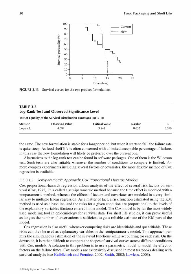
3.5.3.1.1 Illustration of Log-Rank Test to Compare FormulationsIn the following example, two groups of 21 cakes corresponding to the current and a new formu-lation were followed over time to assess their expected shelf life. Failure occurred as soon as mold appeared on a cake. Figure 3.13 shows the survival curve for both product formulations (the solid line is the current formulation; the dotted line is the new formulation).

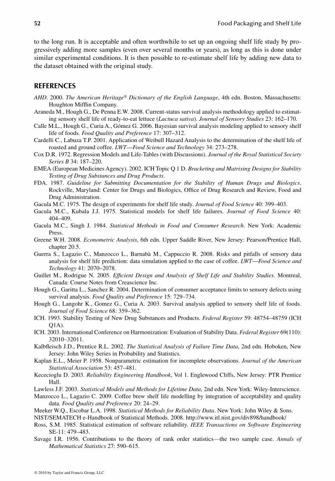
Table 3.3 shows the test statistic for the log-rank test and the associated p-value. As it is signi� -cant at the 5% level (p = 0.032), this suggests that the overall shape of the two survival curves is not

78445_C003.indd 4978445_C003.indd 49 10/16/2009 1:40:19 AM10/16/2009 1:40:19 AM



the same. The new formulation is stable for a longer period, but when it starts to fail, the failure rate is quite steep. As food shelf life is often concerned with a limited acceptable percentage of failure, in this case the new formulation will likely be preferred over the current one.

Alternatives to the log-rank test can be found in software packages. One of them is the Wilcoxon test. Such tests are also suitable whenever the number of conditions to compare is limited. For more complex experiments including several factors or covariates, the more I exible method of Cox regression is available.

3.5.3.1.2 Semiparametric Approach: Cox Proportional-Hazards ModelsCox proportional-hazards regression allows analysis of the effect of several risk factors on sur-vival (Cox, 1972). It is called a semiparametric method because the time effect is modeled with a nonparametric method, whereas the effects of factors and covariates are modeled in a very simi-lar way to multiple linear regression. As a matter of fact, a risk function estimated using the KM method is used as a baseline, and the risks for a given condition are proportional to the levels of the explanatory variables (factors) entered in the model. The Cox model is by far the most widely used modeling tool in epidemiology for survival data. For shelf life studies, it can prove useful as long as the number of observations is suf� cient to get a reliable estimate of the KM part of the model.

Cox regression is also useful whenever competing risks are identi� able and quanti� able. These risks can then be used as explanatory variables in the semiparametric model. This approach per-mits the simultaneous estimation of the survival functions while accounting for each risk. On the downside, it is rather dif� cult to compare the shapes of survival curves across different conditions with Cox models. A solution to this problem is to use a parametric model to model the effect of factors on the failure times. Cox models are extensively discussed in most textbooks dealing with survival analysis (see KalbI eisch and Prentice, 2002; Smith, 2002; Lawless, 2003).

TABLE 3.3Log-Rank Test and Observed Signifi cance Level

Test of Equality of the Survival Distribution Functions (DF = 1):

Statistic Observed Value Critical Value p-Value �

Log-rank 4.584 3.841 0.032 0.050

00

1020304050

Surv

ival

pro

babi

lity

(%)

60708090

100

5 10Time (days)

15 20 25

CurrentNew

FIGURE 3.13 Survival curves for the two product formulations.

78445_C003.indd 5078445_C003.indd 50 10/16/2009 1:40:19 AM10/16/2009 1:40:19 AM



3.5.3.1.3 Parametric Models: Regression with Life DataThe underlying principle in parametric regression for life data is quite simple: a parametric distri-bution is used to model the failure times, and a regression model is built to explain the failure time as a function of the different factors. It is possible to include censored observations in the analysis, and the interpretation of results is similar to that of multiple-regression model results. When there are few samples in the study, this is a more ef� cient way of analyzing the data than relying on a nonparametric method. However, all the issues discussed in the section on parametric distribution � tting also apply to this type of model. This implies that the most appropriate parametric distribu-tion must be selected and validated before interpreting any results from the model. Smith (2002) offers in-depth coverage of such models.

3.6 SUMMARY: BEST PRACTICES FOR SUCCESSFUL SHELF LIFE STUDIES

Shelf life data possess properties that make them different from other data collected in research and development. The two most important features are the non-normality of these data and the common occurrence of censored observations. Therefore, they cannot be analyzed using classical statistical tools such as ANOVA or linear regression. For simple experiments in which the shelf life of a prod-uct stored in well-de� ned conditions is tested, one can either use a nonparametric approach (the KM methodology) or � t a parametric distribution to the data. Whenever different conditions need to be compared, a variety of modeling tools generalizing the classical methods are available. These also share the speci� city of being based on either nonparametric or parametric models.

Nonparametric models are more I exible as far as assumptions are concerned and can be applied to the data even if the study has not ended. However, they do require more data than parametric models to provide precise estimates. Parametric methods also provide smooth curves instead of step functions.

As far as the design of shelf life studies is concerned, speci� c attention is also required. First of all, as shelf life studies are focused on the analysis of time-to-event data, an exact event de� nition is crucial for the success of the study. If failure might occur for several reasons (competing risks), this should be anticipated, recorded in the results, and properly handled in the analysis. In the same way, if censoring is likely to occur during the study (most often right- or interval-censoring), it should not be overlooked and should again be recorded in the results and taken care of in the data analysis. If the retained measurement involves destructive testing, the design must be adjusted according to the sources of variability in the study, and a two-step sampling procedure should be considered.

However, the design of shelf life studies also allows greater I exibility for several aspects than most other experimental situations. First, if the samples are not monitored in real time and time points must be selected to evaluate them, these time points do not need to be equally spaced and should be chosen to be more frequent at times of greater change. A second important feature is that shelf life designs can be easily adjusted or augmented at any moment to improve their performance. It is therefore a good idea to store additional samples and be prepared to make such adjustments.

Several additional aspects should not be overlooked when presenting study results. First, it is crucial to state clearly the scope of the study, especially the experimental conditions and how rep-resentative they are of the target real-life situation. Second, the two (often subjective) decisions concerning the exact de� nition of product failure (to record time-to-event data accurately) and the percentage of acceptable failures (to extract the single shelf life estimate from the survival curve) should be presented, along with a justi� cation of the choices that have been made. Third, when the � nal shelf life estimate is presented, it should be accompanied by a measure of uncertainty, typi-cally a con� dence interval. If a single value has to be given for practical reasons, it should be the lower bound of the con� dence interval rather than the estimate itself.

Finally, the presentation of results, especially in industrial applications, should contain sugges-tions of possible improvements for the estimates. It is rarely possible to have access to unlimited resources for a given study, but the I exibility concerning the experimental design actually extends

78445_C003.indd 5178445_C003.indd 51 10/16/2009 1:40:20 AM10/16/2009 1:40:20 AM



to the long run. It is acceptable and often worthwhile to set up an ongoing shelf life study by pro-gressively adding more samples (even over several months or years), as long as this is done under similar experimental conditions. It is then possible to re-estimate shelf life by adding new data to the dataset obtained with the original study.

REFERENCES

AHD. 2000. The American Heritage® Dictionary of the English Language, 4th edn. Boston, Massachusetts: Houghton MifI in Company.

Araneda M., Hough G., De Penna E.W. 2008. Current-status survival analysis methodology applied to estimat-ing sensory shelf life of ready-to-eat lettuce (Lactuca sativa). Journal of Sensory Studies 23: 162–170.

Calle M.L., Hough G., Curia A., Gómez G. 2006. Bayesian survival analysis modeling applied to sensory shelf life of foods. Food Quality and Preference 17: 307–312.

Cardelli C., Labuza T.P. 2001. Application of Weibull Hazard Analysis to the determination of the shelf life of roasted and ground coffee. LWT—Food Science and Technology 34: 273–278.

Cox D.R. 1972. Regression Models and Life-Tables (with Discussions). Journal of the Royal Statistical Society Series B 34: 187–220.

EMEA (European Medicines Agency). 2002. ICH Topic Q 1 D. Bracketing and Matrixing Designs for Stability Testing of Drug Substances and Drug Products.

FDA. 1987. Guideline for Submitting Documentation for the Stability of Human Drugs and Biologics. Rockville, Maryland: Center for Drugs and Biologics, Of� ce of Drug Research and Review, Food and Drug Administration.

Gacula M.C. 1975. The design of experiments for shelf life study. Journal of Food Science 40: 399–403.Gacula M.C., Kubala J.J. 1975. Statistical models for shelf life failures. Journal of Food Science 40:

404–409.Gacula M.C., Singh J. 1984. Statistical Methods in Food and Consumer Research. New York: Academic

Press.Greene W.H. 2008. Econometric Analysis, 6th edn. Upper Saddle River, New Jersey: Pearson/Prentice Hall,

chapter 20.5.Guerra S., Lagazio C., Manzocco L., Barnabà M., Cappuccio R. 2008. Risks and pitfalls of sensory data

analysis for shelf life prediction: data simulation applied to the case of coffee. LWT—Food Science and Technology 41: 2070–2078.

Guillet M., Rodrigue N. 2005. Ef+ cient Design and Analysis of Shelf Life and Stability Studies. Montreal, Canada: Course Notes from Creascience Inc.

Hough G., Garitta L., Sanchez R. 2004. Determination of consumer acceptance limits to sensory defects using survival analysis. Food Quality and Preference 15: 729–734.

Hough G., Langohr K., Gomez G., Curia A. 2003. Survival analysis applied to sensory shelf life of foods. Journal of Food Science 68: 359–362.

ICH. 1993. Stability Testing of New Drug Substances and Products. Federal Register 59: 48754–48759 (ICH Q1A).

ICH. 2003. International Conference on Harmonization: Evaluation of Stability Data. Federal Register 69(110): 32010–32011.

KalbI eisch J.D., Prentice R.L. 2002. The Statistical Analysis of Failure Time Data, 2nd edn. Hoboken, New Jersey: John Wiley Series in Probability and Statistics.

Kaplan E.L., Meier P. 1958. Nonparametric estimation for incomplete observations. Journal of the American Statistical Association 53: 457–481.

Kececioglu D. 2003. Reliability Engineering Handbook, Vol 1. Englewood Cliffs, New Jersey: PTR Prentice Hall.

Lawless J.F. 2003. Statistical Models and Methods for Lifetime Data, 2nd edn. New York: Wiley-Interscience.Manzocco L., Lagazio C. 2009. Coffee brew shelf life modelling by integration of acceptability and quality

data. Food Quality and Preference 20: 24–29.Meeker W.Q., Escobar L.A. 1998. Statistical Methods for Reliability Data. New York: John Wiley & Sons.NIST/SEMATECH e-Handbook of Statistical Methods. 2008. http://www.itl.nist.gov/div898/handbook/Ross, S.M. 1985. Statistical estimation of software reliability. IEEE Transactions on Software Engineering

SE-11: 479–483.Savage I.R. 1956. Contributions to the theory of rank order statistics—the two sample case. Annals of

Mathematical Statistics 27: 590–615.

78445_C003.indd 5278445_C003.indd 52 10/16/2009 1:40:20 AM10/16/2009 1:40:20 AM



Schmidt K., Bouma J. 1992. Estimating shelf life of cottage cheese using hazard analysis. Journal of Dairy Science 75: 2922–2927.

Simon M., Hansen A.P. 2001. Effect of various dairy packaging materials on the shelf life and I avor of ultra-pasteurized milk. Journal of Dairy Science 84: 784–791.

Smith P.J. 2002. Analysis of Failure and Survival Data. Boca Raton, Florida: CRC Press.Stephens M.A. 1974. EDF statistics for goodness of � t and some comparisons. Journal of the American

Statistical Association 69: 730–737.Yamani M.I., Abu-Jaber M.M. 1994. Yeast I ora of labneh produced in bag straining of cow milk set yogurt.

Journal of Dairy Science 77: 2558–3564.

78445_C003.indd 5378445_C003.indd 53 10/16/2009 1:40:20 AM10/16/2009 1:40:20 AM


3 Shelf Life Testing Methodology and Data...

Documents

Transcript of 3 Shelf Life Testing Methodology and Data...