3 regression review - The University of Chicago · • in a linear regression the marginal effect...

Copyright © 2017 by Luc Anselin, All Rights Reserved

Luc Anselin

Spatial Regression3. Review - OLS and 2SLS

http://spatial.uchicago.edu


• OLS estimation (recap)

• non-spatial regression diagnostics

• endogeneity - IV and 2SLS


OLS Estimation (recap)


• Linear Regression - Notation

• linear relationship between a dependent variable yi (at location i) and a set of explanatory variables xih, for h = 1, ..., k subject to random error

• yi = Σh xih βh + ei

• ei is random error term, with E[ ei ] = 0, i.e., no systematic error


• Linear Regression - Notation (continued)

• in matrix notation, a n times 1 column vector y and a n times k vector X, with a k times 1 coefficient vector β and a n times 1 random error vector e

• y = Xβ + e

• E[ e ] = 0


• Conditional Expectation

• under a set of regularity conditions (to follow) the conditional expectation of y given X is linear in X

• E[ y | X ] = E [Xβ | X ] + E[ e | X ] = Xβ + 0

• in other words, what would y be on average if we knew X


• Marginal Effect

• the effect of a change in X on y

• in a linear regression the marginal effect equals the regression coefficient (this is not the case in a nonlinear regression)

• E [ y | ∆X ] = ∆X β


• Selected Regularity Conditions

• X non-stochastic (or if stochastic, with bounds on second moment) - the only randomness follows from the dependent variable y, any randomness in X is inconsequential

• error term independent identically distributed (i.i.d), i.e., Var [ei] = σ2 or E[ee’] = σ2I = spherical error term

• xi and ei uncorrelated for all i, i.e., signal (X) and noise (e) are not related


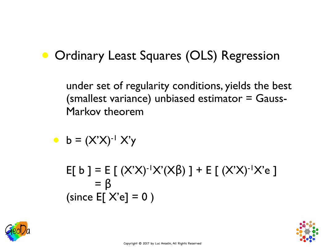
• Ordinary Least Squares (OLS) Regression

• under set of regularity conditions, yields the best (smallest variance) unbiased estimator = Gauss-Markov theorem

• b = (X’X)-1 X’y

• E[ b ] = E [ (X’X)-1X’(Xβ) ] + E [ (X’X)-1X’e ] = β(since E[ X’e] = 0 )


• OLS - Inference

• with non-spherical errors

• var(b) = s2 (X’X)-1

• s2 = e’e / n - k

• an unbiased estimator of error variance

• use in t-tests (with assumption of normality)


• Predicted Value

• value of yi given xi using the estimates b

• yip = Σh xih bh

• Residual

• difference between observed and predicted

• ui = yi - yip

• for regression with constant term avg[ui] = 0

• residual is NOT the same as the error term (ei)


• General Covariance Structure

• y = Xβ + e, E[ee’] = Ω

• both heteroskedasticity and autocorrelation

• Var[βOLS] = (1/n)(1/n X’X)-1(1/n X’ΩX)(1/n X’X)-1

• develop estimator for (1/n)X’ΩX (k by k) but NOT an estimator for Ω (n by n)

• example: White (sandwich) standard errors


Non-spatial Regression Diagnostics


Visual Diagnostics


• Predicted Value Map

• shows spatial distribution of model prediction

• a form of smoothing, i.e., what the model suggests y should be, given the X at each location


Predicted Value map - 1990 county homicide rates(standard deviational map)


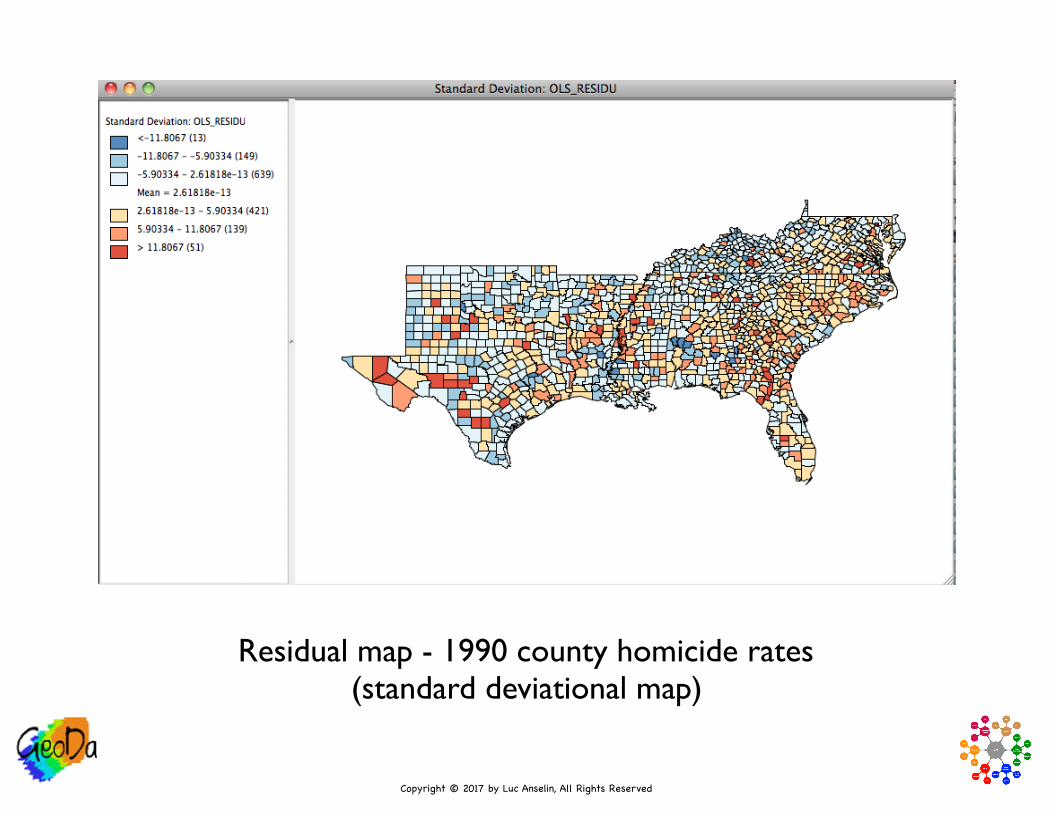
• Residual Map

• high values (red) = model under-predicts (y > yp)

• low values (blue) = model over-predicts (y < yp)

• note extremes = poor fit of model

• note spatial patterns, but visual inspection can be misleading

• need for formal diagnostics


Residual map - 1990 county homicide rates(standard deviational map)


• Diagnostic Plots

• use scatter plot function

• plot residuals (y-axis) vs. predicted values (x-axis) as a visual diagnostic for heteroskedasticity

• pattern should be more or less within the same range

• “fan” or “flares” suggest heteroskedasticity, i.e., non-constant error variance


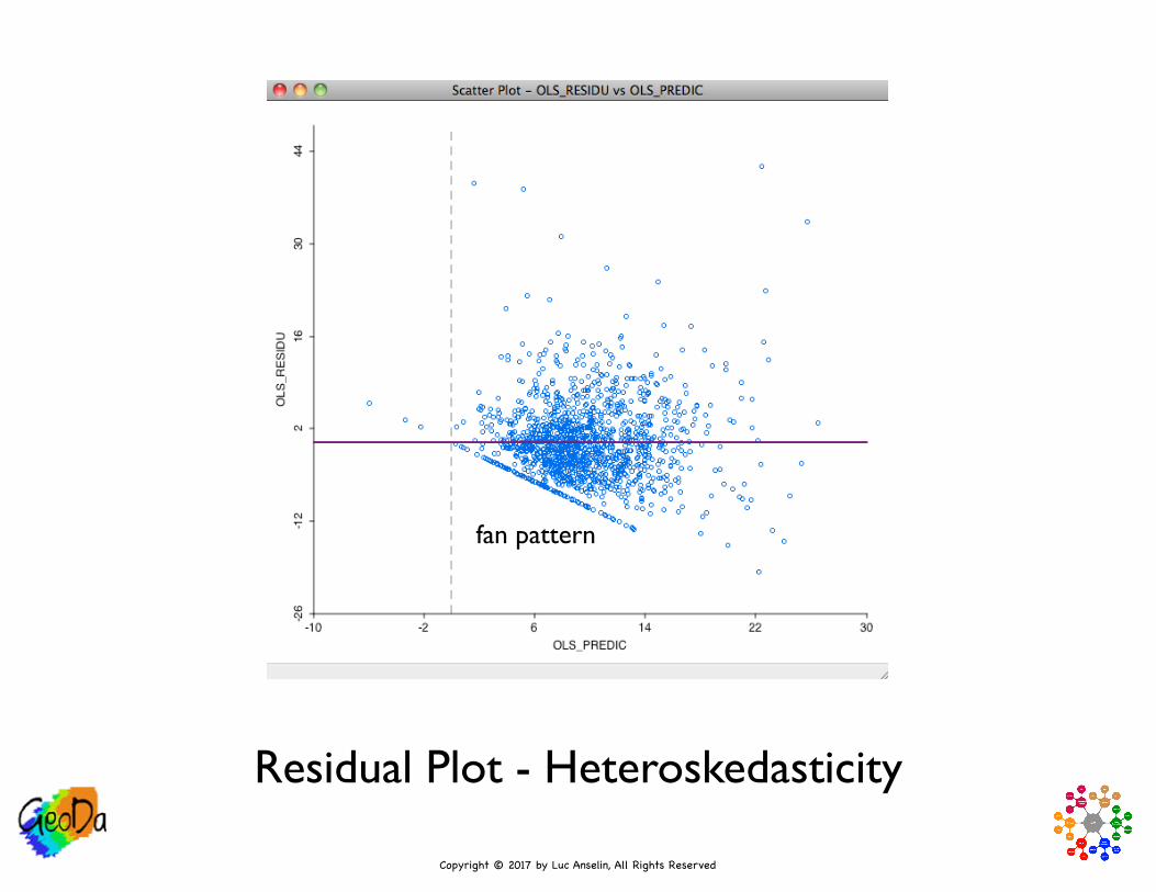
Residual Plot - Heteroskedasticity

fan pattern


• Caution

• visual inspection of plots and maps can be misleading

• use plots and maps to suggest additional variables for model

• no substitute for formal specification diagnostics


Specification Tests


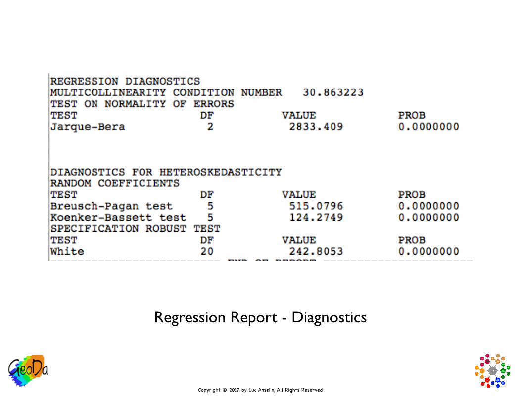
Regression Report - Diagnostics


• Multicollinearity

• condition number

• based on eigenvalues of X’X

• “classic” rule of thumb = values > 30 suggest a problem

• in practice, not taken too literally

• in example, slightly over 30


• Normality

• crucial assumption for exact inference

• in practice, less crucial, since asymptotics (large sample theory) yield similar properties

• Bera-Jarque(1981) test is based on third moment (skewness - asymmetry) and fourth moment (kurtosis - thick tails) of residuals

• distributed as χ2 with two degrees of freedom

• in example: 2833, thus highly non-normal


• Random Coefficients

• a special form of heteroskedasticity

• measure of fit of regression of squared residuals on squared explanatory variables

• Breusch-Pagan (1979) test and a robustified version (for non-normality) Koenker-Bassett (1982) test

• in example: both reject null very strongly


• Heteroskedasticity

• White (1980) test against heteroskedasticity of unknown form

• measure of fit of regression of squared residuals on a polynomial in the explanatory variables

• robust to many forms of misspecification

• in example: rejects the null soundly


• Caveats

• in large data sets (as in the south example), lack of normality is not a real problem

• heteroskedasticity is hard to distinguish from spatial autocorrelation (and vice versa)

• many types of misspecification (missing variables, nonlinearity) may lead to the rejection of a given null hypothesis, even when unrelated to that null hypothesis


EndogeneityIV and 2SLS


Simultaneous Equation Bias


• Regularity Conditions

• E[ xi | ei ] = 0 implies E[e] = 0 and E[X’e] = 0 establishes unbiasedness

• weaker Cov[X’e] =0 for consistency

• plim (1/n) X’e = 0


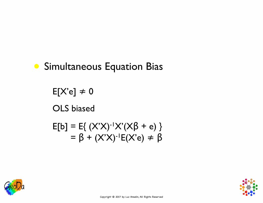
• Simultaneous Equation Bias

• E[X’e] ≠ 0

• OLS biased

• E[b] = E{ (X’X)-1X’(Xβ + e) } = β + (X’X)-1E(X’e) ≠ β


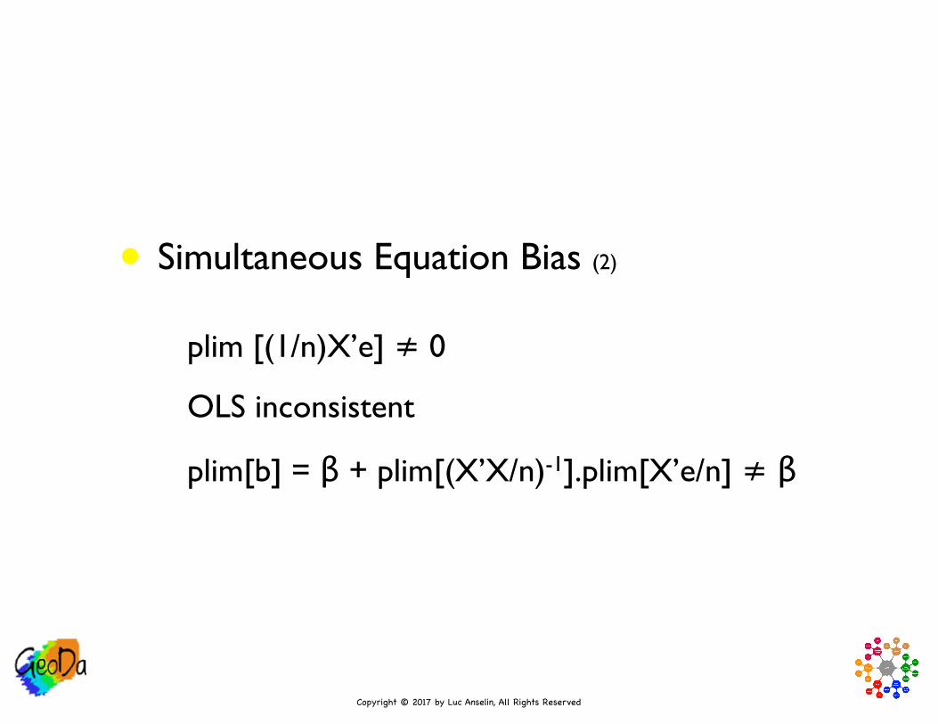
• Simultaneous Equation Bias (2)

• plim [(1/n)X’e] ≠ 0

• OLS inconsistent

• plim[b] = β + plim[(X’X/n)-1].plim[X’e/n] ≠ β


Instruments


• General Model

• y = Zθ + e

• some zki correlated with ei

• two sources of variation: error and Z


• Instruments

• new variable q

• uncorrelated with errors E[ ei | qi ] = 0

• correlated with original Z


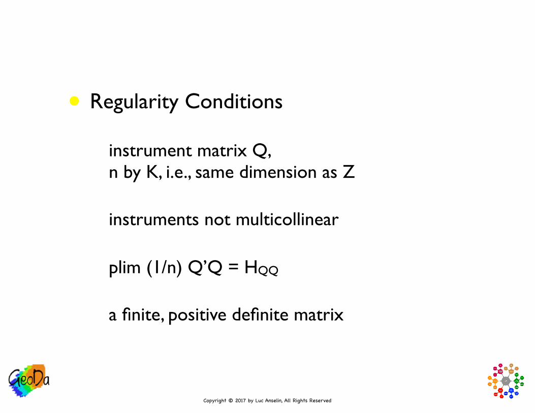
• Regularity Conditions

• instrument matrix Q, n by K, i.e., same dimension as Z

• instruments not multicollinear

• plim (1/n) Q’Q = HQQ

• a finite, positive definite matrix


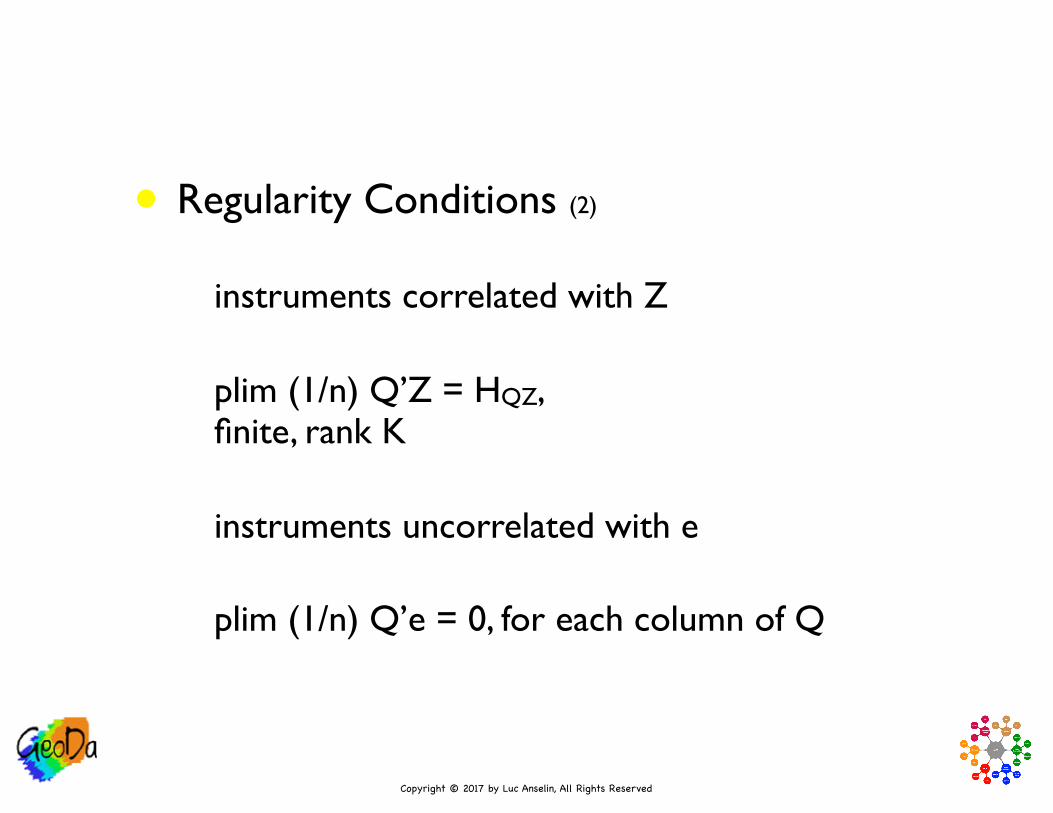
• Regularity Conditions (2)

• instruments correlated with Z

• plim (1/n) Q’Z = HQZ, finite, rank K

• instruments uncorrelated with e

• plim (1/n) Q’e = 0, for each column of Q


IV Estimator


• Estimator

• θIV = (Q’Z)-1Q’y

• consistency

• θIV = (Q’Z)-1Q’(Zθ + e)

• θIV = = θ + (Q’Z)-1Q’e

• plim(θIV) = θ + plim(Q’Z/n)-1plim(Q’e/n) = θ + HQZ-1.0 = θ


• Limiting Distribution

• √n (θIV - θ) = (Q’Z/n)-1(Q’e/√n)

• limiting distribution depends on Q’e/√n

• requires central limit theorem to establish asymptotic normality

• requires law of large numbers to establish consistency of asymptotic variance


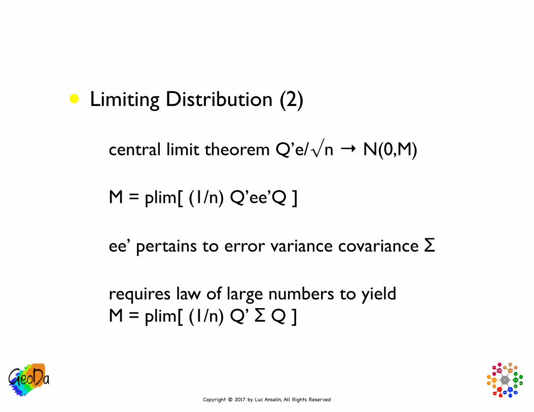
• Limiting Distribution (2)

• central limit theorem Q’e/√n → N(0,M)

• M = plim[ (1/n) Q’ee’Q ]

• ee’ pertains to error variance covariance Σ

• requires law of large numbers to yieldM = plim[ (1/n) Q’ Σ Q ]


• Asymptotic Variance

• variance of √n (θIV - θ) is variance of (Q’Z/n)-1(Q’e/√n), a constant (matrix) times a random variable (vector)

• plim(Q’Z/n)-1. plim(Q’ Σ Q /n].plim(Z’Q/n)-1 = HQZ-1MHZQ-1


• Asymptotic Distribution

• √n (θIV - θ) → N(0, HQZ-1MHZQ-1)

• θIV → N(θ, HQZ-1MHZQ-1/n)

• Var[θIV] = (1/n)(Q’Z/n)-1(Q’ΣQ/n)(Z’Q/n)-1

• note: all n terms cancel out, s.t., variance can be estimated asVar[θIV] = (Q’Z)-1(Q’ΣQ)(Z’Q)-1


2SLS Estimator


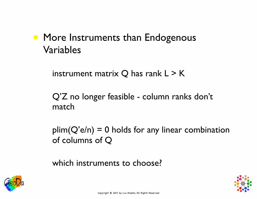
• More Instruments than Endogenous Variables

• instrument matrix Q has rank L > K

• Q’Z no longer feasible - column ranks don’t match

• plim(Q’e/n) = 0 holds for any linear combination of columns of Q

• which instruments to choose?


• Projection Matrix

• could pick any K columns from Q

• optimal choice is combination of columns of Q closest to Z

• Zp = Q(Q’Q)-1Q’Z predicted values of least squares regression (projection) of Q onto columns of Z yields K “instruments”

• PQ = Q(Q’Q)-1Q’ is the projection matrix


• 2SLS Estimation

• use Zp as matrix of instruments

• θ2SLS = (Zp’Z)-1Zp’y

• Zp’Z = Zp’Zp same as OLS of y on Zp

• θ2SLS = (Zp’Zp)-1Zp’y


• Two Stages

• stage one: OLS of Q on each of the columns of Z yields predicted values Zp

• stage two: OLS of y on Zp

• proper residuals are y - Zθ2SLS NOT y - Zpθ2SLS

• θ2SLS = [Z’Q(Q’Q)-1Q’Z]-1Z’Q(Q’Q)-1Q’y


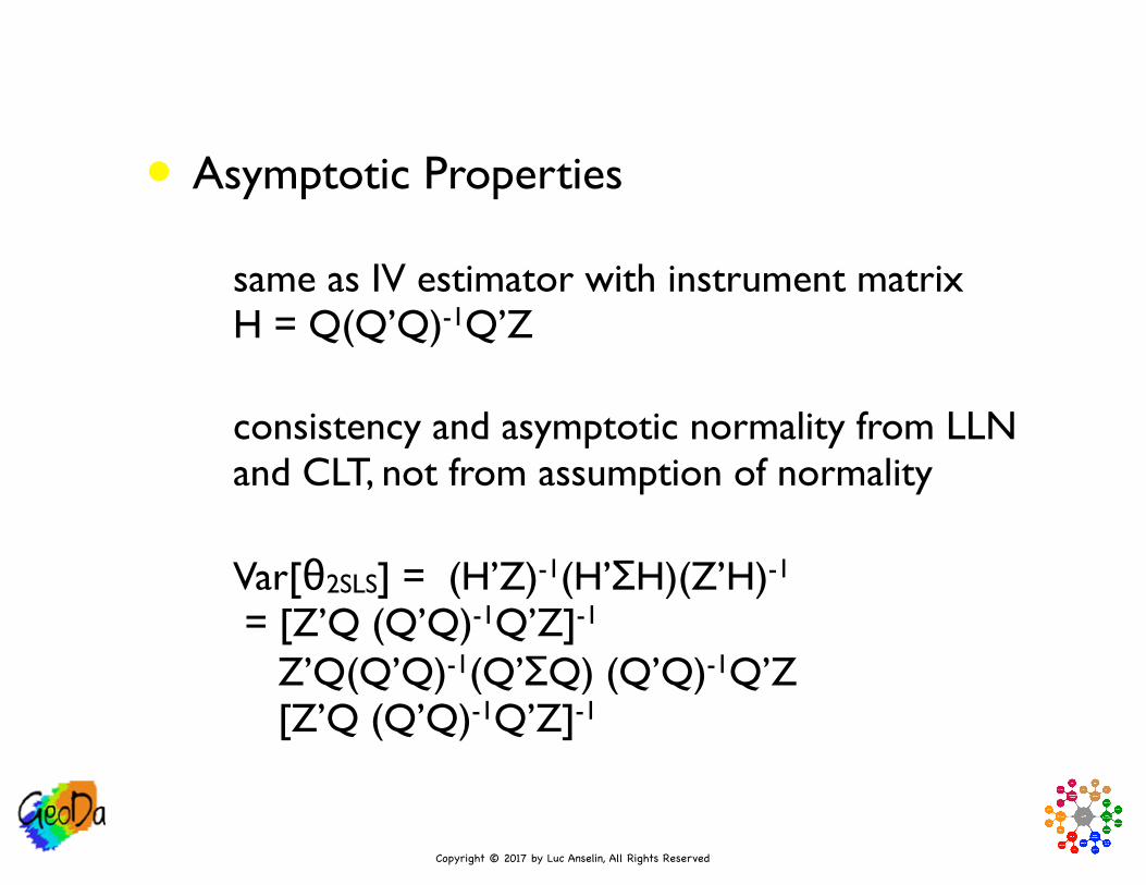
• Asymptotic Properties

• same as IV estimator with instrument matrix H = Q(Q’Q)-1Q’Z

• consistency and asymptotic normality from LLN and CLT, not from assumption of normality

• Var[θ2SLS] = (H’Z)-1(H’ΣH)(Z’H)-1 = [Z’Q (Q’Q)-1Q’Z]-1 Z’Q(Q’Q)-1(Q’ΣQ) (Q’Q)-1Q’Z [Z’Q (Q’Q)-1Q’Z]-1


Illustration


• Homicide Rate Regression - south.dbf

• HR90: county homicide rate

• RD90: resource deprivation

• PS90: population structure component

• MA90: median age

• UE90: unemployment rate


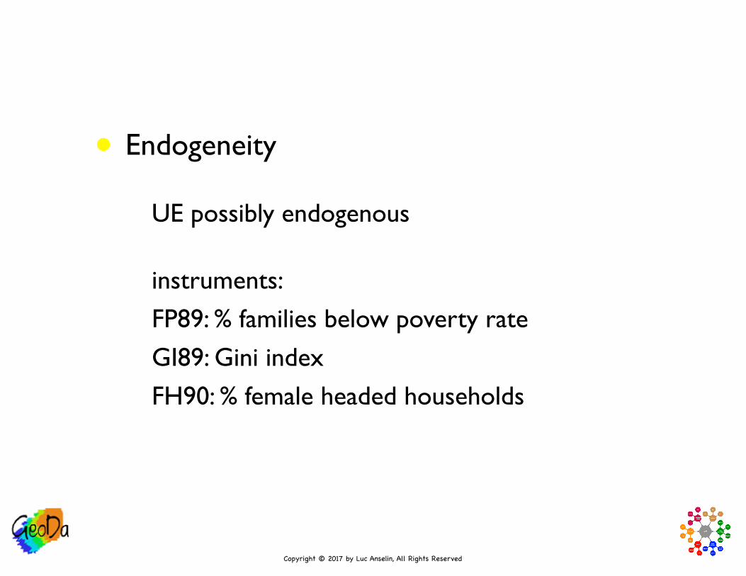
• Endogeneity

• UE possibly endogenous

• instruments: FP89: % families below poverty rate GI89: Gini index FH90: % female headed households


• Ordinary Least Squares Regression

• HR90 on RD90, PS90, MA90 and UE90

• for reference purposes only

• if UE90 is indeed endogenous, then the OLS estimates will be biased


OLS Results


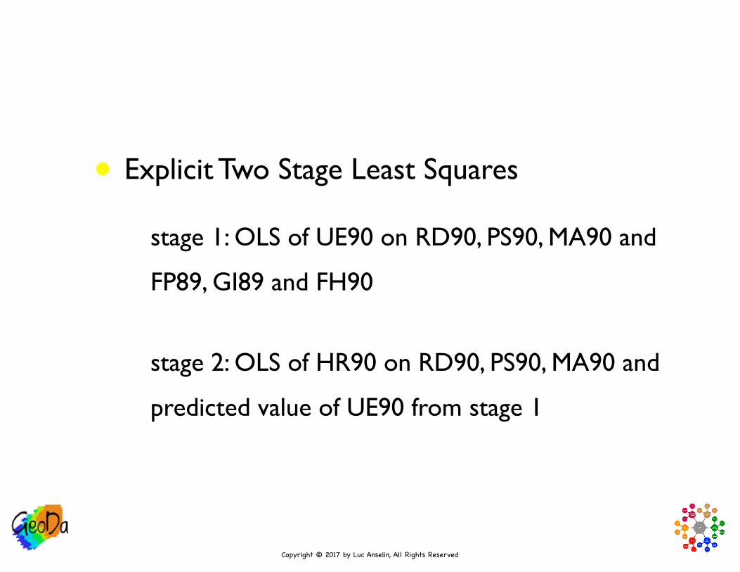
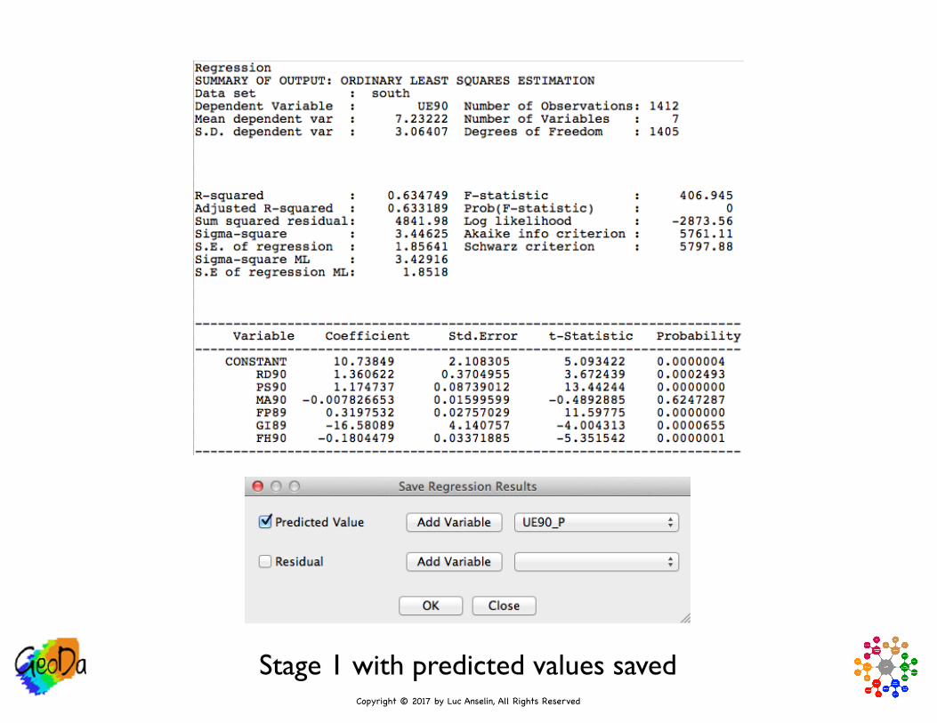
• Explicit Two Stage Least Squares

• stage 1: OLS of UE90 on RD90, PS90, MA90 and

FP89, GI89 and FH90

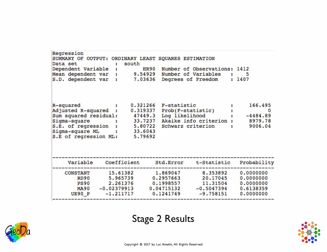
• stage 2: OLS of HR90 on RD90, PS90, MA90 and

predicted value of UE90 from stage 1


Stage 1 with predicted values saved


Stage 2 Results


• Proper 2SLS

• same coefficient estimates as two stage approach

• correct residuals

• different error variance

• different coefficient variance estimates and t statistics


2SLS variable selection in GeoDaSpace


2SLS GeoDaSpace Results


Var OLS Two Stage 2SLS

Constant 10.59 15.61 15.61

RD90 4.56 5.97 5.97

PS90 2.13 2.26 2.26

MA90 -0.003 -0.02 -0.02

UE90 -0.51 -1.21 -1.21

Comparison: Coefficient Estimates


Var OLS Two Stage 2SLS

Constant 1.74 1.87 1.96

RD90 0.22 0.3 0.31

PS90 0.2 0.2 0.21

MA90 0.048 0.047 0.049

UE90 0.07 0.12 0.13

Comparison: Coefficient Standard Errors

3 regression review - The University of Chicago · • in a linear regression the marginal effect...

Documents

Transcript of 3 regression review - The University of Chicago · • in a linear regression the marginal effect...