Combining these two partial derivatives leads to:

[A.2]

By setting 2F(m) − 1 = 0, we solve for the value of F(m) = 1/2, that is,the median, to satisfy the minimization problem.

Repeating the above argument for quantiles, the partial derivative forquantiles corresponding to Equation A.2 is:

[A.3]

We set the partial derivative F(q) − p = 0 and solve for the value ofF(q) = p that satisfies the minimization problem.

3. QUANTILE-REGRESSION MODEL AND ESTIMATION

The quantile functions described in Chapter 2 are adequate for describ-ing and comparing univariate distributions. However, when we model therelationship between a response variable and a number of independentvariables, it becomes necessary to introduce a regression-type model for the quantile function, the quantile-regression model (QRM). Given a set ofcovariates, the linear-regression model (LRM) specifies the conditional-mean function whereas the QRM specifies the conditional-quantile func-tion. Using the LRM as a point of reference, this chapter introduces theQRM and its estimation. It makes comparisons between the basic modelsetup for the LRM and that for the QRM, a least-squares estimation forthe LRM and an analogous estimation approach for the QRM, and theproperties of the two types of models. We illustrate our basic points usingempirical examples from analyses of household income.1

Linear-Regression Modeling and Its Shortcomings

The LRM is a standard statistical method widely used in social-scienceresearch, but it focuses on modeling the conditional mean of a responsevariable without accounting for the full conditional distributional propertiesof the response variable. In contrast, the QRM facilitates analysis of the full

∂

∂qE[dp(Y, q)] = (1 − p)F(q) − p(1 − F(q)) = F(q) − p.

∂

∂m

∫ +∞

−∞|y − m|f (y)dy = F(m) − (1 − F(m)) = 2F(m) − 1.

22

03-Hao.qxd 3/13/2007 5:24 PM Page 22

23

conditional distributional properties of the response variable. The QRM andLRM are similar in certain respects, as both models deal with a continuousresponse variable that is linear in unknown parameters, but the QRM andLRM model different quantities and rely on different assumptions abouterror terms. To better understand these similarities and differences, we layout the LRM as a starting point, and then introduce the QRM. To aid theexplication, we focus on the single covariate case. While extending to morethan one covariate necessarily introduces additional complexity, the ideasremain essentially the same.

Let y be a continuous response variable depending on x. In our empiricalexample, the dependent variable is household income. For x, we use aninterval variable, ED (the household head’s years of schooling), or alterna-tively a dummy variable, BLACK (the head’s race, 1 for black and 0 forwhite). We consider data consisting of pairs (xi ,yi) for i = 1, . . . , n basedon a sample of micro units (households in our example).

By LRM, we mean the standard linear-regression model

yi = β0 + β1x i + ε i , [3.1]

where εi is identically, independently, and normally distributed with meanzero and unknown variance σ 2. As a consequence of the mean zeroassumption, we see that the function β 0 + β 1x being fitted to the data corre-sponds to the conditional mean of y given x (denoted by E[ y ⎢x]), which isinterpreted as the average in the population of y values corresponding to afixed value of the covariate x.

For example, when we fit the linear-regression Equation 3.1 usingyears of schooling as the covariate, we obtain the prediction equationy = –23127 + 5633ED, so that plugging in selected numbers of years of schooling leads to the following values of conditional means forincome.

ED 9 12 16E ( y | ED) $27,570 $44,469 $67,001

Assuming a perfect fit, we would interpret these values as the averageincome for people with a given number of years of schooling. For example,the average income for people with nine years of schooling is $27,570.

Analogously, when we take the covariate to be BLACK, the fitted regres-sion equation takes the form y = 53466 – 18268BLACK, and plugging in thevalues of this covariate yields the following values.

03-Hao.qxd 3/13/2007 5:24 PM Page 23

Again assuming the fitted model to be a reflection of what happens at thepopulation level, we would interpret these values as averages in subpopulations,for example, the average income is $53,466 for whites and $35,198 for blacks.

Thus, we see that a fundamental aspect of linear-regression models isthat they attempt to describe how the location of the conditional distribu-tion behaves by utilizing the mean of a distribution to represent its centraltendency. Another key feature of the LRM is that it invokes a homoscedas-ticity assumption; that is, the conditional variance, Var (y|x), is assumed tobe a constant σ 2 for all values of the covariate. When homoscedasticityfails, it is possible to modify LRM by allowing for simultaneous modelingof the conditional mean and the conditional scale. For example, one canmodify the model in Equation 3.1 to allow for modeling the conditionalscale: yi = β0 + β1x i + e γε i, where γ is an additional unknown parameterand we can write Var (y|x) = σ 2e γ.

Thus, utilizing LRM reveals important aspects of the relationshipbetween covariates and a response variable, and can be adapted to performthe task of modeling what is arguably the most important form of shapechange for a conditional distribution: scale change. However, the estimationof conditional scale is not always readily available in statistical software.In addition, linear-regression models impose significant constraints on themodeler, and it is challenging to use LRM to model more complex condi-tional shape shifts.

To illustrate the kind of shape shift that is difficult to model using LRM,imagine a somewhat extreme situation in which, for some population ofinterest, we have a response variable y and a covariate x with the propertythat the conditional distribution of y has the probability density of the formshown in Figure 3.1 for each given value of x = 1,2,3. The three probabil-ity density functions in this figure have the same mean and standard devia-tion. Since the conditional mean and scale for the response variable y donot vary with x, there is no information to be gleaned by fitting a linear-regression model to samples from these populations. In order to understandhow the covariate affects the response variable, a new tool is required.Quantile regression is an appropriate tool for accomplishing this task.

A third distinctive feature of the LRM is its normality assumption.Because the LRM ensures that the ordinary least squares provide the bestpossible fit for the data, we use the LRM without making the normalityassumption for purely descriptive purposes. However, in social-scienceresearch, the LRM is used primarily to test whether an explanatory variable

24

BLACK 0 1E ( y | BLACK) $53,466 $35,198

03-Hao.qxd 3/13/2007 5:24 PM Page 24

significantly affects the dependent variable. Hypothesis testing goes beyondparameter estimation and requires determination of the sampling variabil-ity of estimators. Calculated p-values rely on the normality assumption oron large-sample approximation. Violation of these conditions may causebiases in p-values, thus leading to invalid hypothesis testing.

A related assumption made in the LRM is that the regression model usedis appropriate for all data, which we call the one-model assumption.Outliers (cases that do not follow the relationship for the majority of thedata) in the LRM tend to have undue influence on the fitted regression line.The usual practice used in the LRM is to identify outliers and eliminatethem. Both the notion of outliers and the practice of eliminating outliersundermine much social-science research, particularly studies on socialstratification and inequality, as outliers and their relative positions to thoseof the majority are important aspects of inquiry. In terms of modeling, onewould simultaneously need to model the relationship for the majority casesand for the outlier cases, a task the LRM cannot accomplish.

25

0.5 1.0 1.5

1.5

1.0

0.5

0.0

2.0 2.5

Y

x = 3

x = 1x = 2

Figure 3.1 Conditional Distributions With the Same Mean and StandardDeviation but Different Skewness

03-Hao.qxd 3/13/2007 8:28 PM Page 25

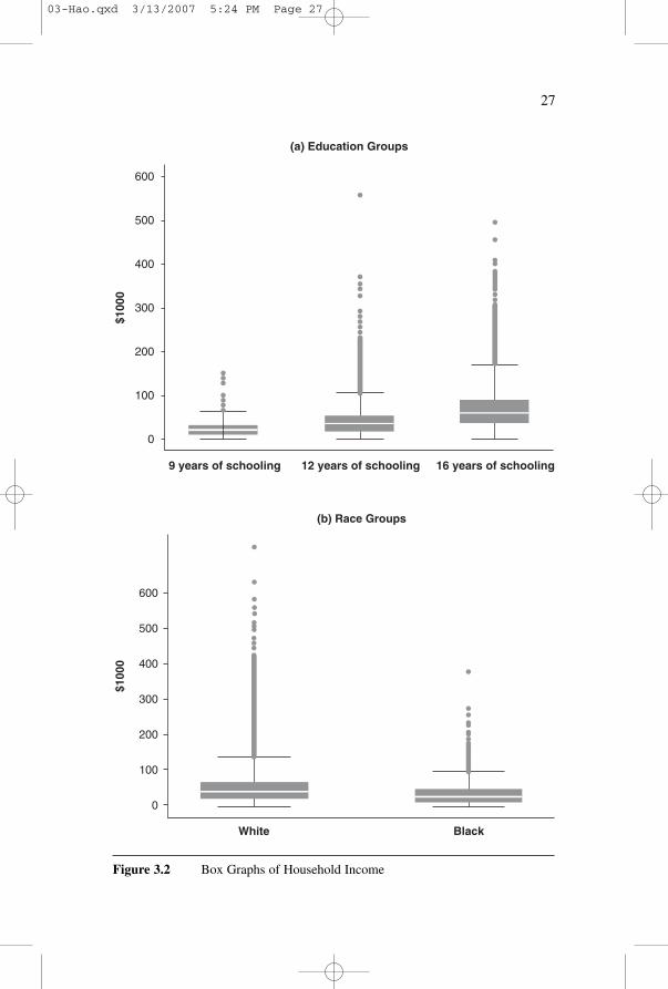
All of the features just mentioned are exemplified in our householdincome data: the inadequacy of the conditional mean from a distributionalpoint of view and violations of the homoscedasticity assumption, the nor-mality assumption, and the one-model assumption. Figure 3.2 shows thedistributions of income by education groups and racial groups. The locationshifts among the three education groups and between blacks and whites areobvious, and their shape shifts are substantial. Therefore, the conditionalmean from the LRM fails to capture the shape shifts caused by changes inthe covariate (education or race). In addition, since the spreads differ sub-stantially among the education groups and between the two racial groups,the homoscedasticity assumption is violated, and the standard errors arenot estimated precisely. All box graphs in Figure 3.2 are right-skewed.Conditional-mean and conditional-scale models are not able to detect thesekinds of shape changes.

By examining residual plots, we have identified seven outliers, includingthree cases with 18 years of schooling having an income of more than$505,215 and four cases with 20 years of schooling having an income ofmore than $471,572. When we add a dummy variable indicating member-ship in this outlier class to the regression model of income on education, wefind that these cases contribute an additional $483,544 to the intercept.

These results show that the LRM approach can be inadequate for a vari-ety of reasons, including heteroscedasticity and outlier assumptions and thefailure to detect multiple forms of shape shifts. These inadequacies are notrestricted to the study of household income but also appear when othermeasures are considered. Therefore, it is desirable to have an alternativeapproach that is built to handle heteroscedasticity and outliers and detectvarious forms of shape changes.

As pointed out above, the conditional mean fails to identify shape shifts.The conditional-mean models also do not always correctly model centrallocation shifts if the response distribution is asymmetric. For a symmetricdistribution, the mean and median coincide, but the mean of a skewed dis-tribution is no longer the same as the median (the .5th quantile). Table 3.1shows a set of brief statistics describing the household income distribution.The right-skewness of the distribution makes the mean considerably largerthan the median for both the total sample and for education and racialgroups (see the first two rows of Table 3.1). When the mean and the medianof a distribution do not coincide, the median may be more appropriate tocapture the central tendency of the distribution. The location shifts amongthe three education groups and between blacks and whites are considerablysmaller when we examine the median rather than the mean. This differenceraises concerns about using the conditional mean as an appropriate measurefor modeling the location shift of asymmetric distributions.

26

03-Hao.qxd 3/13/2007 5:24 PM Page 26

27

600

(a) Education Groups

500

400

300

200

100

0

$100

0

9 years of schooling 12 years of schooling 16 years of schooling

600

500

400

300

200

100

0

$100

0

White Black

(b) Race Groups

Figure 3.2 Box Graphs of Household Income

03-Hao.qxd 3/13/2007 5:24 PM Page 27

28

TAB

LE

3.1

Hou

seho

ld I

ncom

e D

istr

ibut

ion:

Tota

l,E

duca

tion

Gro

ups,

and

Rac

ial G

roup

s

Tota

lE

D =

9E

D =

12E

D =

16W

HIT

EB

LA

CK

Mea

n50

,334

27,8

4140

,233

71,8

3353

,466

35,1

98

Qua

ntil

eM

edia

n (.

50th

Qua

ntile

)39

,165

22,1

4632

,803

60,5

4541

,997

26,7

63.1

0th

Qua

ntile

11,0

228,

001

10,5

1021

,654

12,4

866,

837

.25t

h Q

uant

ile20

,940

12,3

2918

,730

36,8

0223

,198

13,4

12.7

5th

Qua

ntile

65,7

9336

,850

53,0

7590

,448

69,6

8047

,798

.90t

h Q

uant

ile98

,313

54,3

7077

,506

130,

981

102,

981

73,0

30

Qua

ntil

e-B

ased

Sca

le(Q

.75−

Q.2

5)44

,853

24,5

2134

,344

53,6

4646

,482

34,3

86(Q

.90−

Q.1

0)87

,291

46,3

6966

,996

109,

327

90,4

9566

,193

Qua

ntil

e-B

ased

Ske

wne

ss(Q

.75−

Q.5

0) −1

(Q.5

0−Q

.25)

.46

.50

.44

.26

.47

.58

(Q.9

0−Q

.50)

−1(Q

.50−

Q.1

0)1.

101.

281.

01.8

11.

071.

32

03-Hao.qxd 3/13/2007 5:24 PM Page 28

Conditional-Median and Quantile-Regression Models

With a skewed distribution, the median may become the more appropriatemeasure of central tendency; therefore, conditional-median regression,rather than conditional-mean regression, should be considered for thepurpose of modeling location shifts. Conditional-median regression wasproposed by Boscovich in the mid-18th century and was subsequentlyinvestigated by Laplace and Edgeworth. The median-regression modeladdresses the problematic conditional-mean estimates of the LRM. Medianregression estimates the effect of a covariate on the conditional median, soit represents the central location even when the distribution is skewed.

To model both location shifts and shape shifts, Koenker and Bassett (1978)proposed a more general form than the median-regression model, the quan-tile-regression model (QRM). The QRM estimates the potential differentialeffect of a covariate on various quantiles in the conditional distribution, forexample, a sequence of 19 equally distanced quantiles from the .05th quan-tile to the .95th quantile. With the median and the off-median quantiles, these19 fitted regression lines capture the location shift (the line for the median),as well as scale and more complex shape shifts (the lines for off-medianquantiles). In this way, the QRM estimates the differential effect of a covari-ate on the full distribution and accommodates heteroscedasticity.

Following Koenker and Bassett (1978), the QRM corresponding to theLRM in Equation 3.1 can be expressed as:

yi = β (p)0 + β (p)

1 xi + ε (p)i , [3.2]

where 0 < p < 1 indicates the proportion of the population havingscores below the quantile at p. Recall that for LRM, the conditional meanof yi given x i is E(yi|xi ) = β0 + β 1x i, and this is equivalent to requiringthat the error term ε i have zero expectation. In contrast, for the corre-sponding QRM, we specify that the pth conditional quantile given xi isQ (p)( yi|xi) = β (p)

0 + β (p)1 xi. Thus, the conditional pth quantile is determined

by the quantile-specific parameters, β (p)0 and β (p)

1 , and a specific value of thecovariate xi. As for the LRM, the QRM can be formulated equivalently witha statement about the error terms εi. Since the term β (p)

0 +β (p)1 x i is a constant,

we have Q (p)( yi|xi) = β (p)0 + β (p)

1 xi + Q(p)(εi ) = β (p)0 + β (p)

1 xi, so an equivalentformulation of QRM requires that the pth quantile of the error termbe zero.

It is important to note that for different values of the quantile p ofinterest, the error terms ε ( p)

i for fixed i are related. In fact, replacingp by q in Equation 3.2 gives yi = β (q)

0 + β (q)1 x i + ε (q)

i , which leads toε (p)

i – ε (q)i = (β (q)

0 – β (p)0 ) + xi( β (q)

1 – β (p)1 ), so that the two error terms differ by

29

03-Hao.qxd 3/13/2007 5:24 PM Page 29

a constant given x i. In other words, the distributions of ε (p)i and ε (q)

i are shiftsof one another. An important special case of QRM to consider is one inwhich the ε (p)

i for i = 1, . . . , n are independent and identically distributed;we refer to this as the i.i.d. case. In this situation, the qth quantile of ε (p)

i isa constant cp,q depending on p and q and not on i. Using Equation 3.2, wecan express the qth conditional-quantile function as Q(q)( yi|xi ) =Q(p)( yi|xi ) + cp,q.

2 We conclude that in the i.i.d. case, the conditional-quan-tile functions are simple shifts of one another, with the slopes β 1

(p) taking acommon value β1. In other words, the i.i.d. assumption says that there areno shape shifts in the response variable.

Equation 3.2 dictates that unlike the LRM in Equation 3.1, whichhas only one conditional mean expressed by one equation, the QRM canhave numerous conditional quantiles. Thus, numerous equations can beexpressed in the form of Equation 3.2.3 For example, if the QRM specifies19 quantiles, the 19 equations yield 19 coefficients for x i , one at each of the19 conditional quantiles ( β 1

.05, β 1.10, . . . , β 1

.95). The quantiles do not have tobe equidistant, but in practice, having them at equal intervals makes themeasier to interpret.

Fitting Equation 3.2 in our example yields estimates for the 19 condi-tional quantiles of income given education or race (see Tables 3.2 and 3.3).The coefficient for education grows monotonically from $1,019 at the .05thquantile to $8,385 at the .95th quantile. Similarly, the black effect is weakerat the lower quantiles than at the higher quantiles.

The selected conditional quantiles on 12 years of schooling are:

30

p .05 .50 .95E ( yi | EDi = 12) $7,976 $36,727 $111,268

and the selected conditional quantiles on blacks are:

p .05 .50 .95E ( yi | BLACKi = 1) $5,432 $26,764 $91,761

These results are very different from the conditional mean of the LRM.The conditional quantiles describe a conditional distribution, which can beused to summarize the location and shape shifts. Interpreting QRM esti-mates is a topic of Chapters 5 and 6.

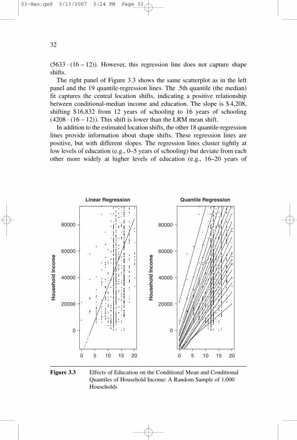
Using a random sample of 1,000 households from the total sample andthe fitted line based on the LRM, the left panel of Figure 3.3 presentsthe scatterplot of household income against the head of household’s yearsof schooling. The single regression line indicates mean shifts, for example,a mean shift of $ 22,532 from 12 years of schooling to 16 years of schooling

03-Hao.qxd 3/13/2007 5:24 PM Page 30

31

TAB

LE

3.2

Qua

ntile

-Reg

ress

ion

Est

imat

es f

or H

ouse

hold

Inc

ome

on E

duca

tion

(1)

(2)

(3)

(4)

(5)

(6)

(7)

(8)

(9)

(10)

(11)

(12)

(13)

(14)

(15)

(16)

(17)

(18)

(19)

ED

1,01

91,

617

2,02

32,

434

2,75

03,

107

3,39

73,

657

3,94

84,

208

4,41

84,

676

4,90

55,

214

5,55

75,

870

6,37

36,

885

8,38

5(2

8)(3

1)(4

0)(3

9)(4

4)(5

1)(5

7)(6

4)(6

6)(7

2)(8

1)(9

2)(8

8)(1

02)

(127

)(1

38)

(195

)(2

74)

(463

)

Con

stan

t−

4,25

2−7

,648

−9,1

70−1

1,16

0−1

2,05

6−1

3,30

8−1

3,78

3−1

3,72

6−1

4,02

6−1

3,76

9−1

2,54

6−1

1,55

7−9

,914

−8,7

60−7

,371

−4,2

27−1

,748

4,75

510

,648

(380

)(4

24)

(547

)(5

27)

(593

)(6

93)

(764

)(8

66)

(884

)(9

69)

(1,0

84)

(1,2

26)

(1,1

69)

(1,3

58)

(1,6

90)

(1,8

28)

(2,5

82)

(3,6

19)

(6,1

01)

NO

TE

:Sta

ndar

d er

rors

in p

aren

thes

es.

TAB

LE

3.3

Qua

ntile

-Reg

ress

ion

Est

imat

es f

or H

ouse

hold

Inc

ome

on R

ace

(1)

(2)

(3)

(4)

(5)

(6)

(7)

(8)

(9)

(10)

(11)

(12)

(13)

(14)

(15)

(16)

(17)

(18)

(19)

BL

AC

K−3

,124

−5,6

49−7

,376

−8,8

48−9

,767

−11,

232

−12,

344

−13,

349

−14,

655

−15,

233

−16,

459

−17,

417

−19,

053

−20,

314

−21,

879

−22,

914

−26,

063

−29,

951

−40,

639

(304

)(3

06)

(421

)(4

85)

(584

)(5

36)

(609

)(7

08)

(781

)(7

65)

(847

)(8

87)

(1,0

50)

(1,0

38)

(1,1

91)

(1,2

21)

(1,4

35)

(1,9

93)

(3,5

73)

Con

stan

t8,

556

12,4

8616

,088

19,7

1823

,198

26,8

3230

,354

34,0

2438

,047

41,9

9746

,635

51,5

1556

,613

62,7

3869

,680

77,8

7087

,996

102,

981

132,

400

(115

)(1

16)

(159

)(1

83)

(220

)(2

02)

(230

)(2

68)

(295

)(2

89)

(320

)(3

35)

(397

)(3

92)

(450

)(4

61)

(542

)(7

53)

(1,3

50)

NO

TE

:Sta

ndar

d er

rors

in p

aren

thes

es.

03-Hao.qxd 3/13/2007 5:24 PM Page 31

32

Quantile Regression

80000

60000

40000

20000

0

Ho

use

ho

ld In

com

e

Linear Regression

0 5 10 15 20

80000

60000

40000

20000

0

Ho

use

ho

ld In

com

e

0 5 10 15 20

Figure 3.3 Effects of Education on the Conditional Mean and ConditionalQuantiles of Household Income: A Random Sample of 1,000Households

(5633 · (16 – 12)). However, this regression line does not capture shapeshifts.

The right panel of Figure 3.3 shows the same scatterplot as in the leftpanel and the 19 quantile-regression lines. The .5th quantile (the median)fit captures the central location shifts, indicating a positive relationshipbetween conditional-median income and education. The slope is $ 4,208,shifting $16,832 from 12 years of schooling to 16 years of schooling(4208 · (16 – 12)). This shift is lower than the LRM mean shift.

In addition to the estimated location shifts, the other 18 quantile-regressionlines provide information about shape shifts. These regression lines arepositive, but with different slopes. The regression lines cluster tightly atlow levels of education (e.g., 0–5 years of schooling) but deviate from eachother more widely at higher levels of education (e.g., 16–20 years of

03-Hao.qxd 3/13/2007 5:24 PM Page 32

schooling). A shape shift is described by the tight cluster of the slopes atlower levels of education and the scattering of slopes at higher levels ofeducation. For instance, the spread of the conditional income on 16 yearsof schooling (from $12,052 for the .05th conditional quantile to $144,808for the .95th conditional quantile) is much wider than that on 12 years ofschooling (from $7,976 for the .05th conditional quantile to $111,268 forthe .95th conditional quantile). Thus, the off-median conditional quantilesisolate the location shift from the shape shift. This feature is crucial fordetermining the impact of a covariate on the location and shape shifts of theconditional distribution of the response, a topic discussed in Chapter 5 withthe interpretation of the QRM results.

QR Estimation

We review least-squares estimation so as to place QR estimation in a famil-iar context. The least-squares estimator solves for the parameter estimatesβ 0 and β 1 by taking those values of the parameters that minimize the sumof squared residuals:

min ∑i(yi – ( β0+β 1 xi ) )2. [3.3]

If the LRM assumptions are correct, the fitted response functionβ 0 + β 1 approaches the population conditional mean E( y⏐x) as the samplesize goes to infinity. In Equation 3.3, the expression minimized is the sumof squared vertical distances between data points ( x i , y i ) and the fitted liney = β 0 + β 1x.

A closed-form solution to the minimization problem is obtained by(a) taking partial derivatives of Equation 3.3 with respect to β0 and β1,respectively; (b) setting each partial derivative equal to zero; and (c) solv-ing the resulting system of two equations with two unknowns. We thenarrive at the two estimators:

A significant departure of the QR estimator from the LR estimator is thatin the QR, the distance of points from a line is measured using a weightedsum of vertical distances (without squaring), where the weight is 1 – p forpoints below the fitted line and p for points above the line. Each choice

β1 =

n∑i

(xi − x)(yi − y---)

n∑i

(xi − x)2

, β0 = y--- − β1x.

33

03-Hao.qxd 3/13/2007 5:24 PM Page 33

for this proportion p, for example, p = .10, .25, .50, gives rise to a differentfitted conditional-quantile function. The task is to find an estimator with thedesired property for each possible p. The reader is reminded of the discus-sion in Chapter 2 where it was indicated that the mean of a distribution canbe viewed as the point that minimizes the average squared distance over thepopulation, whereas a quantile q can be viewed as the point that minimizesan average weighted distance, with weights depending on whether the pointis above or below the value q.

For concreteness, we first consider the estimator for the median-regressionmodel. In Chapter 2, we described how the median (m) of y can be viewed as the minimizing value of E|y – m|. For an analogous prescription in themedian-regression case, we choose to minimize the sum of absolute residu-als. In other words, we find the coefficients that minimize the sum of absoluteresiduals (the absolute distance from an observed value to its fitted value).The estimator solves for the βs by minimizing Equation 3.4:

∑i ⎢yi – β0 – β1xi ⎢. [3.4]

Under appropriate model assumptions, as the sample size goes to infin-ity, we obtain the conditional median of y given x at the population level.

When expression Equation 3.4 is minimized, the resulting solution,which we refer to as the median-regression line, must pass through a pairof data points with half of the remaining data lying above the regressionline and the other half falling below. That is, roughly half of the residualsare positive and half are negative. There are typically multiple lines withthis property, and among these lines, the one that minimizes Equation 3.4is the solution.

Algorithmic Details

In this subsection, we describe how the structure of the function Equation3.4 makes it amenable to finding an algorithm for its minimization. Readerswho are not interested in this topic can skip this section.

The left panel of Figure 3.4 shows eight hypothetical pairs of data points(xi, yi) and the 28 lines (8(8 − 1)/2 = 28) connecting a pair of these pointsis plotted. The dashed line is the fitted median-regression line, that is, theline that minimizes the sum of absolute vertical distance from all datapoints. Observe that of the six points not falling on the median-regressionline, half of the points are below it and the other half are above it. Everyline in the (x, y) plane takes the form y = β0 + β1x for some choice ofintercept-slope pair ( β0 , β 1), so that we have a correspondence betweenlines in the (x, y) plane and points in the ( β0 , β 1) plane. The right panel

34

03-Hao.qxd 3/13/2007 5:24 PM Page 34

of Figure 3.4 shows a plot in the ( β0, β 1) plane that contains a pointcorresponding to every line in the left panel. In particular, the solid circleshown in the right panel corresponds to the median-regression line in theleft panel.

In addition, if a line with intercept and slope ( β0, β1) passes through agiven point (x i , yi), then yi = β0 + β1x i, so that (β0, β1) lies on the line β1 =( yi /xi) – (1/xi)β0. Thus, we have established a correspondence betweenpoints in the (x, y) plane and lines in the ( β0, β1) plane and vice versa, aphenomenon referred to as point/line duality (Edgeworth, 1888).

The eight lines shown in the right panel of Figure 3.4 correspond to theeight data points in the left panel. These lines divide the ( β0, β 1) plane intopolygonal regions. An example of such a region is shaded in Figure 3.4. Inany one of these regions, the points correspond to a family of lines in the (x, y) plane, all of which divide the data set into two sets in exactly thesame way (meaning that the data points above one line are the sameas the points above the other). Consequently, the function of (β0, β1) that weseek to minimize in Equation 3.4 is linear in each region, so that this func-tion is convex with a graph that forms a polyhedral surface, which is plot-ted from two different angles in Figure 3.5 for our example. The vertices,

35

4

2

−2

−2 −1 0 1 2 −8 −4 0 4 8

0

X

0

−4

4

8

−8

β1

β0

Y

Figure 3.4 An Illustration of Point/Line Duality

03-Hao.qxd 3/13/2007 5:24 PM Page 35

edges, and facets of the surface project to points, line segments, and regions,respectively, in the (β0, β1) plane shown in the right-hand panel of Figure 3.4.Using the point/line duality correspondence, each vertex corresponds to a lineconnecting a pair of data points. An edge connecting two vertices in the sur-face corresponds to a pair of such lines, where one of the data points definingthe first line is replaced by another data point, and the remaining points main-tain their position (above or below) relative to both lines.

An algorithm for minimization of the sum of absolute distances inEquation 3.4, one thus leading to the median-regression coefficients (β 0, β 1 ) ,can be based on exterior-point algorithms for solving linear-programmingproblems. Starting at any one of the points (β0, β1) corresponding to a vertex, the minimization is achieved by iteratively moving from vertex to

36

Figure 3.5 Polyhedral Surface and Its Projection

ββ1

ββ1

ββ0

ββ0

03-Hao.qxd 3/13/2007 5:24 PM Page 36

vertex along the edges of the polyhedral surface, choosing at each vertexthe path of the steepest descent until arriving at the minimum. Using thecorrespondence described in the previous paragraph, we iteratively movefrom line to line defined by pairs of data points, at each step deciding whichnew data point to swap with one of the two current ones by picking the onethat leads to the smallest value in Equation 3.4. The minimum sum ofabsolute errors is attained at the point in the ( β0, β1 ) plane below the lowestvertex of the surface. A simple argument involving the directional derivativewith respect to β0 (similar to the one in Chapter 2 showing that the median isthe solution to a minimization problem) leads to the conclusion that the samenumber of data points lie above the median-regression line as lie below it.

The median-regression estimator can be generalized to allow for pthquantile-regression estimators (Koenker & d’Orey, 1987). Recall from thediscussion in Chapter 2 that the pth quantile of a univariate sample y1, . . . , yn

distribution is the value q that minimizes the sum of weighted distances fromthe sample points, where points below q receive a weight of 1 – p and pointsabove q receive a weight of p. In a similar manner, we define the pth quantile-regression estimators β 0

(p) and β 1(p) as the values that minimize the weighted

sum of distances between fitted values yi = β 0(p) + β 1

(p)xi and the yi, where weuse a weight of 1 – p if the fitted value underpredicts the observed value yi

and a weight of p otherwise. In other words, we seek to minimize a weightedsum of residuals yi – yi where positive residuals receive a weight of p andnegative residuals receive a weight of 1 – p. Formally, the pth quantile-regression estimators β 0

(p) and β 1(p) are chosen to minimize

[3.5]

where dp is the distance introduced in Chapter 2. Thus, unlike Equation 3.4,which states that the negative residuals are given the same importance asthe positive residuals, Equation 3.5 assigns different weights to positive andnegative residuals. Observe that in Equation 3.5, the first sum is the sum ofvertical distances of data points from the line y = β 0

(p) + β 1(p) x, for points

lying above the line. The second is a similar sum over all data points lyingbelow the line.

Observe that, contrary to a common misconception, the estimation ofcoefficients for each quantile regression is based on the weighted dataof the whole sample, not just the portion of the sample at that quantile.

n∑i=1

dp(yi, yi) = p∑

yi≥β(p)0 +β

(p)1 xi

|yi − β(p)

0 − β(p)

1 xi | + (1 − p)

∑yi<β

(p)0 +β

(p)1 xi

|yi − β(p)

0 − β(p)

1 xi |,

37

03-Hao.qxd 3/13/2007 5:24 PM Page 37

An algorithm for computing the quantile-regression coefficients β 0( p) and

β 1(p) can be developed along lines similar to those outlined for the median-

regression coefficients. The pth quantile-regression estimator has a similarproperty to one stated for the median-regression estimator: The proportionof data points lying below the fitted line y = β 0

(p)+β 1(p)x is p, and the pro-

portion lying above is 1 – p.For example, when we estimate the coefficients for the .10th quantile-

regression line, the observations below the line are given a weight of .90and the ones above the line receive a smaller weight of .10. As a result, 90%of the data points (xi,yi) lie above the fitted line leading to positive residuals,and 10% lie below the line and thus have negative residuals. Conversely, toestimate the coefficients for the .90th quantile regression, points below theline are given a weight of .10, and the rest have a weight of .90; as a result,90% of observations have negative residuals and the remaining 10% havepositive residuals.

Transformation and Equivariance

In analyzing a response variable, researchers often transform the scale toaid interpretation or to attain a better model fit. Equivariance properties ofmodels and estimates refer to situations when, if the data are transformed,the models or estimates undergo the same transformation. Knowledge ofequivariance properties helps us to reinterpret fitted models when we trans-form the response variable.

For any linear transformation of the response variable, that is, the additionof a constant to y or the multiplication of y by a constant, the conditionalmean of the LRM can be exactly transformed. The basis for this statementis the fact that for any choice of constants a and c, we can write

E(c + ay |x) = c + aE(y |x). [3.6]

For example, if every household in the population received $500 fromthe government, the conditional mean would also be increased by $500 (thenew intercept would be increased by $500). When the $1 unit of income istransformed to the $1,000 unit, the conditional mean in the $1 unit isincreased by 1,000 times as well (the intercept and the slope are both mul-tiplied by 1,000 to be on the dollar scale). Similarly, if the dollar unit forwage rate is transformed to the cent unit, the conditional mean (the inter-cept and the slope) is divided by 100 to be on the dollar scale again. Thisproperty is termed linear equivariance because the linear transformation is

38

03-Hao.qxd 3/13/2007 5:24 PM Page 38

the same for the dependent variable and the conditional mean. The QRMalso has this property:

Q(p)(c + ay |x) = c + a (Q(p)[y | x]), [3.7]

provided that a is a positive constant. If a is negative, we haveQ(p) (c + ay | x) = c + a(Q (1− p)[ y|x]) because the order is reversed.

Situations often arise in which nonlinear transformation is desired.Log transformations are frequently used to address the right-skewness ofa distribution. Other transformations are considered in order to make adistribution appear more normal or to achieve a better model fit.

Log transformations are also introduced in order to model a covariate’seffect in relative terms (e.g., percentage changes). In other words, the effect ofa covariate is viewed on a multiplicative scale rather than on an additive one.In our example, the effects of education or race were previously expressed inadditive terms (the dollar unit), and it may be desirable to measure an effect inmultiplicative terms, for example, in terms of percentage changes. For exam-ple, we can ask: What is the percentage change in conditional-mean incomebrought about by one more year of schooling? The coefficient for education ina log income equation (multiplied by 100) approximates the percentagechange in conditional-mean income brought about by one more year ofschooling. However, under the LRM, the conditional mean of log income isnot the same as the log of conditional-mean income. Estimating two LRMsusing income and log income yields two fitted models:

y = –23,127 + 5,633ED, log y = 8.982 + .115ED.

The result from the log income model suggests that one more year ofeducation increases the conditional-mean income by about 11.5%.4 Theconditional mean of the income model at 10 years of schooling is $33,203,the log of which becomes 8.108. The conditional mean of the log incomemodel at the same schooling level is 10.062, a much larger figure than thelog of the conditional mean of income (8.108). While the log transforma-tion of a response in the LRM allows an interpretation of LRM estimates asa percentage change, the conditional mean of the response in absolute termsis impossible to obtain from the conditional mean on the log scale:

E(log y ⎢x) ≠ log [E( y ⎢x )] and E(yi ⎢xi) ≠ eE[log yi ⎢xi ]. [3.8]

Specifically, if our aim is to estimate the education effect in absoluteterms, we use the income model, whereas for the impact of education in

39

03-Hao.qxd 3/13/2007 5:24 PM Page 39

relative terms, we use the log income model. Although the two objectivesare related to each other, the conditional means of the two models are notrelated through any simple transformation.5 Thus, it would be a mistake touse the log income results to make conclusions about the distribution ofincome (though this is a widely used practice).

The log transformation is one member of the family of monotone trans-formations, that is, transformations that preserve order. Formally, a trans-formation h is a monotone if h (y) < h(y′) whenever y < y′. For variablestaking positive values, the power transformation h (y) = yφ is monotone fora fixed positive value of the constant φ. As a result of nonlinearity, when weapply a monotone transformation, the degree to which the transformationchanges the value of y can differ from one value of y to the next. While theproperty in Equation 3.6 holds for linear functions, it is not the case forgeneral monotone functions, that is, E(h (y)|x) ≠ h (E(yi|xi)). Generallyspeaking, the “monotone equivariance” property fails to hold for condi-tional means, so that LRMs do not possess monotone equivariance.

By contrast, the conditional quantiles do possess monotone equivariance;that is, for a monotone function h, we have

Q(p)(h (y) ⎢x) = h (Q(p)[y|x]). [3.9]

This property follows immediately from the version of monotone equi-variance stated for univariate quantiles in Chapter 2. In particular, a condi-tional quantile of log y is the log of the conditional quantile of y:

Q(p)(log(y) ⎢x) = log (Q(p)[y|x]), [3.10]

and equivalently,

Q(p)(y ⎢x) = eQ(p)[log(y) ⎢x], [3.11]

so that we are able to reinterpret fitted quantile-regression modelsfor untransformed variables to quantile-regression models for trans-formed variables. In other words, assuming a perfect fit for the pth quantilefunction of the form Q(p)(y|x) = β0 + β1x, we have Q(p)(log y|x) =log(β0 + β1x), so that we can use the impact of a covariate expressed inabsolute terms to describe the impact of a covariate in relative terms andvice versa.

Take the conditional median as an example:

Q(.50)( yi ⎢EDi) = –13769 + 4208EDi, Q(.50) (log(yi) ⎢EDi ) = 8.966 + .123EDi .

40

03-Hao.qxd 3/13/2007 5:24 PM Page 40

The conditional median of income at 10 years of schooling is $28,311.The log of this conditional median, 10.251, is similar to the conditionalmedian of the log income equation at the same education level, 10.196.Correspondingly, when moving from log to raw scale, in absolute terms, theconditional median at 10 years of schooling from the log income equationis e10.916 = 28,481.

The QRM’s monotone equivariance is particularly important for researchinvolving skewed distributions. While the original distribution is distortedby the reverse transformation of log-scale estimates if the LRM is used, theoriginal distribution is preserved if the QRM is used. A covariate’s effecton the response variable in terms of percentage change is often used ininequality research. Hence, the monotone equivariance property allowsresearchers to achieve both goals: measuring percentage change caused bya unit change in the covariate and measuring the impact of this change onthe location and shape of the raw-scale conditional distribution.

Robustness

Robustness refers to insensitivity to outliers and to the violation of modelassumptions concerning the data y. Outliers are defined as some values ofy that do not follow the relationship for the majority values. Under theLRM, estimates can be sensitive to outliers. Earlier in the first section ofthis chapter, we presented an example showing how outliers of income dis-tribution distort the mean and the conditional mean. The high sensitivity ofthe LRM to outliers has been widely recognized. However, the practice ofeliminating outliers does not satisfy the objective of much social-scienceresearch, particularly inequality research.

In contrast, the QRM estimates are not sensitive to outliers.6 This robust-ness arises because of the nature of the distance function in Equation 3.5that is minimized, and we can state a property of quantile-regression esti-mates that is similar to a statement made in Chapter 2 about univariatequantiles. If we modify the value of the response variable for a data pointlying above (or below) the fitted quantile-regression line, as long as thatdata point remains above (or below) the line, the fitted quantile-regressionline remains unchanged. Stated another way, if we modify values of theresponse variable without changing the sign of the residual, the fitted lineremains the same. In this way, as for univariate quantiles, the influence ofoutliers is quite limited.

In addition, since the covariance matrix of the estimates is calculatedunder the normality assumption, the LRM’s normality assumption is neces-sary for obtaining the inferential statistics of the LRM. Violation of thenormality assumption can cause inaccuracy in standard errors. The QRM is

41

03-Hao.qxd 3/13/2007 5:24 PM Page 41

robust to distributional assumptions because the estimator weighs the localbehavior of the distribution near the specific quantile more than the remotebehavior of the distribution. The QRM’s inferential statistics can be distri-bution free (a topic discussed in Chapter 4). This robustness is important instudying phenomena of highly skewed distributions such as income, wealth,educational, and health outcomes.

Summary

This chapter introduces the basics of the quantile-regression model incomparison with the linear-regression model, including the model setup,the estimation, and the properties of estimates. The QRM inherits many ofthe properties of sample quantiles introduced in Chapter 2. We explain howLRM is inadequate for revealing certain types of effects of covariates on thedistribution of a response variable. We also highlight some of the key featuresof QRM. We present many of the important differences between the QRMand the LRM, namely, (a) multiple-quantile-regression fits versus single-linear-regression fits to data; (b) quantile-regression estimation that minimizesa weighted sum of absolute values of residuals as opposed to minimizing thesum of squares in least-squares estimation; and (c) the monotone equivari-ance and robustness to distributional assumptions in conditional quantilesversus the lack of these properties in the conditional mean. With these basics,we are now ready to move on to the topic of QRM inference.

Notes

1. The data are drawn from the 2001 panel of the Survey of Income andProgram Participation (SIPP). Household income is the annual income in2001. The analytic sample for Chapters 3 through 5 includes 19,390 whitehouseholds and 3,243 black households.

2. Q (q)(y i ⎢x i) = Q (q)(β 0( p) + x i β 1

( p) + ε i( p)) = β 0

( p) + x i β 1( p) + Q (q)

(εi(p)) = Q(p) (yi ⎢xi) + cp,q.3. The number of distinct quantile solutions, however, is bounded by the

finite sample size.4. Precisely, the percentage change is 100(e.115–1) = 12.2%.5. The conditional mean is proportional to the exponential of the linear

predictor (Manning, 1998). For example, if the errors are normally distrib-uted N(0, σε

2), then E(yi ⎢xi) = eβ0 + β1xi+ 0.5σ ε

2

. The term e0.5σ ε2

is sometimescalled the smearing factor.

6. Note that this robustness does not apply to outliers of covariates.

42

03-Hao.qxd 3/13/2007 5:24 PM Page 42