3-phase Power Analysis Software Instruction Manual
92
Instruction Manual 3-phase Power Analysis Software
Transcript of 3-phase Power Analysis Software Instruction Manual
Instruction Manual 3-phase Power Analysis Software

3-phase Power Analysis Software Instruction Manual © 2021 Teledyne LeCroy, Inc. All rights reserved.
Unauthorized duplication of Teledyne LeCroy documentation materials is strictly prohibited. Users are permitted to duplicate and distribute Teledyne LeCroy documentation for internal educational purposes only.
X-Stream, ProBus, HDO and Teledyne LeCroy are trademarks of Teledyne LeCroy, Inc. Other product or brand names are trademarks or requested trademarks of their respective holders. Information in this publication supersedes all earlier versions. Specifications are subject to change without notice.
3-phase-power-sim-eng_01jun21.pdf June, 2021

Instruction Manual
i
Table of Contents Introduction ............................................................................................................................................................... 1
Supported Inputs ................................................................................................................................................................ 3 Choosing the Best Input Method for Your Signals ........................................................................................................... 3
Direct BNC Cable Connections .................................................................................................................................. 3 Passive Voltage Probes ............................................................................................................................................. 4 High-Voltage (HV) Passive Voltage Probes .............................................................................................................. 4 Active Single-Ended Voltage Probes ......................................................................................................................... 4 Active Differential Voltage Probes ............................................................................................................................ 4 High-Voltage Differential Probes ............................................................................................................................... 4 Current Probes ............................................................................................................................................................ 5 CA10 ProBus Current Adapter ................................................................................................................................... 5
Using the 3-phase Power Analysis Software ............................................................................................................. 6 Accessing the Software...................................................................................................................................................... 6 3-phase Power Analysis Dialog .......................................................................................................................................... 7 Input and Output Dialogs ................................................................................................................................................... 8
Wiring Configuration .................................................................................................................................................. 9 Voltage and Current Assignments ......................................................................................................................... 12 Harmonic Filter ........................................................................................................................................................ 12 Sync Signal .............................................................................................................................................................. 15
DC Bus Dialog .................................................................................................................................................................... 28 Numerics Dialog and Table .............................................................................................................................................. 29
Table Rows ............................................................................................................................................................... 29 Table Columns ......................................................................................................................................................... 30 Displayed Units ........................................................................................................................................................ 30 Creating Per-Cycle Waveforms from the Numerics Table .................................................................................... 31
Waveforms + Stats Dialog and Statistics Table ............................................................................................................. 32 Per-cycle Waveforms .............................................................................................................................................. 32 Statistics Table ........................................................................................................................................................ 33 Measure Parameter Definitions ............................................................................................................................. 34
Zoom+Gate Mode ............................................................................................................................................................. 35 Accessing Zoom+Gate ............................................................................................................................................ 35 Zoom+Gate Example ............................................................................................................................................... 35
Harmonics Calculation Option ................................................................................................................................. 37 Harmonics Calculation Overview ..................................................................................................................................... 37 Harmonic Filtering – Input and Output Dialogs ............................................................................................................. 38 Numerics Table THD Measurement Parameters ............................................................................................................ 40 Harmonics Calc Setup Dialog .......................................................................................................................................... 41
Harmonics Calc Setup and Fundamental Frequency Detection ......................................................................... 41 Harmonics Table Display ........................................................................................................................................ 42 Units/Limits ............................................................................................................................................................. 43 Spectrum Zoom ....................................................................................................................................................... 44

3-phase Power Analysis Software
ii
Harmonics Order Table..................................................................................................................................................... 44 Spectral Waveform Display .............................................................................................................................................. 46
Vector Display Option .............................................................................................................................................. 48 Harmonic Filtering ............................................................................................................................................................ 48 Line Neutral Conversion ................................................................................................................................................... 48 Vector Calculation Method .............................................................................................................................................. 50
Arithmetic Average ................................................................................................................................................... 50 Vector Average ......................................................................................................................................................... 50
Waveform Transformations Option .......................................................................................................................... 51 Transformation Types ...................................................................................................................................................... 51 Applying Transformations................................................................................................................................................ 51
Appendix A: Measurement Best Practices ............................................................................................................... 53 Allow for Recommended Warm-up Times ...................................................................................................................... 53 Auto Zero Differential Probes .......................................................................................................................................... 54 Degauss Current Probes .................................................................................................................................................. 54 Deskew non-Teledyne LeCroy Current or Voltage Measurement Devices ................................................................... 55 Choose the Best Sync Signal for Measurements ........................................................................................................... 55 Avoid Non-Zero Offset Values.......................................................................................................................................... 56 Maximize Use of Vertical Grid .......................................................................................................................................... 56 Compensate Passive Probes ........................................................................................................................................... 56 Apply Filters to Lower Noise ............................................................................................................................................ 57 Deskew Teledyne LeCroy Probes .................................................................................................................................... 57
Appendix B: Calculation Methods and Formulas ...................................................................................................... 58 Impact of Wiring Configuration on Calculations ............................................................................................................ 58
Three Wattmeter Measurements ............................................................................................................................ 58 Two Wattmeter Measurements............................................................................................................................... 58 One Wattmeter Measurements ............................................................................................................................... 58
Impact of Zoom+Gate on Calculations ........................................................................................................................... 59 Impact of Harmonic Filtering on Calculations................................................................................................................ 59 Notational Conventions .................................................................................................................................................... 59 3-phase 4-wire (3V3A) Calculations ................................................................................................................................ 61 3-phase 3-wire (3V3A) Calculations ................................................................................................................................ 65 3-phase 3-wire (2V2A) Calculations ................................................................................................................................ 69 1-phase 3-wire (2V2A) Calculations ................................................................................................................................ 73 1-phase 2-wire Wiring Configuration Calculations ......................................................................................................... 76 Harmonics Calculation Option Formulas ........................................................................................................................ 78
Conventions .............................................................................................................................................................. 78 Harmonics Order Table Format ............................................................................................................................... 79 Harmonics Order Table Calculations ...................................................................................................................... 80 THD Measurement Calculations (Numerics Table) ............................................................................................... 82

Instruction Manual
1
Introduction Teledyne LeCroy’s 3-phase Power Analysis is a software package that provides complete 3-phase electrical power analysis. Calculations can be performed on any building block (AC-AC, AC-DC, DC-DC, DC-AC) of a Power Conversion system. Static power results can be displayed in a Numeric table, Statistics table, while dynamic power can be displayed as synthesized per-cycle Waveforms that are time correlated to the originally acquired data. Zoom+Gate functionality is included to permit calculations on a smaller portion of a larger acquisition record. As the zoom window is changed, the Numerics table results are updated instantly without the need to reacquire the waveforms. Key features include:
• Complete 3-phase system debug and validation for solar PV inverters, grid-tied inverters, uninterruptible power supplies (UPS), welding equipment, power conversion systems, DC-DC power supplies, etc.
• Measurements for real, apparent and reactive power and efficiency
• Support for two-wattmeter and three-wattmeter methods
• Optional Harmonics calculations and filtering
• Compatible with 4-channel as well as 8-channel high definition oscilloscope models
Signals are input to any of the oscilloscope’s analog channels through a simple BNC/cable connection with 50 Ω or 1 MΩ coupling, passive probe connection with 1 MΩ coupling, or Teledyne LeCroy-compatible voltage or current probe. Digital signals may also be input on instruments with Mixed Signal capabilities. Adapters are available to conveniently rescale current signals from other devices (e.g., current transformers, current transducers, Rogoswki coils, etc.) to Ampere units and values when connected to the analog channels.
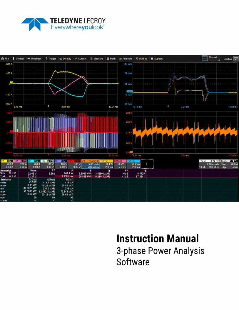
As voltage and current signals are acquired, the 3-phase Power Analysis software automatically performs cyclical analysis of the acquired signals using a user-specified “Sync” signal. This determines the measurement interval at which voltage, current and power values will be computed. Figure 1 is an example of a 3-phase set of line-line voltage and line current signals with the blue, sinusoidal current trace selected as the “Sync” signal.
Once measurement intervals are defined and applied across all waveforms in an acquisition, mathematical calculations are then performed for each measurement interval, with mean or average values calculated over N cycles for cycles i = 1 to N in the full or gated acquisition.
Mathematical operations are valid for both sinusoidal voltage and current waveforms, and non-sinusoidal (e.g., PWM or non-linear) waveforms. Voltage and current values are calculated per IEEE definitions. See Appendix B (p.58) for more detailed descriptions of the measurement calculations.
The mean or peak value (depending on the measurement) for a single acquisition is displayed in a user-defined Numerics table. Zoom+Gate functionality is included to permit calculations on a smaller portion of a larger
Figure 1: Sinusoidal “Sync” signal determines measurement interval for 3-phase set of signals.
3-phase Power Analysis Software
2
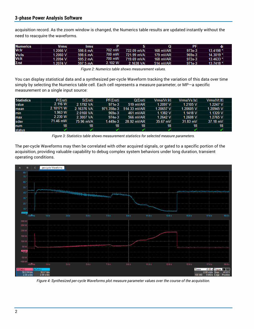
acquisition record. As the zoom window is changed, the Numerics table results are updated instantly without the need to reacquire the waveforms.
Figure 2: Numerics table shows measurement values.
You can display statistical data and a synthesized per-cycle Waveform tracking the variation of this data over time simply by selecting the Numerics table cell. Each cell represents a measure parameter, or MP—a specific measurement on a single input source:
Figure 3: Statistics table shows measurement statistics for selected measure parameters.
The per-cycle Waveforms may then be correlated with other acquired signals, or gated to a specific portion of the acquisition, providing valuable capability to debug complex system behaviors under long duration, transient operating conditions.
Figure 4: Synthesized per-cycle Waveforms plot measure parameter values over the course of the acquisition.
Instruction Manual
3
Supported Inputs The software may be used with Teledyne LeCroy instruments equipped with ProBusTM or ProBus2TM interfaces. The ProBus interface consists of a BNC and a 6-pin connector that will automatically:
• Identify and set attenuation for Teledyne LeCroy passive probes
• Power and identifiy ProBus-compatible probes, making correct selection of probe input coupling, attenuation, etc.
A variety of ProBus-compatible voltage and current measurement probes are supported for use with the 3-phase Power Analysis software. Differential voltage probes are available with high voltage isolation, excellent noise and flatness performance, and high common-mode rejection ratio (CMRR). Current probes are available with ratings up to 700 A (RMS, peak).
A wide variety of third-party voltage and current transformers/transducers may be integrated into the 3-phase Power Analysis software by using a direct BNC connection to the instrument and a rescale operation. A Current Adapter may be purchased from Teledyne LeCroy and programmed so that third-party current measurement devices are automatically re-scaled whenever connected to the instrument.
See Choosing the Best Input Method for Your Signals (below) for guidance on selecting the best input device.
Choosing the Best Input Method for Your Signals Direct BNC Cable Connections BNC cables are commonly used to connect current transducers/transformers (CT), Rogowski coils, voltage (potential) transformers (PT), or other sensor units to the input channels. A CT should have a resistor installed across the output so as to create a voltage which can be input to the instrument.
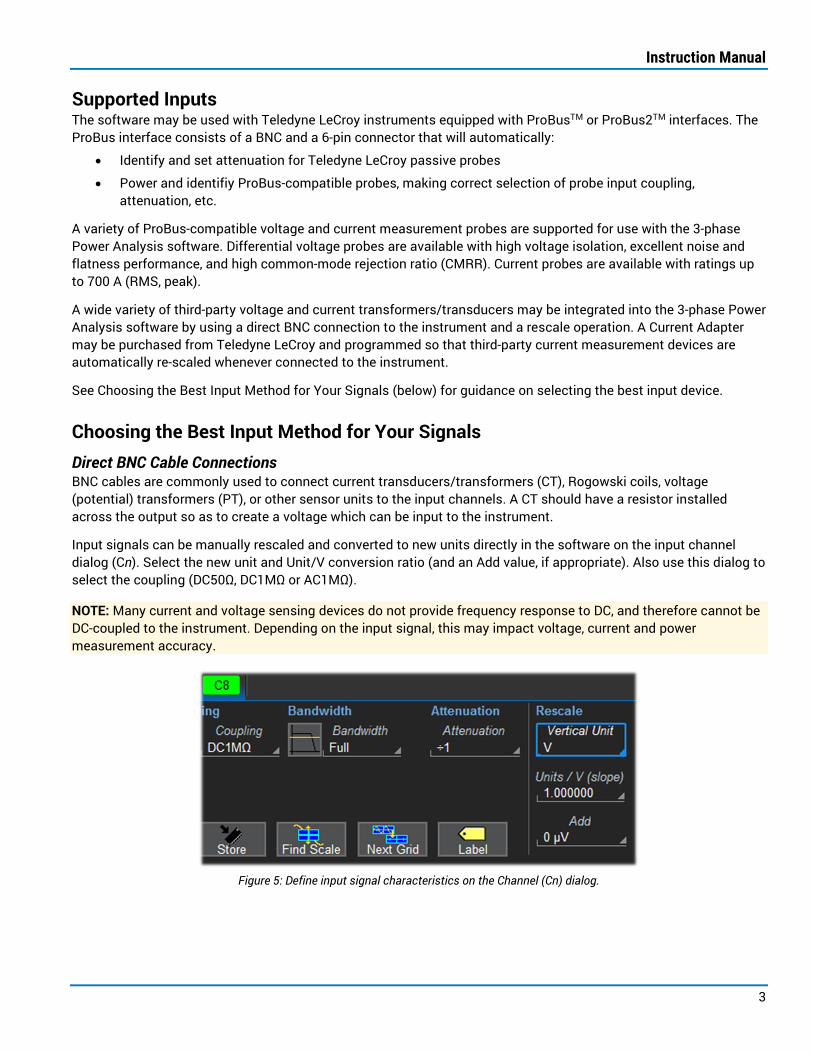
Input signals can be manually rescaled and converted to new units directly in the software on the input channel dialog (Cn). Select the new unit and Unit/V conversion ratio (and an Add value, if appropriate). Also use this dialog to select the coupling (DC50Ω, DC1MΩ or AC1MΩ).
NOTE: Many current and voltage sensing devices do not provide frequency response to DC, and therefore cannot be DC-coupled to the instrument. Depending on the input signal, this may impact voltage, current and power measurement accuracy.
Figure 5: Define input signal characteristics on the Channel (Cn) dialog.

3-phase Power Analysis Software
4
Passive Voltage Probes Passive probes utilize an attenuation-sense pin that identifies to the input channel the appropriate attenuation (and coupling) settings. Passive probes are single-ended, and the ground lead on a passive probe is connected directly to the instrument chassis ground. Therefore, the probe connection to the device under test (DUT) is also connected to instrument chassis ground.
High input resistance makes passive probes the ideal tool for low-frequency signals, since circuit loading at these frequencies is minimized. Passive probes are also ideal for measuring lower voltage signals referenced to ground. A common application for passive probes is measuring output voltages on a battery-powered device, where the output is effectively referenced to an earth ground. At higher voltages (>50 V), common-mode interference may introduce unwanted noise to the measurement. In these cases, a suitable differential voltage probe is usually recommended.
CAUTION: Do not use passive probes with the probe ground attached to a 3-phase system neutral connection, as the neutral voltage may not be the same as ground. Significant currents could travel from the passive probe neutral to instrument ground, creating a hazardous situation that could result in electric shock to the user or damage to the DUT. In this case, an HV-isolated, differential voltage probe is recommended.
High-Voltage (HV) Passive Voltage Probes These probes are similar to low-voltage passive probes, except they have a higher voltage rating at the probe tip and may require that you manually set the attenuation and coupling for the input channel. The same cautions about ground connections that apply to passive voltage probes apply to HV passive voltage probes. Two HV passive voltage probes may be used in a pseudo-differential mode by connecting the probe grounds to each other (not to ground) and the cables to two separate input channels. Create a math function subtracting one channel from the other to achieve the differential result, and use the function output as the voltage input source. While this technique may be the only suitable method for very high voltages, there can be significant common-mode interference.
Active Single-Ended Voltage Probes Compatible active probes utilize the Teledyne LeCroy ProBus interface to identify the probe to the input channel, so the correct attenuation and coupling are set automatically. However, these probes typically have much less voltage range and peak voltage capability than a passive probe. The same cautions about ground connections that apply to passive probes apply to active single-ended voltage probes, as well.
Active Differential Voltage Probes Differential voltage probes sense the voltage difference that appears between + and – inputs. The voltage component that is referenced to earth (the common mode voltage) is identical on both inputs and is rejected by the amplifier. These types of probes are ideal for measuring low voltages in control systems and gate-drive voltages, as long as the voltages are not “floating” more than the common-mode voltage rating of the probe. Where common-mode voltage is “floating” by a large amount, typically a high-voltage differential voltage probe is used.
High-Voltage Differential Probes High-voltage differential probes operate the same as “normal” differential voltage probes, but they have the added benefit of HV isolation with respect to ground and wider differential voltage ranges. They are also very cost effective, making them a good, general-purpose differential voltage probe for a variety of power electronics inverter subsystem and control system probing. Since these probes are rated for higher voltages, the tips are HV insulated and larger than normal differential voltage probes, so they might not be suitable for fine pitch probing. Also, bandwidths are usually lower (~100 MHz).
Instruction Manual
5
Current Probes Current probes use a combination of Hall effect and transformer technology, which enables measurements to be made on DC, AC and impulse currents at very high bandwidths. Teledyne LeCroy current probes are available with ratings up to 500 A continuous (700 A peak). They are designed to be used on insulated conductors, as the core and shield are grounded, and voltage applied to the probe may damage the probe or the circuit under test. Note that in the presence of strong magnetic fields, measurement accuracy may be affected, so it is good practice to locate these probes as far away from strong magnetic fields as is possible.
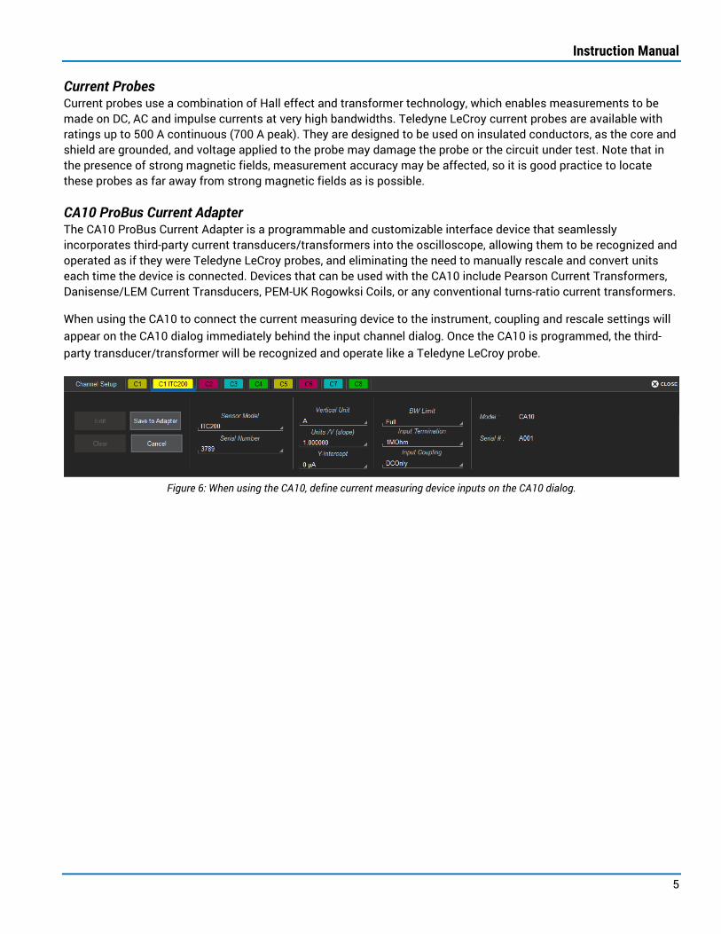
CA10 ProBus Current Adapter The CA10 ProBus Current Adapter is a programmable and customizable interface device that seamlessly incorporates third-party current transducers/transformers into the oscilloscope, allowing them to be recognized and operated as if they were Teledyne LeCroy probes, and eliminating the need to manually rescale and convert units each time the device is connected. Devices that can be used with the CA10 include Pearson Current Transformers, Danisense/LEM Current Transducers, PEM-UK Rogowksi Coils, or any conventional turns-ratio current transformers.
When using the CA10 to connect the current measuring device to the instrument, coupling and rescale settings will appear on the CA10 dialog immediately behind the input channel dialog. Once the CA10 is programmed, the third-party transducer/transformer will be recognized and operate like a Teledyne LeCroy probe.
Figure 6: When using the CA10, define current measuring device inputs on the CA10 dialog.
3-phase Power Analysis Software
6
Using the 3-phase Power Analysis Software Accessing the Software The 3-phase Power Analysis software package employs a multi-tabbed user interface. The tabs are referred to here as “setup dialogs”. These dialogs enable you to define the connection of signals for proper analysis, customize tables of measurements, and create per-cycle Waveforms tracking voltage, current and power measurements.
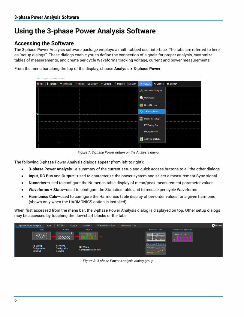
From the menu bar along the top of the display, choose Analysis > 3-phase Power.
Figure 7: 3-phase Power option on the Analysis menu.
The following 3-phase Power Analysis dialogs appear (from left to right):
• 3-phase Power Analysis—a summary of the current setup and quick access buttons to all the other dialogs
• Input, DC Bus and Output—used to characterize the power system and select a measurement Sync signal
• Numerics—used to configure the Numerics table display of mean/peak measurement parameter values
• Waveforms + Stats—used to configure the Statistics table and to rescale per-cycle Waveforms
• Harmonics Calc—used to configure the Harmonics table display of per-order values for a given harmonic (shown only when the HARMONICS option is installed)
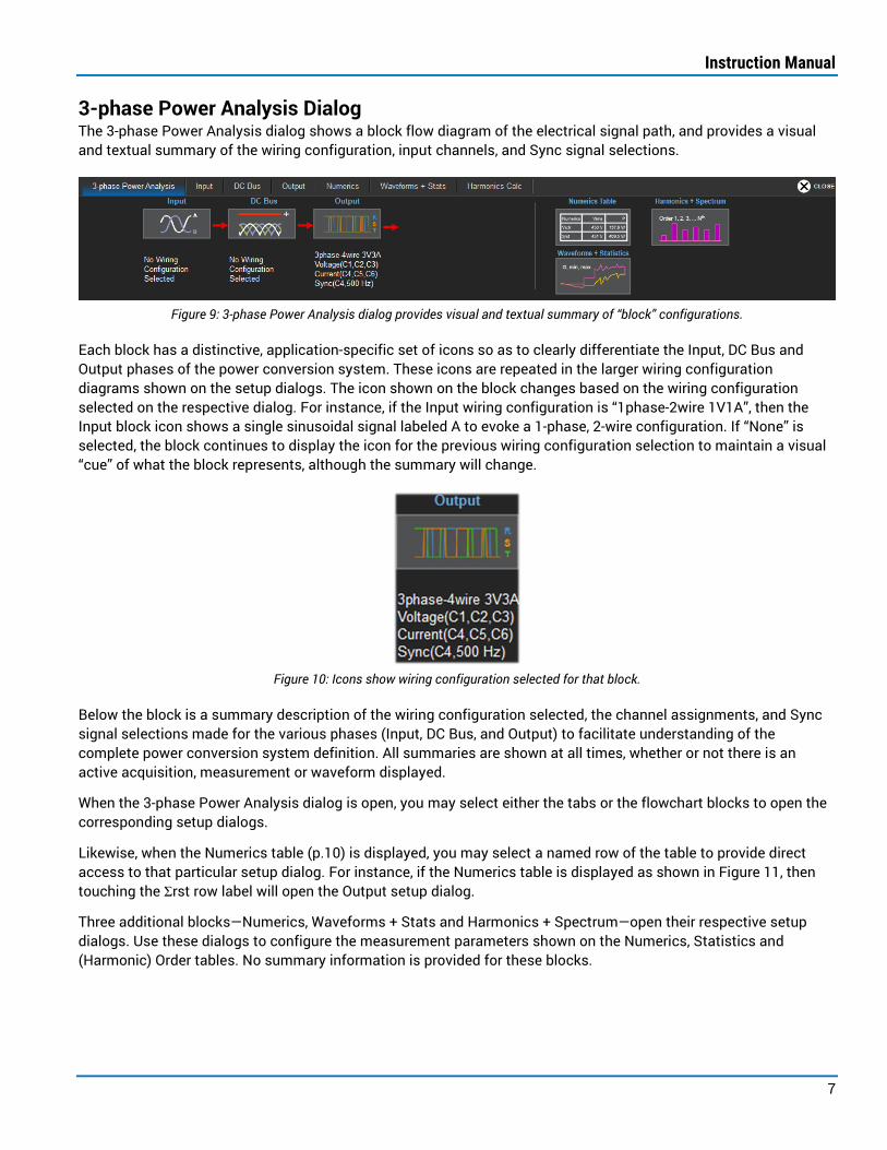
When first accessed from the menu bar, the 3-phase Power Analysis dialog is displayed on top. Other setup dialogs may be accessed by touching the flow-chart blocks or the tabs.
Figure 8: 3-phase Power Analysis dialog group.
Instruction Manual
7
3-phase Power Analysis Dialog The 3-phase Power Analysis dialog shows a block flow diagram of the electrical signal path, and provides a visual and textual summary of the wiring configuration, input channels, and Sync signal selections.
Figure 9: 3-phase Power Analysis dialog provides visual and textual summary of “block” configurations.
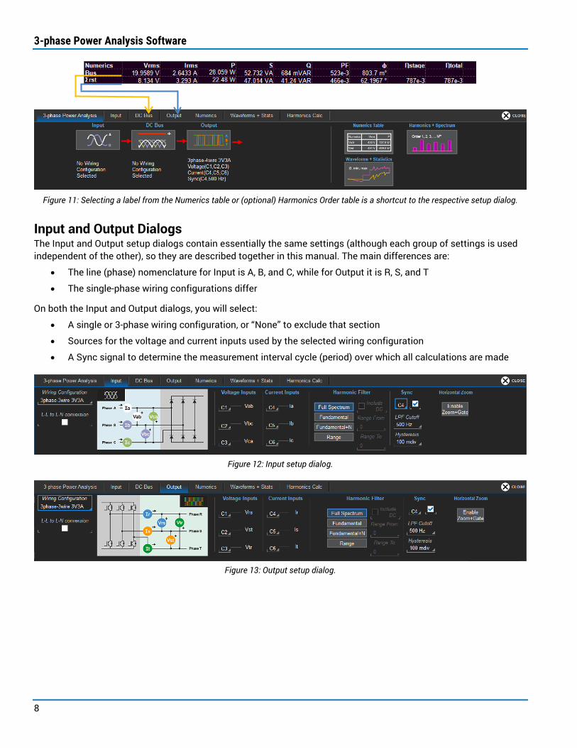
Each block has a distinctive, application-specific set of icons so as to clearly differentiate the Input, DC Bus and Output phases of the power conversion system. These icons are repeated in the larger wiring configuration diagrams shown on the setup dialogs. The icon shown on the block changes based on the wiring configuration selected on the respective dialog. For instance, if the Input wiring configuration is “1phase-2wire 1V1A”, then the Input block icon shows a single sinusoidal signal labeled A to evoke a 1-phase, 2-wire configuration. If “None” is selected, the block continues to display the icon for the previous wiring configuration selection to maintain a visual “cue” of what the block represents, although the summary will change.
Figure 10: Icons show wiring configuration selected for that block.
Below the block is a summary description of the wiring configuration selected, the channel assignments, and Sync signal selections made for the various phases (Input, DC Bus, and Output) to facilitate understanding of the complete power conversion system definition. All summaries are shown at all times, whether or not there is an active acquisition, measurement or waveform displayed.
When the 3-phase Power Analysis dialog is open, you may select either the tabs or the flowchart blocks to open the corresponding setup dialogs.
Likewise, when the Numerics table (p.10) is displayed, you may select a named row of the table to provide direct access to that particular setup dialog. For instance, if the Numerics table is displayed as shown in Figure 11, then touching the Σrst row label will open the Output setup dialog.
Three additional blocks—Numerics, Waveforms + Stats and Harmonics + Spectrum—open their respective setup dialogs. Use these dialogs to configure the measurement parameters shown on the Numerics, Statistics and (Harmonic) Order tables. No summary information is provided for these blocks.
3-phase Power Analysis Software
8
Figure 11: Selecting a label from the Numerics table or (optional) Harmonics Order table is a shortcut to the respective setup dialog.
Input and Output Dialogs The Input and Output setup dialogs contain essentially the same settings (although each group of settings is used independent of the other), so they are described together in this manual. The main differences are:
• The line (phase) nomenclature for Input is A, B, and C, while for Output it is R, S, and T
• The single-phase wiring configurations differ
On both the Input and Output dialogs, you will select:
• A single or 3-phase wiring configuration, or “None” to exclude that section
• Sources for the voltage and current inputs used by the selected wiring configuration
• A Sync signal to determine the measurement interval cycle (period) over which all calculations are made
Figure 12: Input setup dialog.
Figure 13: Output setup dialog.

Instruction Manual
9
Wiring Configuration To correctly calculate power values, identify the Wiring Configuration used by each power conversion system section, and assign input sources to each voltage and current.
Figure 14: Input 3-phase 3-wire 3V3A wiring configuration.
Input has these wiring configuration selections (plus “None”):
• 3-phase-4-wire 3V3A–use Line-Neutral or Line-Reference voltage probing
• 3-phase-3-wire 3V3A–use Line-Line voltage probing
• 3-phase-3-wire 2V2A–use Line-Line voltage probing and 2 wattmeter method
TIP: This method is ideal for measuring input/output efficiency, since if selected for both the Input and Output, it requires only eight total analog input channels (four voltage and four current).
• 1-phase-3-wire 2V2A
• 1-phase-2-wire 1V1A
Output has these wiring configuration selections (plus “None”):
• 3-phase-4-wire 3V3A–Use Line-Neutral or Line-Reference voltage probing.
• 3-phase-3-wire 3V3A–Use Line-Line voltage probing.
• 3-phase-3-wire (2 Voltage, 2 Current)–Use Line-Line voltage probing and 2 wattmeter method. This method is ideal for measuring input/output efficiency since, if selected for both the Input and Output, it requires only eight total (4 Voltage and 4 Current) analog input channels.
• 1-phase (Half Bridge)
• 1-phase (Full Bridge)
NOTE: Both two-wattmeter and three-wattmeter methods are supported on 8-channel oscilloscopes. Only two-wattmeter methods are supported on 4-channel oscilloscopes. 1-phase methods are supported on 4- and 8-channel oscilloscopes.
3-phase Power Analysis Software
10
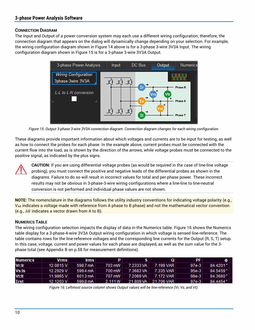
CONNECTION DIAGRAM The Input and Output of a power conversion system may each use a different wiring configuration, therefore, the connection diagram that appears on the dialog will dynamically change depending on your selection. For example, the wiring configuration diagram shown in Figure 14 above is for a 3-phase 3-wire 3V3A Input. The wiring configuration diagram shown in Figure 15 is for a 3-phase 3-wire 3V3A Output.
Figure 15: Output 3-phase 3-wire 3V3A connection diagram. Connection diagram changes for each wiring configuration.
These diagrams provide important information about which voltages and currents are to be input for testing, as well as how to connect the probes for each phase. In the example above, current probes must be connected with the current flow into the load, as is shown by the direction of the arrows, while voltage probes must be connected to the positive signal, as indicated by the plus signs.
CAUTION: If you are using differential voltage probes (as would be required in the case of line-line voltage probing), you must connect the positive and negative leads of the differential probes as shown in the diagrams. Failure to do so will result in incorrect values for total and per-phase power. These incorrect results may not be obvious in 3-phase-3-wire wiring configurations where a line-line to line-neutral conversion is not performed and individual phase values are not shown.
NOTE: The nomenclature in the diagrams follows the utility industry conventions for indicating voltage polarity (e.g., VAB indicates a voltage made with reference from A phase to B phase) and not the mathematical vector convention (e.g., 𝐴𝐴𝐴𝐴 indicates a vector drawn from A to B).
NUMERICS TABLE The wiring configuration selection impacts the display of data in the Numerics table. Figure 16 shows the Numerics table display for a 3-phase-4-wire 3V3A Output wiring configuration in which voltage is sensed line-reference. The table contains rows for the line-reference voltages and the corresponding line currents for the Output (R, S, T) setup. In this case, voltage, current and power values for each phase are displayed, as well as the sum value for the 3-phase total (see Appendix B on p.58 for measurement definitions).
Figure 16: Leftmost source column shows Output values will be line-reference (Vr, Vs, and Vt).

Instruction Manual
11
LINE-LINE TO LINE-NEUTRAL CONVERSION For wiring configurations that require voltage sensing line-line, the Numerics table will display line-line per-phase voltage and current values, but it will not display per-phase power values due to the voltage being sensed to a different reference (line-line) than the current (line).
However, it is possible to convert the voltage reference to a Line-Neutral basis, which then permits per-phase power calculations. Simply select the L-L to L-N conversion checkbox immediately below the Wiring Configuration (this checkbox is disabled when voltage is already sensed line-neutral or line-reference). Conversion has the benefit of allowing you to configure the Numerics table to display the per-phase power (P, S, Q, λ, and ϕ) values for each phase and converted line-neutral VRMS value (and other voltage values calculated on a line-neutral basis).
In Figure 17, the leftmost column of the table indicates voltage is line-line (Vrs, Vst, and Vtr) and currents are line currents (lr, ls, and lt):
Figure 17: Leftmost source column shows Output values will be line-line (Vrs, Vst, and Vtr).
When conversion is selected, the Numerics table data changes as shown in Figure 18.
Figure 18: Leftmost source column shows values have undergone L-L to L-N conversion.
Now, the voltage magnitude is in a Line-Neutral basis, and the phase has been corrected as well, which allows per-phase power values to be calculated. The leftmost column of the table indicates voltage as line voltage (Vr, Vs, and Vt) and there is an LL to LN notation next to each source indicating that these values were calculated using a mathematical conversion and not via direct measurement.
NOTE: The line-neutral conversion assumes a balanced 3-phase system in which the vectoral sum of all voltages is zero and the vectoral sum of all currents is zero. To perform the conversion, it enforces this assumption as a requirement, and the C (Input) or T (Output) current value will be adjusted to ensure that the vector sum of all currents is zero. Depending on the amount of adjustment to the C or T phase current reading, the total P (and S and Q) values will change slightly, as can be seen in Figure 18. If the Idc measurement parameter were displayed in the Numerics table, the adjustment could be quantified.
See Numerics Dialog (p.29) for more information on configuring the Numerics table.

3-phase Power Analysis Software
12
Voltage and Current Assignments An area for assigning sources to Voltage Inputs and Current Inputs appears on the Input, DC Bus, and Output dialogs. The voltages and currents listed depend on the wiring configuration chosen. Figure 19 shows the voltage and current assignments for a 3-phase 3-wire 2V2A Output wiring configuration.
Figure 19: Voltage and Current assignments.
In this case, each has only two assignments; the unnecessary third is disabled (“x”). C1 is the default source for all voltages and currents. Simply touch or click the source field and select the channel (Cn), memory (Mn), or math function (Fn) that is the correct source for that voltage or current.
CAUTION: Use care when changing from a 3-phase 3-wire 3V3A to a 3-phase 3-wire 2V2A wiring configuration. The input assignments look very similar, but the polarity of the CA or TR voltage is now reversed (by definition of the two wattmeter method) to AC or RT. This requires that you physically reconnect the differential voltage probe or Invert the input channel on the channel dialog, swap the selection of inputs to switch the signal polarity, and reassign a voltage. Failure to do this will result in an incorrect result.
Harmonic Filter The Input and Output setup dialogs contain selections for setting a Harmonic filter on the sources prior to measurement calculations.
Figure 20: Harmonic filter setup.
Two selections, Full Spectrum and Fundamental, are standard with the 3-phase Power Analysis software. The Fundamental+N and Range selections are enabled with the purchase of the THREEPHASEHARMONICS option.
Instruction Manual
13
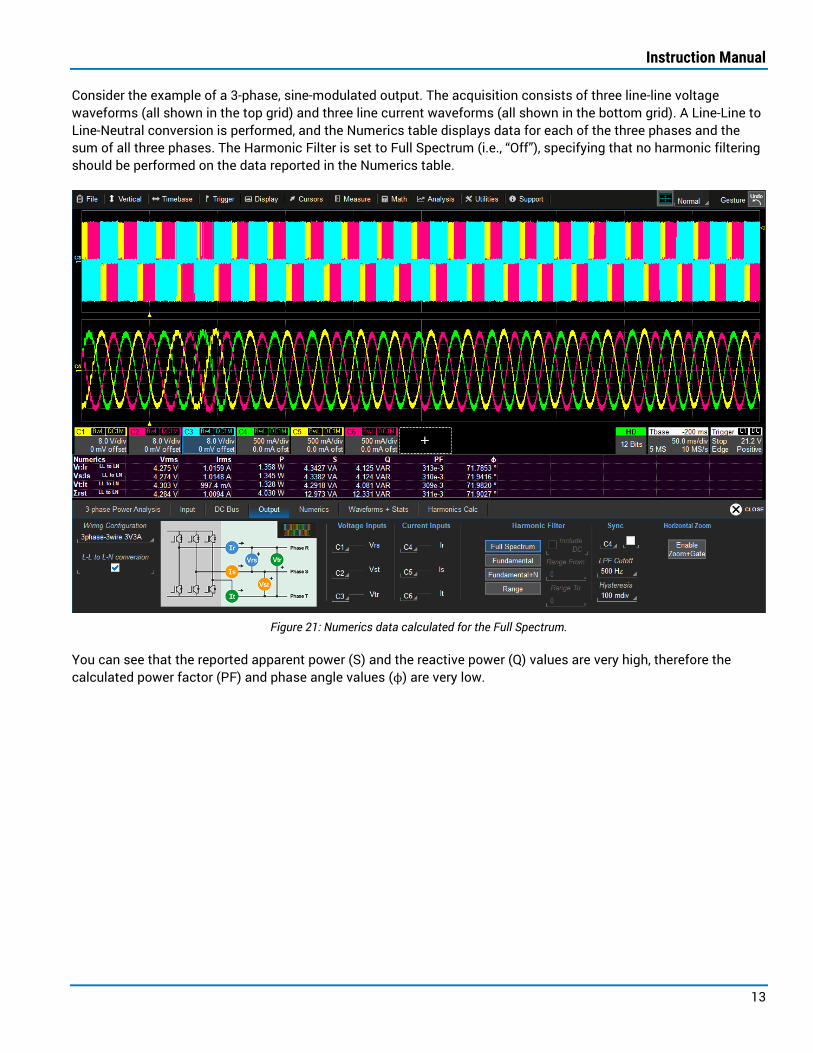
Consider the example of a 3-phase, sine-modulated output. The acquisition consists of three line-line voltage waveforms (all shown in the top grid) and three line current waveforms (all shown in the bottom grid). A Line-Line to Line-Neutral conversion is performed, and the Numerics table displays data for each of the three phases and the sum of all three phases. The Harmonic Filter is set to Full Spectrum (i.e., “Off”), specifying that no harmonic filtering should be performed on the data reported in the Numerics table.
Figure 21: Numerics data calculated for the Full Spectrum.
You can see that the reported apparent power (S) and the reactive power (Q) values are very high, therefore the calculated power factor (PF) and phase angle values (ϕ) are very low.
3-phase Power Analysis Software
14
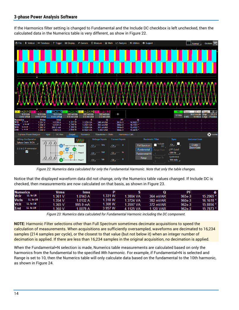
If the Harmonics filter setting is changed to Fundamental and the Include DC checkbox is left unchecked, then the calculated data in the Numerics table is very different, as show in Figure 22.
Figure 22: Numerics data calculated for only the Fundamental Harmonic. Note that only the table changes.
Notice that the displayed waveform data did not change, only the Numerics table values changed. If Include DC is checked, then measurements are now calculated on that basis, as shown in Figure 23.
Figure 23: Numerics data calculated for Fundamental Harmonic including the DC component.
NOTE: Harmonic Filter selections other than Full Spectrum sometimes decimate acquisitions to speed the calculation of measurements. When acquisitions are sufficiently oversampled, waveforms are decimated to 16,234 samples (214 samples per cycle), or the closest to that value (but not below it) when an integer number of decimation is applied. If there are less than 16,234 samples in the original acquisition, no decimation is applied.
When the Fundamental+N selection is made, Numerics table measurements are calculated based on only the harmonics from the fundamental to the specified Nth harmonic. For example, if Fundamental+N is selected and Range is set to 10, then the Numerics table will only calculate data based on the fundamental to the 10th harmonic, as shown in Figure 24.

Instruction Manual
15
Figure 24: Numerics data calculated for Fundamental to the 10th harmonic.
The Range setting is very similar to the Fundamental+N setting, except it allows a starting harmonic order to be specified. This provides a method to make measurements on a range of harmonic orders that don’t necessarily include the fundamental.
Sync Signal In order to perform power, voltage and current measurements over individual cycles, a measurement interval must first be determined. For each power conversion section, you will choose a Sync signal that determines the measurement interval (the default is the signal on C1). This Sync signal can be filtered to remove high-frequency content and obtain better periodicity.
Figure 25: Sync signal setup.
HOW THE SYNC SIGNAL IS USED The software determines a 50% amplitude value for the Sync signal waveform (the 50% amplitude value equals approximately 0 V for a voltage signal probed line-line, or a line current signal). It then determines a 50% (zero) crossing point for each individual cycle, and a time measurement for the start and end of each full cycle present in the acquisition. The 50% (zero) crossing point determination is made with high precision using a proprietary software algorithm that combines the following techniques:
• User-settable high-frequency filtering via low pass filter cutoff setting
• Localized interpolation/oversampling at the 50% (zero) crossing point
• Elimination/minimization of the effects of non-monotonicities at the 50% (zero) crossing point through a user-defined hysteresis band
Once the 50% (zero) crossing point times are determined, the various measurement parameters are calculated over the defined time period for any waveform that uses that Sync signal. Input, DC Bus and Output may each have a unique Sync signal, or they may share the same.
CHOOSING A SYNC SIGNAL Choose a Sync signal that has the highest amplitude, least distorted signal for cyclical determination. You can use any signal that has a time period representing the interval at which cyclic measurements should be performed.
In general, the ideal Sync signal has the following characteristics:
• Low or predictable distortion (e.g., a pure sine wave or very close to it, or a pure square wave)
• Constant amplitude (e.g., a constant amplitude current signal during steady-state load, or a constant amplitude PWM voltage output)
3-phase Power Analysis Software
16
• Low noise
• Variation around a zero crossing (e.g., line-line voltages, or sinusoidal current signals)
If a signal with the above characteristics is not naturally present in the acquisition, then adjust the low pass filter LPF Cutoff and Hysteresis band (zero-crossing filter) settings to improve the 50% (zero) crossing determination and/or to reduce the noise and distortion on the signal. In the case of severely distorted waveforms (e.g., six-step commutated voltage or current waveforms), you will likely find that it is necessary to adjust both. See the following sections on LPF Cutoff and Hysteresis for recommendations.
If no signal has the ideal characteristics described above, you can use a math trace as the Sync signal source. An example of where this might be useful is when the voltage probing is line-referenced (no variation around a zero crossing) and the current signals have a very wide dynamic range. In this case, create a math function calculating the Difference between the two line-reference probed voltages in order to obtain a line-line voltage that might be a better Sync signal source.
NOTE: LPF cutoff is accomplished with a digital (software) filter. This digital filter will result in a small phase-shift of the filtered signal when referenced to the non-filtered signal. This is normal and does not impact the accuracy of the measurement. Note also that changing the Sync signal source, LPF cutoff frequency, or hysteresis will result in a recalculation of the Numerics table results. It is therefore recommended that all these settings first be made and verified on a shorter acquisition record before acquiring longer records.
SYNC SOURCE SELECTION You may select a different Sync signal source for Input, DC Bus and Output. Each selection is used the same way but functions independently, providing maximum flexibility to achieve the most accurate results. This is typically necessary since the input is usually fixed frequency, whereas the output is variable frequency. The DC bus usually shares a Sync signal with either input or output, so that measurements are synchronized. Per-cycle voltage and current measurements are made for each identified measurement interval (cycle), and power is calculated from those values.
Any analog or digital channel, math or memory trace can be the Sync signal source. Simply touch or click the input button below Sync on each setup dialog, then select the source from the pop-up. The default is C1. Given that you have unlimited ability to assign C1 to any signal, you should use the guidelines above to determine whether C1 is an appropriate Sync signal source, and if not, select a more suitable source.
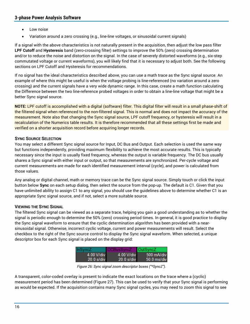
VIEWING THE SYNC SIGNAL The filtered Sync signal can be viewed as a separate trace, helping you gain a good understanding as to whether the signal is periodic enough to determine the 50% (zero) crossing period times. In general, it is good practice to display the Sync signal waveform to ensure that the cyclic determination algorithm has been provided with a near-sinusoidal signal. Otherwise, incorrect cyclic voltage, current and power measurements will result. Select the checkbox to the right of the Sync source control to display the Sync signal waveform. When selected, a unique descriptor box for each Sync signal is placed on the display grid:
Figure 26: Sync signal zoom descriptor boxes (“*SyncZ”).
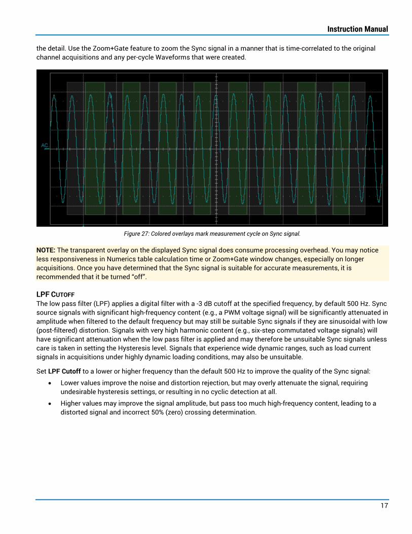
A transparent, color-coded overlay is present to indicate the exact locations on the trace where a (cyclic) measurement period has been determined (Figure 27). This can be used to verify that your Sync signal is performing as would be expected. If the acquisition contains many Sync signal cycles, you may need to zoom this signal to see
Instruction Manual
17
the detail. Use the Zoom+Gate feature to zoom the Sync signal in a manner that is time-correlated to the original channel acquisitions and any per-cycle Waveforms that were created.
Figure 27: Colored overlays mark measurement cycle on Sync signal.
NOTE: The transparent overlay on the displayed Sync signal does consume processing overhead. You may notice less responsiveness in Numerics table calculation time or Zoom+Gate window changes, especially on longer acquisitions. Once you have determined that the Sync signal is suitable for accurate measurements, it is recommended that it be turned “off”.
LPF CUTOFF The low pass filter (LPF) applies a digital filter with a -3 dB cutoff at the specified frequency, by default 500 Hz. Sync source signals with significant high-frequency content (e.g., a PWM voltage signal) will be significantly attenuated in amplitude when filtered to the default frequency but may still be suitable Sync signals if they are sinusoidal with low (post-filtered) distortion. Signals with very high harmonic content (e.g., six-step commutated voltage signals) will have significant attenuation when the low pass filter is applied and may therefore be unsuitable Sync signals unless care is taken in setting the Hysteresis level. Signals that experience wide dynamic ranges, such as load current signals in acquisitions under highly dynamic loading conditions, may also be unsuitable.
Set LPF Cutoff to a lower or higher frequency than the default 500 Hz to improve the quality of the Sync signal:
• Lower values improve the noise and distortion rejection, but may overly attenuate the signal, requiring undesirable hysteresis settings, or resulting in no cyclic detection at all.
• Higher values may improve the signal amplitude, but pass too much high-frequency content, leading to a distorted signal and incorrect 50% (zero) crossing determination.

3-phase Power Analysis Software
18
In Figure 28 we see a capture of a sine-modulated line-line output voltage waveform (Z1, or the Zoom of C1, which is not shown) and the corresponding output line current waveform (Z4, or the zoom of C4, which is not shown). The InSyncZ signal (upper right, based on the zoomed and filtered filtered C1 line-line voltage waveform) and OutSyncZ signal (lower right, based on zoomed and filtered C4 line current waveform) are displayed with the default 500 Hz LPF cutoff.
Figure 28: Sinusoidal Sync signals displayed with default 500 Hz LPF Cutoff.
NOTE: Only one Sync signal is required for proper measurements. Two Sync signals are shown in these examples only to illustrate the difference between using a voltage or current signal for the Sync, and the effects of different LPF Cutoff filter or Hysteresis band settings.
The voltage signal is significantly attenuated in amplitude when filtered (upper right), but still suitable as a Sync signal with the default 100 mdiv hysteresis setting. The current signal (lower right) is an ideal Sync signal since it is highly sinusoidal with high amplitude and fast slew rates, before (and after) filtering.
NOTE: Highly distorted waveforms (e.g., six-step commutated voltage and current waveforms) might require significantly lower LPF cutoff settings than provided by the default 500 Hz setting. See Figure 29.
Instruction Manual
19
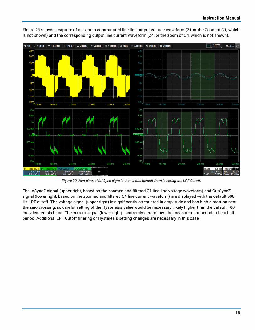
Figure 29 shows a capture of a six-step commutated line-line output voltage waveform (Z1 or the Zoom of C1, which is not shown) and the corresponding output line current waveform (Z4, or the zoom of C4, which is not shown).
Figure 29: Non-sinusoidal Sync signals that would benefit from lowering the LPF Cutoff.
The InSyncZ signal (upper right, based on the zoomed and filtered C1 line-line voltage waveform) and OutSyncZ signal (lower right, based on the zoomed and filtered C4 line current waveform) are displayed with the default 500 Hz LPF cutoff. The voltage signal (upper right) is significantly attenuated in amplitude and has high distortion near the zero crossing, so careful setting of the Hysteresis value would be necessary, likely higher than the default 100 mdiv hysteresis band. The current signal (lower right) incorrectly determines the measurement period to be a half period. Additional LPF Cutoff filtering or Hysteresis setting changes are necessary in this case.

3-phase Power Analysis Software
20
Figure 30 shows the same Sync signals with an LPF Cutoff filter setting of 100 Hz (as opposed to the 500 Hz used in Figure 29).
Figure 30: Non-sinusoidal Sync signals corrected by adjusting LPF Cutoff filter.
HYSTERESIS BAND The Hysteresis band setting defines an amplitude “band” that the Sync signal must exceed before the signal slope will be determined to be acceptable for use in the 50% (zero) crossing determination. The default value is 100 millidivisions (mdiv), with the unit “divisions” being equal to oscilloscope vertical grid divisions.
• Lower hysteresis values improve the ability to detect a 50% (zero) crossing on a smaller amplitude signals, but with risk that false 50% (zero) crossings will be detected.
• Higher hysteresis values lessen the impact of signal distortion or noise in determination of the 50% (zero) crossing, but with risk of reduced accuracy of 50% (zero) crossing detection.
Some non-zero hysteresis value is required to prevent false 50% (zero) crossing determinations. However, this also means that the Sync signal must meet a minimum amplitude requirement, and be relatively noise free at lower amplitudes. Signals with very wide dynamic ranges and very high distortion (e.g. a six-step commutated current signal with very high dynamic range) are therefore likely to make bad Sync signals, since the low amplitude portions of the Sync waveform might be smaller than the hysteresis setting that is required. In this case, it is best to choose a different signal that has a more constant amplitude or a smaller dynamic range.

Instruction Manual
21
To understand how the hysteresis band setting works, consider the example in Figure 31 of a perfect sinusoid. In this case, the zero or 50% crossing level is simple to detect and the measurement intervals are easily determined.
Figure 31: Measurement intervals on monotonic signal.
Now, consider the example in Figure 32 in which there is a non-monotonicity near the zero or 50% crossing level. The non-monotonicity period is detected as a measurement interval, resulting in an incorrect period determination, which will result in incorrect calculations.
Figure 32: Non-monotonic signal produces “false” measurement intervals.
By using the Hysteresis control, you can set a hysteresis band level that is greater than the amplitude of the non-monotonicity and avoid false measurement interval calculations.
Figure 33: Hysteresis Band corrects for non-monotonicity.
3-phase Power Analysis Software
22
ZOOM SYNC SIGNAL On longer acquisitions, especially those with dynamic load conditions, it may be necessary to zoom the Sync signal to verify that a good cyclic determination is achieved. Press the Zoom+Gate button to create new zoom traces of each source waveform, time-correlated to a zoom of the Sync signal. If undesirable results are obtained, adjust LFP cutoff and Hysteresis settings as necessary, or choose a different signal to use as the Sync source. See Zoom+Gate Mode (p.35) for more information.
EXAMPLE SYNC SIGNAL SELECTION – LONG ACQUISITION WITH WIDE DYNAMIC RANGE AND OVERLOAD As described earlier in this section, long acquisitions of signals that have wide dynamic ranges and distortion require care in selecting the Sync signal in order to achieve accurate results.
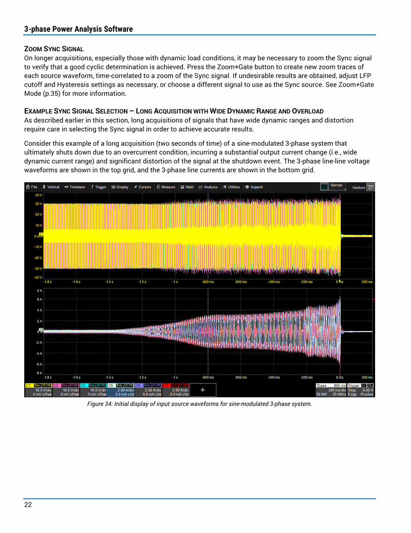
Consider this example of a long acquisition (two seconds of time) of a sine-modulated 3-phase system that ultimately shuts down due to an overcurrent condition, incurring a substantial output current change (i.e., wide dynamic current range) and significant distortion of the signal at the shutdown event. The 3-phase line-line voltage waveforms are shown in the top grid, and the 3-phase line currents are shown in the bottom grid.
Figure 34: Initial display of input source waveforms for sine-modulated 3-phase system.
Instruction Manual
23
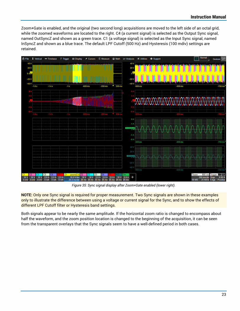
Zoom+Gate is enabled, and the original (two second long) acquisitions are moved to the left side of an octal grid, while the zoomed waveforms are located to the right. C4 (a current signal) is selected as the Output Sync signal, named OutSyncZ and shown as a green trace. C1 (a voltage signal) is selected as the Input Sync signal, named InSyncZ and shown as a blue trace. The default LPF Cutoff (500 Hz) and Hysteresis (100 mdiv) settings are retained.
Figure 35: Sync signal display after Zoom+Gate enabled (lower right).
NOTE: Only one Sync signal is required for proper measurement. Two Sync signals are shown in these examples only to illustrate the difference between using a voltage or current signal for the Sync, and to show the effects of different LPF Cutoff filter or Hysteresis band settings.
Both signals appear to be nearly the same amplitude. If the horizontal zoom ratio is changed to encompass about half the waveform, and the zoom position location is changed to the beginning of the acquisition, it can be seen from the transparent overlays that the Sync signals seem to have a well-defined period in both cases.

3-phase Power Analysis Software
24
Now, if the zoom position is changed to the end of the acquisition, as in Figure 36, it can be seen that near the end of the acquisition (where the overload condition is occurring), the voltage and current signals have different behaviors despite the identical LPF Cutoff and Hysteresis settings, but neither of them achieve a good period determination in this location.
Figure 36: Changing zoom position changes display of all zoomed waveforms, including Sync signals.

Instruction Manual
25
Adjusting LPF Cutoff to 160 Hz and Hysteresis to 20 mdiv on both Sync signals shows that the C4 current signal (green trace, used for OutSyncZ) provides a better measurement interval for both current and voltage signals.
Figure 37: Adjusting filters reveals OutSyncZ can be a good choice Sync signal.

3-phase Power Analysis Software
26
However, a zoom to the beginning of the acquisition shows that proper period determination at the beginning of the acquisition is better achieved using the C1 line-line voltage signal (the source of InSyncZ).
Figure 38: Zooming to the beginning of the acquisition shows InSyncZ is actually the best choice Sync signal.

Instruction Manual
27
EXAMPLE SYNC SIGNAL SELECTION – USING A DIGITAL SIGNAL CORRESPONDING TO THE DEVICE SWITCHING PERIOD The device switching period, measured either with an analog or digital (Mixed Signal) input channel, may be used as a Sync signal. In the example below, it was required to calculate power for each switching period to understand the operation of a control system that dynamically changed the magnetic flux of a permanent magnet motor rotor. The switching period was measured by C8 (orange, lower left), and the sync periods were calculated correctly using a high frequency LPF cutoff setting (1 MHz) and 400 mdiv of hysteresis.
Figure 39: Device switching period used as Sync signal.

3-phase Power Analysis Software
28
DC Bus Dialog To correctly calculate power values, identify the wiring configuration used by the DC Bus power section and assign input sources to each voltage. Choose from either:
• 1-phase-2-wire (1V1A)
• None–which de-activates any input assignments on the dialog
Input assignments are performed the same as for the Input and Output sections, as is the Sync signal selection and adjustment. See the previous topics on Voltage and Current Assignments, Sync Signal, and Zoom+Gate for instructions on using these controls.
The DC Bus Sync signal source can be the same as or different than that selected for Input and Output. However, we recommend using the same Sync Signal as one of these, since DC Bus signals are non-periodic, and measurement intervals must be made consistent with the Input or Output measurement intervals.
Figure 40: DC Bus setup dialog.
Instruction Manual
29
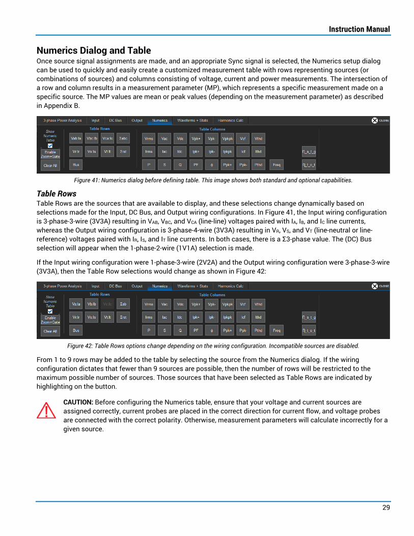
Numerics Dialog and Table Once source signal assignments are made, and an appropriate Sync signal is selected, the Numerics setup dialog can be used to quickly and easily create a customized measurement table with rows representing sources (or combinations of sources) and columns consisting of voltage, current and power measurements. The intersection of a row and column results in a measurement parameter (MP), which represents a specific measurement made on a specific source. The MP values are mean or peak values (depending on the measurement parameter) as described in Appendix B.
Figure 41: Numerics dialog before defining table. This image shows both standard and optional capabilities.
Table Rows Table Rows are the sources that are available to display, and these selections change dynamically based on selections made for the Input, DC Bus, and Output wiring configurations. In Figure 41, the Input wiring configuration is 3-phase-3-wire (3V3A) resulting in VAB, VBC, and VCA (line-line) voltages paired with IA, IB, and IC line currents, whereas the Output wiring configuration is 3-phase-4-wire (3V3A) resulting in VR, VS, and VT (line-neutral or line-reference) voltages paired with IR, IS, and IT line currents. In both cases, there is a Σ3-phase value. The (DC) Bus selection will appear when the 1-phase-2-wire (1V1A) selection is made.
If the Input wiring configuration were 1-phase-3-wire (2V2A) and the Output wiring configuration were 3-phase-3-wire (3V3A), then the Table Row selections would change as shown in Figure 42:
Figure 42: Table Rows options change depending on the wiring configuration. Incompatible sources are disabled.
From 1 to 9 rows may be added to the table by selecting the source from the Numerics dialog. If the wiring configuration dictates that fewer than 9 sources are possible, then the number of rows will be restricted to the maximum possible number of sources. Those sources that have been selected as Table Rows are indicated by highlighting on the button.
CAUTION: Before configuring the Numerics table, ensure that your voltage and current sources are assigned correctly, current probes are placed in the correct direction for current flow, and voltage probes are connected with the correct polarity. Otherwise, measurement parameters will calculate incorrectly for a given source.
3-phase Power Analysis Software
30
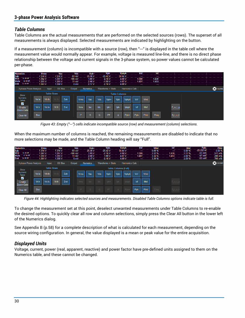
Table Columns Table Columns are the actual measurements that are performed on the selected sources (rows). The superset of all measurements is always displayed. Selected measurements are indicated by highlighting on the button.
If a measurement (column) is incompatible with a source (row), then “---“ is displayed in the table cell where the measurement value would normally appear. For example, voltage is measured line-line, and there is no direct phase relationship between the voltage and current signals in the 3-phase system, so power values cannot be calculated per-phase.
Figure 43: Empty (“---“) cells indicate incompatible source (row) and measurement (column) selections.
When the maximum number of columns is reached, the remaining measurements are disabled to indicate that no more selections may be made, and the Table Column heading will say “Full”.
Figure 44: Highlighting indicates selected sources and measurements. Disabled Table Columns options indicate table is full.
To change the measurement set at this point, deselect unwanted measurements under Table Columns to re-enable the desired options. To quickly clear all row and column selections, simply press the Clear All button in the lower left of the Numerics dialog.
See Appendix B (p.58) for a complete description of what is calculated for each measurement, depending on the source wiring configuration. In general, the value displayed is a mean or peak value for the entire acquisition.
Displayed Units Voltage, current, power (real, apparent, reactive) and power factor have pre-defined units assigned to them on the Numerics table, and these cannot be changed.

Instruction Manual
31
Creating Per-Cycle Waveforms from the Numerics Table The Numerics table is interactive. Touching or clicking a table cell creates a new, per-cycle Waveform of that MP.
A per-cycle Waveform is a synthesized waveform tracking the per-cycle MP values versus time, time-correlated to the original acquisition waveforms. When displayed, the waveform has a unique color and descriptor box showing the waveform name (e.g., P(Σrst)) and vertical and horizontal scale information. The per-cycle Waveform may be used as the source of a zoom, math function, measurement parameter, memory, etc. using the standard Teledyne LeCroy oscilloscope tools.
Figure 45: Numerics table cells indicate which motor parameters have per-cycle Waveforms.
When an MP has a per-cycle Waveform displayed, the color of the corresponding Numerics table cell will change, as shown in Figure 45.
The default location for new per-cycle Waveforms is Grid 1 (Grid 1 of Tab1 if in Q-Scape display mode); from there they may be moved to any desired grid, just like any other trace.
To turn off the synthesized per-cycle Waveform, simply touch or click the Numerics table cell again, and the trace is removed from the display, the same as if you had turned off the waveform by clearing the checkbox on the Waveforms + Stats dialog.

3-phase Power Analysis Software
32
Waveforms + Stats Dialog and Statistics Table The Waveforms + Stats dialog provides a summary of the MPs and per-cycle Waveforms, as well as alternative methods for creating and modifying them.
Per-cycle Waveforms
When a per-cycle Waveform is created, statistical information is displayed in the Statistics table below the Numerics table, and a corresponding descriptor box appears below the grid.
Figure 46: Per-cycle Waveform descriptor boxes.
Selecting the descriptor box activates that trace and the following Waveform Vertical Scale Settings on the Waveforms + Stats dialog.
Height/div or the arrow buttons adjusts the trace amplitude.
Center shifts its horizontal position so it is centered on the grid.
Find Scale automatically detects and sets the scale based on waveform mean amplitude.
Auto Find Scale checkbox indicates whether a new scale should be found automatically whenever the values change enough to warrant it a scale change.
Figure 47: Synthesized per-cycle Waveform vertical scale settings.
By definition, per-cycle Waveforms don’t have horizontal rescale capability and are always locked to the same timebase setting as the original source traces, or to the zoom scale when Zoom+Gate is enabled. However, if desired, you can create a zoom trace of the per-cycle Waveform using the standard zoom controls, which can be adjusted horizontally.
TIP: If using the Zoom math function, select the per-cycle Waveform by name (e.g., φ(Σrst)) from the “Other” category on the Select Source pop-up dialog. These selections automatically change depending on the MP setup. NOTE: When a per-cycle Waveform is zoomed, the source shown on the zoom descriptor box will be TPnn, with nn being the MP number that corresponds to the waveform.

Instruction Manual
33
Statistics Table When a per-cycle Waveform is created, a column for that MP is added to the Statistics table. While the Numerics table displays the latest per-cycle values of an MP, the values in the Statistics table are the statistical data values that comprise the per-cycle Waveform. Thus, if there are 17 unique measurement periods in the acquisition (and 17 MP values), the Statistics table will provide the statistical mean, minimum, maximum, standard deviation, and number of measurements calculated, as shown in Figure 48.
Figure 48: Statistics table display.
The definition of the values displayed is as follows:
• Value = last value calculated in the acquisition set
• Mean = mean value for all “N” values in the statistical set
• Min = minimum value for all “N” values in the statistical set
• Max = maximum value for all “N” values in the statistical set
• Sdev = standard deviation value for all “N” values in the statistical set
• Num = number of values in the statistical set
• Status = indication that the measurement was performed correctly or not
You can show or hide this table by selecting/deselecting the Show Statistics Table checkbox on the Waveforms + Stats dialog.
If desired, the per-cycle Waveform can be hidden while retaining the MP in the Statistics table by clearing the Waveform checkbox next to the MP.
To quickly empty the Statistics table, touch the Clear All button at the bottom left of the Waveform + Stats dialog.
3-phase Power Analysis Software
34
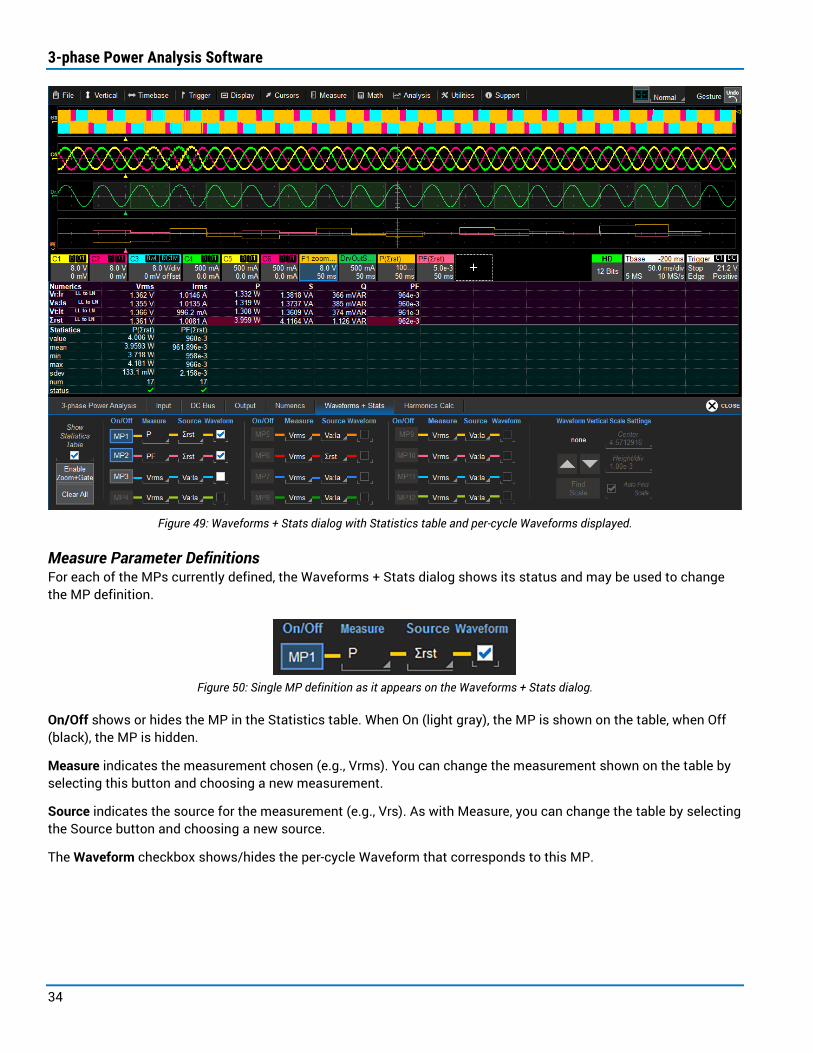
Figure 49: Waveforms + Stats dialog with Statistics table and per-cycle Waveforms displayed.
Measure Parameter Definitions For each of the MPs currently defined, the Waveforms + Stats dialog shows its status and may be used to change the MP definition.
Figure 50: Single MP definition as it appears on the Waveforms + Stats dialog.
On/Off shows or hides the MP in the Statistics table. When On (light gray), the MP is shown on the table, when Off (black), the MP is hidden.
Measure indicates the measurement chosen (e.g., Vrms). You can change the measurement shown on the table by selecting this button and choosing a new measurement.
Source indicates the source for the measurement (e.g., Vrs). As with Measure, you can change the table by selecting the Source button and choosing a new source.
The Waveform checkbox shows/hides the per-cycle Waveform that corresponds to this MP.

Instruction Manual
35
Zoom+Gate Mode The Zoom+Gate feature provides a simple method for zooming all input sources (analog and digital), per-cycle Waveforms and Sync signals together, positioning the zoom window on any portion of the trace. The common zoom window then acts as the measurement gate for the Numerics and Statistics tables. Thus, it is possible to push one button (Zoom+Gate), turn a couple of knobs to adjust zoom ratio and position, and quickly compare the acquired waveforms to the per-cycle Waveforms, while automatically and instantly recalculating the measurements for only the zoomed area.
Accessing Zoom+Gate Touching the Enable Zoom+Gate button on the Input, DC Bus or Output dialogs will do the following:
• Create new zoom traces (Zn) of all displayed input sources.
TIP: These new Zn waveforms will likely not be located in the grid you desire, so select a new grid style and/or drag the trace descriptor boxes to different grids to position them appropriately.
• Add all Zn traces to a multi-zoom group so that they are zoomed with the same ratio and positioned in a time-correlated fashion.
• Include any per-cycle Waveforms and Sync signal traces in the multi-zoom with the Zn traces so that all are zoomed and positioned in a time-correlated fashion.
Any new per-cycle Waveforms and Sync signals that are created after Zoom+Gate is enabled are automatically added to the multi-zoom group to maintain the time-correlation of all signals.
Other math (Fn) or memory (Mn) traces may also be added to the Zoom+Gate group, as desired. From the menu bar, select Math > Zoom Setup, then on the MultiZoom tab, include the additional Fn or Mn traces in the multi-zoom group.
When Zoom+Gate is enabled, the Enable Zoom+Gate “button” is highlighted light gray. The front panel Zoom button is also lit, indicating that the Vertical and Horizontal knobs may be used to control the zoom ratio and position, and thus also control the gating location and size.
NOTE: Using the front panel Zoom button to turn off zooms also de-activates Zoom+Gate.
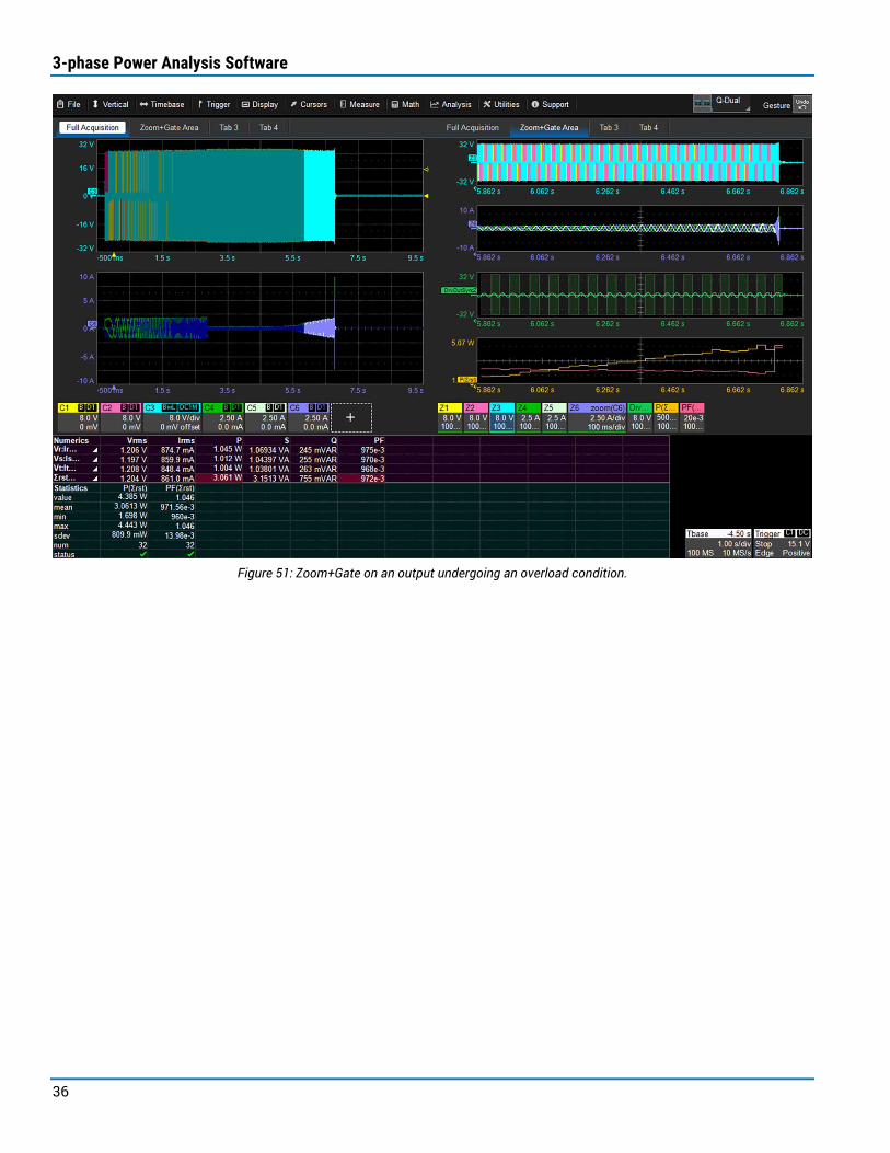
Zoom+Gate Example In this example, system Output is acquired, and MPs are calculated in the Numerics table, while several per-cycle Waveforms are created and shown on the Statistics table. The current signal undergoes a wide dynamic range—it is not necessarily the best Sync signal—so the voltage signal is chosen instead and appropriately filtered with a Hysteresis band setting of 500 mdiv to avoid bad cyclic calculations. Nonetheless, the overload condition just before shutdown shows a lot of ringing, making it difficult to determine cyclic values in this area.
Zoom+Gate is enabled to create new zoom traces of each of the inputs and the per-cycle Waveforms. The Q-Dual display mode is used to show the full acquisition traces on the left and the Zoom+Gate traces on the right.
The stress on the system as it reaches overload conditions can be seen in the zoomed voltage and current waveforms. The P(SumRST) and PF(SumRST) Waveforms show the Power and Power Factor values during the overload, which are represented in the Statistics table. The Statistics table indicates that the Zoom+Gate area has a total of 16 measurement cycles (you can count the cycles on the zoomed OutSync waveform).
3-phase Power Analysis Software
36
Figure 51: Zoom+Gate on an output undergoing an overload condition.

Instruction Manual
37
Harmonics Calculation Option Harmonics Calculation is an optional software package for use with the 3-phase Power Analysis software. It adds the following capabilities to the standard tools:
• Advanced harmonic filtering of Input and Output for voltage, current, and power measurements
• Total Harmonic Distortion (THD) measurement parameters for voltage, current, and power
• A Harmonic Calc(ulations) tab for setting up per-order harmonic measurements, which are displayed in a new Harmonic Order table
• Spectral waveform displays
Harmonics Calculation Overview The 3-phase Power Analysis software includes standard capabilities to filter Numerics table measurements to include all acquired harmonics (Full Spectrum) or only the Fundamental. However, it can be helpful to more precisely limit the harmonic content of the acquired waveforms when calculating Numerics table MPs. The Harmonics Calculation option provides a method to harmonically filter input waveforms using either:
• Fundamental+N―a user-defined number (N) of harmonics from the fundamental to include in the Numerics table calculations.
• Range―a user-defined starting point for the range other than the fundamental, including the ability to filter to a single harmonic order.
Additionally, the Harmonics Calculation option provides per-order harmonic measurement results for up-to-nine waveforms: voltage, current, and power for each phase of a 3-phase system. The method used allows for both steady-state (Fixed Frequency) and dynamic (Varying Frequency) operating conditions. The steady-state method is similar to that found in a typical power analyzer. The dynamic method provides maximum flexibility for variable frequency outputs. This is made possible by a flexible, per-cycle period detection technique far more advanced than what is typically found in power analyzers, which can only perform steady-state harmonic analysis.
Lastly, per-cycle THD measurement parameters for voltage, current and power may be included in the Numerics table display. Per-cycle synthesized waveforms for THD can be created simply by touching a THD measurement parameter cell in the Numerics table.
NOTE: Regardless of the acquisition sample rate used to acquire the voltage and current waveforms, the 3-phase Power Analysis uses intelligent algorithms to reduce the number of samples utilized for the harmonics calculations for both the Harmonics Filters (in the Input and Output setup dialogs), the Harmonics (per-order) Calculations, and the THD Numerics calculations. At a minimum, the sample rate should be at least ten times the switching frequency of a pulse-width-modulated signal, with appreciably more sample rate used if non-harmonic behaviors are also to be investigated at the same time. If the acquired voltage and current waveforms are highly oversampled, there number of points used in the various harmonic calculations will be automatically reduced.
Also note that calculations are done on a per-cycle basis, and processing time will increase when there are many cyclic periods within an acquisition. Gain experience first using acquisitions with fewer cyclic periods to understand the processing time required for these complex calculations. Then, increase the acquisition length to acquire more cyclic periods once the processing time tradeoffs are well understood.

3-phase Power Analysis Software
38
Harmonic Filtering – Input and Output Dialogs The Harmonics Calculation option activates the (normally disabled) Fundamental+N and Range Harmonic Filter selections on the Input and Output setup dialogs. The Harmonic Filter is used to calculate the measurement results shown in the Numerics table. (This filter selection is not used for the Harmonic Order table measurements, which are set up separately as explained on p.41.)
Figure 52: Harmonic Filter controls.
The Fundamental, Fundamental+N, and Range Harmonic Filter selections perform a mathematical operation on the acquired voltage and current waveforms using a Discrete Fourier Transform (DFT). This mathematical operation transforms the acquired waveform sample points to the frequency domain for each cyclic period calculated from the Sync source signal. For each cyclic period, there is a unique DFT, and therefore typically multiple DFTs per acquisition. For each DFT, the inverse of the cyclic period is defined to be the Fundamental frequency, and integer multiples of the Fundamental are the harmonic orders. The total frequency content of the DFT is then "binned" into the various harmonic orders.
The Harmonic Filter selection is the user input to this calculation, determining the relevant harmonic orders. Based on this setting, unwanted harmonic orders are discarded from the DFT, while desired harmonic orders are retained. An inverse DFT is then performed on each DFT to convert the remaining frequency-domain waveform back to a time domain waveform that represents only the desired harmonic orders. The process is repeated for each cyclic period for all acquired voltage and current waveforms, using the harmonically filtered waveforms to calculate the measurement results shown in the Numerics table. This technique works on waveforms with constant or highly variable cyclic periods.
NOTE: Although used for Numerics table calculations, the harmonically filtered waveforms are not displayed, and the originally acquired channel waveforms remain the same.
An example of what the harmonic filter does is shown in Figure 53 and Figure 54. The images show a width-modulated waveform (thick red trace) that is not harmonically filtered. This waveform is made up of many
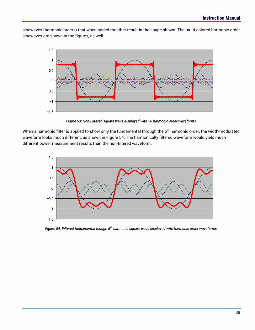
Instruction Manual
39
sinewaves (harmonic orders) that when added together result in the shape shown. The multi-colored harmonic order sinewaves are shown in the figures, as well.
Figure 53: Non-Filtered square wave displayed with 50 harmonic order waveforms.
When a harmonic filter is applied to show only the fundamental through the 5th harmonic order, the width-modulated waveform looks much different, as shown in Figure 54. The harmonically filtered waveform would yield much different power measurement results than the non-filtered waveform.
Figure 54: Filtered fundamental though 5th harmonic square wave displayed with harmonic order waveforms.
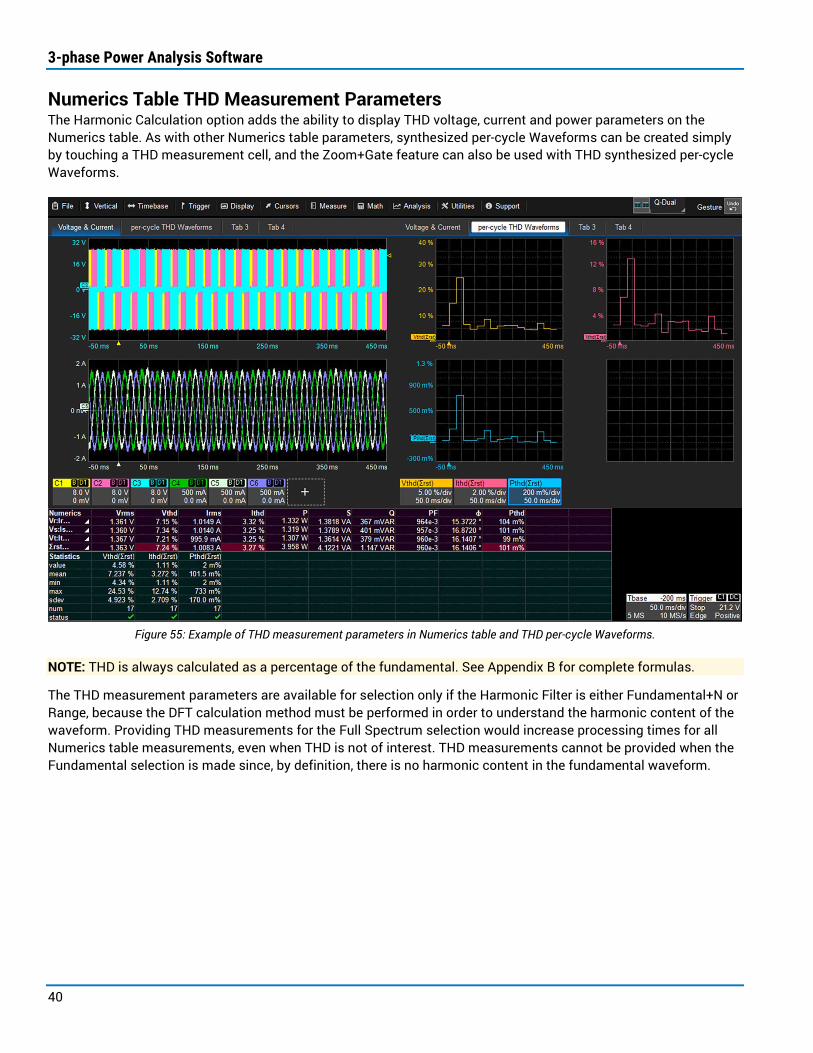
3-phase Power Analysis Software
40
Numerics Table THD Measurement Parameters The Harmonic Calculation option adds the ability to display THD voltage, current and power parameters on the Numerics table. As with other Numerics table parameters, synthesized per-cycle Waveforms can be created simply by touching a THD measurement cell, and the Zoom+Gate feature can also be used with THD synthesized per-cycle Waveforms.
Figure 55: Example of THD measurement parameters in Numerics table and THD per-cycle Waveforms.
NOTE: THD is always calculated as a percentage of the fundamental. See Appendix B for complete formulas.
The THD measurement parameters are available for selection only if the Harmonic Filter is either Fundamental+N or Range, because the DFT calculation method must be performed in order to understand the harmonic content of the waveform. Providing THD measurements for the Full Spectrum selection would increase processing times for all Numerics table measurements, even when THD is not of interest. THD measurements cannot be provided when the Fundamental selection is made since, by definition, there is no harmonic content in the fundamental waveform.

Instruction Manual
41
Harmonics Calc Setup Dialog Once the proper voltage and current signal assignments have been made on the Input or Output dialogs, the Harmonics Order table may be set up and displayed using the Harmonics Calc(ulation) dialog. These harmonic calculations can be performed on any phase of either the Input or Output voltage, current and power waveforms. Spectral waveforms showing the result of the selected calculations are displayed, along with harmonic order measurement values in a new Harmonic Order table.
Figure 56: Harmonics Calc setup dialog for Varying Frequency Detection Mode.
Harmonics Calc Setup and Fundamental Frequency Detection
Figure 57: Harmonics Calc Setup and Fundamental Frequency Detection controls.
Enter the Num(ber) of Harmonics orders of interest to be measured. This setting determines measurements from the fundamental to the Nth harmonic.
NOTE: This is different from the Harmonic Filter setting on the Input and Output dialogs, which only applies to the Numerics table measurements. The Num of Harmonics setting is only used to calculate results in the Harmonics Order table.
Under Fundamental Frequency Detection, choose the method for detecting the fundamental frequency:
• Fixed Frequency allows the Num(ber) of Harmonics to be set up to 100, but does not allow the use of the Zoom+Gate feature. It only calculates harmonics for voltage and current waveforms. By default, the input current signal is used to Auto Detect the frequency, but you may enter a User Defined base frequency as an alternative to using the input current signal frequency.
• Varying Frequency uses the Sync signal defined for the Input or Output to determine the proper period of each cycle. The Num(ber) of Harmonics is limited to 50 with this setting, and the harmonic calculations are done on a per-cycle basis. It calculates harmonics for voltage, current and power waveforms. Since the harmonics are calculated per-cycle, the processing times may be significantly longer when compared to the fixed frequency mode. However, the Varying Frequency method can be used with the Zoom+Gate feature.
The Fixed Frequency setting should only be used with a fixed frequency input, such as a 50/60 Hz Input or a Variable Frequency Output operating under steady-state conditions that result in a steady-state frequency (fixed, but not necessarily 50 or 60 Hz) during the entire acquisition. In both cases, the average frequency throughout the entire
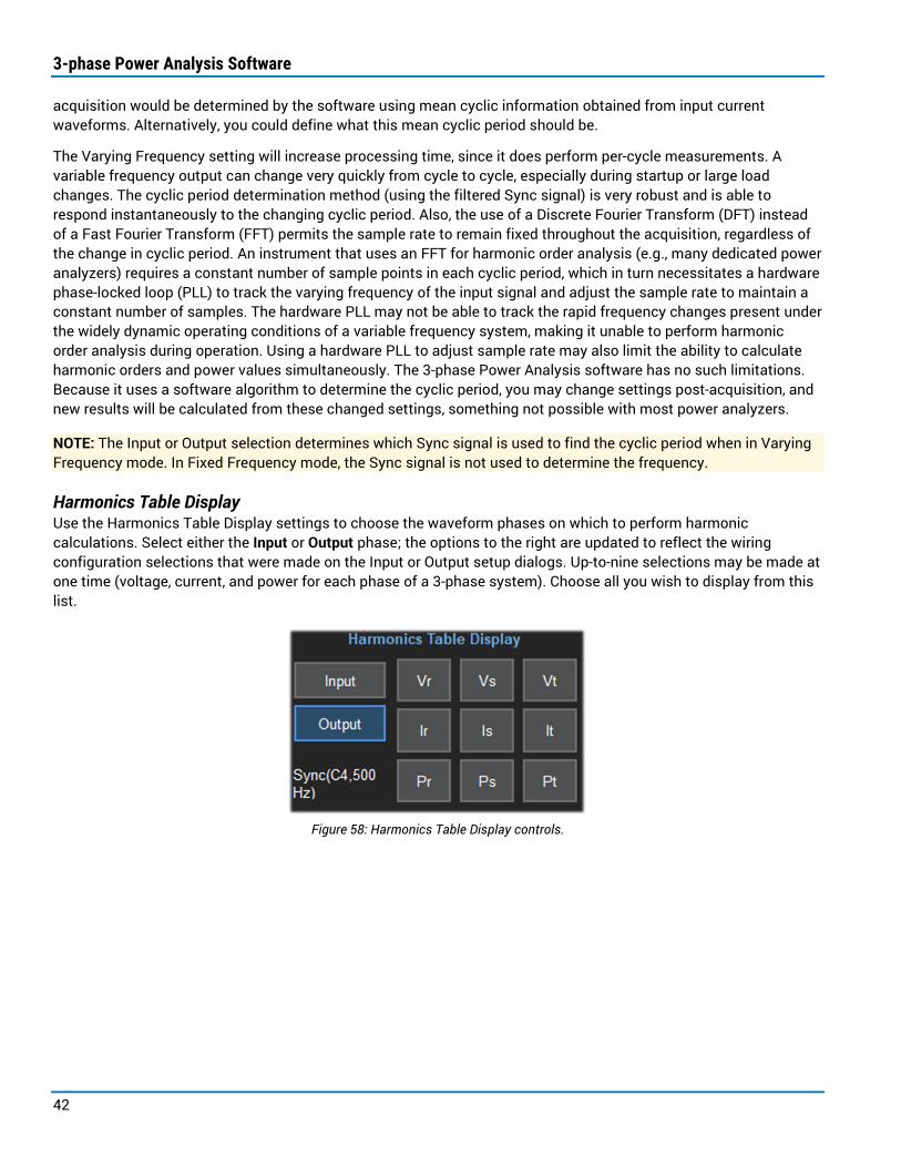
3-phase Power Analysis Software
42
acquisition would be determined by the software using mean cyclic information obtained from input current waveforms. Alternatively, you could define what this mean cyclic period should be.
The Varying Frequency setting will increase processing time, since it does perform per-cycle measurements. A variable frequency output can change very quickly from cycle to cycle, especially during startup or large load changes. The cyclic period determination method (using the filtered Sync signal) is very robust and is able to respond instantaneously to the changing cyclic period. Also, the use of a Discrete Fourier Transform (DFT) instead of a Fast Fourier Transform (FFT) permits the sample rate to remain fixed throughout the acquisition, regardless of the change in cyclic period. An instrument that uses an FFT for harmonic order analysis (e.g., many dedicated power analyzers) requires a constant number of sample points in each cyclic period, which in turn necessitates a hardware phase-locked loop (PLL) to track the varying frequency of the input signal and adjust the sample rate to maintain a constant number of samples. The hardware PLL may not be able to track the rapid frequency changes present under the widely dynamic operating conditions of a variable frequency system, making it unable to perform harmonic order analysis during operation. Using a hardware PLL to adjust sample rate may also limit the ability to calculate harmonic orders and power values simultaneously. The 3-phase Power Analysis software has no such limitations. Because it uses a software algorithm to determine the cyclic period, you may change settings post-acquisition, and new results will be calculated from these changed settings, something not possible with most power analyzers.
NOTE: The Input or Output selection determines which Sync signal is used to find the cyclic period when in Varying Frequency mode. In Fixed Frequency mode, the Sync signal is not used to determine the frequency.
Harmonics Table Display Use the Harmonics Table Display settings to choose the waveform phases on which to perform harmonic calculations. Select either the Input or Output phase; the options to the right are updated to reflect the wiring configuration selections that were made on the Input or Output setup dialogs. Up-to-nine selections may be made at one time (voltage, current, and power for each phase of a 3-phase system). Choose all you wish to display from this list.
Figure 58: Harmonics Table Display controls.

Instruction Manual
43
Units/Limits Choose the Unit in which to display harmonics calculation results: Amperes (A), Volts (V), Watts (W), percent (%), or decibels (dB). When using percent, THD results are given as a percentage of the fundamental component.
𝑇𝑇𝑇𝑇𝑇𝑇% = 𝐸𝐸𝐸𝐸𝐸𝐸ℎ ℎ𝐸𝐸𝑎𝑎𝑎𝑎𝑎𝑎𝑎𝑎𝑎𝑎𝐸𝐸 𝑎𝑎𝑎𝑎𝑜𝑜𝑜𝑜𝑎𝑎
𝐹𝐹𝐹𝐹𝑎𝑎𝑜𝑜𝐸𝐸𝑎𝑎𝑜𝑜𝑎𝑎𝐹𝐹𝐸𝐸𝐹𝐹 𝐸𝐸𝑎𝑎𝑎𝑎𝑐𝑐𝑎𝑎𝑎𝑎𝑜𝑜𝑎𝑎𝐹𝐹𝑥𝑥 100
In Fixed Frequency mode, you may optionally compare the measured current harmonics to the limits set by the IEC 61000 Class A specifications. Convenient Pass/Fail indicators are posted next to the measured current values in the Harmonics Order table.
Figure 59: Units/Limits controls.
Alternatively, you may compare to a Custom limit set. When using this option, Browse to and select your user-defined Limit File.
Limits are defined in a .txt file in the format shown in Figure 60. The first column represents the harmonic order. The second column (separated by a tab from the first column) represents the current limit in Amps, or in percent if using percent as the unit. If the unit is decibels, enter the current limit in Amps in the limits file, and it will be converted to dBµA automatically.
Figure 60: Example custom harmonic limits file.

3-phase Power Analysis Software
44
Spectrum Zoom A Spectral waveform is displayed for each input waveform selected under Harmonics Table Display. Each Spectral waveform may be zoomed independently. As the Spectrum Zoom controls can only control one Spectral waveform at a time, first activate the waveform of interest by selecting its descriptor box (Spec**).
TIP: The active Spectral waveform is shown next to the Vertical Spectrum Zoom controls.
Figure 61: Spectrum Zoom controls.
Harmonics Order Table The Harmonics Order table is an additional display only available with the Harmonics Calculation option. It is separate from the standard Numerics table. The values displayed are always presented as Line-Neutral or Line-Reference values. If the signals are probed Line-Line, a Line-Line to Line-Neutral conversion is automatically performed to calculate the values for this table. Figure 62 shows an example Harmonics Order table display when the Fixed Frequency method of Fundamental Frequency Detection is used.
Figure 62: Fixed Frequency Harmonics Order table.
NOTE: A Pass/Fail test may be applied when the Fixed Frequency method is used. Limits appear in the Limit[%] column and results in the Pass/Fail column. However, Power Harmonics cannot be calculated with this method.
Figure 63 shows an example Harmonics Order table display when the Varying Frequency method of Fundamental Frequency Detection is used. This table does not have a Freq [Hz] column for each Harmonic order since, by definition, the frequency is varying.
In both cases, the measurement values in the Harmonics Order table are “per-order”, but not per-cycle–they are the mean value for all the cycles.

Instruction Manual
45
Figure 63: Varying Frequency Harmonics Order table and Spectral waveform display.
You cannot generate a per-cycle Waveform by selecting an individual cell of the Harmonics Order table as you can with the Numerics table (as the Harmonics Order table displays the mean value for each order). If a per-cycle Waveform is required, do the following to generate it:
1. Use the Range harmonics filter in either the Input or Output setup, choosing a range that covers one harmonic order (i.e., from 3 to 3 for harmonic order 3).
2. Turn on the THD measurement parameter on the Numerics tab.
3. Select the cell of interest from the Numerics table to create the per-cycle Waveform for that order.

3-phase Power Analysis Software
46
Spectral Waveform Display Spectral waveforms are displays that contain bars representing the harmonic order value for each harmonic order specified. The Spectral waveforms bin the surrounding frequency components to the harmonic orders, which results in an easy-to-read display, unlike a simple FFT math calculation. These Spectral waveforms vary in thickness based on the number of harmonics specified, giving the appearance of a bar graph as shown in Figure 64.
Figure 64: Spectral waveform display.
Cursors can be placed anywhere on the Spectral waveforms to read out the harmonic order values.
In some cases, the Spectral waveform may have the appearance of gaps within the bars (see Figure 65). This occurs when the specified number of harmonics is low and/or when the display grid is elongated (for example, in Single grid mode).
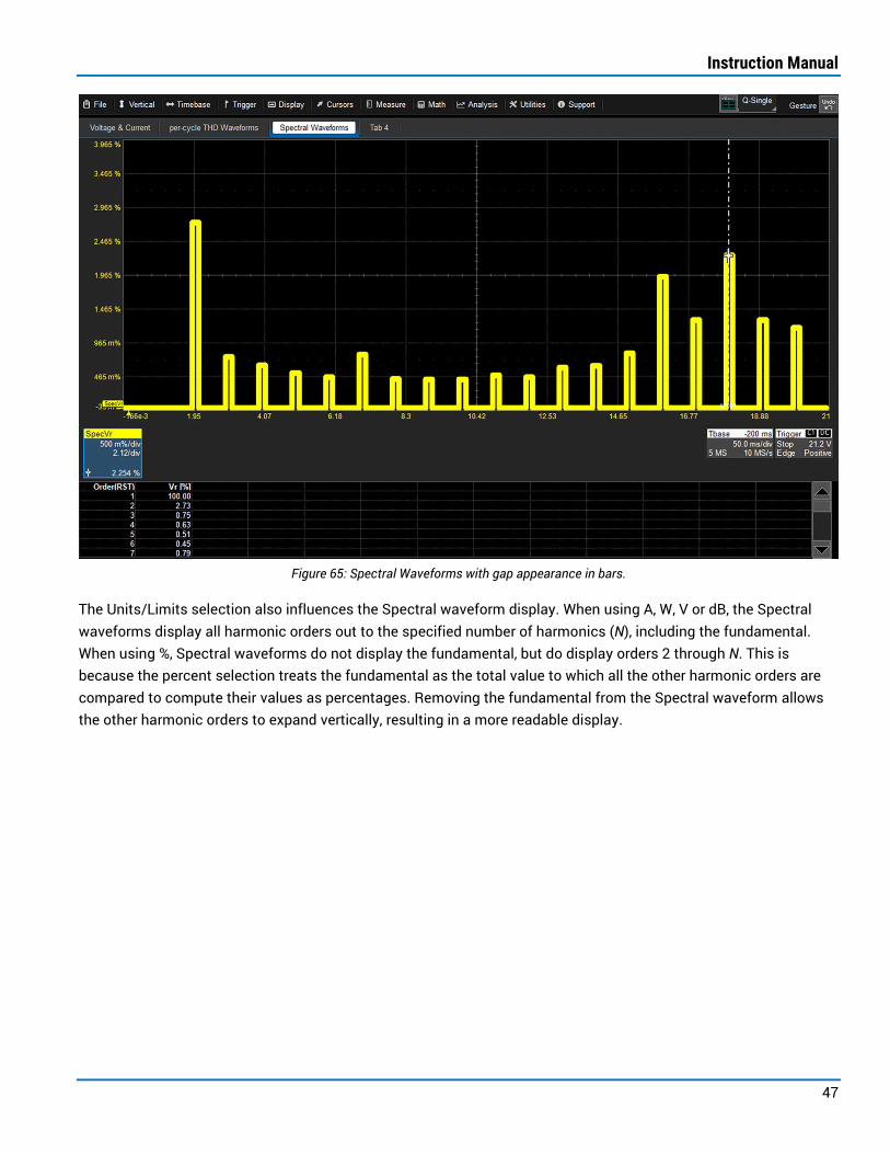
Instruction Manual
47
Figure 65: Spectral Waveforms with gap appearance in bars.
The Units/Limits selection also influences the Spectral waveform display. When using A, W, V or dB, the Spectral waveforms display all harmonic orders out to the specified number of harmonics (N), including the fundamental. When using %, Spectral waveforms do not display the fundamental, but do display orders 2 through N. This is because the percent selection treats the fundamental as the total value to which all the other harmonic orders are compared to compute their values as percentages. Removing the fundamental from the Spectral waveform allows the other harmonic orders to expand vertically, resulting in a more readable display.

3-phase Power Analysis Software
48
Vector Display Option 3-Phase Vector Display is an optional software package for use with the 3-Phase Power Analysis software that adds the ability to generate vector plots of the Input or the Output to the standard application. Both Input and Output plots can be displayed together, each appropriately labelled according to the phases represented (e.g., R, S and T for output).
The vector display reflects (a) magnitudes of voltage and current vectors, (b) angle between them and (c) relative position of the V/I of one phase with respect to the other phases.
All vector display magnitude and angle values, by default, are identical to the values in the Numerics table. If the Zoom + Gate feature is turned on, the plots are calculated on the zoomed waveforms, just as the Numerics table measurements are now calculated on those waveforms. Any change to the zoom position or ratio will cause the vector plots to update automatically.
You can select to calculate the vector display magnitude and angle values according to a vector average by selecting the Vector Average checkbox (see below). When Vector Average is deselected (the default), magnitude and angle are calculated according to the arithmetic average, as are the values in the Numerics table.
TIP: When both Input and Output displays are selected, the dialog containing the second plot will initially be generated on top of the first. Drag the dialog aside to see both displays. Click the Close button to close a dialog.
Harmonic Filtering Regardless of the calculation method selected, the vector display magnitude and angle values will contain information for all the fundamental frequency and harmonics present in the data that it is calculated from. If you wish the vector display to contain information for only the fundamental, for only a single harmonic, or only a specified selection of fundamental and harmonics, you must select the appropriate Harmonic Filter on the Input or Output dialogs. See Harmonic Filter instructions on page 12. If the calculations contain more than the fundamental or a single harmonic, then the magnitude and phase values in the vector display are complex sums of all the frequencies present.
Line Neutral Conversion If you are using a Wiring Configuration that requires line-line voltage probing, the Vector Display, when selected, will automatically perform a Line-Line to Line-Neutral (L-L to L-N) conversion on the Numerics table data prior to displaying the Vector Display. This may take several seconds on long acquisitions. The oscilloscope message bar will show the “Processing” message while the plot is being calculated. Note that if the L-L to L-N conversion is subsequently deselected, the Vector display will disappear.
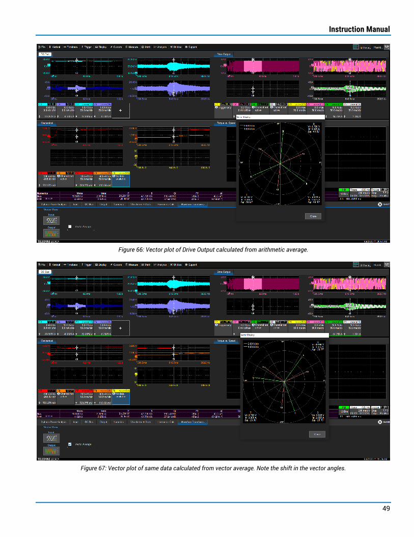
Instruction Manual
49
Figure 66: Vector plot of Drive Output calculated from arithmetic average.
Figure 67: Vector plot of same data calculated from vector average. Note the shift in the vector angles.

3-phase Power Analysis Software
50
Vector Calculation Method You may choose to calculate and display the vectors according to an arithmetic average (as done in the Numerics table) or a vector average. In both cases, the display of the first vector in the sequence is arbitrary with respect to zero degrees, and the other vector phase angles are calculated with reference to the first vector angle.
Arithmetic Average By default (with the Vector Average checkbox deselected), the vector magnitude and phase values in the vector display are calculated on the arithmetic average of the line voltage input and/or output values and line currents. Therefore, this data will exactly match the Numerics table data. However, if the selected Wiring Configuration requires line-line voltage probing, and a L-L to L-N conversion has not been performed, it will be performed automatically prior to first display of the vector. Refer to the appendix tables for details on these calculations.
Vector Average Selecting the Vector Average checkbox will cause the plots to be calculated according to the vector average. In this case, the calculated RMS voltages and currents and phase angles are described in polar notation.
To compute the vector average, the software converts polar to cartesian notation, then takes the arithmetic average of the cartesian values. It then converts these arithmetic averages back to polar notation to plot the magnitude of the RMS voltage and current vectors, and the angle between the voltage and current vectors.

Instruction Manual
51
Waveform Transformations Option Processing 3-phase waveforms is a computationally intensive task, given constantly varying voltages and currents. The Waveform Transformations option adds the ability to calculate and display αβɣ (Clarke) and dq0 (Park) transformations on Input and Output waveforms for more efficient processing.
A Line-Line to Line-Neutral (L-L to L-N) conversion is required to apply transformations.
Transformation Types The αβɣ (Clarke) transform takes 3-phase voltages/currents and transforms them to a new domain, thereby allowing representation in a 2-D plane.
The dq0 (Park) transform takes Clarke waveforms and transforms them into fixed values.
Applying Transformations 1. Open the Input or Output waveform dialog and select L-L to L-N conversion.
NOTE: The Transform Type field will remain disabled (gray) until you enable L-L to L-N conversion.
2. From Transform Method, choose (αβɣ) or (dq0).
Voltage waveforms are relabeled Vα/Vβ/Vɣ or Vd/Vq/V0, and current waveforms likewise are relabeled Iα/Iβ/Iɣ or Id/Iq/I0 on the Numerics table, descriptor boxes and dialogs.
3. Open the Waveform Transforms dialog (see bottom p.88) and select the Converted Waveforms to display.
4. Optionally, use the Converted Waveform Zoom controls to adjust center and/or vertical scale.
5. On the Numerics dialog, select the Transform(s) to add to the Numerics table:
• First, choose the Input (ABC xxx) or Output (RST xxx) transforms to add. Only the transforms that are enabled on the Input or Output dialogs will be available for selection.
• Then, choose to add the V or I values. Both V and I columns can be added to the table.

3-phase Power Analysis Software
52
Figure 68: Clarke transformed Output current waveform display.
Figure 69: Park transformed Output voltage and current waveform display.

Instruction Manual
53
Appendix A: Measurement Best Practices A variety of measurement “best practices” should be followed when making 3-phase voltage, current and power measurements that require the highest accuracies. If these practices are not followed, measurement accuracy will be reduced. We have provided enough background description of each “best practice” that the best decision can be made about whether it is necessary to follow or not, based on the degree of measurement accuracy desired.
Highest Importance for Achieving Best Accuracy
• Allow for recommended warm-up times (p.53)
• Auto Zero differential probes (p.54)
• Degauss current probes (p.54)
• Deskew non-Teledyne LeCroy current or voltage measurement devices (p.55)
• Choose the correct Sync signal for measurements (p.55)
Medium Importance for Achieving Best Accuracy
• Avoid use of non-zero offset values (p.56)
• Maximize use of vertical grid (p.56)
Lowest Importance for Achieving Best Accuracy
• Compensate passive probes (p.56)
• Apply filters to lower noise (p.57)
• Deskew Teledyne LeCroy voltage and current probes (p.57)
In addition to the instructions below, see your oscilloscope Operator’s Manual or the pertinent probe manual for more information about performing each practice.
Allow for Recommended Warm-up Times To ensure accurate measurements, allow active probes to warm-up for the recommended amount of time before autozeroing, degaussing or performing critical measurements. 20 minutes is the recommended warm-up time for most Teledyne LeCroy instruments and probes.
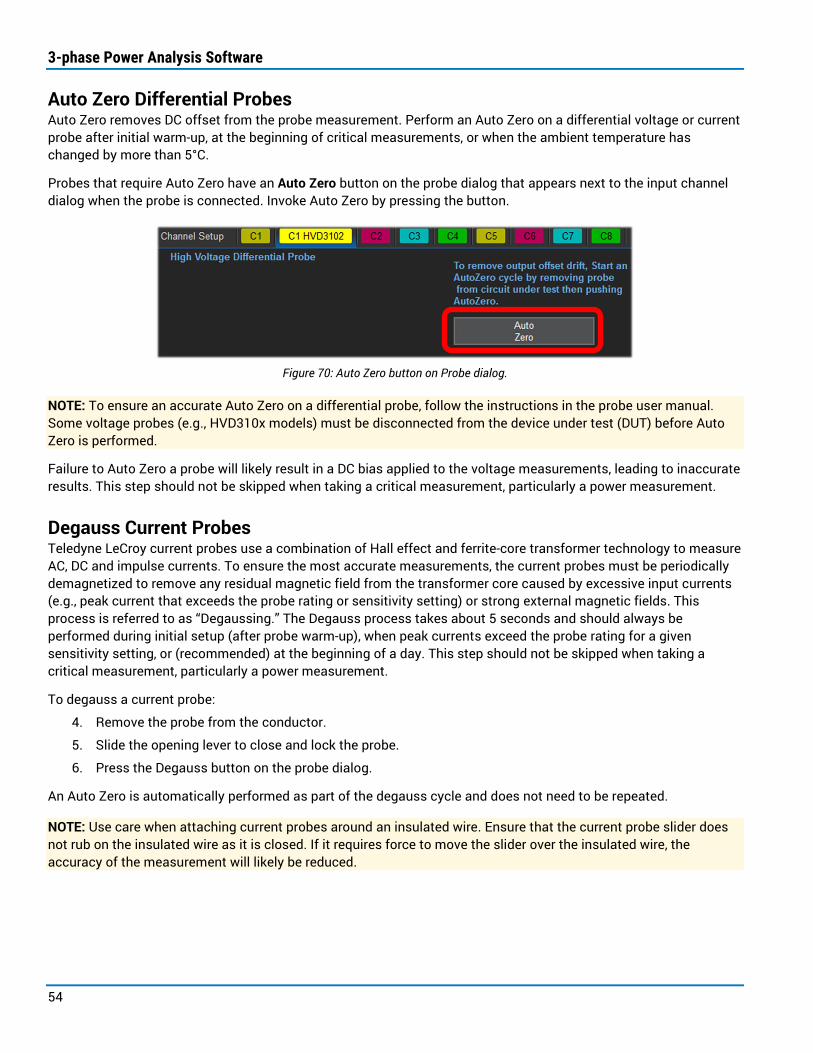
3-phase Power Analysis Software
54
Auto Zero Differential Probes Auto Zero removes DC offset from the probe measurement. Perform an Auto Zero on a differential voltage or current probe after initial warm-up, at the beginning of critical measurements, or when the ambient temperature has changed by more than 5°C.
Probes that require Auto Zero have an Auto Zero button on the probe dialog that appears next to the input channel dialog when the probe is connected. Invoke Auto Zero by pressing the button.
Figure 70: Auto Zero button on Probe dialog.
NOTE: To ensure an accurate Auto Zero on a differential probe, follow the instructions in the probe user manual. Some voltage probes (e.g., HVD310x models) must be disconnected from the device under test (DUT) before Auto Zero is performed.
Failure to Auto Zero a probe will likely result in a DC bias applied to the voltage measurements, leading to inaccurate results. This step should not be skipped when taking a critical measurement, particularly a power measurement.
Degauss Current Probes Teledyne LeCroy current probes use a combination of Hall effect and ferrite-core transformer technology to measure AC, DC and impulse currents. To ensure the most accurate measurements, the current probes must be periodically demagnetized to remove any residual magnetic field from the transformer core caused by excessive input currents (e.g., peak current that exceeds the probe rating or sensitivity setting) or strong external magnetic fields. This process is referred to as “Degaussing.” The Degauss process takes about 5 seconds and should always be performed during initial setup (after probe warm-up), when peak currents exceed the probe rating for a given sensitivity setting, or (recommended) at the beginning of a day. This step should not be skipped when taking a critical measurement, particularly a power measurement.
To degauss a current probe:
4. Remove the probe from the conductor.
5. Slide the opening lever to close and lock the probe.
6. Press the Degauss button on the probe dialog.
An Auto Zero is automatically performed as part of the degauss cycle and does not need to be repeated.
NOTE: Use care when attaching current probes around an insulated wire. Ensure that the current probe slider does not rub on the insulated wire as it is closed. If it requires force to move the slider over the insulated wire, the accuracy of the measurement will likely be reduced.

Instruction Manual
55
Deskew non-Teledyne LeCroy Current or Voltage Measurement Devices Cables, probes and other measurement devices introduce a propagation delay from the measurement point back to the input channel of the oscilloscope. In general, Teledyne LeCroy voltage and current probes introduce propagation delays in the range of 1 to 15 ns. Other measurement devices may introduce more (or less) propagation delay. RG58 coaxial cable has a propagation delay of ~3 to 5ns/m (depending on construction). For precision timing measurements or best accuracy when two signals are used in a math operation (e.g., a multiplication to achieve a power value), correction for the propagation delays may be necessary depending on the signal speed(s) and necessary precision required.
“Deskew” is the process by which various propagation delays are corrected for at the input plane of the oscilloscope. To perform a deskew:
1. Measure voltage and current signals coincidently using the same signal source.
2. Enter the deskew adjustment (plus or minus) on the input channel dialog.
Figure 71: Deskew entry field on channel setup (Cn) dialog.
Teledyne LeCroy’s DCS015 Deskew Calibration Source connects to the AUX IN connector of compatible oscilloscopes and produces a set of signals that allow voltage and current probe deskew (within limitations of the current loop size). You could also use a similar device of your own construction.
The propagation delays of non-Teledyne LeCroy measurement devices should be understood so that a sensible decision can be made as to whether the propagation delays should be adjusted for (deskewed). Input (line frequency) or Output PWM periods typically have frequencies in the range of 1 to 300 Hz, and the propagation delay errors between different voltage and current measurement devices may be so small compared to the speed of the signal being measured that rigorous deskew of signals is unlikely to result in improved power measurement accuracy. For instance, a 10 ns error between a voltage and a current signal that is contained within a 10 ms (100 Hz) period would result in a miniscule measurement error – the propagation delay is 0.0001% of the measurement period. Therefore, most users do not bother to deskew probes for power measurements unless the propagation delays are much larger than what is described above.
Choose the Best Sync Signal for Measurements Sync signal selection is critical to the correct operation of the 3-phase Power Analysis software, as it determines the interval at which measurements are performed. Any measured signal that corresponds to one repetitive time period can be used as the Sync (Synchronization) signal. A signal that varies around a zero crossing (e.g., line-line probed voltage signals, or line-neutral current signals) and that experiences little change in amplitude during the complete acquisition is the best choice to Sync with. In general, this would be the signal that most closely represents a sine wave, although it is not absolutely necessary to use a sine wave.
See Sync Signal (p.15) for details and recommendations on choosing the best source.
In the case of highly distorted waveforms (e.g., six-step commutated voltage or current waveforms), you will likely find that some adjustment of the Low Pass Filter (LPF) cutoff and Hysteresis (zero-crossing filter) settings is
3-phase Power Analysis Software
56
necessary. You can view the low-pass-filtered Sync signal, and in doing so, gain a better understanding of whether the software has a good periodic signal to determine zero-crossing times.
Signals with very high harmonic content (e.g., six-step commutated voltage signals) will have significant attenuation when the low pass filter is applied and may therefore be less suitable as a Sync signal. Signals that experience wide dynamic ranges, such as load current signals in acquisitions under highly dynamic loading conditions, may also be unsuitable. Thus, the choice of the Sync signal requires some thought prior to set up, and perhaps a visual inspection of the filtered Sync signal, to achieve accurate power measurement results.
If in doubt as to the suitability of the chosen Sync signal, or the correctness of the settings to determine the correct zero-crossings (and therefore measurement intervals), turn on the Sync signal trace and use the Zoom+Gate controls to visually determine whether correct period determination is being made.
Avoid Non-Zero Offset Values If possible, avoid adding channel offset when taking critical voltage, current or power measurements. By adding offset to the channel, offset error is introduced. When probing voltage signals line-reference, use of offset likely cannot be avoided. However, when probing voltage signals line-line, the peak positive voltage will be equal to the peak negative voltage, and offset can be set to zero while still maximizing the signal on the vertical grid. Best practice is to ensure that offset is set to zero, in this case, before making critical measurements.
Maximize Use of Vertical Grid Each display grid is divided into 8 vertical divisions and 10 horizontal divisions. The 12-bit ADC resolution (4096 discrete levels) is divided equally amongst the 8 vertical divisions, with the front-end gain range (eight times the V/div setting) determining the peak-to-peak voltage represented by full scale (8 vertical divisions).
You will obtain the best accuracy for any voltage, current or power measurement by maximizing the size of the signal on the vertical grid, therefore utilizing the maximum amount of ADC counts to resolve the displayed signal. This is different than with many power analyzers that reserve a portion of the vertical grid for overshoot (based on a user-defined or factory-default crest factor assumption). Be sure to reserve an appropriate amount of the vertical grid for expected signal overshoots or dynamic range.
NOTE: Pre-processing bandwidth filters (such as ERes) are applied by the software after the hardware acquisition but before the signal is displayed. Therefore, it is recommended to first observe signals on the display grid without ERes applied so as to set the appropriate V/div (gain) for each channel. Then, apply ERes as necessary to filter the bandwidth further.
Utilize multi-grid or Q-Scape displays—or both—to view many signals when they are maximized on the vertical axis and connect to a high-resolution external monitor to enlarge the display view. To view signal details, create a zoom of the original trace and expand the zoom trace vertically instead of changing the channel V/div.
Compensate Passive Probes The passive probes supplied with the oscilloscope are matched to the input impedance of the instrument but will need capacitive compensation (“trimming”) to accurately match the probe input impedance and achieve the best frequency response and step response signal fidelity. Perform a low-frequency calibration using the Cal signal available from the oscilloscope’s front panel. Follow the directions in the probe instruction manual to compensate the frequency response of the probes.
NOTE: On 8-channel oscilloscopes, the top row of analog inputs (C1 through C4) may have small differences in input impedance (~1 pF input capacitance difference) from the bottom row of analog inputs (C5 through C8). For best accuracy, perform a new low-frequency calibration if the probe is moved from a top-row to a bottom-row channel.
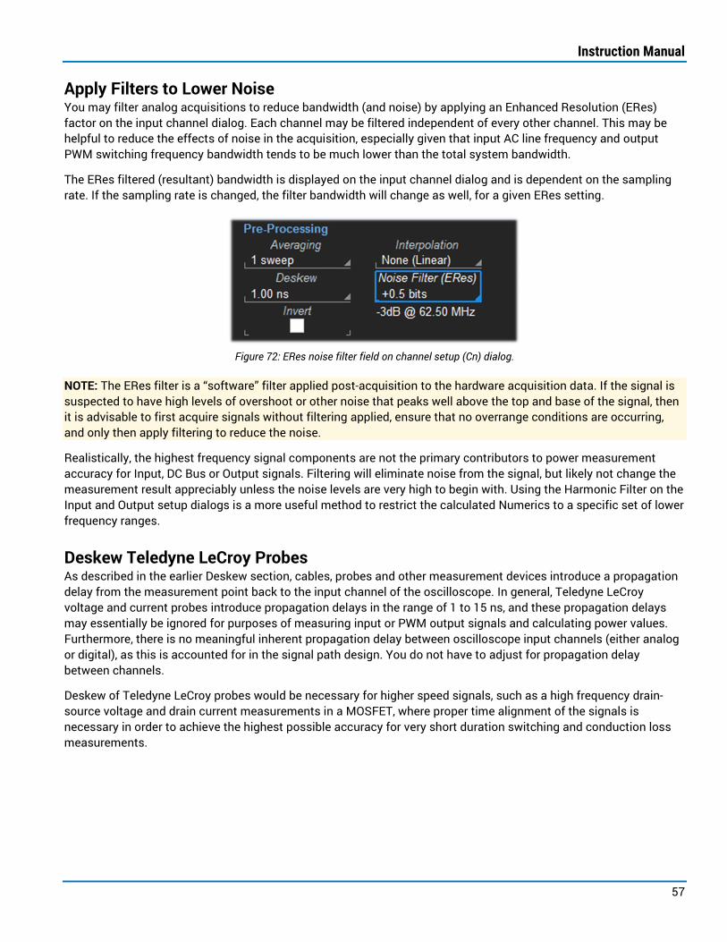
Instruction Manual
57
Apply Filters to Lower Noise You may filter analog acquisitions to reduce bandwidth (and noise) by applying an Enhanced Resolution (ERes) factor on the input channel dialog. Each channel may be filtered independent of every other channel. This may be helpful to reduce the effects of noise in the acquisition, especially given that input AC line frequency and output PWM switching frequency bandwidth tends to be much lower than the total system bandwidth.
The ERes filtered (resultant) bandwidth is displayed on the input channel dialog and is dependent on the sampling rate. If the sampling rate is changed, the filter bandwidth will change as well, for a given ERes setting.
Figure 72: ERes noise filter field on channel setup (Cn) dialog.
NOTE: The ERes filter is a “software” filter applied post-acquisition to the hardware acquisition data. If the signal is suspected to have high levels of overshoot or other noise that peaks well above the top and base of the signal, then it is advisable to first acquire signals without filtering applied, ensure that no overrange conditions are occurring, and only then apply filtering to reduce the noise.
Realistically, the highest frequency signal components are not the primary contributors to power measurement accuracy for Input, DC Bus or Output signals. Filtering will eliminate noise from the signal, but likely not change the measurement result appreciably unless the noise levels are very high to begin with. Using the Harmonic Filter on the Input and Output setup dialogs is a more useful method to restrict the calculated Numerics to a specific set of lower frequency ranges.
Deskew Teledyne LeCroy Probes As described in the earlier Deskew section, cables, probes and other measurement devices introduce a propagation delay from the measurement point back to the input channel of the oscilloscope. In general, Teledyne LeCroy voltage and current probes introduce propagation delays in the range of 1 to 15 ns, and these propagation delays may essentially be ignored for purposes of measuring input or PWM output signals and calculating power values. Furthermore, there is no meaningful inherent propagation delay between oscilloscope input channels (either analog or digital), as this is accounted for in the signal path design. You do not have to adjust for propagation delay between channels.
Deskew of Teledyne LeCroy probes would be necessary for higher speed signals, such as a high frequency drain-source voltage and drain current measurements in a MOSFET, where proper time alignment of the signals is necessary in order to achieve the highest possible accuracy for very short duration switching and conduction loss measurements.

3-phase Power Analysis Software
58
Appendix B: Calculation Methods and Formulas
Impact of Wiring Configuration on Calculations Each section of the power conversion system has one or more wiring configurations defined. The wiring configuration defines the user connection and setup of voltage and current probes, and the calculation methodology for the per-cycle measurement and Numerics table values.
Three Wattmeter Measurements For 3-phase, 4-wire (3V3A) and 3-phase, 3-wire (3V3A) wiring configurations, calculations are made using a three wattmeter method. In this case, line-neutral or line-reference voltages and line currents for each phase are available, and power (P, S, Q, λ, and ϕ) measurements on all three phases can be directly made with the associated voltage and current waveforms using a wattmeter for each phase.
With highly distorted waveforms, such as pulse-width modulated inverter waveforms, the common-mode line-reference output voltage will be significantly greater than zero. Small DC offsets in the current measurement can have large impacts in the real power (P) measurements when the Full Spectrum is used for measurements. In this case, invoking the Harmonic Filter might be justified. Furthermore, small DC offsets will cause a high calculated value of apparent power (S), which will result in high reactive power (Q) phase angle (ϕ) calculations, and subsequently a low power factor (λ) calculation. If these values are important to know with accuracy, it is recommended to use the Harmonic Filter settings to not include DC in the calculation.
For 3-phase, 3-wire (2V2A) wiring configurations where a Line-Line to Line-Neutral conversion is performed, power calculations are also made using a three wattmeter method. This conversion assumes a balanced 3-phase system for voltage and current to solve for one of the 3-phase line currents (IC or IT) using the assumption that the sum of all 3-phase line currents is zero, and using the assumption that the sum of all 3-phase line-line voltages is zero. If the system is not balanced (e.g., due to leakage currents to ground), then the assumption is incorrect and results will differ from that of a three wattmeter method.
Two Wattmeter Measurements For 3-phase, 3-wire (2V2A) wiring configurations that are probed Line-Line (no conversion), calculations are made using a two wattmeter method. In this case, line-line voltages are available along with line currents, but they do not associate directly with a line current, so while two power values are provided, the two power levels will not be balanced. They will, however, add up to the correct 3-phase power.
The two wattmeter method assumes a balanced 3-phase system. In this case, the IC or IT current in the 3-phase system is ignored.
For 1-phase, 3-wire (2V2A) wiring configurations, power calculations are also made using a two wattmeter measurement. By definition, these voltages are measured line-neutral, so there are two pairs of directly associated line voltages and currents. These two power values will add to the total single-phase power.
One Wattmeter Measurements 1-phase, 2-wire (1V1A) wiring configuration power calculations are made using a one wattmeter measurement. By definition, the voltage is line-neutral, and there is only one pair of directly associated line voltage and currents.
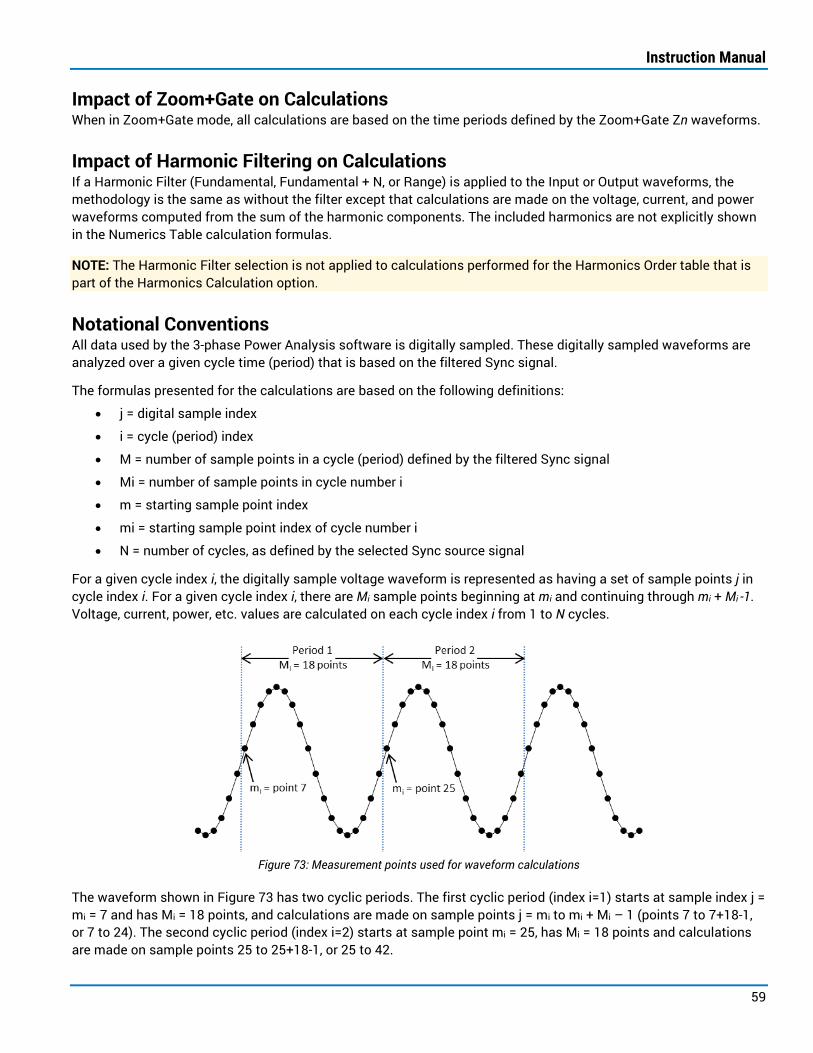
Instruction Manual
59
Impact of Zoom+Gate on Calculations When in Zoom+Gate mode, all calculations are based on the time periods defined by the Zoom+Gate Zn waveforms.
Impact of Harmonic Filtering on Calculations If a Harmonic Filter (Fundamental, Fundamental + N, or Range) is applied to the Input or Output waveforms, the methodology is the same as without the filter except that calculations are made on the voltage, current, and power waveforms computed from the sum of the harmonic components. The included harmonics are not explicitly shown in the Numerics Table calculation formulas.
NOTE: The Harmonic Filter selection is not applied to calculations performed for the Harmonics Order table that is part of the Harmonics Calculation option.
Notational Conventions All data used by the 3-phase Power Analysis software is digitally sampled. These digitally sampled waveforms are analyzed over a given cycle time (period) that is based on the filtered Sync signal.
The formulas presented for the calculations are based on the following definitions:
• j = digital sample index
• i = cycle (period) index
• M = number of sample points in a cycle (period) defined by the filtered Sync signal
• Mi = number of sample points in cycle number i
• m = starting sample point index
• mi = starting sample point index of cycle number i
• N = number of cycles, as defined by the selected Sync source signal
For a given cycle index i, the digitally sample voltage waveform is represented as having a set of sample points j in cycle index i. For a given cycle index i, there are Mi sample points beginning at mi and continuing through mi + Mi -1. Voltage, current, power, etc. values are calculated on each cycle index i from 1 to N cycles.
Figure 73: Measurement points used for waveform calculations
The waveform shown in Figure 73 has two cyclic periods. The first cyclic period (index i=1) starts at sample index j = mi = 7 and has Mi = 18 points, and calculations are made on sample points j = mi to mi + Mi – 1 (points 7 to 7+18-1, or 7 to 24). The second cyclic period (index i=2) starts at sample point mi = 25, has Mi = 18 points and calculations are made on sample points 25 to 25+18-1, or 25 to 42.
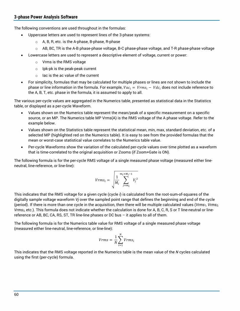
3-phase Power Analysis Software
60
The following conventions are used throughout in the formulas:
• Uppercase letters are used to represent lines of the 3-phase systems:
o A, B, R, etc. is the A-phase, B-phase, R-phase
o AB, BC, TR is the A-B phase-phase voltage, B-C phase-phase voltage, and T-R phase-phase voltage
• Lowercase letters are used to represent a descriptive element of voltage, current or power:
o Vrms is the RMS voltage
o Ipk-pk is the peak-peak current
o Iac is the ac value of the current
• For simplicity, formulas that may be calculated for multiple phases or lines are not shown to include the phase or line information in the formula. For example, 𝑉𝑉𝐸𝐸𝐸𝐸𝑖𝑖 = 𝑉𝑉𝑎𝑎𝑎𝑎𝑉𝑉𝑖𝑖 − 𝑉𝑉𝑜𝑜𝐸𝐸𝑖𝑖 does not include reference to the A, B, T, etc. phase in the formula, it is assumed to apply to all.
The various per-cycle values are aggregated in the Numerics table, presented as statistical data in the Statistics table, or displayed as a per-cycle Waveform.
• Values shown on the Numerics table represent the mean/peak of a specific measurement on a specific source, or an MP. The Numerics table MP Vrms(A) is the RMS voltage of the A phase voltage. Refer to the example below.
• Values shown on the Statistics table represent the statistical mean, min, max, standard deviation, etc. of a selected MP (highlighted red on the Numerics table). It is easy to see from the provided formulas that the mean or worst-case statistical value correlates to the Numerics table value.
• Per-cycle Waveforms show the variation of the calculated per-cycle values over time plotted as a waveform that is time-correlated to the original acquisition or Zooms (if Zoom+Gate is ON).
The following formula is for the per-cycle RMS voltage of a single measured phase voltage (measured either line-neutral, line-reference, or line-line):
𝑉𝑉𝑎𝑎𝑎𝑎𝑉𝑉𝑖𝑖 = �1𝑀𝑀𝑖𝑖
� 𝑉𝑉𝑗𝑗2𝑚𝑚𝑖𝑖+𝑀𝑀𝑖𝑖−1
𝑗𝑗=𝑚𝑚𝑖𝑖
This indicates that the RMS voltage for a given cycle (cycle i) is calculated from the root-sum-of-squares of the digitally sample voltage waveform Vj over the sampled point range that defines the beginning and end of the cycle (period). If there is more than one cycle in the acquisition, then there will be multiple calculated values (Vrms1, Vrms2, Vrms3, etc.). This formula does not indicate whether the calculation is done for A, B, C, R, S or T line-neutral or line-reference or AB, BC, CA, RS, ST, TR line-line phases or DC bus – it applies to all of them.
The following formula is for the Numerics table value for RMS voltage of a single measured phase voltage (measured either line-neutral, line-reference, or line-line):
𝑉𝑉𝑎𝑎𝑎𝑎𝑉𝑉 = 1𝑁𝑁�𝑉𝑉𝑎𝑎𝑎𝑎𝑉𝑉𝑖𝑖
𝑁𝑁
𝑖𝑖=1
This indicates that the RMS voltage reported in the Numerics table is the mean value of the N cycles calculated using the first (per-cycle) formula.

Instruction Manual
61
3-phase 4-wire (3V3A) Calculations In this case, a Neutral is present, voltage is probed Line-Neutral and Line currents are sensed. The calculation methodology for Voltage, Current and Power is summarized in the tables below. The line-neutral voltage values and line current values are shown as A, B, C, R, S, and T.
VRMS (Line-Neutral) IRMS (Line-Neutral)
A, B, C, R, S, T
𝑉𝑉𝑎𝑎𝑎𝑎𝑉𝑉𝑖𝑖 = �1𝑀𝑀𝑖𝑖
� 𝑉𝑉𝑗𝑗2𝑚𝑚𝑖𝑖+𝑀𝑀𝑖𝑖−1
𝑗𝑗=𝑚𝑚𝑖𝑖
𝑉𝑉𝑎𝑎𝑎𝑎𝑉𝑉 = 1𝑁𝑁�𝑉𝑉𝑎𝑎𝑎𝑎𝑉𝑉𝑖𝑖
𝑁𝑁
𝑖𝑖=1
𝐼𝐼𝑎𝑎𝑎𝑎𝑉𝑉𝑖𝑖 = �1𝑀𝑀𝑖𝑖
� 𝐼𝐼𝑗𝑗2𝑚𝑚𝑖𝑖+𝑀𝑀𝑖𝑖−1
𝑗𝑗=𝑚𝑚𝑖𝑖
𝐼𝐼𝑎𝑎𝑎𝑎𝑉𝑉 = 1𝑁𝑁�𝐼𝐼𝑎𝑎𝑎𝑎𝑉𝑉𝑖𝑖
𝑁𝑁
𝑖𝑖=1
ΣABC
𝑉𝑉𝑎𝑎𝑎𝑎𝑉𝑉𝛴𝛴𝛴𝛴𝛴𝛴𝛴𝛴𝑖𝑖 = 13
(𝑉𝑉𝑎𝑎𝑎𝑎𝑉𝑉𝛴𝛴𝑖𝑖 + 𝑉𝑉𝑎𝑎𝑎𝑎𝑉𝑉𝛴𝛴𝑖𝑖 + 𝑉𝑉𝑎𝑎𝑎𝑎𝑉𝑉𝛴𝛴𝑖𝑖)
𝑉𝑉𝑎𝑎𝑎𝑎𝑉𝑉𝛴𝛴𝛴𝛴𝛴𝛴𝛴𝛴 = 1𝑁𝑁�𝑉𝑉𝑎𝑎𝑎𝑎𝑉𝑉𝛴𝛴𝛴𝛴𝛴𝛴𝛴𝛴𝑖𝑖
𝑁𝑁
𝑖𝑖=1
𝐼𝐼𝑎𝑎𝑎𝑎𝑉𝑉𝛴𝛴𝛴𝛴𝛴𝛴𝛴𝛴𝑖𝑖 = 13
(𝐼𝐼𝑎𝑎𝑎𝑎𝑉𝑉𝛴𝛴𝑖𝑖 + 𝐼𝐼𝑎𝑎𝑎𝑎𝑉𝑉𝛴𝛴𝑖𝑖 + 𝐼𝐼𝑎𝑎𝑎𝑎𝑉𝑉𝛴𝛴𝑖𝑖)
𝐼𝐼𝑎𝑎𝑎𝑎𝑉𝑉𝛴𝛴𝛴𝛴𝛴𝛴𝛴𝛴 = 1𝑁𝑁�𝐼𝐼𝑎𝑎𝑎𝑎𝑉𝑉𝛴𝛴𝛴𝛴𝛴𝛴𝛴𝛴𝑖𝑖
𝑁𝑁
𝑖𝑖=1
ΣRST
𝑉𝑉𝑎𝑎𝑎𝑎𝑉𝑉𝛴𝛴𝛴𝛴𝛴𝛴𝛴𝛴𝑖𝑖 = 13
(𝑉𝑉𝑎𝑎𝑎𝑎𝑉𝑉𝛴𝛴𝑖𝑖 + 𝑉𝑉𝑎𝑎𝑎𝑎𝑉𝑉𝛴𝛴𝑖𝑖 + 𝑉𝑉𝑎𝑎𝑎𝑎𝑉𝑉𝛴𝛴𝑖𝑖)
𝑉𝑉𝑎𝑎𝑎𝑎𝑉𝑉𝛴𝛴𝛴𝛴𝛴𝛴𝛴𝛴 = 1𝑁𝑁�𝑉𝑉𝑎𝑎𝑎𝑎𝑉𝑉𝛴𝛴𝛴𝛴𝛴𝛴𝛴𝛴𝑖𝑖
𝑁𝑁
𝑖𝑖=1
𝐼𝐼𝑎𝑎𝑎𝑎𝑉𝑉𝛴𝛴𝛴𝛴𝛴𝛴𝛴𝛴𝑖𝑖 = 13
(𝐼𝐼𝑎𝑎𝑎𝑎𝑉𝑉𝛴𝛴𝑖𝑖 + 𝐼𝐼𝑎𝑎𝑎𝑎𝑉𝑉𝛴𝛴𝑖𝑖 + 𝐼𝐼𝑎𝑎𝑎𝑎𝑉𝑉𝛴𝛴𝑖𝑖)
𝐼𝐼𝑎𝑎𝑎𝑎𝑉𝑉𝛴𝛴𝛴𝛴𝛴𝛴𝛴𝛴 = 1𝑁𝑁�𝐼𝐼𝑎𝑎𝑎𝑎𝑉𝑉𝛴𝛴𝛴𝛴𝛴𝛴𝛴𝛴𝑖𝑖
𝑁𝑁
𝑖𝑖=1
VDC (Line-Neutral) IDC (Line-Neutral)
A, B, C, R, S, T
𝑉𝑉𝑜𝑜𝐸𝐸𝑖𝑖 = 1𝑀𝑀𝑖𝑖
� 𝑉𝑉𝑗𝑗
𝑚𝑚𝑖𝑖+𝑀𝑀𝑖𝑖−1
𝑗𝑗=𝑚𝑚𝑖𝑖
𝑉𝑉𝑜𝑜𝐸𝐸 = 1𝑁𝑁�𝑉𝑉𝑜𝑜𝐸𝐸𝑖𝑖
𝑁𝑁
𝑖𝑖=1
𝐼𝐼𝑜𝑜𝐸𝐸𝑖𝑖 = 1𝑀𝑀𝑖𝑖
� 𝐼𝐼𝑗𝑗
𝑚𝑚𝑖𝑖+𝑀𝑀𝑖𝑖−1
𝑗𝑗=𝑚𝑚𝑖𝑖
𝐼𝐼𝑜𝑜𝐸𝐸 = 1𝑁𝑁�𝐼𝐼𝑜𝑜𝐸𝐸𝑖𝑖
𝑁𝑁
𝑖𝑖=1
ΣABC
𝑉𝑉𝑜𝑜𝐸𝐸𝛴𝛴𝛴𝛴𝛴𝛴𝛴𝛴𝑖𝑖 = 13
(𝑉𝑉𝑜𝑜𝐸𝐸𝛴𝛴𝑖𝑖 + 𝑉𝑉𝑜𝑜𝐸𝐸𝛴𝛴𝑖𝑖 + 𝑉𝑉𝑜𝑜𝐸𝐸𝛴𝛴𝑖𝑖)
𝑉𝑉𝑜𝑜𝐸𝐸𝛴𝛴𝛴𝛴𝛴𝛴𝛴𝛴 = 1𝑁𝑁�𝑉𝑉𝑜𝑜𝐸𝐸𝛴𝛴𝛴𝛴𝛴𝛴𝛴𝛴𝑖𝑖
𝑁𝑁
𝑖𝑖=1
𝐼𝐼𝑜𝑜𝐸𝐸𝛴𝛴𝛴𝛴𝛴𝛴𝛴𝛴𝑖𝑖 = 13
(𝐼𝐼𝑜𝑜𝐸𝐸𝛴𝛴𝑖𝑖 + 𝐼𝐼𝑜𝑜𝐸𝐸𝛴𝛴𝑖𝑖 + 𝐼𝐼𝑜𝑜𝐸𝐸𝛴𝛴𝑖𝑖)
𝐼𝐼𝑜𝑜𝐸𝐸𝛴𝛴𝛴𝛴𝛴𝛴𝛴𝛴 = 1𝑁𝑁�𝐼𝐼𝑜𝑜𝐸𝐸𝛴𝛴𝛴𝛴𝛴𝛴𝛴𝛴𝑖𝑖
𝑁𝑁
𝑖𝑖=1
ΣRST
𝑉𝑉𝑜𝑜𝐸𝐸𝛴𝛴𝛴𝛴𝛴𝛴𝛴𝛴𝑖𝑖 = 13
(𝑉𝑉𝑜𝑜𝐸𝐸𝛴𝛴𝑖𝑖 + 𝑉𝑉𝑜𝑜𝐸𝐸𝛴𝛴𝑖𝑖 + 𝑉𝑉𝑜𝑜𝐸𝐸𝛴𝛴𝑖𝑖)
𝑉𝑉𝑜𝑜𝐸𝐸𝛴𝛴𝛴𝛴𝛴𝛴𝛴𝛴 = 1𝑁𝑁�𝑉𝑉𝑜𝑜𝐸𝐸𝛴𝛴𝛴𝛴𝛴𝛴𝛴𝛴𝑖𝑖
𝑁𝑁
𝑖𝑖=1
𝐼𝐼𝑜𝑜𝐸𝐸𝛴𝛴𝛴𝛴𝛴𝛴𝛴𝛴𝑖𝑖 = 13
(𝐼𝐼𝑜𝑜𝐸𝐸𝛴𝛴𝑖𝑖 + 𝐼𝐼𝑜𝑜𝐸𝐸𝛴𝛴𝑖𝑖 + 𝐼𝐼𝑜𝑜𝐸𝐸𝛴𝛴𝑖𝑖)
𝐼𝐼𝑜𝑜𝐸𝐸𝛴𝛴𝛴𝛴𝛴𝛴𝛴𝛴 = 1𝑁𝑁�𝐼𝐼𝑜𝑜𝐸𝐸𝛴𝛴𝛴𝛴𝛴𝛴𝛴𝛴𝑖𝑖
𝑁𝑁
𝑖𝑖=1

3-phase Power Analysis Software
62
VAC (Line-Neutral) IAC (Line-Neutral)
A, B, C, R, S, T
𝑉𝑉𝐸𝐸𝐸𝐸𝑖𝑖 = 𝑉𝑉𝑎𝑎𝑎𝑎𝑉𝑉𝑖𝑖 − 𝑉𝑉𝑜𝑜𝐸𝐸𝑖𝑖
𝑉𝑉𝐸𝐸𝐸𝐸 = 1𝑁𝑁�𝑉𝑉𝐸𝐸𝐸𝐸𝑖𝑖
𝑁𝑁
𝑖𝑖=1
𝐼𝐼𝐸𝐸𝐸𝐸𝑖𝑖 = 𝐼𝐼𝑎𝑎𝑎𝑎𝑉𝑉𝑖𝑖 − 𝐼𝐼𝑜𝑜𝐸𝐸𝑖𝑖
𝐼𝐼𝐸𝐸𝐸𝐸 = 1𝑁𝑁�𝐼𝐼𝐸𝐸𝐸𝐸𝑖𝑖
𝑁𝑁
𝑖𝑖=1
ΣABC
𝑉𝑉𝐸𝐸𝐸𝐸𝛴𝛴𝛴𝛴𝛴𝛴𝛴𝛴𝑖𝑖 = 13
(𝑉𝑉𝐸𝐸𝐸𝐸𝛴𝛴𝑖𝑖 + 𝑉𝑉𝐸𝐸𝐸𝐸𝛴𝛴𝑖𝑖 + 𝑉𝑉𝐸𝐸𝐸𝐸𝛴𝛴𝑖𝑖)
𝑉𝑉𝐸𝐸𝐸𝐸𝛴𝛴𝛴𝛴𝛴𝛴𝛴𝛴 = 1𝑁𝑁�𝑉𝑉𝐸𝐸𝐸𝐸𝛴𝛴𝛴𝛴𝛴𝛴𝛴𝛴𝑖𝑖
𝑁𝑁
𝑖𝑖=1
𝐼𝐼𝐸𝐸𝐸𝐸𝛴𝛴𝛴𝛴𝛴𝛴𝛴𝛴𝑖𝑖 = 13
(𝐼𝐼𝐸𝐸𝐸𝐸𝛴𝛴𝑖𝑖 + 𝐼𝐼𝐸𝐸𝐸𝐸𝛴𝛴𝑖𝑖 + 𝐼𝐼𝐸𝐸𝐸𝐸𝛴𝛴𝑖𝑖)
𝐼𝐼𝐸𝐸𝐸𝐸𝛴𝛴𝛴𝛴𝛴𝛴𝛴𝛴 = 1𝑁𝑁�𝐼𝐼𝐸𝐸𝐸𝐸𝛴𝛴𝛴𝛴𝛴𝛴𝛴𝛴𝑖𝑖
𝑁𝑁
𝑖𝑖=1
ΣRST
𝑉𝑉𝐸𝐸𝐸𝐸𝛴𝛴𝛴𝛴𝛴𝛴𝛴𝛴𝑖𝑖 = 13
(𝑉𝑉𝐸𝐸𝐸𝐸𝛴𝛴𝑖𝑖 + 𝑉𝑉𝐸𝐸𝐸𝐸𝛴𝛴𝑖𝑖 + 𝑉𝑉𝐸𝐸𝐸𝐸𝛴𝛴𝑖𝑖)
𝑉𝑉𝐸𝐸𝐸𝐸𝛴𝛴𝛴𝛴𝛴𝛴𝛴𝛴 = 1𝑁𝑁�𝑉𝑉𝐸𝐸𝐸𝐸𝛴𝛴𝛴𝛴𝛴𝛴𝛴𝛴𝑖𝑖
𝑁𝑁
𝑖𝑖=1
𝐼𝐼𝐸𝐸𝐸𝐸𝛴𝛴𝛴𝛴𝛴𝛴𝛴𝛴𝑖𝑖 = 13
(𝐼𝐼𝐸𝐸𝐸𝐸𝛴𝛴𝑖𝑖 + 𝐼𝐼𝐸𝐸𝐸𝐸𝛴𝛴𝑖𝑖 + 𝐼𝐼𝐸𝐸𝐸𝐸𝛴𝛴𝑖𝑖)
𝐼𝐼𝐸𝐸𝐸𝐸𝛴𝛴𝛴𝛴𝛴𝛴𝛴𝛴 = 1𝑁𝑁�𝐼𝐼𝐸𝐸𝐸𝐸𝛴𝛴𝛴𝛴𝛴𝛴𝛴𝛴𝑖𝑖
𝑁𝑁
𝑖𝑖=1
VPK+, VPK-, VPK-PK (Line-Neutral) IPK+, IPK-, IPK-PK (Line-Neutral)
A, B, C, R, S, T
𝑉𝑉𝑐𝑐𝑉𝑉⁺𝑖𝑖 = max𝑗𝑗=𝑚𝑚𝑖𝑖 𝑡𝑡𝑡𝑡 𝑚𝑚𝑖𝑖+𝑀𝑀𝑖𝑖−1
𝑉𝑉𝑗𝑗
𝑉𝑉𝑐𝑐𝑉𝑉⁻𝑖𝑖 = min𝑗𝑗=𝑚𝑚𝑖𝑖 𝑡𝑡𝑡𝑡 𝑚𝑚𝑖𝑖+𝑀𝑀𝑖𝑖−1
𝑉𝑉𝑗𝑗
𝑉𝑉𝑐𝑐𝑉𝑉⎼𝑐𝑐𝑉𝑉𝑖𝑖 = 𝑉𝑉𝑐𝑐𝑉𝑉⁺𝑖𝑖 − 𝑉𝑉𝑐𝑐𝑉𝑉⁻𝑖𝑖
𝑉𝑉𝑐𝑐𝑉𝑉+ = max𝑖𝑖=1 𝑡𝑡𝑡𝑡 𝑁𝑁
𝑉𝑉𝑐𝑐𝑉𝑉⁺𝑖𝑖
𝑉𝑉𝑐𝑐𝑉𝑉⁻ = min𝑖𝑖=1 𝑡𝑡𝑡𝑡 𝑁𝑁
𝑉𝑉𝑐𝑐𝑉𝑉⁻𝑖𝑖
𝑉𝑉𝑐𝑐𝑉𝑉⎼𝑐𝑐𝑉𝑉 = max𝑖𝑖=1 𝑡𝑡𝑡𝑡 𝑁𝑁
𝑉𝑉𝑐𝑐𝑉𝑉⎼𝑐𝑐𝑉𝑉𝑖𝑖
𝐼𝐼𝑐𝑐𝑉𝑉⁺𝑖𝑖 = max𝑗𝑗=𝑚𝑚𝑖𝑖 𝑡𝑡𝑡𝑡 𝑚𝑚𝑖𝑖+𝑀𝑀𝑖𝑖−1
𝐼𝐼𝑗𝑗
𝐼𝐼𝑐𝑐𝑉𝑉⁻𝑖𝑖 = min𝑗𝑗=𝑚𝑚𝑖𝑖 𝑡𝑡𝑡𝑡 𝑚𝑚𝑖𝑖+𝑀𝑀𝑖𝑖−1
𝐼𝐼𝑗𝑗
𝐼𝐼𝑐𝑐𝑉𝑉⎼𝑐𝑐𝑉𝑉𝑖𝑖 = 𝐼𝐼𝑐𝑐𝑉𝑉⁺𝑖𝑖 − 𝐼𝐼𝑐𝑐𝑉𝑉⁻𝑖𝑖
𝐼𝐼𝑐𝑐𝑉𝑉+ = max𝑖𝑖=1 𝑡𝑡𝑡𝑡 𝑁𝑁
𝐼𝐼𝑐𝑐𝑉𝑉⁺𝑖𝑖
𝐼𝐼𝑐𝑐𝑉𝑉⁻ = min𝑖𝑖=1 𝑡𝑡𝑡𝑡 𝑁𝑁
𝐼𝐼𝑐𝑐𝑉𝑉⁻𝑖𝑖
𝐼𝐼𝑐𝑐𝑉𝑉⎼𝑐𝑐𝑉𝑉 = max𝑖𝑖=1 𝑡𝑡𝑡𝑡 𝑁𝑁
𝐼𝐼𝑐𝑐𝑉𝑉⎼𝑐𝑐𝑉𝑉𝑖𝑖
ΣABC
𝑉𝑉𝑐𝑐𝑉𝑉+𝛴𝛴𝛴𝛴𝛴𝛴𝛴𝛴𝑖𝑖 = max�𝑉𝑉𝑐𝑐𝑉𝑉+𝛴𝛴𝑖𝑖 ,𝑉𝑉𝑐𝑐𝑉𝑉+𝛴𝛴𝑖𝑖 ,𝑉𝑉𝑐𝑐𝑉𝑉
+𝛴𝛴𝑖𝑖�
𝑉𝑉𝑐𝑐𝑉𝑉⁻𝛴𝛴𝛴𝛴𝛴𝛴𝛴𝛴𝑖𝑖 = min�𝑉𝑉𝑐𝑐𝑉𝑉⁻𝛴𝛴𝑖𝑖 ,𝑉𝑉𝑐𝑐𝑉𝑉⁻𝛴𝛴𝑖𝑖 ,𝑉𝑉𝑐𝑐𝑉𝑉
⁻𝛴𝛴𝑖𝑖�
𝑉𝑉𝑐𝑐𝑉𝑉⎼𝑐𝑐𝑉𝑉𝛴𝛴𝛴𝛴𝛴𝛴𝛴𝛴𝑖𝑖 = max(𝑉𝑉𝑐𝑐𝑉𝑉⎼𝑐𝑐𝑉𝑉𝛴𝛴𝑖𝑖 ,𝑉𝑉𝑐𝑐𝑉𝑉⎼𝑐𝑐𝑉𝑉𝛴𝛴𝑖𝑖 ,𝑉𝑉𝑐𝑐𝑉𝑉⎼𝑐𝑐𝑉𝑉𝛴𝛴𝑖𝑖)
𝑉𝑉𝑐𝑐𝑉𝑉+𝛴𝛴𝛴𝛴𝛴𝛴𝛴𝛴 = max𝑖𝑖=1 𝑡𝑡𝑡𝑡 𝑁𝑁
𝑉𝑉𝑐𝑐𝑉𝑉+𝛴𝛴𝛴𝛴𝛴𝛴𝛴𝛴𝑖𝑖
𝑉𝑉𝑐𝑐𝑉𝑉⁻𝛴𝛴𝛴𝛴𝛴𝛴𝛴𝛴 = min𝑖𝑖=1 𝑡𝑡𝑡𝑡 𝑁𝑁
𝑉𝑉𝑐𝑐𝑉𝑉⁻𝛴𝛴𝛴𝛴𝛴𝛴𝛴𝛴𝑖𝑖
𝑉𝑉𝑐𝑐𝑉𝑉⎼𝑐𝑐𝑉𝑉𝛴𝛴𝛴𝛴𝛴𝛴𝛴𝛴 = max𝑖𝑖=1 𝑡𝑡𝑡𝑡 𝑁𝑁
𝑉𝑉𝑐𝑐𝑉𝑉⎼𝑐𝑐𝑉𝑉𝛴𝛴𝛴𝛴𝛴𝛴𝛴𝛴𝑖𝑖
𝐼𝐼𝑐𝑐𝑉𝑉+𝛴𝛴𝛴𝛴𝛴𝛴𝛴𝛴𝑖𝑖 = max�𝐼𝐼𝑐𝑐𝑉𝑉+𝛴𝛴𝑖𝑖 , 𝐼𝐼𝑐𝑐𝑉𝑉+𝛴𝛴𝑖𝑖 , 𝐼𝐼𝑐𝑐𝑉𝑉
+𝛴𝛴𝑖𝑖�
𝐼𝐼𝑐𝑐𝑉𝑉⁻𝛴𝛴𝛴𝛴𝛴𝛴𝛴𝛴𝑖𝑖 = min�𝐼𝐼𝑐𝑐𝑉𝑉⁻𝛴𝛴𝑖𝑖 , 𝐼𝐼𝑐𝑐𝑉𝑉⁻𝛴𝛴𝑖𝑖 , 𝐼𝐼𝑐𝑐𝑉𝑉
⁻𝛴𝛴𝑖𝑖�
𝐼𝐼𝑐𝑐𝑉𝑉⎼𝑐𝑐𝑉𝑉𝛴𝛴𝛴𝛴𝛴𝛴𝛴𝛴𝑖𝑖 = max(𝐼𝐼𝑐𝑐𝑉𝑉⎼𝑐𝑐𝑉𝑉𝛴𝛴𝑖𝑖 , 𝐼𝐼𝑐𝑐𝑉𝑉⎼𝑐𝑐𝑉𝑉𝛴𝛴𝑖𝑖 , 𝐼𝐼𝑐𝑐𝑉𝑉⎼𝑐𝑐𝑉𝑉𝛴𝛴𝑖𝑖)
𝐼𝐼𝑐𝑐𝑉𝑉+𝛴𝛴𝛴𝛴𝛴𝛴𝛴𝛴 = max𝑖𝑖=1 𝑡𝑡𝑡𝑡 𝑁𝑁
𝐼𝐼𝑐𝑐𝑉𝑉+𝛴𝛴𝛴𝛴𝛴𝛴𝛴𝛴𝑖𝑖
𝐼𝐼𝑐𝑐𝑉𝑉⁻𝛴𝛴𝛴𝛴𝛴𝛴𝛴𝛴 = min𝑖𝑖=1 𝑡𝑡𝑡𝑡 𝑁𝑁
𝐼𝐼𝑐𝑐𝑉𝑉⁻𝛴𝛴𝛴𝛴𝛴𝛴𝛴𝛴𝑖𝑖
𝐼𝐼𝑐𝑐𝑉𝑉⎼𝑐𝑐𝑉𝑉𝛴𝛴𝛴𝛴𝛴𝛴𝛴𝛴 = max𝑖𝑖=1 𝑡𝑡𝑡𝑡 𝑁𝑁
𝐼𝐼𝑐𝑐𝑉𝑉⎼𝑐𝑐𝑉𝑉𝛴𝛴𝛴𝛴𝛴𝛴𝛴𝛴𝑖𝑖
ΣRST
𝑉𝑉𝑐𝑐𝑉𝑉+𝛴𝛴𝛴𝛴𝛴𝛴𝛴𝛴𝑖𝑖 = max�𝑉𝑉𝑐𝑐𝑉𝑉+𝛴𝛴𝑖𝑖 ,𝑉𝑉𝑐𝑐𝑉𝑉+𝛴𝛴𝑖𝑖 ,𝑉𝑉𝑐𝑐𝑉𝑉
+𝛴𝛴𝑖𝑖�
𝑉𝑉𝑐𝑐𝑉𝑉⁻𝛴𝛴𝛴𝛴𝛴𝛴𝛴𝛴𝑖𝑖 = min�𝑉𝑉𝑐𝑐𝑉𝑉⁻𝛴𝛴𝑖𝑖 ,𝑉𝑉𝑐𝑐𝑉𝑉⁻𝛴𝛴𝑖𝑖 ,𝑉𝑉𝑐𝑐𝑉𝑉
⁻𝛴𝛴𝑖𝑖�
𝑉𝑉𝑐𝑐𝑉𝑉⎼𝑐𝑐𝑉𝑉𝛴𝛴𝛴𝛴𝛴𝛴𝛴𝛴𝑖𝑖 = max(𝑉𝑉𝑐𝑐𝑉𝑉⎼𝑐𝑐𝑉𝑉𝛴𝛴𝑖𝑖 ,𝑉𝑉𝑐𝑐𝑉𝑉⎼𝑐𝑐𝑉𝑉𝛴𝛴𝑖𝑖 ,𝑉𝑉𝑐𝑐𝑉𝑉⎼𝑐𝑐𝑉𝑉𝛴𝛴𝑖𝑖)
𝑉𝑉𝑐𝑐𝑉𝑉+𝛴𝛴𝛴𝛴𝛴𝛴𝛴𝛴 = max𝑖𝑖=1 𝑡𝑡𝑡𝑡 𝑁𝑁
𝑉𝑉𝑐𝑐𝑉𝑉+𝛴𝛴𝛴𝛴𝛴𝛴𝛴𝛴𝑖𝑖
𝑉𝑉𝑐𝑐𝑉𝑉⁻𝛴𝛴𝛴𝛴𝛴𝛴𝛴𝛴 = min𝑖𝑖=1 𝑡𝑡𝑡𝑡 𝑁𝑁
𝑉𝑉𝑐𝑐𝑉𝑉⁻𝛴𝛴𝛴𝛴𝛴𝛴𝛴𝛴𝑖𝑖
𝑉𝑉𝑐𝑐𝑉𝑉⎼𝑐𝑐𝑉𝑉𝛴𝛴𝛴𝛴𝛴𝛴𝛴𝛴 = max𝑖𝑖=1 𝑡𝑡𝑡𝑡 𝑁𝑁
𝑉𝑉𝑐𝑐𝑉𝑉⎼𝑐𝑐𝑉𝑉𝛴𝛴𝛴𝛴𝛴𝛴𝛴𝛴𝑖𝑖
𝐼𝐼𝑐𝑐𝑉𝑉+𝛴𝛴𝛴𝛴𝛴𝛴𝛴𝛴𝑖𝑖 = max�𝐼𝐼𝑐𝑐𝑉𝑉+𝛴𝛴𝑖𝑖 , 𝐼𝐼𝑐𝑐𝑉𝑉+𝛴𝛴𝑖𝑖 , 𝐼𝐼𝑐𝑐𝑉𝑉
+𝛴𝛴𝑖𝑖�
𝐼𝐼𝑐𝑐𝑉𝑉⁻𝛴𝛴𝛴𝛴𝛴𝛴𝛴𝛴𝑖𝑖 = min�𝐼𝐼𝑐𝑐𝑉𝑉⁻𝛴𝛴𝑖𝑖 , 𝐼𝐼𝑐𝑐𝑉𝑉⁻𝛴𝛴𝑖𝑖 , 𝐼𝐼𝑐𝑐𝑉𝑉
⁻𝛴𝛴𝑖𝑖�
𝐼𝐼𝑐𝑐𝑉𝑉⎼𝑐𝑐𝑉𝑉𝛴𝛴𝛴𝛴𝛴𝛴𝛴𝛴𝑖𝑖 = max(𝐼𝐼𝑐𝑐𝑉𝑉⎼𝑐𝑐𝑉𝑉𝛴𝛴𝑖𝑖 , 𝐼𝐼𝑐𝑐𝑉𝑉⎼𝑐𝑐𝑉𝑉𝛴𝛴𝑖𝑖 , 𝐼𝐼𝑐𝑐𝑉𝑉⎼𝑐𝑐𝑉𝑉𝛴𝛴𝑖𝑖)
𝐼𝐼𝑐𝑐𝑉𝑉+𝛴𝛴𝛴𝛴𝛴𝛴𝛴𝛴 = max𝑖𝑖=1 𝑡𝑡𝑡𝑡 𝑁𝑁
𝐼𝐼𝑐𝑐𝑉𝑉+𝛴𝛴𝛴𝛴𝛴𝛴𝛴𝛴𝑖𝑖
𝐼𝐼𝑐𝑐𝑉𝑉⁻𝛴𝛴𝛴𝛴𝛴𝛴𝛴𝛴 = min𝑖𝑖=1 𝑡𝑡𝑡𝑡 𝑁𝑁
𝐼𝐼𝑐𝑐𝑉𝑉⁻𝛴𝛴𝛴𝛴𝛴𝛴𝛴𝛴𝑖𝑖
𝐼𝐼𝑐𝑐𝑉𝑉⎼𝑐𝑐𝑉𝑉𝛴𝛴𝛴𝛴𝛴𝛴𝛴𝛴 = max𝑖𝑖=1 𝑡𝑡𝑡𝑡 𝑁𝑁
𝐼𝐼𝑐𝑐𝑉𝑉⎼𝑐𝑐𝑉𝑉𝛴𝛴𝛴𝛴𝛴𝛴𝛴𝛴𝑖𝑖
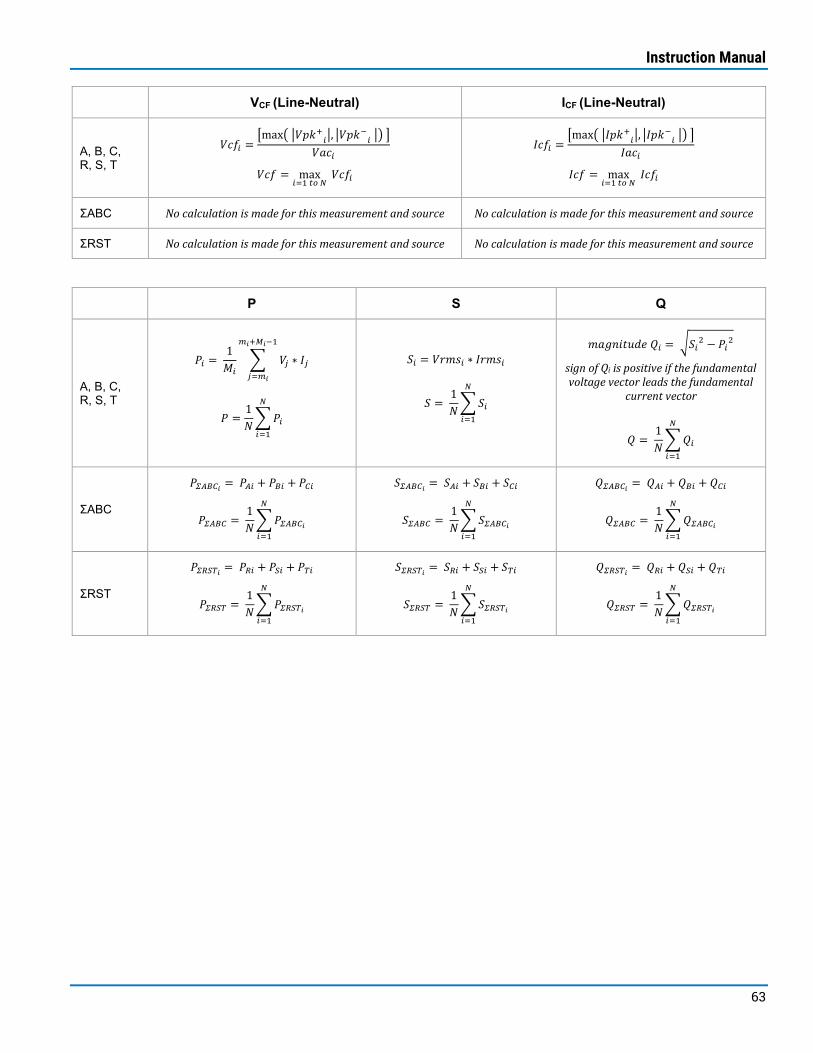
Instruction Manual
63
VCF (Line-Neutral) ICF (Line-Neutral)
A, B, C, R, S, T
𝑉𝑉𝐸𝐸𝑉𝑉𝑖𝑖 =�max� �𝑉𝑉𝑐𝑐𝑉𝑉+𝑖𝑖�, �𝑉𝑉𝑐𝑐𝑉𝑉
−𝑖𝑖 �� �
𝑉𝑉𝐸𝐸𝐸𝐸𝑖𝑖
𝑉𝑉𝐸𝐸𝑉𝑉 = max𝑖𝑖=1 𝑡𝑡𝑡𝑡 𝑁𝑁
𝑉𝑉𝐸𝐸𝑉𝑉𝑖𝑖
𝐼𝐼𝐸𝐸𝑉𝑉𝑖𝑖 =�max� �𝐼𝐼𝑐𝑐𝑉𝑉+𝑖𝑖�, �𝐼𝐼𝑐𝑐𝑉𝑉
−𝑖𝑖 �� �
𝐼𝐼𝐸𝐸𝐸𝐸𝑖𝑖
𝐼𝐼𝐸𝐸𝑉𝑉 = max𝑖𝑖=1 𝑡𝑡𝑡𝑡 𝑁𝑁
𝐼𝐼𝐸𝐸𝑉𝑉𝑖𝑖
ΣABC No calculation is made for this measurement and source No calculation is made for this measurement and source
ΣRST No calculation is made for this measurement and source No calculation is made for this measurement and source
P S Q
A, B, C, R, S, T
𝑃𝑃𝑖𝑖 = 1𝑀𝑀𝑖𝑖
� 𝑉𝑉𝑗𝑗 ∗ 𝐼𝐼𝑗𝑗
𝑚𝑚𝑖𝑖+𝑀𝑀𝑖𝑖−1
𝑗𝑗=𝑚𝑚𝑖𝑖
𝑃𝑃 =1𝑁𝑁�𝑃𝑃𝑖𝑖
𝑁𝑁
𝑖𝑖=1
𝑆𝑆𝑖𝑖 = 𝑉𝑉𝑎𝑎𝑎𝑎𝑉𝑉𝑖𝑖 ∗ 𝐼𝐼𝑎𝑎𝑎𝑎𝑉𝑉𝑖𝑖
𝑆𝑆 = 1𝑁𝑁�𝑆𝑆𝑖𝑖
𝑁𝑁
𝑖𝑖=1
𝑎𝑎𝐸𝐸𝑚𝑚𝑎𝑎𝑎𝑎𝐹𝐹𝐹𝐹𝑜𝑜𝑜𝑜 𝑄𝑄𝑖𝑖 = �𝑆𝑆𝑖𝑖2 − 𝑃𝑃𝑖𝑖2
sign of Qi is positive if the fundamental voltage vector leads the fundamental
current vector
𝑄𝑄 = 1𝑁𝑁�𝑄𝑄𝑖𝑖
𝑁𝑁
𝑖𝑖=1
ΣABC
𝑃𝑃𝛴𝛴𝛴𝛴𝛴𝛴𝛴𝛴𝑖𝑖 = 𝑃𝑃𝛴𝛴𝑖𝑖 + 𝑃𝑃𝛴𝛴𝑖𝑖 + 𝑃𝑃𝛴𝛴𝑖𝑖
𝑃𝑃𝛴𝛴𝛴𝛴𝛴𝛴𝛴𝛴 = 1𝑁𝑁�𝑃𝑃𝛴𝛴𝛴𝛴𝛴𝛴𝛴𝛴𝑖𝑖
𝑁𝑁
𝑖𝑖=1
𝑆𝑆𝛴𝛴𝛴𝛴𝛴𝛴𝛴𝛴𝑖𝑖 = 𝑆𝑆𝛴𝛴𝑖𝑖 + 𝑆𝑆𝛴𝛴𝑖𝑖 + 𝑆𝑆𝛴𝛴𝑖𝑖
𝑆𝑆𝛴𝛴𝛴𝛴𝛴𝛴𝛴𝛴 = 1𝑁𝑁�𝑆𝑆𝛴𝛴𝛴𝛴𝛴𝛴𝛴𝛴𝑖𝑖
𝑁𝑁
𝑖𝑖=1
𝑄𝑄𝛴𝛴𝛴𝛴𝛴𝛴𝛴𝛴𝑖𝑖 = 𝑄𝑄𝛴𝛴𝑖𝑖 + 𝑄𝑄𝛴𝛴𝑖𝑖 + 𝑄𝑄𝛴𝛴𝑖𝑖
𝑄𝑄𝛴𝛴𝛴𝛴𝛴𝛴𝛴𝛴 = 1𝑁𝑁�𝑄𝑄𝛴𝛴𝛴𝛴𝛴𝛴𝛴𝛴𝑖𝑖
𝑁𝑁
𝑖𝑖=1
ΣRST
𝑃𝑃𝛴𝛴𝛴𝛴𝛴𝛴𝛴𝛴𝑖𝑖 = 𝑃𝑃𝛴𝛴𝑖𝑖 + 𝑃𝑃𝛴𝛴𝑖𝑖 + 𝑃𝑃𝛴𝛴𝑖𝑖
𝑃𝑃𝛴𝛴𝛴𝛴𝛴𝛴𝛴𝛴 = 1𝑁𝑁�𝑃𝑃𝛴𝛴𝛴𝛴𝛴𝛴𝛴𝛴𝑖𝑖
𝑁𝑁
𝑖𝑖=1
𝑆𝑆𝛴𝛴𝛴𝛴𝛴𝛴𝛴𝛴𝑖𝑖 = 𝑆𝑆𝛴𝛴𝑖𝑖 + 𝑆𝑆𝛴𝛴𝑖𝑖 + 𝑆𝑆𝛴𝛴𝑖𝑖
𝑆𝑆𝛴𝛴𝛴𝛴𝛴𝛴𝛴𝛴 = 1𝑁𝑁�𝑆𝑆𝛴𝛴𝛴𝛴𝛴𝛴𝛴𝛴𝑖𝑖
𝑁𝑁
𝑖𝑖=1
𝑄𝑄𝛴𝛴𝛴𝛴𝛴𝛴𝛴𝛴𝑖𝑖 = 𝑄𝑄𝛴𝛴𝑖𝑖 + 𝑄𝑄𝛴𝛴𝑖𝑖 + 𝑄𝑄𝛴𝛴𝑖𝑖
𝑄𝑄𝛴𝛴𝛴𝛴𝛴𝛴𝛴𝛴 = 1𝑁𝑁�𝑄𝑄𝛴𝛴𝛴𝛴𝛴𝛴𝛴𝛴𝑖𝑖
𝑁𝑁
𝑖𝑖=1

3-phase Power Analysis Software
64
PPK+, PPK- λ (Power Factor) ϕ (Phase Angle)
A, B, C, R, S, T
𝑃𝑃𝑐𝑐𝑉𝑉⁺𝑖𝑖 = max𝑗𝑗=𝑚𝑚𝑖𝑖 𝑡𝑡𝑡𝑡 𝑚𝑚𝑖𝑖+𝑀𝑀𝑖𝑖−1
𝑉𝑉𝑗𝑗 ∗ 𝐼𝐼𝑗𝑗
𝑃𝑃𝑐𝑐𝑉𝑉⁻𝑖𝑖 = min𝑗𝑗=𝑚𝑚𝑖𝑖 𝑡𝑡𝑡𝑡 𝑚𝑚𝑖𝑖+𝑀𝑀𝑖𝑖−1
𝑉𝑉𝑗𝑗 ∗ 𝐼𝐼𝑗𝑗
𝑃𝑃𝑐𝑐𝑉𝑉+ = max𝑖𝑖=1 𝑡𝑡𝑡𝑡 𝑁𝑁
𝑃𝑃𝑐𝑐𝑉𝑉⁺𝑖𝑖
𝑃𝑃𝑐𝑐𝑉𝑉⁻ = min𝑖𝑖=1 𝑡𝑡𝑡𝑡 𝑁𝑁
𝑃𝑃𝑐𝑐𝑉𝑉⁻𝑖𝑖
𝜆𝜆𝑖𝑖 = 𝑃𝑃𝑖𝑖𝑆𝑆𝑖𝑖
𝜆𝜆 = 1𝑁𝑁�𝜆𝜆𝑖𝑖
𝑁𝑁
𝑖𝑖=1
𝑎𝑎𝐸𝐸𝑚𝑚𝑎𝑎𝑎𝑎𝐹𝐹𝐹𝐹𝑜𝑜𝑜𝑜 𝜙𝜙𝑖𝑖 = cos−1 𝜆𝜆𝑖𝑖
sign of ϕi is positive if the fundamental voltage vector
leads the fundamental current vector
𝜙𝜙 = 1𝑁𝑁�𝜙𝜙𝑖𝑖
𝑁𝑁
𝑖𝑖=1
ΣABC
𝑃𝑃𝑐𝑐𝑉𝑉+𝛴𝛴𝛴𝛴𝛴𝛴𝛴𝛴𝑖𝑖 = max�𝑉𝑉𝛴𝛴𝑗𝑗 ∗ 𝐼𝐼𝛴𝛴𝑗𝑗 + 𝑉𝑉𝛴𝛴𝑗𝑗 ∗ 𝐼𝐼𝛴𝛴𝑗𝑗 + 𝑉𝑉𝛴𝛴𝑗𝑗 ∗ 𝐼𝐼𝛴𝛴𝑗𝑗�
𝑃𝑃𝑐𝑐𝑉𝑉⁻𝛴𝛴𝛴𝛴𝛴𝛴𝛴𝛴𝑖𝑖 = min�𝑉𝑉𝛴𝛴𝑗𝑗 ∗ 𝐼𝐼𝛴𝛴𝑗𝑗 + 𝑉𝑉𝛴𝛴𝑗𝑗 ∗ 𝐼𝐼𝛴𝛴𝑗𝑗 + 𝑉𝑉𝛴𝛴𝑗𝑗 ∗ 𝐼𝐼𝛴𝛴𝑗𝑗�
𝑃𝑃𝑐𝑐𝑉𝑉+𝛴𝛴𝛴𝛴𝛴𝛴𝛴𝛴 = max𝑖𝑖=1 𝑡𝑡𝑡𝑡 𝑁𝑁
𝑃𝑃𝑐𝑐𝑉𝑉+𝛴𝛴𝛴𝛴𝛴𝛴𝛴𝛴𝑖𝑖
𝑃𝑃𝑐𝑐𝑉𝑉⁻𝛴𝛴𝛴𝛴𝛴𝛴𝛴𝛴 = max𝑖𝑖=1 𝑡𝑡𝑡𝑡 𝑁𝑁
𝑃𝑃𝑐𝑐𝑉𝑉⁻𝛴𝛴𝛴𝛴𝛴𝛴𝛴𝛴𝑖𝑖
𝜆𝜆𝛴𝛴𝛴𝛴𝛴𝛴𝛴𝛴𝑖𝑖 = 13 (𝜆𝜆𝛴𝛴𝑖𝑖 + 𝜆𝜆𝛴𝛴𝑖𝑖 + 𝜆𝜆𝛴𝛴𝑖𝑖)
𝜆𝜆𝛴𝛴𝛴𝛴𝛴𝛴𝛴𝛴 = 1𝑁𝑁 �𝜆𝜆𝛴𝛴𝛴𝛴𝛴𝛴𝛴𝛴𝑖𝑖
𝑁𝑁
𝑖𝑖=1
𝜙𝜙𝛴𝛴𝛴𝛴𝛴𝛴𝛴𝛴𝑖𝑖 = 13 (𝜙𝜙𝛴𝛴𝑖𝑖 + 𝜙𝜙𝛴𝛴𝑖𝑖 + 𝜙𝜙𝛴𝛴𝑖𝑖)
𝜙𝜙𝛴𝛴𝛴𝛴𝛴𝛴𝛴𝛴 = 1𝑁𝑁 �𝜙𝜙𝛴𝛴𝛴𝛴𝛴𝛴𝛴𝛴𝑖𝑖
𝑁𝑁
𝑖𝑖=1
ΣRST
𝑃𝑃𝑐𝑐𝑉𝑉+𝛴𝛴𝛴𝛴𝛴𝛴𝛴𝛴𝑖𝑖 = max�𝑉𝑉𝛴𝛴𝑗𝑗 ∗ 𝐼𝐼𝛴𝛴𝑗𝑗 + 𝑉𝑉𝛴𝛴𝑗𝑗 ∗ 𝐼𝐼𝛴𝛴𝑗𝑗 + 𝑉𝑉𝛴𝛴𝑗𝑗 ∗ 𝐼𝐼𝛴𝛴𝑗𝑗�
𝑃𝑃𝑐𝑐𝑉𝑉⁻𝛴𝛴𝛴𝛴𝛴𝛴𝛴𝛴𝑖𝑖 = min�𝑉𝑉𝛴𝛴𝑗𝑗 ∗ 𝐼𝐼𝛴𝛴𝑗𝑗 + 𝑉𝑉𝛴𝛴𝑗𝑗 ∗ 𝐼𝐼𝛴𝛴𝑗𝑗 + 𝑉𝑉𝛴𝛴𝑗𝑗 ∗ 𝐼𝐼𝛴𝛴𝑗𝑗�
𝑃𝑃𝑐𝑐𝑉𝑉+𝛴𝛴𝛴𝛴𝛴𝛴𝛴𝛴 = max𝑖𝑖=1 𝑡𝑡𝑡𝑡 𝑁𝑁
𝑃𝑃𝑐𝑐𝑉𝑉+𝛴𝛴𝛴𝛴𝛴𝛴𝛴𝛴𝑖𝑖
𝑃𝑃𝑐𝑐𝑉𝑉⁻𝛴𝛴𝛴𝛴𝛴𝛴𝛴𝛴 = max𝑖𝑖=1 𝑡𝑡𝑡𝑡 𝑁𝑁
𝑃𝑃𝑐𝑐𝑉𝑉⁻𝛴𝛴𝛴𝛴𝛴𝛴𝛴𝛴𝑖𝑖
𝜆𝜆𝛴𝛴𝛴𝛴𝛴𝛴𝛴𝛴𝑖𝑖 = 13 (𝜆𝜆𝛴𝛴𝑖𝑖 + 𝜆𝜆𝛴𝛴𝑖𝑖 + 𝜆𝜆𝛴𝛴𝑖𝑖)
𝜆𝜆𝛴𝛴𝛴𝛴𝛴𝛴𝛴𝛴 = 1𝑁𝑁 �𝜆𝜆𝛴𝛴𝛴𝛴𝛴𝛴𝛴𝛴𝑖𝑖
𝑁𝑁
𝑖𝑖=1
𝜙𝜙𝛴𝛴𝛴𝛴𝛴𝛴𝛴𝛴𝑖𝑖 = 13 (𝜙𝜙𝛴𝛴𝑖𝑖 + 𝜙𝜙𝛴𝛴𝑖𝑖 + 𝜙𝜙𝛴𝛴𝑖𝑖)
𝜙𝜙𝛴𝛴𝛴𝛴𝛴𝛴𝛴𝛴 = 1𝑁𝑁 �𝜙𝜙𝛴𝛴𝛴𝛴𝛴𝛴𝛴𝛴𝑖𝑖
𝑁𝑁
𝑖𝑖=1
Slip Stage-Stage Efficiency (η1) Cumulative Efficiency (η2)
ΣABC DC Bus ΣRST
𝑆𝑆𝐹𝐹𝑎𝑎𝑐𝑐𝑖𝑖 = 1𝑀𝑀𝑖𝑖
� �𝜔𝜔𝑉𝑉𝑗𝑗 − 𝜔𝜔𝑗𝑗
𝜔𝜔𝑗𝑗�
𝑚𝑚𝑖𝑖+𝑀𝑀𝑖𝑖−1
𝑗𝑗=𝑚𝑚𝑖𝑖
ωsj is the instantaneous speed calculation of the stator magnetic field.
ωsj and ωj are calculated internally and are not displayed.
𝑆𝑆𝐹𝐹𝑎𝑎𝑐𝑐 = 1𝑁𝑁�𝑆𝑆𝐹𝐹𝑎𝑎𝑐𝑐𝑖𝑖
𝑁𝑁
𝑖𝑖=1
𝜂𝜂1𝑖𝑖 = �𝑃𝑃𝛴𝛴𝛴𝛴𝛴𝛴𝑆𝑆𝑆𝑆2𝑖𝑖𝑃𝑃𝛴𝛴𝛴𝛴𝛴𝛴𝑆𝑆𝑆𝑆1𝑖𝑖
� ∗ 100%
𝑁𝑁𝐹𝐹𝑎𝑎𝑜𝑜𝑎𝑎𝑎𝑎𝐸𝐸 𝐹𝐹𝐸𝐸𝑡𝑡𝐹𝐹𝑜𝑜 𝑣𝑣𝐸𝐸𝐹𝐹𝐹𝐹𝑜𝑜𝑉𝑉1𝑁𝑁�𝜂𝜂1𝑖𝑖
𝑁𝑁
𝑖𝑖=1
In the event of unequal sync cycle periods, a new efficiency value will be
calculated on each cyclic positive transition.
𝜂𝜂2𝑖𝑖 = �𝑃𝑃𝐿𝐿𝛴𝛴𝛴𝛴𝛴𝛴𝑖𝑖𝑃𝑃𝐹𝐹𝐹𝐹𝛴𝛴𝛴𝛴𝛴𝛴𝑖𝑖
� ∗ 100%
𝑁𝑁𝐹𝐹𝑎𝑎𝑜𝑜𝑎𝑎𝑎𝑎𝐸𝐸 𝐹𝐹𝐸𝐸𝑡𝑡𝐹𝐹𝑜𝑜 𝑣𝑣𝐸𝐸𝐹𝐹𝐹𝐹𝑜𝑜𝑉𝑉1𝑁𝑁�𝜂𝜂2𝑖𝑖
𝑁𝑁
𝑖𝑖=1
In the event of unequal sync cycle periods, a new efficiency value will be
calculated on each cyclic positive transition.
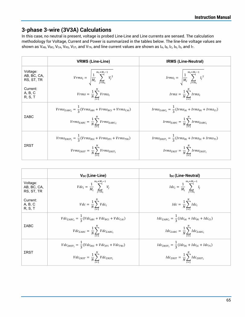
Instruction Manual
65
3-phase 3-wire (3V3A) Calculations In this case, no neutral is present, voltage is probed Line-Line and Line currents are sensed. The calculation methodology for Voltage, Current and Power is summarized in the tables below. The line-line voltage values are shown as VAB, VBC, VCA, VRS, VST, and VTR, and line current values are shown as IA, IB, IC, IR, IS, and IT.
VRMS (Line-Line) IRMS (Line-Neutral)
Voltage: AB, BC, CA, RS, ST, TR
Current: A, B, C R, S, T
𝑉𝑉𝑎𝑎𝑎𝑎𝑉𝑉𝑖𝑖 = �1𝑀𝑀𝑖𝑖
� 𝑉𝑉𝑗𝑗2𝑚𝑚𝑖𝑖+𝑀𝑀𝑖𝑖−1
𝑗𝑗=𝑚𝑚𝑖𝑖
𝑉𝑉𝑎𝑎𝑎𝑎𝑉𝑉 = 1𝑁𝑁�𝑉𝑉𝑎𝑎𝑎𝑎𝑉𝑉𝑖𝑖
𝑁𝑁
𝑖𝑖=1
𝐼𝐼𝑎𝑎𝑎𝑎𝑉𝑉𝑖𝑖 = �1𝑀𝑀𝑖𝑖
� 𝐼𝐼𝑗𝑗2𝑚𝑚𝑖𝑖+𝑀𝑀𝑖𝑖−1
𝑗𝑗=𝑚𝑚𝑖𝑖
𝐼𝐼𝑎𝑎𝑎𝑎𝑉𝑉 = 1𝑁𝑁�𝐼𝐼𝑎𝑎𝑎𝑎𝑉𝑉𝑖𝑖
𝑁𝑁
𝑖𝑖=1
ΣABC
𝑉𝑉𝑎𝑎𝑎𝑎𝑉𝑉𝛴𝛴𝛴𝛴𝛴𝛴𝛴𝛴𝑖𝑖 = 13
(𝑉𝑉𝑎𝑎𝑎𝑎𝑉𝑉𝛴𝛴𝛴𝛴𝑖𝑖 + 𝑉𝑉𝑎𝑎𝑎𝑎𝑉𝑉𝛴𝛴𝛴𝛴𝑖𝑖 + 𝑉𝑉𝑎𝑎𝑎𝑎𝑉𝑉𝛴𝛴𝛴𝛴𝑖𝑖)
𝑉𝑉𝑎𝑎𝑎𝑎𝑉𝑉𝛴𝛴𝛴𝛴𝛴𝛴𝛴𝛴 = 1𝑁𝑁�𝑉𝑉𝑎𝑎𝑎𝑎𝑉𝑉𝛴𝛴𝛴𝛴𝛴𝛴𝛴𝛴𝑖𝑖
𝑁𝑁
𝑖𝑖=1
𝐼𝐼𝑎𝑎𝑎𝑎𝑉𝑉𝛴𝛴𝛴𝛴𝛴𝛴𝛴𝛴𝑖𝑖 = 13
(𝐼𝐼𝑎𝑎𝑎𝑎𝑉𝑉𝛴𝛴𝑖𝑖 + 𝐼𝐼𝑎𝑎𝑎𝑎𝑉𝑉𝛴𝛴𝑖𝑖 + 𝐼𝐼𝑎𝑎𝑎𝑎𝑉𝑉𝛴𝛴𝑖𝑖)
𝐼𝐼𝑎𝑎𝑎𝑎𝑉𝑉𝛴𝛴𝛴𝛴𝛴𝛴𝛴𝛴 = 1𝑁𝑁�𝐼𝐼𝑎𝑎𝑎𝑎𝑉𝑉𝛴𝛴𝛴𝛴𝛴𝛴𝛴𝛴𝑖𝑖
𝑁𝑁
𝑖𝑖=1
ΣRST
𝑉𝑉𝑎𝑎𝑎𝑎𝑉𝑉𝛴𝛴𝛴𝛴𝛴𝛴𝛴𝛴𝑖𝑖 = 13
(𝑉𝑉𝑎𝑎𝑎𝑎𝑉𝑉𝛴𝛴𝛴𝛴𝑖𝑖 + 𝑉𝑉𝑎𝑎𝑎𝑎𝑉𝑉𝛴𝛴𝛴𝛴𝑖𝑖 + 𝑉𝑉𝑎𝑎𝑎𝑎𝑉𝑉𝛴𝛴𝛴𝛴𝑖𝑖)
𝑉𝑉𝑎𝑎𝑎𝑎𝑉𝑉𝛴𝛴𝛴𝛴𝛴𝛴𝛴𝛴 = 1𝑁𝑁�𝑉𝑉𝑎𝑎𝑎𝑎𝑉𝑉𝛴𝛴𝛴𝛴𝛴𝛴𝛴𝛴𝑖𝑖
𝑁𝑁
𝑖𝑖=1
𝐼𝐼𝑎𝑎𝑎𝑎𝑉𝑉𝛴𝛴𝛴𝛴𝛴𝛴𝛴𝛴𝑖𝑖 = 13
(𝐼𝐼𝑎𝑎𝑎𝑎𝑉𝑉𝛴𝛴𝑖𝑖 + 𝐼𝐼𝑎𝑎𝑎𝑎𝑉𝑉𝛴𝛴𝑖𝑖 + 𝐼𝐼𝑎𝑎𝑎𝑎𝑉𝑉𝛴𝛴𝑖𝑖)
𝐼𝐼𝑎𝑎𝑎𝑎𝑉𝑉𝛴𝛴𝛴𝛴𝛴𝛴𝛴𝛴 = 1𝑁𝑁�𝐼𝐼𝑎𝑎𝑎𝑎𝑉𝑉𝛴𝛴𝛴𝛴𝛴𝛴𝛴𝛴𝑖𝑖
𝑁𝑁
𝑖𝑖=1
VDC (Line-Line) IDC (Line-Neutral)
Voltage: AB, BC, CA, RS, ST, TR
Current: A, B, C R, S, T
𝑉𝑉𝑜𝑜𝐸𝐸𝑖𝑖 = 1𝑀𝑀𝑖𝑖
� 𝑉𝑉𝑗𝑗
𝑚𝑚𝑖𝑖+𝑀𝑀𝑖𝑖−1
𝑗𝑗=𝑚𝑚𝑖𝑖
𝑉𝑉𝑜𝑜𝐸𝐸 = 1𝑁𝑁�𝑉𝑉𝑜𝑜𝐸𝐸𝑖𝑖
𝑁𝑁
𝑖𝑖=1
𝐼𝐼𝑜𝑜𝐸𝐸𝑖𝑖 = 1𝑀𝑀𝑖𝑖
� 𝐼𝐼𝑗𝑗
𝑚𝑚𝑖𝑖+𝑀𝑀𝑖𝑖−1
𝑗𝑗=𝑚𝑚𝑖𝑖
𝐼𝐼𝑜𝑜𝐸𝐸 = 1𝑁𝑁�𝐼𝐼𝑜𝑜𝐸𝐸𝑖𝑖
𝑁𝑁
𝑖𝑖=1
ΣABC
𝑉𝑉𝑜𝑜𝐸𝐸𝛴𝛴𝛴𝛴𝛴𝛴𝛴𝛴𝑖𝑖 = 13
(𝑉𝑉𝑜𝑜𝐸𝐸𝛴𝛴𝛴𝛴𝑖𝑖 + 𝑉𝑉𝑜𝑜𝐸𝐸𝛴𝛴𝛴𝛴𝑖𝑖 + 𝑉𝑉𝑜𝑜𝐸𝐸𝛴𝛴𝛴𝛴𝑖𝑖)
𝑉𝑉𝑜𝑜𝐸𝐸𝛴𝛴𝛴𝛴𝛴𝛴𝛴𝛴 = 1𝑁𝑁�𝑉𝑉𝑜𝑜𝐸𝐸𝛴𝛴𝛴𝛴𝛴𝛴𝛴𝛴𝑖𝑖
𝑁𝑁
𝑖𝑖=1
𝐼𝐼𝑜𝑜𝐸𝐸𝛴𝛴𝛴𝛴𝛴𝛴𝛴𝛴𝑖𝑖 = 13
(𝐼𝐼𝑜𝑜𝐸𝐸𝛴𝛴𝑖𝑖 + 𝐼𝐼𝑜𝑜𝐸𝐸𝛴𝛴𝑖𝑖 + 𝐼𝐼𝑜𝑜𝐸𝐸𝛴𝛴𝑖𝑖)
𝐼𝐼𝑜𝑜𝐸𝐸𝛴𝛴𝛴𝛴𝛴𝛴𝛴𝛴 = 1𝑁𝑁�𝐼𝐼𝑜𝑜𝐸𝐸𝛴𝛴𝛴𝛴𝛴𝛴𝛴𝛴𝑖𝑖
𝑁𝑁
𝑖𝑖=1
ΣRST
𝑉𝑉𝑜𝑜𝐸𝐸𝛴𝛴𝛴𝛴𝛴𝛴𝛴𝛴𝑖𝑖 = 13
(𝑉𝑉𝑜𝑜𝐸𝐸𝛴𝛴𝛴𝛴𝑖𝑖 + 𝑉𝑉𝑜𝑜𝐸𝐸𝛴𝛴𝛴𝛴𝑖𝑖 + 𝑉𝑉𝑜𝑜𝐸𝐸𝛴𝛴𝛴𝛴𝑖𝑖)
𝑉𝑉𝑜𝑜𝐸𝐸𝛴𝛴𝛴𝛴𝛴𝛴𝛴𝛴 = 1𝑁𝑁�𝑉𝑉𝑜𝑜𝐸𝐸𝛴𝛴𝛴𝛴𝛴𝛴𝛴𝛴𝑖𝑖
𝑁𝑁
𝑖𝑖=1
𝐼𝐼𝑜𝑜𝐸𝐸𝛴𝛴𝛴𝛴𝛴𝛴𝛴𝛴𝑖𝑖 = 13
(𝐼𝐼𝑜𝑜𝐸𝐸𝛴𝛴𝑖𝑖 + 𝐼𝐼𝑜𝑜𝐸𝐸𝛴𝛴𝑖𝑖 + 𝐼𝐼𝑜𝑜𝐸𝐸𝛴𝛴𝑖𝑖)
𝐼𝐼𝑜𝑜𝐸𝐸𝛴𝛴𝛴𝛴𝛴𝛴𝛴𝛴 = 1𝑁𝑁�𝐼𝐼𝑜𝑜𝐸𝐸𝛴𝛴𝛴𝛴𝛴𝛴𝛴𝛴𝑖𝑖
𝑁𝑁
𝑖𝑖=1

3-phase Power Analysis Software
66
VAC (Line-Line) IAC (Line-Neutral)
Voltage: AB, BC, CA, RS, ST, TR
Current: A, B, C R, S, T
𝑉𝑉𝐸𝐸𝐸𝐸𝑖𝑖 = 𝑉𝑉𝑎𝑎𝑎𝑎𝑉𝑉𝑖𝑖 − 𝑉𝑉𝑜𝑜𝐸𝐸𝑖𝑖
𝑉𝑉𝐸𝐸𝐸𝐸 = 1𝑁𝑁�𝑉𝑉𝐸𝐸𝐸𝐸𝑖𝑖
𝑁𝑁
𝑖𝑖=1
𝐼𝐼𝐸𝐸𝐸𝐸𝑖𝑖 = 𝐼𝐼𝑎𝑎𝑎𝑎𝑉𝑉𝑖𝑖 − 𝐼𝐼𝑜𝑜𝐸𝐸𝑖𝑖
𝐼𝐼𝐸𝐸𝐸𝐸 = 1𝑁𝑁�𝐼𝐼𝐸𝐸𝐸𝐸𝑖𝑖
𝑁𝑁
𝑖𝑖=1
ΣABC
𝑉𝑉𝐸𝐸𝐸𝐸𝛴𝛴𝛴𝛴𝛴𝛴𝛴𝛴𝑖𝑖 = 13
(𝑉𝑉𝐸𝐸𝐸𝐸𝛴𝛴𝛴𝛴𝑖𝑖 + 𝑉𝑉𝐸𝐸𝐸𝐸𝛴𝛴𝛴𝛴𝑖𝑖 + 𝑉𝑉𝐸𝐸𝐸𝐸𝛴𝛴𝛴𝛴𝑖𝑖)
𝑉𝑉𝐸𝐸𝐸𝐸𝛴𝛴𝛴𝛴𝛴𝛴𝛴𝛴 = 1𝑁𝑁�𝑉𝑉𝐸𝐸𝐸𝐸𝛴𝛴𝛴𝛴𝛴𝛴𝛴𝛴𝑖𝑖
𝑁𝑁
𝑖𝑖=1
𝐼𝐼𝐸𝐸𝐸𝐸𝛴𝛴𝛴𝛴𝛴𝛴𝛴𝛴𝑖𝑖 = 13
(𝐼𝐼𝐸𝐸𝐸𝐸𝛴𝛴𝑖𝑖 + 𝐼𝐼𝐸𝐸𝐸𝐸𝛴𝛴𝑖𝑖 + 𝐼𝐼𝐸𝐸𝐸𝐸𝛴𝛴𝑖𝑖)
𝐼𝐼𝐸𝐸𝐸𝐸𝛴𝛴𝛴𝛴𝛴𝛴𝛴𝛴 = 1𝑁𝑁�𝐼𝐼𝐸𝐸𝐸𝐸𝛴𝛴𝛴𝛴𝛴𝛴𝛴𝛴𝑖𝑖
𝑁𝑁
𝑖𝑖=1
ΣRST
𝑉𝑉𝐸𝐸𝐸𝐸𝛴𝛴𝛴𝛴𝛴𝛴𝛴𝛴𝑖𝑖 = 13
(𝑉𝑉𝐸𝐸𝐸𝐸𝛴𝛴𝛴𝛴𝑖𝑖 + 𝑉𝑉𝐸𝐸𝐸𝐸𝛴𝛴𝛴𝛴𝑖𝑖 + 𝑉𝑉𝐸𝐸𝐸𝐸𝛴𝛴𝛴𝛴𝑖𝑖)
𝑉𝑉𝐸𝐸𝐸𝐸𝛴𝛴𝛴𝛴𝛴𝛴𝛴𝛴 = 1𝑁𝑁�𝑉𝑉𝐸𝐸𝐸𝐸𝛴𝛴𝛴𝛴𝛴𝛴𝛴𝛴𝑖𝑖
𝑁𝑁
𝑖𝑖=1
𝐼𝐼𝐸𝐸𝐸𝐸𝛴𝛴𝛴𝛴𝛴𝛴𝛴𝛴𝑖𝑖 = 13
(𝐼𝐼𝐸𝐸𝐸𝐸𝛴𝛴𝑖𝑖 + 𝐼𝐼𝐸𝐸𝐸𝐸𝛴𝛴𝑖𝑖 + 𝐼𝐼𝐸𝐸𝐸𝐸𝛴𝛴𝑖𝑖)
𝐼𝐼𝐸𝐸𝐸𝐸𝛴𝛴𝛴𝛴𝛴𝛴𝛴𝛴 = 1𝑁𝑁�𝐼𝐼𝐸𝐸𝐸𝐸𝛴𝛴𝛴𝛴𝛴𝛴𝛴𝛴𝑖𝑖
𝑁𝑁
𝑖𝑖=1
VPK+, VPK-, VPK-PK (Line-Line) IPK+, IPK-, IPK-PK (Line-Neutral)
Voltage: AB, BC, CA, RS, ST, TR
Current: A, B, C R, S, T
𝑉𝑉𝑐𝑐𝑉𝑉⁺𝑖𝑖 = max𝑗𝑗=𝑚𝑚𝑖𝑖 𝑡𝑡𝑡𝑡 𝑚𝑚𝑖𝑖+𝑀𝑀𝑖𝑖−1
𝑉𝑉𝑗𝑗
𝑉𝑉𝑐𝑐𝑉𝑉⁻𝑖𝑖 = min𝑗𝑗=𝑚𝑚𝑖𝑖 𝑡𝑡𝑡𝑡 𝑚𝑚𝑖𝑖+𝑀𝑀𝑖𝑖−1
𝑉𝑉𝑗𝑗
𝑉𝑉𝑐𝑐𝑉𝑉⎼𝑐𝑐𝑉𝑉𝑖𝑖 = 𝑉𝑉𝑐𝑐𝑉𝑉⁺𝑖𝑖 − 𝑉𝑉𝑐𝑐𝑉𝑉⁻𝑖𝑖 𝑉𝑉𝑐𝑐𝑉𝑉+ = max
𝑖𝑖=1 𝑡𝑡𝑡𝑡 𝑁𝑁 𝑉𝑉𝑐𝑐𝑉𝑉⁺𝑖𝑖
𝑉𝑉𝑐𝑐𝑉𝑉⁻ = min𝑖𝑖=1 𝑡𝑡𝑡𝑡 𝑁𝑁
𝑉𝑉𝑐𝑐𝑉𝑉⁻𝑖𝑖
𝑉𝑉𝑐𝑐𝑉𝑉⎼𝑐𝑐𝑉𝑉 = max𝑖𝑖=1 𝑡𝑡𝑡𝑡 𝑁𝑁
𝑉𝑉𝑐𝑐𝑉𝑉⎼𝑐𝑐𝑉𝑉𝑖𝑖
𝐼𝐼𝑐𝑐𝑉𝑉⁺𝑖𝑖 = max𝑗𝑗=𝑚𝑚𝑖𝑖 𝑡𝑡𝑡𝑡 𝑚𝑚𝑖𝑖+𝑀𝑀𝑖𝑖−1
𝐼𝐼𝑗𝑗
𝐼𝐼𝑐𝑐𝑉𝑉⁻𝑖𝑖 = min𝑗𝑗=𝑚𝑚𝑖𝑖 𝑡𝑡𝑡𝑡 𝑚𝑚𝑖𝑖+𝑀𝑀𝑖𝑖−1
𝐼𝐼𝑗𝑗
𝐼𝐼𝑐𝑐𝑉𝑉⎼𝑐𝑐𝑉𝑉𝑖𝑖 = 𝐼𝐼𝑐𝑐𝑉𝑉⁺𝑖𝑖 − 𝐼𝐼𝑐𝑐𝑉𝑉⁻𝑖𝑖 𝐼𝐼𝑐𝑐𝑉𝑉+ = max
𝑖𝑖=1 𝑡𝑡𝑡𝑡 𝑁𝑁 𝐼𝐼𝑐𝑐𝑉𝑉⁺𝑖𝑖
𝐼𝐼𝑐𝑐𝑉𝑉⁻ = min𝑖𝑖=1 𝑡𝑡𝑡𝑡 𝑁𝑁
𝐼𝐼𝑐𝑐𝑉𝑉⁻𝑖𝑖
𝐼𝐼𝑐𝑐𝑉𝑉⎼𝑐𝑐𝑉𝑉 = max𝑖𝑖=1 𝑡𝑡𝑡𝑡 𝑁𝑁
𝐼𝐼𝑐𝑐𝑉𝑉⎼𝑐𝑐𝑉𝑉𝑖𝑖
ΣABC
𝑉𝑉𝑐𝑐𝑉𝑉+𝛴𝛴𝛴𝛴𝛴𝛴𝛴𝛴𝑖𝑖 = max�𝑉𝑉𝑐𝑐𝑉𝑉+𝛴𝛴𝛴𝛴𝑖𝑖 ,𝑉𝑉𝑐𝑐𝑉𝑉+𝛴𝛴𝛴𝛴𝑖𝑖 ,𝑉𝑉𝑐𝑐𝑉𝑉
+𝛴𝛴𝛴𝛴𝑖𝑖�
𝑉𝑉𝑐𝑐𝑉𝑉⁻𝛴𝛴𝛴𝛴𝛴𝛴𝛴𝛴𝑖𝑖 = min�𝑉𝑉𝑐𝑐𝑉𝑉⁻𝛴𝛴𝛴𝛴𝑖𝑖 ,𝑉𝑉𝑐𝑐𝑉𝑉⁻𝛴𝛴𝛴𝛴𝑖𝑖 ,𝑉𝑉𝑐𝑐𝑉𝑉
⁻𝛴𝛴𝛴𝛴𝑖𝑖�
𝑉𝑉𝑐𝑐𝑉𝑉⎼𝑐𝑐𝑉𝑉𝛴𝛴𝛴𝛴𝛴𝛴𝛴𝛴𝑖𝑖 = max(𝑉𝑉𝑐𝑐𝑉𝑉⎼𝑐𝑐𝑉𝑉𝛴𝛴𝛴𝛴𝑖𝑖 ,𝑉𝑉𝑐𝑐𝑉𝑉⎼𝑐𝑐𝑉𝑉𝛴𝛴𝛴𝛴𝑖𝑖 ,𝑉𝑉𝑐𝑐𝑉𝑉⎼𝑐𝑐𝑉𝑉𝛴𝛴𝛴𝛴𝑖𝑖) 𝑉𝑉𝑐𝑐𝑉𝑉+𝛴𝛴𝛴𝛴𝛴𝛴𝛴𝛴 = max
𝑖𝑖=1 𝑡𝑡𝑡𝑡 𝑁𝑁 𝑉𝑉𝑐𝑐𝑉𝑉+𝛴𝛴𝛴𝛴𝛴𝛴𝛴𝛴𝑖𝑖
𝑉𝑉𝑐𝑐𝑉𝑉⁻𝛴𝛴𝛴𝛴𝛴𝛴𝛴𝛴 = min𝑖𝑖=1 𝑡𝑡𝑡𝑡 𝑁𝑁
𝑉𝑉𝑐𝑐𝑉𝑉⁻𝛴𝛴𝛴𝛴𝛴𝛴𝛴𝛴𝑖𝑖
𝑉𝑉𝑐𝑐𝑉𝑉⎼𝑐𝑐𝑉𝑉𝛴𝛴𝛴𝛴𝛴𝛴𝛴𝛴 = max𝑖𝑖=1 𝑡𝑡𝑡𝑡 𝑁𝑁
𝑉𝑉𝑐𝑐𝑉𝑉⎼𝑐𝑐𝑉𝑉𝛴𝛴𝛴𝛴𝛴𝛴𝛴𝛴𝑖𝑖
𝐼𝐼𝑐𝑐𝑉𝑉+𝛴𝛴𝛴𝛴𝛴𝛴𝛴𝛴𝑖𝑖 = max�𝐼𝐼𝑐𝑐𝑉𝑉+𝛴𝛴𝑖𝑖 , 𝐼𝐼𝑐𝑐𝑉𝑉+𝛴𝛴𝑖𝑖 , 𝐼𝐼𝑐𝑐𝑉𝑉
+𝛴𝛴𝑖𝑖�
𝐼𝐼𝑐𝑐𝑉𝑉⁻𝛴𝛴𝛴𝛴𝛴𝛴𝛴𝛴𝑖𝑖 = min�𝐼𝐼𝑐𝑐𝑉𝑉⁻𝛴𝛴𝑖𝑖 , 𝐼𝐼𝑐𝑐𝑉𝑉⁻𝛴𝛴𝑖𝑖 , 𝐼𝐼𝑐𝑐𝑉𝑉
⁻𝛴𝛴𝑖𝑖�
𝐼𝐼𝑐𝑐𝑉𝑉⎼𝑐𝑐𝑉𝑉𝛴𝛴𝛴𝛴𝛴𝛴𝛴𝛴𝑖𝑖 = max(𝐼𝐼𝑐𝑐𝑉𝑉⎼𝑐𝑐𝑉𝑉𝛴𝛴𝑖𝑖 , 𝐼𝐼𝑐𝑐𝑉𝑉⎼𝑐𝑐𝑉𝑉𝛴𝛴𝑖𝑖 , 𝐼𝐼𝑐𝑐𝑉𝑉⎼𝑐𝑐𝑉𝑉𝛴𝛴𝑖𝑖) 𝐼𝐼𝑐𝑐𝑉𝑉+𝛴𝛴𝛴𝛴𝛴𝛴𝛴𝛴 = max
𝑖𝑖=1 𝑡𝑡𝑡𝑡 𝑁𝑁 𝐼𝐼𝑐𝑐𝑉𝑉+𝛴𝛴𝛴𝛴𝛴𝛴𝛴𝛴𝑖𝑖
𝐼𝐼𝑐𝑐𝑉𝑉⁻𝛴𝛴𝛴𝛴𝛴𝛴𝛴𝛴 = min𝑖𝑖=1 𝑡𝑡𝑡𝑡 𝑁𝑁
𝐼𝐼𝑐𝑐𝑉𝑉⁻𝛴𝛴𝛴𝛴𝛴𝛴𝛴𝛴𝑖𝑖
𝐼𝐼𝑐𝑐𝑉𝑉⎼𝑐𝑐𝑉𝑉𝛴𝛴𝛴𝛴𝛴𝛴𝛴𝛴 = max𝑖𝑖=1 𝑡𝑡𝑡𝑡 𝑁𝑁
𝐼𝐼𝑐𝑐𝑉𝑉⎼𝑐𝑐𝑉𝑉𝛴𝛴𝛴𝛴𝛴𝛴𝛴𝛴𝑖𝑖
ΣRST
𝑉𝑉𝑐𝑐𝑉𝑉+𝛴𝛴𝛴𝛴𝛴𝛴𝛴𝛴𝑖𝑖 = max�𝑉𝑉𝑐𝑐𝑉𝑉+𝛴𝛴𝛴𝛴𝑖𝑖 ,𝑉𝑉𝑐𝑐𝑉𝑉+𝛴𝛴𝛴𝛴𝑖𝑖 ,𝑉𝑉𝑐𝑐𝑉𝑉
+𝛴𝛴𝛴𝛴𝑖𝑖�
𝑉𝑉𝑐𝑐𝑉𝑉⁻𝛴𝛴𝛴𝛴𝛴𝛴𝛴𝛴𝑖𝑖 = min�𝑉𝑉𝑐𝑐𝑉𝑉⁻𝛴𝛴𝛴𝛴𝑖𝑖 ,𝑉𝑉𝑐𝑐𝑉𝑉⁻𝛴𝛴𝛴𝛴𝑖𝑖 ,𝑉𝑉𝑐𝑐𝑉𝑉
⁻𝛴𝛴𝛴𝛴𝑖𝑖�
𝑉𝑉𝑐𝑐𝑉𝑉⎼𝑐𝑐𝑉𝑉𝛴𝛴𝛴𝛴𝛴𝛴𝛴𝛴𝑖𝑖 = max(𝑉𝑉𝑐𝑐𝑉𝑉⎼𝑐𝑐𝑉𝑉𝛴𝛴𝛴𝛴𝑖𝑖 ,𝑉𝑉𝑐𝑐𝑉𝑉⎼𝑐𝑐𝑉𝑉𝛴𝛴𝛴𝛴𝑖𝑖 ,𝑉𝑉𝑐𝑐𝑉𝑉⎼𝑐𝑐𝑉𝑉𝛴𝛴𝛴𝛴𝑖𝑖) 𝑉𝑉𝑐𝑐𝑉𝑉+𝛴𝛴𝛴𝛴𝛴𝛴𝛴𝛴 = max
𝑖𝑖=1 𝑡𝑡𝑡𝑡 𝑁𝑁 𝑉𝑉𝑐𝑐𝑉𝑉+𝛴𝛴𝛴𝛴𝛴𝛴𝛴𝛴𝑖𝑖
𝑉𝑉𝑐𝑐𝑉𝑉⁻𝛴𝛴𝛴𝛴𝛴𝛴𝛴𝛴 = min𝑖𝑖=1 𝑡𝑡𝑡𝑡 𝑁𝑁
𝑉𝑉𝑐𝑐𝑉𝑉⁻𝛴𝛴𝛴𝛴𝛴𝛴𝛴𝛴𝑖𝑖
𝑉𝑉𝑐𝑐𝑉𝑉⎼𝑐𝑐𝑉𝑉𝛴𝛴𝛴𝛴𝛴𝛴𝛴𝛴 = max𝑖𝑖=1 𝑡𝑡𝑡𝑡 𝑁𝑁
𝑉𝑉𝑐𝑐𝑉𝑉⎼𝑐𝑐𝑉𝑉𝛴𝛴𝛴𝛴𝛴𝛴𝛴𝛴𝑖𝑖
𝐼𝐼𝑐𝑐𝑉𝑉+𝛴𝛴𝛴𝛴𝛴𝛴𝛴𝛴𝑖𝑖 = max�𝐼𝐼𝑐𝑐𝑉𝑉+𝛴𝛴𝑖𝑖 , 𝐼𝐼𝑐𝑐𝑉𝑉+𝛴𝛴𝑖𝑖 , 𝐼𝐼𝑐𝑐𝑉𝑉
+𝛴𝛴𝑖𝑖�
𝐼𝐼𝑐𝑐𝑉𝑉⁻𝛴𝛴𝛴𝛴𝛴𝛴𝛴𝛴𝑖𝑖 = min�𝐼𝐼𝑐𝑐𝑉𝑉⁻𝛴𝛴𝑖𝑖 , 𝐼𝐼𝑐𝑐𝑉𝑉⁻𝛴𝛴𝑖𝑖 , 𝐼𝐼𝑐𝑐𝑉𝑉
⁻𝛴𝛴𝑖𝑖�
𝐼𝐼𝑐𝑐𝑉𝑉⎼𝑐𝑐𝑉𝑉𝛴𝛴𝛴𝛴𝛴𝛴𝛴𝛴𝑖𝑖 = max(𝐼𝐼𝑐𝑐𝑉𝑉⎼𝑐𝑐𝑉𝑉𝛴𝛴𝑖𝑖 , 𝐼𝐼𝑐𝑐𝑉𝑉⎼𝑐𝑐𝑉𝑉𝛴𝛴𝑖𝑖 , 𝐼𝐼𝑐𝑐𝑉𝑉⎼𝑐𝑐𝑉𝑉𝛴𝛴𝑖𝑖) 𝐼𝐼𝑐𝑐𝑉𝑉+𝛴𝛴𝛴𝛴𝛴𝛴𝛴𝛴 = max
𝑖𝑖=1 𝑡𝑡𝑡𝑡 𝑁𝑁 𝐼𝐼𝑐𝑐𝑉𝑉+𝛴𝛴𝛴𝛴𝛴𝛴𝛴𝛴𝑖𝑖
𝐼𝐼𝑐𝑐𝑉𝑉⁻𝛴𝛴𝛴𝛴𝛴𝛴𝛴𝛴 = min𝑖𝑖=1 𝑡𝑡𝑡𝑡 𝑁𝑁
𝐼𝐼𝑐𝑐𝑉𝑉⁻𝛴𝛴𝛴𝛴𝛴𝛴𝛴𝛴𝑖𝑖
𝐼𝐼𝑐𝑐𝑉𝑉⎼𝑐𝑐𝑉𝑉𝛴𝛴𝛴𝛴𝛴𝛴𝛴𝛴 = max𝑖𝑖=1 𝑡𝑡𝑡𝑡 𝑁𝑁
𝐼𝐼𝑐𝑐𝑉𝑉⎼𝑐𝑐𝑉𝑉𝛴𝛴𝛴𝛴𝛴𝛴𝛴𝛴𝑖𝑖
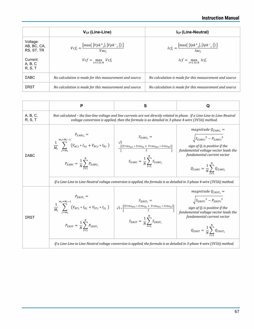
Instruction Manual
67
VCF (Line-Line) ICF (Line-Neutral)
Voltage: AB, BC, CA, RS, ST, TR
Current: A, B, C R, S, T
𝑉𝑉𝐸𝐸𝑉𝑉𝑖𝑖 =�max� �𝑉𝑉𝑐𝑐𝑉𝑉+𝑖𝑖�, �𝑉𝑉𝑐𝑐𝑉𝑉
−𝑖𝑖 �� �
𝑉𝑉𝐸𝐸𝐸𝐸𝑖𝑖
𝑉𝑉𝐸𝐸𝑉𝑉 = max𝑖𝑖=1 𝑡𝑡𝑡𝑡 𝑁𝑁
𝑉𝑉𝐸𝐸𝑉𝑉𝑖𝑖
𝐼𝐼𝐸𝐸𝑉𝑉𝑖𝑖 =�max� �𝐼𝐼𝑐𝑐𝑉𝑉+𝑖𝑖�, �𝐼𝐼𝑐𝑐𝑉𝑉
−𝑖𝑖 �� �
𝐼𝐼𝐸𝐸𝐸𝐸𝑖𝑖
𝐼𝐼𝐸𝐸𝑉𝑉 = max𝑖𝑖=1 𝑡𝑡𝑡𝑡 𝑁𝑁
𝐼𝐼𝐸𝐸𝑉𝑉𝑖𝑖
ΣABC No calculation is made for this measurement and source No calculation is made for this measurement and source
ΣRST No calculation is made for this measurement and source No calculation is made for this measurement and source
P S Q
A, B, C, R, S, T
Not calculated – the line-line voltage and line currents are not directly related in phase. If a Line-Line to Line-Neutral voltage conversion is applied, then the formula is as detailed in 3-phase 4-wire (3V3A) method.
ΣABC
𝑃𝑃𝛴𝛴𝛴𝛴𝛴𝛴𝛴𝛴𝑖𝑖 =
1𝑀𝑀𝑖𝑖
� �𝑉𝑉𝛴𝛴𝛴𝛴𝑗𝑗 ∗ 𝐼𝐼𝛴𝛴𝑗𝑗 + 𝑉𝑉𝛴𝛴𝛴𝛴𝑗𝑗 ∗ 𝐼𝐼𝛴𝛴𝑗𝑗 �𝑚𝑚𝑖𝑖+𝑀𝑀𝑖𝑖−1
𝑗𝑗=𝑚𝑚𝑖𝑖
𝑃𝑃𝛴𝛴𝛴𝛴𝛴𝛴𝛴𝛴 = 1𝑁𝑁�𝑃𝑃𝛴𝛴𝛴𝛴𝛴𝛴𝛴𝛴𝑖𝑖
𝑁𝑁
𝑖𝑖=1
𝑆𝑆𝛴𝛴𝛴𝛴𝛴𝛴𝛴𝛴𝑖𝑖 = √3
∗ �(𝑉𝑉𝑎𝑎𝑎𝑎𝑉𝑉𝛴𝛴𝛴𝛴𝑖𝑖 ∗ 𝐼𝐼𝑎𝑎𝑎𝑎𝑉𝑉𝛴𝛴𝑖𝑖 + 𝑉𝑉𝑎𝑎𝑎𝑎𝑉𝑉𝛴𝛴𝛴𝛴𝑖𝑖 ∗ 𝐼𝐼𝑎𝑎𝑎𝑎𝑉𝑉𝛴𝛴𝑖𝑖)
2�
𝑆𝑆𝛴𝛴𝛴𝛴𝛴𝛴𝛴𝛴 = 1𝑁𝑁�𝑆𝑆𝛴𝛴𝛴𝛴𝛴𝛴𝛴𝛴𝑖𝑖
𝑁𝑁
𝑖𝑖=1
𝑎𝑎𝐸𝐸𝑚𝑚𝑎𝑎𝑎𝑎𝐹𝐹𝐹𝐹𝑜𝑜𝑜𝑜 𝑄𝑄𝛴𝛴𝛴𝛴𝛴𝛴𝛴𝛴𝑖𝑖 =
�𝑆𝑆𝛴𝛴𝛴𝛴𝛴𝛴𝛴𝛴𝑖𝑖2 − 𝑃𝑃𝛴𝛴𝛴𝛴𝛴𝛴𝛴𝛴𝑖𝑖2
sign of Qi is positive if the fundamental voltage vector leads the
fundamental current vector
𝑄𝑄𝛴𝛴𝛴𝛴𝛴𝛴𝛴𝛴 = 1𝑁𝑁�𝑄𝑄𝛴𝛴𝛴𝛴𝛴𝛴𝛴𝛴𝑖𝑖
𝑁𝑁
𝑖𝑖=1
If a Line-Line to Line-Neutral voltage conversion is applied, the formula is as detailed in 3-phase 4-wire (3V3A) method.
ΣRST
𝑃𝑃𝛴𝛴𝛴𝛴𝛴𝛴𝛴𝛴𝑖𝑖 =
1𝑀𝑀𝑖𝑖
� �𝑉𝑉𝛴𝛴𝛴𝛴𝑗𝑗 ∗ 𝐼𝐼𝛴𝛴𝑗𝑗 + 𝑉𝑉𝛴𝛴𝛴𝛴𝑗𝑗 ∗ 𝐼𝐼𝛴𝛴𝑗𝑗 �𝑚𝑚𝑖𝑖+𝑀𝑀𝑖𝑖−1
𝑗𝑗=𝑚𝑚𝑖𝑖
𝑃𝑃𝛴𝛴𝛴𝛴𝛴𝛴𝛴𝛴 = 1𝑁𝑁�𝑃𝑃𝛴𝛴𝛴𝛴𝛴𝛴𝛴𝛴𝑖𝑖
𝑁𝑁
𝑖𝑖=1
𝑆𝑆𝛴𝛴𝛴𝛴𝛴𝛴𝛴𝛴𝑖𝑖 =
√3 ∗ �(𝑉𝑉𝑎𝑎𝑎𝑎𝑉𝑉𝛴𝛴𝛴𝛴𝑖𝑖 ∗ 𝐼𝐼𝑎𝑎𝑎𝑎𝑉𝑉𝛴𝛴𝑖𝑖 + 𝑉𝑉𝑎𝑎𝑎𝑎𝑉𝑉𝛴𝛴𝛴𝛴𝑖𝑖 ∗ 𝐼𝐼𝑎𝑎𝑎𝑎𝑉𝑉𝛴𝛴𝑖𝑖)
2�
𝑆𝑆𝛴𝛴𝛴𝛴𝛴𝛴𝛴𝛴 = 1𝑁𝑁�𝑆𝑆𝛴𝛴𝛴𝛴𝛴𝛴𝛴𝛴𝑖𝑖
𝑁𝑁
𝑖𝑖=1
𝑎𝑎𝐸𝐸𝑚𝑚𝑎𝑎𝑎𝑎𝐹𝐹𝐹𝐹𝑜𝑜𝑜𝑜 𝑄𝑄𝛴𝛴𝛴𝛴𝛴𝛴𝛴𝛴𝑖𝑖 =
�𝑆𝑆𝛴𝛴𝛴𝛴𝛴𝛴𝛴𝛴𝑖𝑖2 − 𝑃𝑃𝛴𝛴𝛴𝛴𝛴𝛴𝛴𝛴𝑖𝑖2
sign of Qi is positive if the fundamental voltage vector leads the
fundamental current vector
𝑄𝑄𝛴𝛴𝛴𝛴𝛴𝛴𝛴𝛴 = 1𝑁𝑁�𝑄𝑄𝛴𝛴𝛴𝛴𝛴𝛴𝛴𝛴𝑖𝑖
𝑁𝑁
𝑖𝑖=1
If a Line-Line to Line-Neutral voltage conversion is applied, the formula is as detailed in 3-phase 4-wire (3V3A) method.

3-phase Power Analysis Software
68
PPK+, PPK- λ (Power Factor) ϕ (Phase Angle)
A, B, C, R, S, T
Not calculated – the line-line voltage and line currents are not directly related in phase. If a Line-Line to Line-Neutral voltage conversion is applied, the formula is as detailed in 3-phase 4-wire (3V3A) method.
ΣABC
𝑃𝑃𝑐𝑐𝑉𝑉+𝛴𝛴𝛴𝛴𝛴𝛴𝛴𝛴𝑖𝑖 =
max𝑗𝑗=𝑚𝑚𝑖𝑖 𝑡𝑡𝑡𝑡 𝑚𝑚𝑖𝑖+𝑀𝑀𝑖𝑖−1
�𝑉𝑉𝛴𝛴𝛴𝛴𝑗𝑗 ∗ 𝐼𝐼𝛴𝛴𝑗𝑗 + 𝑉𝑉𝛴𝛴𝛴𝛴𝑗𝑗 ∗ 𝐼𝐼𝛴𝛴𝑗𝑗�
𝑃𝑃𝑐𝑐𝑉𝑉⁻𝛴𝛴𝛴𝛴𝛴𝛴𝛴𝛴𝑖𝑖 =
min𝑗𝑗=𝑚𝑚𝑖𝑖 𝑡𝑡𝑡𝑡 𝑚𝑚𝑖𝑖+𝑀𝑀𝑖𝑖−1
�𝑉𝑉𝛴𝛴𝛴𝛴𝑗𝑗 ∗ 𝐼𝐼𝛴𝛴𝑗𝑗 + 𝑉𝑉𝛴𝛴𝛴𝛴𝑗𝑗 ∗ 𝐼𝐼𝛴𝛴𝑗𝑗�
𝑃𝑃𝑐𝑐𝑉𝑉+𝛴𝛴𝛴𝛴𝛴𝛴𝛴𝛴 = max𝑖𝑖=1 𝑡𝑡𝑡𝑡 𝑁𝑁
𝑃𝑃𝑐𝑐𝑉𝑉+𝛴𝛴𝛴𝛴𝛴𝛴𝛴𝛴𝑖𝑖
𝑃𝑃𝑐𝑐𝑉𝑉⁻𝛴𝛴𝛴𝛴𝛴𝛴𝛴𝛴 = min𝑖𝑖=1 𝑡𝑡𝑡𝑡 𝑁𝑁
𝑃𝑃𝑐𝑐𝑉𝑉⁻𝛴𝛴𝛴𝛴𝛴𝛴𝛴𝛴𝑖𝑖
𝜆𝜆𝛴𝛴𝛴𝛴𝛴𝛴𝛴𝛴𝑖𝑖 = 𝑃𝑃𝛴𝛴𝛴𝛴𝛴𝛴𝛴𝛴𝑖𝑖 𝑆𝑆𝛴𝛴𝛴𝛴𝛴𝛴𝛴𝛴𝑖𝑖�
𝜆𝜆𝛴𝛴𝛴𝛴𝛴𝛴𝛴𝛴 = 1𝑁𝑁�
𝑃𝑃𝛴𝛴𝛴𝛴𝛴𝛴𝛴𝛴𝑖𝑖𝑆𝑆𝛴𝛴𝛴𝛴𝛴𝛴𝛴𝛴𝑖𝑖�
𝑁𝑁
𝑖𝑖=1
𝑎𝑎𝐸𝐸𝑚𝑚𝑎𝑎𝑎𝑎𝐹𝐹𝐹𝐹𝑜𝑜𝑜𝑜 𝜙𝜙𝛴𝛴𝛴𝛴𝛴𝛴𝛴𝛴𝑖𝑖 = cos−1 𝜆𝜆𝛴𝛴𝛴𝛴𝛴𝛴𝛴𝛴𝑖𝑖 sign of ϕi is positive if the fundamental voltage vector leads the fundamental
current vector
𝜙𝜙𝛴𝛴𝛴𝛴𝛴𝛴𝛴𝛴 = 1𝑁𝑁� cos−1 𝜆𝜆𝛴𝛴𝛴𝛴𝛴𝛴𝛴𝛴𝑖𝑖
𝑁𝑁
𝑖𝑖=1
If a Line-Line to Line-Neutral voltage conversion is applied, the formula is as detailed in 3-phase 4-wire (3V3A) method.
ΣRST
𝑃𝑃𝑐𝑐𝑉𝑉+𝛴𝛴𝛴𝛴𝛴𝛴𝛴𝛴𝑖𝑖 =
max𝑗𝑗=𝑚𝑚𝑖𝑖 𝑡𝑡𝑡𝑡 𝑚𝑚𝑖𝑖+𝑀𝑀𝑖𝑖−1
�𝑉𝑉𝛴𝛴𝛴𝛴𝑗𝑗 ∗ 𝐼𝐼𝛴𝛴𝑗𝑗 + 𝑉𝑉𝛴𝛴𝛴𝛴𝑗𝑗 ∗ 𝐼𝐼𝛴𝛴𝑗𝑗�
𝑃𝑃𝑐𝑐𝑉𝑉⁻𝛴𝛴𝛴𝛴𝛴𝛴𝛴𝛴𝑖𝑖 =
min𝑗𝑗=𝑚𝑚𝑖𝑖 𝑡𝑡𝑡𝑡 𝑚𝑚𝑖𝑖+𝑀𝑀𝑖𝑖−1
�𝑉𝑉𝛴𝛴𝛴𝛴𝑗𝑗 ∗ 𝐼𝐼𝛴𝛴𝑗𝑗 + 𝑉𝑉𝛴𝛴𝛴𝛴𝑗𝑗 ∗ 𝐼𝐼𝛴𝛴𝑗𝑗�
𝑃𝑃𝑐𝑐𝑉𝑉+𝛴𝛴𝛴𝛴𝛴𝛴𝛴𝛴 = max𝑖𝑖=1 𝑡𝑡𝑡𝑡 𝑁𝑁
𝑃𝑃𝑐𝑐𝑉𝑉+𝛴𝛴𝛴𝛴𝛴𝛴𝛴𝛴𝑖𝑖
𝑃𝑃𝑐𝑐𝑉𝑉⁻𝛴𝛴𝛴𝛴𝛴𝛴𝛴𝛴 = min𝑖𝑖=1 𝑡𝑡𝑡𝑡 𝑁𝑁
𝑃𝑃𝑐𝑐𝑉𝑉⁻𝛴𝛴𝛴𝛴𝛴𝛴𝛴𝛴𝑖𝑖
𝜆𝜆𝛴𝛴𝛴𝛴𝛴𝛴𝛴𝛴𝑖𝑖 = 𝑃𝑃𝛴𝛴𝛴𝛴𝛴𝛴𝛴𝛴𝑖𝑖 𝑆𝑆𝛴𝛴𝛴𝛴𝛴𝛴𝛴𝛴𝑖𝑖�
𝜆𝜆𝛴𝛴𝛴𝛴𝛴𝛴𝛴𝛴 = 1𝑁𝑁�
𝑃𝑃𝛴𝛴𝛴𝛴𝛴𝛴𝛴𝛴𝑖𝑖𝑆𝑆𝛴𝛴𝛴𝛴𝛴𝛴𝛴𝛴𝑖𝑖�
𝑁𝑁
𝑖𝑖=1
𝑎𝑎𝐸𝐸𝑚𝑚𝑎𝑎𝑎𝑎𝐹𝐹𝐹𝐹𝑜𝑜𝑜𝑜 𝜙𝜙𝛴𝛴𝛴𝛴𝛴𝛴𝛴𝛴𝑖𝑖 = cos−1 𝜆𝜆𝛴𝛴𝛴𝛴𝛴𝛴𝛴𝛴𝑖𝑖 sign of ϕi is positive if the fundamental voltage vector leads the fundamental
current vector
𝜙𝜙𝛴𝛴𝛴𝛴𝛴𝛴𝛴𝛴 = 1𝑁𝑁� cos−1 𝜆𝜆𝛴𝛴𝛴𝛴𝛴𝛴𝛴𝛴𝑖𝑖
𝑁𝑁
𝑖𝑖=1
If a Line-Line to Line-Neutral voltage conversion is applied, the formula is as detailed in 3-phase 4-wire (3V3A) method.
Slip Stage-Stage Efficiency (η1) Cumulative Efficiency (η2)
ΣABC DC Bus ΣRST
𝑆𝑆𝐹𝐹𝑎𝑎𝑐𝑐𝑖𝑖 = 1𝑀𝑀𝑖𝑖
� �𝜔𝜔𝑉𝑉𝑗𝑗 − 𝜔𝜔𝑗𝑗
𝜔𝜔𝑗𝑗�
𝑚𝑚𝑖𝑖+𝑀𝑀𝑖𝑖−1
𝑗𝑗=𝑚𝑚𝑖𝑖
ωsj is the instantaneous speed calculation of the stator magnetic
field. ωsj and ωj are calculated internally and are not displayed.
𝑆𝑆𝐹𝐹𝑎𝑎𝑐𝑐 = 1𝑁𝑁�𝑆𝑆𝐹𝐹𝑎𝑎𝑐𝑐𝑖𝑖
𝑁𝑁
𝑖𝑖=1
𝜂𝜂1𝑖𝑖 = �𝑃𝑃𝛴𝛴𝛴𝛴𝛴𝛴𝑆𝑆𝑆𝑆2𝑖𝑖𝑃𝑃𝛴𝛴𝛴𝛴𝛴𝛴𝑆𝑆𝑆𝑆1𝑖𝑖
� ∗ 100%
𝑁𝑁𝐹𝐹𝑎𝑎𝑜𝑜𝑎𝑎𝑎𝑎𝐸𝐸 𝐹𝐹𝐸𝐸𝑡𝑡𝐹𝐹𝑜𝑜 𝑣𝑣𝐸𝐸𝐹𝐹𝐹𝐹𝑜𝑜𝑉𝑉1𝑁𝑁�𝜂𝜂1𝑖𝑖
𝑁𝑁
𝑖𝑖=1
In the event of unequal sync cycle periods, a new efficiency value will
be calculated on each cyclic positive transition.
𝜂𝜂2𝑖𝑖 = �𝑃𝑃𝐿𝐿𝛴𝛴𝛴𝛴𝛴𝛴𝑖𝑖𝑃𝑃𝐹𝐹𝐹𝐹𝛴𝛴𝛴𝛴𝛴𝛴𝑖𝑖
� ∗ 100%
𝑁𝑁𝐹𝐹𝑎𝑎𝑜𝑜𝑎𝑎𝑎𝑎𝐸𝐸 𝐹𝐹𝐸𝐸𝑡𝑡𝐹𝐹𝑜𝑜 𝑣𝑣𝐸𝐸𝐹𝐹𝐹𝐹𝑜𝑜𝑉𝑉1𝑁𝑁�𝜂𝜂2𝑖𝑖
𝑁𝑁
𝑖𝑖=1
In the event of unequal sync cycle periods, a new efficiency value will be
calculated on each cyclic positive transition.
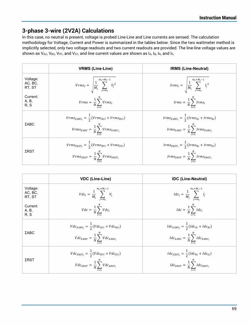
Instruction Manual
69
3-phase 3-wire (2V2A) Calculations In this case, no neutral is present, voltage is probed Line-Line and Line currents are sensed. The calculation methodology for Voltage, Current and Power is summarized in the tables below. Since the two wattmeter method is implicitly selected, only two voltage readouts and two current readouts are provided. The line-line voltage values are shown as VAC, VBC, VRT, and VST, and line current values are shown as IA, IB, IR, and IS.
VRMS (Line-Line) IRMS (Line-Neutral)
Voltage: AC, BC, RT, ST
Current: A, B, R, S
𝑉𝑉𝑎𝑎𝑎𝑎𝑉𝑉𝑖𝑖 = �1𝑀𝑀𝑖𝑖
� 𝑉𝑉𝑗𝑗2𝑚𝑚𝑖𝑖+𝑀𝑀𝑖𝑖−1
𝑗𝑗=𝑚𝑚𝑖𝑖
𝑉𝑉𝑎𝑎𝑎𝑎𝑉𝑉 = 1𝑁𝑁�𝑉𝑉𝑎𝑎𝑎𝑎𝑉𝑉𝑖𝑖
𝑁𝑁
𝑖𝑖=1
𝐼𝐼𝑎𝑎𝑎𝑎𝑉𝑉𝑖𝑖 = �1𝑀𝑀𝑖𝑖
� 𝐼𝐼𝑗𝑗2𝑚𝑚𝑖𝑖+𝑀𝑀𝑖𝑖−1
𝑗𝑗=𝑚𝑚𝑖𝑖
𝐼𝐼𝑎𝑎𝑎𝑎𝑉𝑉 = 1𝑁𝑁�𝐼𝐼𝑎𝑎𝑎𝑎𝑉𝑉𝑖𝑖
𝑁𝑁
𝑖𝑖=1
ΣABC
𝑉𝑉𝑎𝑎𝑎𝑎𝑉𝑉𝛴𝛴𝛴𝛴𝛴𝛴𝛴𝛴𝑖𝑖 = 12
(𝑉𝑉𝑎𝑎𝑎𝑎𝑉𝑉𝛴𝛴𝛴𝛴𝑖𝑖 + 𝑉𝑉𝑎𝑎𝑎𝑎𝑉𝑉𝛴𝛴𝛴𝛴𝑖𝑖)
𝑉𝑉𝑎𝑎𝑎𝑎𝑉𝑉𝛴𝛴𝛴𝛴𝛴𝛴𝛴𝛴 = 1𝑁𝑁�𝑉𝑉𝑎𝑎𝑎𝑎𝑉𝑉𝛴𝛴𝛴𝛴𝛴𝛴𝛴𝛴𝑖𝑖
𝑁𝑁
𝑖𝑖=1
𝐼𝐼𝑎𝑎𝑎𝑎𝑉𝑉𝛴𝛴𝛴𝛴𝛴𝛴𝛴𝛴𝑖𝑖 = 12
(𝐼𝐼𝑎𝑎𝑎𝑎𝑉𝑉𝛴𝛴𝑖𝑖 + 𝐼𝐼𝑎𝑎𝑎𝑎𝑉𝑉𝛴𝛴𝑖𝑖)
𝐼𝐼𝑎𝑎𝑎𝑎𝑉𝑉𝛴𝛴𝛴𝛴𝛴𝛴𝛴𝛴 = 1𝑁𝑁�𝐼𝐼𝑎𝑎𝑎𝑎𝑉𝑉𝛴𝛴𝛴𝛴𝛴𝛴𝛴𝛴𝑖𝑖
𝑁𝑁
𝑖𝑖=1
ΣRST
𝑉𝑉𝑎𝑎𝑎𝑎𝑉𝑉𝛴𝛴𝛴𝛴𝛴𝛴𝛴𝛴𝑖𝑖 = 12
(𝑉𝑉𝑎𝑎𝑎𝑎𝑉𝑉𝛴𝛴𝛴𝛴𝑖𝑖 + 𝑉𝑉𝑎𝑎𝑎𝑎𝑉𝑉𝛴𝛴𝛴𝛴𝑖𝑖)
𝑉𝑉𝑎𝑎𝑎𝑎𝑉𝑉𝛴𝛴𝛴𝛴𝛴𝛴𝛴𝛴 = 1𝑁𝑁�𝑉𝑉𝑎𝑎𝑎𝑎𝑉𝑉𝛴𝛴𝛴𝛴𝛴𝛴𝛴𝛴𝑖𝑖
𝑁𝑁
𝑖𝑖=1
𝐼𝐼𝑎𝑎𝑎𝑎𝑉𝑉𝛴𝛴𝛴𝛴𝛴𝛴𝛴𝛴𝑖𝑖 = 12
(𝐼𝐼𝑎𝑎𝑎𝑎𝑉𝑉𝛴𝛴𝑖𝑖 + 𝐼𝐼𝑎𝑎𝑎𝑎𝑉𝑉𝛴𝛴𝑖𝑖)
𝐼𝐼𝑎𝑎𝑎𝑎𝑉𝑉𝛴𝛴𝛴𝛴𝛴𝛴𝛴𝛴 = 1𝑁𝑁�𝐼𝐼𝑎𝑎𝑎𝑎𝑉𝑉𝛴𝛴𝛴𝛴𝛴𝛴𝛴𝛴𝑖𝑖
𝑁𝑁
𝑖𝑖=1
VDC (Line-Line) IDC (Line-Neutral)
Voltage: AC, BC, RT, ST
Current: A, B, R, S
𝑉𝑉𝑜𝑜𝐸𝐸𝑖𝑖 = 1𝑀𝑀𝑖𝑖
� 𝑉𝑉𝑗𝑗
𝑚𝑚𝑖𝑖+𝑀𝑀𝑖𝑖−1
𝑗𝑗=𝑚𝑚𝑖𝑖
𝑉𝑉𝑜𝑜𝐸𝐸 = 1𝑁𝑁�𝑉𝑉𝑜𝑜𝐸𝐸𝑖𝑖
𝑁𝑁
𝑖𝑖=1
𝐼𝐼𝑜𝑜𝐸𝐸𝑖𝑖 = 1𝑀𝑀𝑖𝑖
� 𝐼𝐼𝑗𝑗
𝑚𝑚𝑖𝑖+𝑀𝑀𝑖𝑖−1
𝑗𝑗=𝑚𝑚𝑖𝑖
𝐼𝐼𝑜𝑜𝐸𝐸 = 1𝑁𝑁�𝐼𝐼𝑜𝑜𝐸𝐸𝑖𝑖
𝑁𝑁
𝑖𝑖=1
ΣABC
𝑉𝑉𝑜𝑜𝐸𝐸𝛴𝛴𝛴𝛴𝛴𝛴𝛴𝛴𝑖𝑖 = 12
(𝑉𝑉𝑜𝑜𝐸𝐸𝛴𝛴𝛴𝛴𝑖𝑖 + 𝑉𝑉𝑜𝑜𝐸𝐸𝛴𝛴𝛴𝛴𝑖𝑖)
𝑉𝑉𝑜𝑜𝐸𝐸𝛴𝛴𝛴𝛴𝛴𝛴𝛴𝛴 = 1𝑁𝑁�𝑉𝑉𝑜𝑜𝐸𝐸𝛴𝛴𝛴𝛴𝛴𝛴𝛴𝛴𝑖𝑖
𝑁𝑁
𝑖𝑖=1
𝐼𝐼𝑜𝑜𝐸𝐸𝛴𝛴𝛴𝛴𝛴𝛴𝛴𝛴𝑖𝑖 = 12
(𝐼𝐼𝑜𝑜𝐸𝐸𝛴𝛴𝑖𝑖 + 𝐼𝐼𝑜𝑜𝐸𝐸𝛴𝛴𝑖𝑖)
𝐼𝐼𝑜𝑜𝐸𝐸𝛴𝛴𝛴𝛴𝛴𝛴𝛴𝛴 = 1𝑁𝑁�𝐼𝐼𝑜𝑜𝐸𝐸𝛴𝛴𝛴𝛴𝛴𝛴𝛴𝛴𝑖𝑖
𝑁𝑁
𝑖𝑖=1
ΣRST
𝑉𝑉𝑜𝑜𝐸𝐸𝛴𝛴𝛴𝛴𝛴𝛴𝛴𝛴𝑖𝑖 = 12
(𝑉𝑉𝑜𝑜𝐸𝐸𝛴𝛴𝛴𝛴𝑖𝑖 + 𝑉𝑉𝑜𝑜𝐸𝐸𝛴𝛴𝛴𝛴𝑖𝑖)
𝑉𝑉𝑜𝑜𝐸𝐸𝛴𝛴𝛴𝛴𝛴𝛴𝛴𝛴 = 1𝑁𝑁�𝑉𝑉𝑜𝑜𝐸𝐸𝛴𝛴𝛴𝛴𝛴𝛴𝛴𝛴𝑖𝑖
𝑁𝑁
𝑖𝑖=1
𝐼𝐼𝑜𝑜𝐸𝐸𝛴𝛴𝛴𝛴𝛴𝛴𝛴𝛴𝑖𝑖 = 12
(𝐼𝐼𝑜𝑜𝐸𝐸𝛴𝛴𝑖𝑖 + 𝐼𝐼𝑜𝑜𝐸𝐸𝛴𝛴𝑖𝑖)
𝐼𝐼𝑜𝑜𝐸𝐸𝛴𝛴𝛴𝛴𝛴𝛴𝛴𝛴 = 1𝑁𝑁�𝐼𝐼𝑜𝑜𝐸𝐸𝛴𝛴𝛴𝛴𝛴𝛴𝛴𝛴𝑖𝑖
𝑁𝑁
𝑖𝑖=1

3-phase Power Analysis Software
70
VAC (Line-Line) IAC (Line-Neutral)
Voltage: AC, BC, RT, ST
Current: A, B, R, S
𝑉𝑉𝐸𝐸𝐸𝐸𝑖𝑖 = 𝑉𝑉𝑎𝑎𝑎𝑎𝑉𝑉𝑖𝑖 − 𝑉𝑉𝑜𝑜𝐸𝐸𝑖𝑖
𝑉𝑉𝐸𝐸𝐸𝐸 = 1𝑁𝑁�𝑉𝑉𝐸𝐸𝐸𝐸𝑖𝑖
𝑁𝑁
𝑖𝑖=1
𝐼𝐼𝐸𝐸𝐸𝐸𝑖𝑖 = 𝐼𝐼𝑎𝑎𝑎𝑎𝑉𝑉𝑖𝑖 − 𝐼𝐼𝑜𝑜𝐸𝐸𝑖𝑖
𝐼𝐼𝐸𝐸𝐸𝐸 = 1𝑁𝑁�𝐼𝐼𝐸𝐸𝐸𝐸𝑖𝑖
𝑁𝑁
𝑖𝑖=1
ΣABC
𝑉𝑉𝐸𝐸𝐸𝐸𝛴𝛴𝛴𝛴𝛴𝛴𝛴𝛴𝑖𝑖 = 12
(𝑉𝑉𝐸𝐸𝐸𝐸𝛴𝛴𝛴𝛴𝑖𝑖 + 𝑉𝑉𝐸𝐸𝐸𝐸𝛴𝛴𝛴𝛴𝑖𝑖)
𝑉𝑉𝐸𝐸𝐸𝐸𝛴𝛴𝛴𝛴𝛴𝛴𝛴𝛴 = 1𝑁𝑁�𝑉𝑉𝐸𝐸𝐸𝐸𝛴𝛴𝛴𝛴𝛴𝛴𝛴𝛴𝑖𝑖
𝑁𝑁
𝑖𝑖=1
𝐼𝐼𝐸𝐸𝐸𝐸𝛴𝛴𝛴𝛴𝛴𝛴𝛴𝛴𝑖𝑖 = 12
(𝐼𝐼𝐸𝐸𝐸𝐸𝛴𝛴𝑖𝑖 + 𝐼𝐼𝐸𝐸𝐸𝐸𝛴𝛴𝑖𝑖)
𝐼𝐼𝐸𝐸𝐸𝐸𝛴𝛴𝛴𝛴𝛴𝛴𝛴𝛴 = 1𝑁𝑁�𝐼𝐼𝐸𝐸𝐸𝐸𝛴𝛴𝛴𝛴𝛴𝛴𝛴𝛴𝑖𝑖
𝑁𝑁
𝑖𝑖=1
ΣRST
𝑉𝑉𝐸𝐸𝐸𝐸𝛴𝛴𝛴𝛴𝛴𝛴𝛴𝛴𝑖𝑖 = 12
(𝑉𝑉𝐸𝐸𝐸𝐸𝛴𝛴𝛴𝛴𝑖𝑖 + 𝑉𝑉𝐸𝐸𝐸𝐸𝛴𝛴𝛴𝛴𝑖𝑖)
𝑉𝑉𝐸𝐸𝐸𝐸𝛴𝛴𝛴𝛴𝛴𝛴𝛴𝛴 = 1𝑁𝑁�𝑉𝑉𝐸𝐸𝐸𝐸𝛴𝛴𝛴𝛴𝛴𝛴𝛴𝛴𝑖𝑖
𝑁𝑁
𝑖𝑖=1
𝐼𝐼𝐸𝐸𝐸𝐸𝛴𝛴𝛴𝛴𝛴𝛴𝛴𝛴𝑖𝑖 = 12
(𝐼𝐼𝐸𝐸𝐸𝐸𝛴𝛴𝑖𝑖 + 𝐼𝐼𝐸𝐸𝐸𝐸𝛴𝛴𝑖𝑖)
𝐼𝐼𝐸𝐸𝐸𝐸𝛴𝛴𝛴𝛴𝛴𝛴𝛴𝛴 = 1𝑁𝑁�𝐼𝐼𝐸𝐸𝐸𝐸𝛴𝛴𝛴𝛴𝛴𝛴𝛴𝛴𝑖𝑖
𝑁𝑁
𝑖𝑖=1
VPK+, VPK-, VPK-PK (Line-Line) IPK+, IPK-, IPK-PK (Line-Neutral)
Voltage: AC, BC, RT, ST
Current: A, B, R, S
𝑉𝑉𝑐𝑐𝑉𝑉⁺𝑖𝑖 = max𝑗𝑗=𝑚𝑚𝑖𝑖 𝑡𝑡𝑡𝑡 𝑚𝑚𝑖𝑖+𝑀𝑀𝑖𝑖−1
𝑉𝑉𝑗𝑗
𝑉𝑉𝑐𝑐𝑉𝑉⁻𝑖𝑖 = min𝑗𝑗=𝑚𝑚𝑖𝑖 𝑡𝑡𝑡𝑡 𝑚𝑚𝑖𝑖+𝑀𝑀𝑖𝑖−1
𝑉𝑉𝑗𝑗
𝑉𝑉𝑐𝑐𝑉𝑉⎼𝑐𝑐𝑉𝑉𝑖𝑖 = 𝑉𝑉𝑐𝑐𝑉𝑉⁺𝑖𝑖 − 𝑉𝑉𝑐𝑐𝑉𝑉⁻𝑖𝑖
𝑉𝑉𝑐𝑐𝑉𝑉+ = max𝑖𝑖=1 𝑡𝑡𝑡𝑡 𝑁𝑁
𝑉𝑉𝑐𝑐𝑉𝑉⁺𝑖𝑖
𝑉𝑉𝑐𝑐𝑉𝑉⁻ = min𝑖𝑖=1 𝑡𝑡𝑡𝑡 𝑁𝑁
𝑉𝑉𝑐𝑐𝑉𝑉⁻𝑖𝑖
𝑉𝑉𝑐𝑐𝑉𝑉⎼𝑐𝑐𝑉𝑉 = max𝑖𝑖=1 𝑡𝑡𝑡𝑡 𝑁𝑁
𝑉𝑉𝑐𝑐𝑉𝑉⎼𝑐𝑐𝑉𝑉𝑖𝑖
𝐼𝐼𝑐𝑐𝑉𝑉⁺𝑖𝑖 = max𝑗𝑗=𝑚𝑚𝑖𝑖 𝑡𝑡𝑡𝑡 𝑚𝑚𝑖𝑖+𝑀𝑀𝑖𝑖−1
𝐼𝐼𝑗𝑗
𝐼𝐼𝑐𝑐𝑉𝑉⁻𝑖𝑖 = min𝑗𝑗=𝑚𝑚𝑖𝑖 𝑡𝑡𝑡𝑡 𝑚𝑚𝑖𝑖+𝑀𝑀𝑖𝑖−1
𝐼𝐼𝑗𝑗
𝐼𝐼𝑐𝑐𝑉𝑉⎼𝑐𝑐𝑉𝑉𝑖𝑖 = 𝐼𝐼𝑐𝑐𝑉𝑉⁺𝑖𝑖 − 𝐼𝐼𝑐𝑐𝑉𝑉⁻𝑖𝑖
𝐼𝐼𝑐𝑐𝑉𝑉+ = max𝑖𝑖=1 𝑡𝑡𝑡𝑡 𝑁𝑁
𝐼𝐼𝑐𝑐𝑉𝑉⁺𝑖𝑖
𝐼𝐼𝑐𝑐𝑉𝑉⁻ = max𝑖𝑖=1 𝑡𝑡𝑡𝑡 𝑁𝑁
𝐼𝐼𝑐𝑐𝑉𝑉⁻𝑖𝑖
𝐼𝐼𝑐𝑐𝑉𝑉⎼𝑐𝑐𝑉𝑉 = max𝑖𝑖=1 𝑡𝑡𝑡𝑡 𝑁𝑁
𝐼𝐼𝑐𝑐𝑉𝑉⎼𝑐𝑐𝑉𝑉𝑖𝑖
ΣABC
𝑉𝑉𝑐𝑐𝑉𝑉+𝛴𝛴𝛴𝛴𝛴𝛴𝛴𝛴𝑖𝑖 = max�𝑉𝑉𝑐𝑐𝑉𝑉+𝛴𝛴𝛴𝛴𝑖𝑖 ,𝑉𝑉𝑐𝑐𝑉𝑉+𝛴𝛴𝛴𝛴𝑖𝑖�
𝑉𝑉𝑐𝑐𝑉𝑉⁻𝛴𝛴𝛴𝛴𝛴𝛴𝛴𝛴𝑖𝑖 = max�𝑉𝑉𝑐𝑐𝑉𝑉⁻𝛴𝛴𝛴𝛴𝑖𝑖 ,𝑉𝑉𝑐𝑐𝑉𝑉⁻𝛴𝛴𝛴𝛴𝑖𝑖�
𝑉𝑉𝑐𝑐𝑉𝑉⎼𝑐𝑐𝑉𝑉𝛴𝛴𝛴𝛴𝛴𝛴𝛴𝛴𝑖𝑖 = max(𝑉𝑉𝑐𝑐𝑉𝑉⎼𝑐𝑐𝑉𝑉𝛴𝛴𝛴𝛴𝑖𝑖 ,𝑉𝑉𝑐𝑐𝑉𝑉⎼𝑐𝑐𝑉𝑉𝛴𝛴𝛴𝛴𝑖𝑖) 𝑉𝑉𝑐𝑐𝑉𝑉+𝛴𝛴𝛴𝛴𝛴𝛴𝛴𝛴 = max
𝑖𝑖=1 𝑡𝑡𝑡𝑡 𝑁𝑁 𝑉𝑉𝑐𝑐𝑉𝑉+𝛴𝛴𝛴𝛴𝛴𝛴𝛴𝛴𝑖𝑖
𝑉𝑉𝑐𝑐𝑉𝑉⁻𝛴𝛴𝛴𝛴𝛴𝛴𝛴𝛴 = min𝑖𝑖=1 𝑡𝑡𝑡𝑡 𝑁𝑁
𝑉𝑉𝑐𝑐𝑉𝑉⁻𝛴𝛴𝛴𝛴𝛴𝛴𝛴𝛴𝑖𝑖
𝑉𝑉𝑐𝑐𝑉𝑉⎼𝑐𝑐𝑉𝑉𝛴𝛴𝛴𝛴𝛴𝛴𝛴𝛴 = max𝑖𝑖=1 𝑡𝑡𝑡𝑡 𝑁𝑁
𝑉𝑉𝑐𝑐𝑉𝑉⎼𝑐𝑐𝑉𝑉𝛴𝛴𝛴𝛴𝛴𝛴𝛴𝛴𝑖𝑖
𝐼𝐼𝑐𝑐𝑉𝑉+𝛴𝛴𝛴𝛴𝛴𝛴𝛴𝛴𝑖𝑖 = max�𝐼𝐼𝑐𝑐𝑉𝑉+𝛴𝛴𝑖𝑖 , 𝐼𝐼𝑐𝑐𝑉𝑉+𝛴𝛴𝑖𝑖�
𝐼𝐼𝑐𝑐𝑉𝑉⁻𝛴𝛴𝛴𝛴𝛴𝛴𝛴𝛴𝑖𝑖 = min�𝐼𝐼𝑐𝑐𝑉𝑉⁻𝛴𝛴𝑖𝑖 , 𝐼𝐼𝑐𝑐𝑉𝑉⁻𝛴𝛴𝑖𝑖�
𝐼𝐼𝑐𝑐𝑉𝑉⎼𝑐𝑐𝑉𝑉𝛴𝛴𝛴𝛴𝛴𝛴𝛴𝛴𝑖𝑖 = max(𝐼𝐼𝑐𝑐𝑉𝑉⎼𝑐𝑐𝑉𝑉𝛴𝛴𝑖𝑖 , 𝐼𝐼𝑐𝑐𝑉𝑉⎼𝑐𝑐𝑉𝑉𝛴𝛴𝑖𝑖) 𝐼𝐼𝑐𝑐𝑉𝑉+𝛴𝛴𝛴𝛴𝛴𝛴𝛴𝛴 = max
𝑖𝑖=1 𝑡𝑡𝑡𝑡 𝑁𝑁 𝐼𝐼𝑐𝑐𝑉𝑉+𝛴𝛴𝛴𝛴𝛴𝛴𝛴𝛴𝑖𝑖
𝐼𝐼𝑐𝑐𝑉𝑉⁻𝛴𝛴𝛴𝛴𝛴𝛴𝛴𝛴 = min𝑖𝑖=1 𝑡𝑡𝑡𝑡 𝑁𝑁
𝐼𝐼𝑐𝑐𝑉𝑉⁻𝛴𝛴𝛴𝛴𝛴𝛴𝛴𝛴𝑖𝑖
𝐼𝐼𝑐𝑐𝑉𝑉⎼𝑐𝑐𝑉𝑉𝛴𝛴𝛴𝛴𝛴𝛴𝛴𝛴 = max𝑖𝑖=1 𝑡𝑡𝑡𝑡 𝑁𝑁
𝐼𝐼𝑐𝑐𝑉𝑉⎼𝑐𝑐𝑉𝑉𝛴𝛴𝛴𝛴𝛴𝛴𝛴𝛴𝑖𝑖
ΣRST
𝑉𝑉𝑐𝑐𝑉𝑉+𝛴𝛴𝛴𝛴𝛴𝛴𝛴𝛴𝑖𝑖 = max�𝑉𝑉𝑐𝑐𝑉𝑉+𝛴𝛴𝛴𝛴𝑖𝑖 ,𝑉𝑉𝑐𝑐𝑉𝑉+𝛴𝛴𝛴𝛴𝑖𝑖�
𝑉𝑉𝑐𝑐𝑉𝑉⁻𝛴𝛴𝛴𝛴𝛴𝛴𝛴𝛴𝑖𝑖 = min�𝑉𝑉𝑐𝑐𝑉𝑉⁻𝛴𝛴𝛴𝛴𝑖𝑖 ,𝑉𝑉𝑐𝑐𝑉𝑉⁻𝛴𝛴𝛴𝛴𝑖𝑖�
𝑉𝑉𝑐𝑐𝑉𝑉⎼𝑐𝑐𝑉𝑉𝛴𝛴𝛴𝛴𝛴𝛴𝛴𝛴𝑖𝑖 = max(𝑉𝑉𝑐𝑐𝑉𝑉⎼𝑐𝑐𝑉𝑉𝛴𝛴𝛴𝛴𝑖𝑖 ,𝑉𝑉𝑐𝑐𝑉𝑉⎼𝑐𝑐𝑉𝑉𝛴𝛴𝛴𝛴𝑖𝑖) 𝑉𝑉𝑐𝑐𝑉𝑉+𝛴𝛴𝛴𝛴𝛴𝛴𝛴𝛴 = max
𝑖𝑖=1 𝑡𝑡𝑡𝑡 𝑁𝑁 𝑉𝑉𝑐𝑐𝑉𝑉+𝛴𝛴𝛴𝛴𝛴𝛴𝛴𝛴𝑖𝑖
𝑉𝑉𝑐𝑐𝑉𝑉⁻𝛴𝛴𝛴𝛴𝛴𝛴𝛴𝛴 = min𝑖𝑖=1 𝑡𝑡𝑡𝑡 𝑁𝑁
𝑉𝑉𝑐𝑐𝑉𝑉⁻𝛴𝛴𝛴𝛴𝛴𝛴𝛴𝛴𝑖𝑖
𝑉𝑉𝑐𝑐𝑉𝑉⎼𝑐𝑐𝑉𝑉𝛴𝛴𝛴𝛴𝛴𝛴𝛴𝛴 = max𝑖𝑖=1 𝑡𝑡𝑡𝑡 𝑁𝑁
𝑉𝑉𝑐𝑐𝑉𝑉⎼𝑐𝑐𝑉𝑉𝛴𝛴𝛴𝛴𝛴𝛴𝛴𝛴𝑖𝑖
𝐼𝐼𝑐𝑐𝑉𝑉+𝛴𝛴𝛴𝛴𝛴𝛴𝛴𝛴𝑖𝑖 = max�𝐼𝐼𝑐𝑐𝑉𝑉+𝛴𝛴𝑖𝑖 , 𝐼𝐼𝑐𝑐𝑉𝑉+𝛴𝛴𝑖𝑖�
𝐼𝐼𝑐𝑐𝑉𝑉⁻𝛴𝛴𝛴𝛴𝛴𝛴𝛴𝛴𝑖𝑖 = min�𝐼𝐼𝑐𝑐𝑉𝑉⁻𝛴𝛴𝑖𝑖 , 𝐼𝐼𝑐𝑐𝑉𝑉⁻𝛴𝛴𝑖𝑖�
𝐼𝐼𝑐𝑐𝑉𝑉⎼𝑐𝑐𝑉𝑉𝛴𝛴𝛴𝛴𝛴𝛴𝛴𝛴𝑖𝑖 = max(𝐼𝐼𝑐𝑐𝑉𝑉⎼𝑐𝑐𝑉𝑉𝛴𝛴𝑖𝑖 , 𝐼𝐼𝑐𝑐𝑉𝑉⎼𝑐𝑐𝑉𝑉𝛴𝛴𝑖𝑖 , ) 𝐼𝐼𝑐𝑐𝑉𝑉+𝛴𝛴𝛴𝛴𝛴𝛴𝛴𝛴 = max
𝑖𝑖=1 𝑡𝑡𝑡𝑡 𝑁𝑁 𝐼𝐼𝑐𝑐𝑉𝑉+𝛴𝛴𝛴𝛴𝛴𝛴𝛴𝛴𝑖𝑖
𝐼𝐼𝑐𝑐𝑉𝑉⁻𝛴𝛴𝛴𝛴𝛴𝛴𝛴𝛴 = min𝑖𝑖=1 𝑡𝑡𝑡𝑡 𝑁𝑁
𝐼𝐼𝑐𝑐𝑉𝑉⁻𝛴𝛴𝛴𝛴𝛴𝛴𝛴𝛴𝑖𝑖
𝐼𝐼𝑐𝑐𝑉𝑉⎼𝑐𝑐𝑉𝑉𝛴𝛴𝛴𝛴𝛴𝛴𝛴𝛴 = max𝑖𝑖=1 𝑡𝑡𝑡𝑡 𝑁𝑁
𝐼𝐼𝑐𝑐𝑉𝑉⎼𝑐𝑐𝑉𝑉𝛴𝛴𝛴𝛴𝛴𝛴𝛴𝛴𝑖𝑖

Instruction Manual
71
VCF (Line-Line) ICF (Line-Neutral)
Voltage: AC, BC, RT, ST
Current: A, B, R, S
𝑉𝑉𝐸𝐸𝑉𝑉𝑖𝑖 =�max� �𝑉𝑉𝑐𝑐𝑉𝑉+𝑖𝑖�, �𝑉𝑉𝑐𝑐𝑉𝑉
−𝑖𝑖 �� �
𝑉𝑉𝐸𝐸𝐸𝐸𝑖𝑖
𝑉𝑉𝐸𝐸𝑉𝑉 = max𝑖𝑖=1 𝑡𝑡𝑡𝑡 𝑁𝑁
𝑉𝑉𝐸𝐸𝑉𝑉𝑖𝑖
𝐼𝐼𝐸𝐸𝑉𝑉𝑖𝑖 =�max� �𝐼𝐼𝑐𝑐𝑉𝑉+𝑖𝑖�, �𝐼𝐼𝑐𝑐𝑉𝑉
−𝑖𝑖 �� �
𝐼𝐼𝐸𝐸𝐸𝐸𝑖𝑖
𝐼𝐼𝐸𝐸𝑉𝑉 = max𝑖𝑖=1 𝑡𝑡𝑡𝑡 𝑁𝑁
𝐼𝐼𝐸𝐸𝑉𝑉𝑖𝑖
ΣABC No calculation is made for this measurement and source No calculation is made for this measurement and source
ΣRST No calculation is made for this measurement and source No calculation is made for this measurement and source
P S Q
A, B, C, R, S, T
Not calculated – the line-line voltage and line currents are not directly related in phase. If a Line-Line to Line-Neutral voltage conversion is applied, the formula is as detailed in 3-phase 4-wire (3V3A) method.
ΣABC
𝑃𝑃𝛴𝛴𝛴𝛴𝛴𝛴𝛴𝛴𝑖𝑖 =
1𝑀𝑀𝑖𝑖
� �𝑉𝑉𝛴𝛴𝛴𝛴𝑗𝑗 ∗ 𝐼𝐼𝛴𝛴𝑗𝑗 + 𝑉𝑉𝛴𝛴𝛴𝛴𝑗𝑗 ∗ 𝐼𝐼𝛴𝛴𝑗𝑗 �𝑚𝑚𝑖𝑖+𝑀𝑀𝑖𝑖−1
𝑗𝑗=𝑚𝑚𝑖𝑖
𝑃𝑃𝛴𝛴𝛴𝛴𝛴𝛴𝛴𝛴 = 1𝑁𝑁�𝑃𝑃𝛴𝛴𝛴𝛴𝛴𝛴𝛴𝛴𝑖𝑖
𝑁𝑁
𝑖𝑖=1
𝑆𝑆𝛴𝛴𝛴𝛴𝛴𝛴𝛴𝛴𝑖𝑖 =
√3 ∗ �(𝑉𝑉𝑎𝑎𝑎𝑎𝑉𝑉𝛴𝛴𝛴𝛴𝑖𝑖 ∗ 𝐼𝐼𝑎𝑎𝑎𝑎𝑉𝑉𝛴𝛴𝑖𝑖 + 𝑉𝑉𝑎𝑎𝑎𝑎𝑉𝑉𝛴𝛴𝛴𝛴𝑖𝑖 ∗ 𝐼𝐼𝑎𝑎𝑎𝑎𝑉𝑉𝛴𝛴𝑖𝑖)
2�
𝑆𝑆𝛴𝛴𝛴𝛴𝛴𝛴𝛴𝛴 = 1𝑁𝑁�𝑆𝑆𝛴𝛴𝛴𝛴𝛴𝛴𝛴𝛴𝑖𝑖
𝑁𝑁
𝑖𝑖=1
𝑎𝑎𝐸𝐸𝑚𝑚𝑎𝑎𝑎𝑎𝐹𝐹𝐹𝐹𝑜𝑜𝑜𝑜 𝑄𝑄𝛴𝛴𝛴𝛴𝛴𝛴𝛴𝛴𝑖𝑖 =
�𝑆𝑆𝛴𝛴𝛴𝛴𝛴𝛴𝛴𝛴𝑖𝑖2 − 𝑃𝑃𝛴𝛴𝛴𝛴𝛴𝛴𝛴𝛴𝑖𝑖2
sign of Qi is positive if the fundamental voltage vector leads the fundamental current vector
𝑄𝑄𝛴𝛴𝛴𝛴𝛴𝛴𝛴𝛴 = 1𝑁𝑁�𝑄𝑄𝛴𝛴𝛴𝛴𝛴𝛴𝛴𝛴𝑖𝑖
𝑁𝑁
𝑖𝑖=1
If a Line-Line to Line-Neutral voltage conversion is applied, the formula is as detailed in 3-phase 4-wire (3V3A) method.
ΣRST
𝑃𝑃𝛴𝛴𝛴𝛴𝛴𝛴𝛴𝛴𝑖𝑖 =
1𝑀𝑀𝑖𝑖
� �𝑉𝑉𝛴𝛴𝛴𝛴𝑗𝑗 ∗ 𝐼𝐼𝛴𝛴𝑗𝑗 + 𝑉𝑉𝛴𝛴𝛴𝛴𝑗𝑗 ∗ 𝐼𝐼𝛴𝛴𝑗𝑗 �𝑚𝑚𝑖𝑖+𝑀𝑀𝑖𝑖−1
𝑗𝑗=𝑚𝑚𝑖𝑖
𝑃𝑃𝛴𝛴𝛴𝛴𝛴𝛴𝛴𝛴 = 1𝑁𝑁�𝑃𝑃𝛴𝛴𝛴𝛴𝛴𝛴𝛴𝛴𝑖𝑖
𝑁𝑁
𝑖𝑖=1
𝑆𝑆𝛴𝛴𝛴𝛴𝛴𝛴𝛴𝛴𝑖𝑖 =
√3 ∗ �(𝑉𝑉𝑎𝑎𝑎𝑎𝑉𝑉𝛴𝛴𝛴𝛴𝑖𝑖 ∗ 𝐼𝐼𝑎𝑎𝑎𝑎𝑉𝑉𝛴𝛴𝑖𝑖 + 𝑉𝑉𝑎𝑎𝑎𝑎𝑉𝑉𝛴𝛴𝛴𝛴𝑖𝑖 ∗ 𝐼𝐼𝑎𝑎𝑎𝑎𝑉𝑉𝛴𝛴𝑖𝑖)
2�
𝑆𝑆𝛴𝛴𝛴𝛴𝛴𝛴𝛴𝛴 = 1𝑁𝑁�𝑆𝑆𝛴𝛴𝛴𝛴𝛴𝛴𝛴𝛴𝑖𝑖
𝑁𝑁
𝑖𝑖=1
𝑎𝑎𝐸𝐸𝑚𝑚𝑎𝑎𝑎𝑎𝐹𝐹𝐹𝐹𝑜𝑜𝑜𝑜 𝑄𝑄𝛴𝛴𝛴𝛴𝛴𝛴𝛴𝛴𝑖𝑖 =
�𝑆𝑆𝛴𝛴𝛴𝛴𝛴𝛴𝛴𝛴𝑖𝑖2 − 𝑃𝑃𝛴𝛴𝛴𝛴𝛴𝛴𝛴𝛴𝑖𝑖2
sign of Qi is positive if the fundamental voltage vector leads the fundamental current vector
𝑄𝑄𝛴𝛴𝛴𝛴𝛴𝛴𝛴𝛴 = 1𝑁𝑁�𝑄𝑄𝛴𝛴𝛴𝛴𝛴𝛴𝛴𝛴𝑖𝑖
𝑁𝑁
𝑖𝑖=1
If a Line-Line to Line-Neutral voltage conversion is applied, the formula is as detailed in 3-phase 4-wire (3V3A) method.

3-phase Power Analysis Software
72
PPK+, PPK- λ (Power Factor) ϕ (Phase Angle)
A, B, C, R, S, T
Not calculated – the line-line voltage and line currents are not directly related in phase. If a Line-Line to Line-Neutral voltage conversion is applied, the formula is as detailed in 3-phase 4-wire (3V3A) method.
ΣABC
𝑃𝑃𝑐𝑐𝑉𝑉+𝛴𝛴𝛴𝛴𝛴𝛴𝛴𝛴𝑖𝑖 =
max𝑗𝑗=𝑚𝑚𝑖𝑖 𝑡𝑡𝑡𝑡 𝑚𝑚𝑖𝑖+𝑀𝑀𝑖𝑖−1
�𝑉𝑉𝛴𝛴𝛴𝛴𝑗𝑗 ∗ 𝐼𝐼𝛴𝛴𝑗𝑗 + 𝑉𝑉𝛴𝛴𝛴𝛴𝑗𝑗 ∗ 𝐼𝐼𝛴𝛴𝑗𝑗�
𝑃𝑃𝑐𝑐𝑉𝑉⁻𝛴𝛴𝛴𝛴𝛴𝛴𝛴𝛴𝑖𝑖 =
min𝑗𝑗=𝑚𝑚𝑖𝑖 𝑡𝑡𝑡𝑡 𝑚𝑚𝑖𝑖+𝑀𝑀𝑖𝑖−1
�𝑉𝑉𝛴𝛴𝛴𝛴𝑗𝑗 ∗ 𝐼𝐼𝛴𝛴𝑗𝑗 + 𝑉𝑉𝛴𝛴𝛴𝛴𝑗𝑗 ∗ 𝐼𝐼𝛴𝛴𝑗𝑗�
𝑃𝑃𝑐𝑐𝑉𝑉+𝛴𝛴𝛴𝛴𝛴𝛴𝛴𝛴 = max𝑖𝑖=1 𝑡𝑡𝑡𝑡 𝑁𝑁
𝑃𝑃𝑐𝑐𝑉𝑉+𝛴𝛴𝛴𝛴𝛴𝛴𝛴𝛴𝑖𝑖
𝑃𝑃𝑐𝑐𝑉𝑉⁻𝛴𝛴𝛴𝛴𝛴𝛴𝛴𝛴 = min𝑖𝑖=1 𝑡𝑡𝑡𝑡 𝑁𝑁
𝑃𝑃𝑐𝑐𝑉𝑉⁻𝛴𝛴𝛴𝛴𝛴𝛴𝛴𝛴𝑖𝑖
𝜆𝜆𝛴𝛴𝛴𝛴𝛴𝛴𝛴𝛴𝑖𝑖 = 𝑃𝑃𝛴𝛴𝛴𝛴𝛴𝛴𝛴𝛴𝑖𝑖 𝑆𝑆𝛴𝛴𝛴𝛴𝛴𝛴𝛴𝛴𝑖𝑖�
𝜆𝜆𝛴𝛴𝛴𝛴𝛴𝛴𝛴𝛴 = 1𝑁𝑁�
𝑃𝑃𝛴𝛴𝛴𝛴𝛴𝛴𝛴𝛴𝑖𝑖𝑆𝑆𝛴𝛴𝛴𝛴𝛴𝛴𝛴𝛴𝑖𝑖�
𝑁𝑁
𝑖𝑖=1
𝜙𝜙𝛴𝛴𝛴𝛴𝛴𝛴𝛴𝛴𝑖𝑖 = cos−1 𝜆𝜆𝛴𝛴𝛴𝛴𝛴𝛴𝛴𝛴𝑖𝑖
𝜙𝜙𝛴𝛴𝛴𝛴𝛴𝛴𝛴𝛴 = 1𝑁𝑁� cos−1 𝜆𝜆𝛴𝛴𝛴𝛴𝛴𝛴𝛴𝛴𝑖𝑖
𝑁𝑁
𝑖𝑖=1
If a Line-Line to Line-Neutral voltage conversion is applied, the formula is as detailed in 3-phase 4-wire (3V3A) method.
ΣRST
𝑃𝑃𝑐𝑐𝑉𝑉+𝛴𝛴𝛴𝛴𝛴𝛴𝛴𝛴𝑖𝑖 =
max𝑗𝑗=𝑚𝑚𝑖𝑖 𝑡𝑡𝑡𝑡 𝑚𝑚𝑖𝑖+𝑀𝑀𝑖𝑖−1
�𝑉𝑉𝛴𝛴𝛴𝛴𝑗𝑗 ∗ 𝐼𝐼𝛴𝛴𝑗𝑗 + 𝑉𝑉𝛴𝛴𝛴𝛴𝑗𝑗 ∗ 𝐼𝐼𝛴𝛴𝑗𝑗�
𝑃𝑃𝑐𝑐𝑉𝑉⁻𝛴𝛴𝛴𝛴𝛴𝛴𝛴𝛴𝑖𝑖 =
min𝑗𝑗=𝑚𝑚𝑖𝑖 𝑡𝑡𝑡𝑡 𝑚𝑚𝑖𝑖+𝑀𝑀𝑖𝑖−1
�𝑉𝑉𝛴𝛴𝛴𝛴𝑗𝑗 ∗ 𝐼𝐼𝛴𝛴𝑗𝑗 + 𝑉𝑉𝛴𝛴𝛴𝛴𝑗𝑗 ∗ 𝐼𝐼𝛴𝛴𝑗𝑗�
𝑃𝑃𝑐𝑐𝑉𝑉+𝛴𝛴𝛴𝛴𝛴𝛴𝛴𝛴 = max𝑖𝑖=1 𝑡𝑡𝑡𝑡 𝑁𝑁
𝑃𝑃𝑐𝑐𝑉𝑉+𝛴𝛴𝛴𝛴𝛴𝛴𝛴𝛴𝑖𝑖
𝑃𝑃𝑐𝑐𝑉𝑉⁻𝛴𝛴𝛴𝛴𝛴𝛴𝛴𝛴 = min𝑖𝑖=1 𝑡𝑡𝑡𝑡 𝑁𝑁
𝑃𝑃𝑐𝑐𝑉𝑉⁻𝛴𝛴𝛴𝛴𝛴𝛴𝛴𝛴𝑖𝑖
𝜆𝜆𝛴𝛴𝛴𝛴𝛴𝛴𝛴𝛴𝑖𝑖 = 𝑃𝑃𝛴𝛴𝛴𝛴𝛴𝛴𝛴𝛴𝑖𝑖 𝑆𝑆𝛴𝛴𝛴𝛴𝛴𝛴𝛴𝛴𝑖𝑖�
𝜆𝜆𝛴𝛴𝛴𝛴𝛴𝛴𝛴𝛴 = 1𝑁𝑁�
𝑃𝑃𝛴𝛴𝛴𝛴𝛴𝛴𝛴𝛴𝑖𝑖𝑆𝑆𝛴𝛴𝛴𝛴𝛴𝛴𝛴𝛴𝑖𝑖�
𝑁𝑁
𝑖𝑖=1
𝜙𝜙𝛴𝛴𝛴𝛴𝛴𝛴𝛴𝛴𝑖𝑖 = cos−1 𝜆𝜆𝛴𝛴𝛴𝛴𝛴𝛴𝛴𝛴𝑖𝑖
𝜙𝜙𝛴𝛴𝛴𝛴𝛴𝛴𝛴𝛴 = 1𝑁𝑁� cos−1 𝜆𝜆𝛴𝛴𝛴𝛴𝛴𝛴𝛴𝛴𝑖𝑖
𝑁𝑁
𝑖𝑖=1
If a Line-Line to Line-Neutral voltage conversion is applied, the formula is as detailed in 3-phase 4-wire (3V3A) method.
Slip Stage-Stage Efficiency (η1) Cumulative Efficiency (η2)
ΣABC DC Bus ΣRST
𝑆𝑆𝐹𝐹𝑎𝑎𝑐𝑐𝑖𝑖 = 1𝑀𝑀𝑖𝑖
� �𝜔𝜔𝑉𝑉𝑗𝑗 − 𝜔𝜔𝑗𝑗
𝜔𝜔𝑗𝑗�
𝑚𝑚𝑖𝑖+𝑀𝑀𝑖𝑖−1
𝑗𝑗=𝑚𝑚𝑖𝑖
ωsj is the instantaneous speed calculation of the stator magnetic
field. ωsj and ωj are calculated internally and are not displayed.
𝑆𝑆𝐹𝐹𝑎𝑎𝑐𝑐 = 1𝑁𝑁�𝑆𝑆𝐹𝐹𝑎𝑎𝑐𝑐𝑖𝑖
𝑁𝑁
𝑖𝑖=1
𝜂𝜂1𝑖𝑖 = �𝑃𝑃𝛴𝛴𝛴𝛴𝛴𝛴𝑆𝑆𝑆𝑆2𝑖𝑖𝑃𝑃𝛴𝛴𝛴𝛴𝛴𝛴𝑆𝑆𝑆𝑆1𝑖𝑖
� ∗ 100%
𝑁𝑁𝐹𝐹𝑎𝑎𝑜𝑜𝑎𝑎𝑎𝑎𝐸𝐸 𝐹𝐹𝐸𝐸𝑡𝑡𝐹𝐹𝑜𝑜 𝑣𝑣𝐸𝐸𝐹𝐹𝐹𝐹𝑜𝑜𝑉𝑉1𝑁𝑁�𝜂𝜂1𝑖𝑖
𝑁𝑁
𝑖𝑖=1
In the event of unequal sync cycle periods, a new efficiency value will be
calculated on each cyclic positive transition.
𝜂𝜂2𝑖𝑖 = �𝑃𝑃𝐿𝐿𝛴𝛴𝛴𝛴𝛴𝛴𝑖𝑖𝑃𝑃𝐹𝐹𝐹𝐹𝛴𝛴𝛴𝛴𝛴𝛴𝑖𝑖
� ∗ 100%
𝑁𝑁𝐹𝐹𝑎𝑎𝑜𝑜𝑎𝑎𝑎𝑎𝐸𝐸 𝐹𝐹𝐸𝐸𝑡𝑡𝐹𝐹𝑜𝑜 𝑣𝑣𝐸𝐸𝐹𝐹𝐹𝐹𝑜𝑜𝑉𝑉1𝑁𝑁�𝜂𝜂2𝑖𝑖
𝑁𝑁
𝑖𝑖=1
In the event of unequal sync cycle periods, a new efficiency value will be
calculated on each cyclic positive transition.
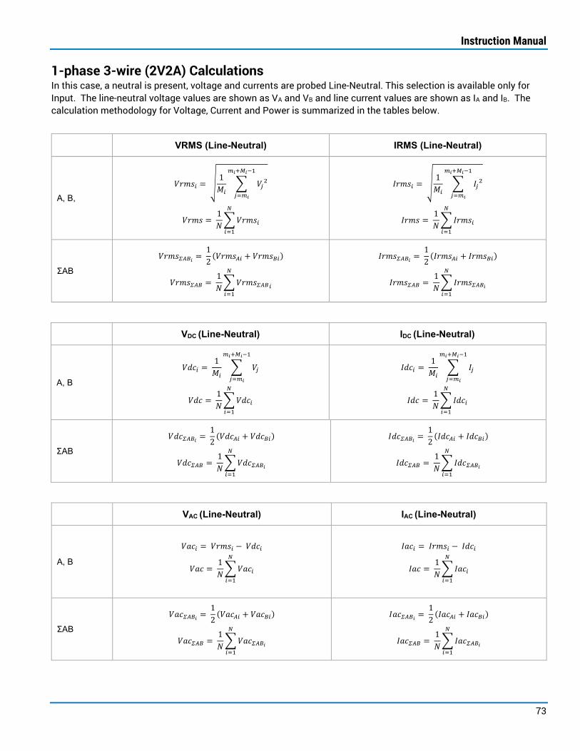
Instruction Manual
73
1-phase 3-wire (2V2A) Calculations In this case, a neutral is present, voltage and currents are probed Line-Neutral. This selection is available only for Input. The line-neutral voltage values are shown as VA and VB and line current values are shown as IA and IB. The calculation methodology for Voltage, Current and Power is summarized in the tables below.
VRMS (Line-Neutral) IRMS (Line-Neutral)
A, B, 𝑉𝑉𝑎𝑎𝑎𝑎𝑉𝑉𝑖𝑖 = �
1𝑀𝑀𝑖𝑖
� 𝑉𝑉𝑗𝑗2𝑚𝑚𝑖𝑖+𝑀𝑀𝑖𝑖−1
𝑗𝑗=𝑚𝑚𝑖𝑖
𝑉𝑉𝑎𝑎𝑎𝑎𝑉𝑉 = 1𝑁𝑁�𝑉𝑉𝑎𝑎𝑎𝑎𝑉𝑉𝑖𝑖
𝑁𝑁
𝑖𝑖=1
𝐼𝐼𝑎𝑎𝑎𝑎𝑉𝑉𝑖𝑖 = �1𝑀𝑀𝑖𝑖
� 𝐼𝐼𝑗𝑗2𝑚𝑚𝑖𝑖+𝑀𝑀𝑖𝑖−1
𝑗𝑗=𝑚𝑚𝑖𝑖
𝐼𝐼𝑎𝑎𝑎𝑎𝑉𝑉 = 1𝑁𝑁�𝐼𝐼𝑎𝑎𝑎𝑎𝑉𝑉𝑖𝑖
𝑁𝑁
𝑖𝑖=1
ΣAB
𝑉𝑉𝑎𝑎𝑎𝑎𝑉𝑉𝛴𝛴𝛴𝛴𝛴𝛴𝑖𝑖 = 12
(𝑉𝑉𝑎𝑎𝑎𝑎𝑉𝑉𝛴𝛴𝑖𝑖 + 𝑉𝑉𝑎𝑎𝑎𝑎𝑉𝑉𝛴𝛴𝑖𝑖)
𝑉𝑉𝑎𝑎𝑎𝑎𝑉𝑉𝛴𝛴𝛴𝛴𝛴𝛴 = 1𝑁𝑁�𝑉𝑉𝑎𝑎𝑎𝑎𝑉𝑉𝛴𝛴𝛴𝛴𝛴𝛴𝑖𝑖
𝑁𝑁
𝑖𝑖=1
𝐼𝐼𝑎𝑎𝑎𝑎𝑉𝑉𝛴𝛴𝛴𝛴𝛴𝛴𝑖𝑖 = 12
(𝐼𝐼𝑎𝑎𝑎𝑎𝑉𝑉𝛴𝛴𝑖𝑖 + 𝐼𝐼𝑎𝑎𝑎𝑎𝑉𝑉𝛴𝛴𝑖𝑖)
𝐼𝐼𝑎𝑎𝑎𝑎𝑉𝑉𝛴𝛴𝛴𝛴𝛴𝛴 = 1𝑁𝑁�𝐼𝐼𝑎𝑎𝑎𝑎𝑉𝑉𝛴𝛴𝛴𝛴𝛴𝛴𝑖𝑖
𝑁𝑁
𝑖𝑖=1
VDC (Line-Neutral) IDC (Line-Neutral)
A, B
𝑉𝑉𝑜𝑜𝐸𝐸𝑖𝑖 = 1𝑀𝑀𝑖𝑖
� 𝑉𝑉𝑗𝑗
𝑚𝑚𝑖𝑖+𝑀𝑀𝑖𝑖−1
𝑗𝑗=𝑚𝑚𝑖𝑖
𝑉𝑉𝑜𝑜𝐸𝐸 = 1𝑁𝑁�𝑉𝑉𝑜𝑜𝐸𝐸𝑖𝑖
𝑁𝑁
𝑖𝑖=1
𝐼𝐼𝑜𝑜𝐸𝐸𝑖𝑖 = 1𝑀𝑀𝑖𝑖
� 𝐼𝐼𝑗𝑗
𝑚𝑚𝑖𝑖+𝑀𝑀𝑖𝑖−1
𝑗𝑗=𝑚𝑚𝑖𝑖
𝐼𝐼𝑜𝑜𝐸𝐸 = 1𝑁𝑁�𝐼𝐼𝑜𝑜𝐸𝐸𝑖𝑖
𝑁𝑁
𝑖𝑖=1
ΣAB
𝑉𝑉𝑜𝑜𝐸𝐸𝛴𝛴𝛴𝛴𝛴𝛴𝑖𝑖 = 12
(𝑉𝑉𝑜𝑜𝐸𝐸𝛴𝛴𝑖𝑖 + 𝑉𝑉𝑜𝑜𝐸𝐸𝛴𝛴𝑖𝑖)
𝑉𝑉𝑜𝑜𝐸𝐸𝛴𝛴𝛴𝛴𝛴𝛴 = 1𝑁𝑁�𝑉𝑉𝑜𝑜𝐸𝐸𝛴𝛴𝛴𝛴𝛴𝛴𝑖𝑖
𝑁𝑁
𝑖𝑖=1
𝐼𝐼𝑜𝑜𝐸𝐸𝛴𝛴𝛴𝛴𝛴𝛴𝑖𝑖 = 12
(𝐼𝐼𝑜𝑜𝐸𝐸𝛴𝛴𝑖𝑖 + 𝐼𝐼𝑜𝑜𝐸𝐸𝛴𝛴𝑖𝑖)
𝐼𝐼𝑜𝑜𝐸𝐸𝛴𝛴𝛴𝛴𝛴𝛴 = 1𝑁𝑁�𝐼𝐼𝑜𝑜𝐸𝐸𝛴𝛴𝛴𝛴𝛴𝛴𝑖𝑖
𝑁𝑁
𝑖𝑖=1
VAC (Line-Neutral) IAC (Line-Neutral)
A, B
𝑉𝑉𝐸𝐸𝐸𝐸𝑖𝑖 = 𝑉𝑉𝑎𝑎𝑎𝑎𝑉𝑉𝑖𝑖 − 𝑉𝑉𝑜𝑜𝐸𝐸𝑖𝑖
𝑉𝑉𝐸𝐸𝐸𝐸 = 1𝑁𝑁�𝑉𝑉𝐸𝐸𝐸𝐸𝑖𝑖
𝑁𝑁
𝑖𝑖=1
𝐼𝐼𝐸𝐸𝐸𝐸𝑖𝑖 = 𝐼𝐼𝑎𝑎𝑎𝑎𝑉𝑉𝑖𝑖 − 𝐼𝐼𝑜𝑜𝐸𝐸𝑖𝑖
𝐼𝐼𝐸𝐸𝐸𝐸 = 1𝑁𝑁�𝐼𝐼𝐸𝐸𝐸𝐸𝑖𝑖
𝑁𝑁
𝑖𝑖=1
ΣAB
𝑉𝑉𝐸𝐸𝐸𝐸𝛴𝛴𝛴𝛴𝛴𝛴𝑖𝑖 = 12
(𝑉𝑉𝐸𝐸𝐸𝐸𝛴𝛴𝑖𝑖 + 𝑉𝑉𝐸𝐸𝐸𝐸𝛴𝛴𝑖𝑖)
𝑉𝑉𝐸𝐸𝐸𝐸𝛴𝛴𝛴𝛴𝛴𝛴 = 1𝑁𝑁�𝑉𝑉𝐸𝐸𝐸𝐸𝛴𝛴𝛴𝛴𝛴𝛴𝑖𝑖
𝑁𝑁
𝑖𝑖=1
𝐼𝐼𝐸𝐸𝐸𝐸𝛴𝛴𝛴𝛴𝛴𝛴𝑖𝑖 = 12
(𝐼𝐼𝐸𝐸𝐸𝐸𝛴𝛴𝑖𝑖 + 𝐼𝐼𝐸𝐸𝐸𝐸𝛴𝛴𝑖𝑖)
𝐼𝐼𝐸𝐸𝐸𝐸𝛴𝛴𝛴𝛴𝛴𝛴 = 1𝑁𝑁�𝐼𝐼𝐸𝐸𝐸𝐸𝛴𝛴𝛴𝛴𝛴𝛴𝑖𝑖
𝑁𝑁
𝑖𝑖=1

3-phase Power Analysis Software
74
VPK+, VPK-, VPK-PK (Line-Neutral) IPK+, IPK-, IPK-PK (Line-Neutral)
A, B
𝑉𝑉𝑐𝑐𝑉𝑉⁺𝑖𝑖 = max𝑗𝑗=𝑚𝑚𝑖𝑖 𝑡𝑡𝑡𝑡 𝑚𝑚𝑖𝑖+𝑀𝑀𝑖𝑖−1
𝑉𝑉𝑗𝑗
𝑉𝑉𝑐𝑐𝑉𝑉⁻𝑖𝑖 = min𝑗𝑗=𝑚𝑚𝑖𝑖 𝑡𝑡𝑡𝑡 𝑚𝑚𝑖𝑖+𝑀𝑀𝑖𝑖−1
𝑉𝑉𝑗𝑗
𝑉𝑉𝑐𝑐𝑉𝑉⎼𝑐𝑐𝑉𝑉𝑖𝑖 = 𝑉𝑉𝑐𝑐𝑉𝑉⁺𝑖𝑖 − 𝑉𝑉𝑐𝑐𝑉𝑉⁻𝑖𝑖 𝑉𝑉𝑐𝑐𝑉𝑉+ = max
𝑖𝑖=1 𝑡𝑡𝑡𝑡 𝑁𝑁 𝑉𝑉𝑐𝑐𝑉𝑉⁺𝑖𝑖
𝑉𝑉𝑐𝑐𝑉𝑉⁻ = min𝑖𝑖=1 𝑡𝑡𝑡𝑡 𝑁𝑁
𝑉𝑉𝑐𝑐𝑉𝑉⁻𝑖𝑖
𝑉𝑉𝑐𝑐𝑉𝑉⎼𝑐𝑐𝑉𝑉 = max𝑖𝑖=1 𝑡𝑡𝑡𝑡 𝑁𝑁
𝑉𝑉𝑐𝑐𝑉𝑉⎼𝑐𝑐𝑉𝑉𝑖𝑖
𝐼𝐼𝑐𝑐𝑉𝑉⁺𝑖𝑖 = max𝑗𝑗=𝑚𝑚𝑖𝑖 𝑡𝑡𝑡𝑡 𝑚𝑚𝑖𝑖+𝑀𝑀𝑖𝑖−1
𝐼𝐼𝑗𝑗
𝐼𝐼𝑐𝑐𝑉𝑉⁻𝑖𝑖 = min𝑗𝑗=𝑚𝑚𝑖𝑖 𝑡𝑡𝑡𝑡 𝑚𝑚𝑖𝑖+𝑀𝑀𝑖𝑖−1
𝐼𝐼𝑗𝑗
𝐼𝐼𝑐𝑐𝑉𝑉⎼𝑐𝑐𝑉𝑉𝑖𝑖 = 𝐼𝐼𝑐𝑐𝑉𝑉⁺𝑖𝑖 − 𝐼𝐼𝑐𝑐𝑉𝑉⁻𝑖𝑖 𝐼𝐼𝑐𝑐𝑉𝑉+ = max
𝑖𝑖=1 𝑡𝑡𝑡𝑡 𝑁𝑁 𝐼𝐼𝑐𝑐𝑉𝑉⁺𝑖𝑖
𝐼𝐼𝑐𝑐𝑉𝑉⁻ = min𝑖𝑖=1 𝑡𝑡𝑡𝑡 𝑁𝑁
𝐼𝐼𝑐𝑐𝑉𝑉⁻𝑖𝑖
𝐼𝐼𝑐𝑐𝑉𝑉⎼𝑐𝑐𝑉𝑉 = max𝑖𝑖=1 𝑡𝑡𝑡𝑡 𝑁𝑁
𝐼𝐼𝑐𝑐𝑉𝑉⎼𝑐𝑐𝑉𝑉𝑖𝑖
ΣAB
𝑉𝑉𝑐𝑐𝑉𝑉+𝛴𝛴𝛴𝛴𝛴𝛴𝑖𝑖 = max�𝑉𝑉𝑐𝑐𝑉𝑉+𝛴𝛴𝑖𝑖 ,𝑉𝑉𝑐𝑐𝑉𝑉+𝛴𝛴𝑖𝑖�
𝑉𝑉𝑐𝑐𝑉𝑉⁻𝛴𝛴𝛴𝛴𝛴𝛴𝑖𝑖 = min�𝑉𝑉𝑐𝑐𝑉𝑉⁻𝛴𝛴𝑖𝑖 ,𝑉𝑉𝑐𝑐𝑉𝑉⁻𝛴𝛴𝑖𝑖�
𝑉𝑉𝑐𝑐𝑉𝑉⎼𝑐𝑐𝑉𝑉𝛴𝛴𝛴𝛴𝛴𝛴𝑖𝑖 = max(𝑉𝑉𝑐𝑐𝑉𝑉⎼𝑐𝑐𝑉𝑉𝛴𝛴𝑖𝑖 ,𝑉𝑉𝑐𝑐𝑉𝑉⎼𝑐𝑐𝑉𝑉𝛴𝛴𝑖𝑖) 𝑉𝑉𝑐𝑐𝑉𝑉+𝛴𝛴𝛴𝛴𝛴𝛴 = max
𝑖𝑖=1 𝑡𝑡𝑡𝑡 𝑁𝑁 𝑉𝑉𝑐𝑐𝑉𝑉+𝛴𝛴𝛴𝛴𝛴𝛴𝑖𝑖
𝑉𝑉𝑐𝑐𝑉𝑉⁻𝛴𝛴𝛴𝛴𝛴𝛴 = max𝑖𝑖=1 𝑡𝑡𝑡𝑡 𝑁𝑁
𝑉𝑉𝑐𝑐𝑉𝑉⁻𝛴𝛴𝛴𝛴𝛴𝛴𝑖𝑖
𝑉𝑉𝑐𝑐𝑉𝑉⎼𝑐𝑐𝑉𝑉𝛴𝛴𝛴𝛴𝛴𝛴 = max𝑖𝑖=1 𝑡𝑡𝑡𝑡 𝑁𝑁
𝑉𝑉𝑐𝑐𝑉𝑉⎼𝑐𝑐𝑉𝑉𝛴𝛴𝛴𝛴𝛴𝛴𝑖𝑖
𝐼𝐼𝑐𝑐𝑉𝑉+𝛴𝛴𝛴𝛴𝛴𝛴𝑖𝑖 = max�𝐼𝐼𝑐𝑐𝑉𝑉+𝛴𝛴𝑖𝑖 , 𝐼𝐼𝑐𝑐𝑉𝑉+𝛴𝛴𝑖𝑖�
𝐼𝐼𝑐𝑐𝑉𝑉⁻𝛴𝛴𝛴𝛴𝛴𝛴𝑖𝑖 = min�𝐼𝐼𝑐𝑐𝑉𝑉⁻𝛴𝛴𝑖𝑖 , 𝐼𝐼𝑐𝑐𝑉𝑉⁻𝛴𝛴𝑖𝑖�
𝐼𝐼𝑐𝑐𝑉𝑉⎼𝑐𝑐𝑉𝑉𝛴𝛴𝛴𝛴𝛴𝛴𝑖𝑖 = max(𝐼𝐼𝑐𝑐𝑉𝑉⎼𝑐𝑐𝑉𝑉𝛴𝛴𝑖𝑖 , 𝐼𝐼𝑐𝑐𝑉𝑉⎼𝑐𝑐𝑉𝑉𝛴𝛴𝑖𝑖) 𝐼𝐼𝑐𝑐𝑉𝑉+𝛴𝛴𝛴𝛴𝛴𝛴 = max
𝑖𝑖=1 𝑡𝑡𝑡𝑡 𝑁𝑁 𝐼𝐼𝑐𝑐𝑉𝑉+𝛴𝛴𝛴𝛴𝛴𝛴𝑖𝑖
𝐼𝐼𝑐𝑐𝑉𝑉⁻𝛴𝛴𝛴𝛴𝛴𝛴 = max𝑖𝑖=1 𝑡𝑡𝑡𝑡 𝑁𝑁
𝐼𝐼𝑐𝑐𝑉𝑉⁻𝛴𝛴𝛴𝛴𝛴𝛴𝑖𝑖
𝐼𝐼𝑐𝑐𝑉𝑉⎼𝑐𝑐𝑉𝑉𝛴𝛴𝛴𝛴𝛴𝛴 = max𝑖𝑖=1 𝑡𝑡𝑡𝑡 𝑁𝑁
𝐼𝐼𝑐𝑐𝑉𝑉⎼𝑐𝑐𝑉𝑉𝛴𝛴𝛴𝛴𝛴𝛴𝑖𝑖
VCF (Line-Neutral) ICF (Line-Neutral)
A, B 𝑉𝑉𝐸𝐸𝑉𝑉𝑖𝑖 =
�max� �𝑉𝑉𝑐𝑐𝑉𝑉+𝑖𝑖�, �𝑉𝑉𝑐𝑐𝑉𝑉−𝑖𝑖 �� �
𝑉𝑉𝐸𝐸𝐸𝐸𝑖𝑖
𝑉𝑉𝐸𝐸𝑉𝑉 = max𝑖𝑖=1 𝑡𝑡𝑡𝑡 𝑁𝑁
𝑉𝑉𝐸𝐸𝑉𝑉𝑖𝑖
𝐼𝐼𝐸𝐸𝑉𝑉𝑖𝑖 =�max� �𝐼𝐼𝑐𝑐𝑉𝑉+𝑖𝑖�, �𝐼𝐼𝑐𝑐𝑉𝑉
−𝑖𝑖 �� �
𝐼𝐼𝐸𝐸𝐸𝐸𝑖𝑖
𝐼𝐼𝐸𝐸𝑉𝑉 = max𝑖𝑖=1 𝑡𝑡𝑡𝑡 𝑁𝑁
𝐼𝐼𝐸𝐸𝑉𝑉𝑖𝑖
ΣAB No calculation is made for this measurement and source No calculation is made for this measurement and source
P S Q
A, B
𝑃𝑃𝑖𝑖 = 1𝑀𝑀𝑖𝑖
� 𝑉𝑉𝑗𝑗 ∗ 𝐼𝐼𝑗𝑗
𝑚𝑚𝑖𝑖+𝑀𝑀𝑖𝑖−1
𝑗𝑗=𝑚𝑚𝑖𝑖
𝑃𝑃 =1𝑁𝑁�𝑃𝑃𝑖𝑖
𝑁𝑁
𝑖𝑖=1
𝑆𝑆𝑖𝑖 = 𝑉𝑉𝑎𝑎𝑎𝑎𝑉𝑉𝑖𝑖 ∗ 𝐼𝐼𝑎𝑎𝑎𝑎𝑉𝑉𝑖𝑖
𝑆𝑆 = 1𝑁𝑁�𝑆𝑆𝑖𝑖
𝑁𝑁
𝑖𝑖=1
𝑄𝑄𝑖𝑖 = �𝑆𝑆𝑖𝑖2 − 𝑃𝑃𝑖𝑖2
sign of Qi is positive if the fundamental voltage vector leads the
fundamental current vector
𝑄𝑄 = 1𝑁𝑁�𝑄𝑄𝑖𝑖
𝑁𝑁
𝑖𝑖=1
ΣAB
𝑃𝑃𝛴𝛴𝛴𝛴𝛴𝛴𝛴𝛴𝑖𝑖 = 𝑃𝑃𝛴𝛴𝑖𝑖 + 𝑃𝑃𝛴𝛴𝑖𝑖
𝑃𝑃𝛴𝛴𝛴𝛴𝛴𝛴𝛴𝛴 = 1𝑁𝑁�𝑃𝑃𝛴𝛴𝛴𝛴𝛴𝛴𝛴𝛴𝑖𝑖
𝑁𝑁
𝑖𝑖=1
𝑆𝑆𝛴𝛴𝛴𝛴𝛴𝛴𝛴𝛴𝑖𝑖 = 𝑆𝑆𝛴𝛴𝑖𝑖 + 𝑆𝑆𝛴𝛴𝑖𝑖
𝑆𝑆𝛴𝛴𝛴𝛴𝛴𝛴𝛴𝛴 = 1𝑁𝑁�𝑆𝑆𝛴𝛴𝛴𝛴𝛴𝛴𝛴𝛴𝑖𝑖
𝑁𝑁
𝑖𝑖=1
𝑄𝑄𝛴𝛴𝛴𝛴𝛴𝛴𝛴𝛴𝑖𝑖 = 𝑄𝑄𝛴𝛴𝑖𝑖 + 𝑄𝑄𝛴𝛴𝑖𝑖
𝑄𝑄𝛴𝛴𝛴𝛴𝛴𝛴𝛴𝛴 = 1𝑁𝑁�𝑄𝑄𝛴𝛴𝛴𝛴𝛴𝛴𝛴𝛴𝑖𝑖
𝑁𝑁
𝑖𝑖=1
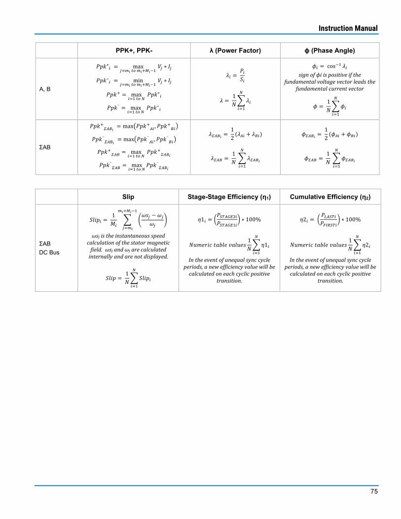
Instruction Manual
75
PPK+, PPK- λ (Power Factor) ϕ (Phase Angle)
A, B
𝑃𝑃𝑐𝑐𝑉𝑉⁺𝑖𝑖 = max𝑗𝑗=𝑚𝑚𝑖𝑖 𝑡𝑡𝑡𝑡 𝑚𝑚𝑖𝑖+𝑀𝑀𝑖𝑖−1
𝑉𝑉𝑗𝑗 ∗ 𝐼𝐼𝑗𝑗
𝑃𝑃𝑐𝑐𝑉𝑉⁻𝑖𝑖 = min𝑗𝑗=𝑚𝑚𝑖𝑖 𝑡𝑡𝑡𝑡 𝑚𝑚𝑖𝑖+𝑀𝑀𝑖𝑖−1
𝑉𝑉𝑗𝑗 ∗ 𝐼𝐼𝑗𝑗
𝑃𝑃𝑐𝑐𝑉𝑉+ = max𝑖𝑖=1 𝑡𝑡𝑡𝑡 𝑁𝑁
𝑃𝑃𝑐𝑐𝑉𝑉⁺𝑖𝑖
𝑃𝑃𝑐𝑐𝑉𝑉⁻ = max𝑖𝑖=1 𝑡𝑡𝑡𝑡 𝑁𝑁
𝑃𝑃𝑐𝑐𝑉𝑉⁻𝑖𝑖
𝜆𝜆𝑖𝑖 = 𝑃𝑃𝑖𝑖𝑆𝑆𝑖𝑖
𝜆𝜆 = 1𝑁𝑁�𝜆𝜆𝑖𝑖
𝑁𝑁
𝑖𝑖=1
𝜙𝜙𝑖𝑖 = cos−1 𝜆𝜆𝑖𝑖 sign of ϕi is positive if the
fundamental voltage vector leads the fundamental current vector
𝜙𝜙 = 1𝑁𝑁�𝜙𝜙𝑖𝑖
𝑁𝑁
𝑖𝑖=1
ΣAB
𝑃𝑃𝑐𝑐𝑉𝑉+𝛴𝛴𝛴𝛴𝛴𝛴𝑖𝑖 = max�𝑃𝑃𝑐𝑐𝑉𝑉+𝛴𝛴𝑖𝑖 ,𝑃𝑃𝑐𝑐𝑉𝑉+𝛴𝛴𝑖𝑖�
𝑃𝑃𝑐𝑐𝑉𝑉⁻𝛴𝛴𝛴𝛴𝛴𝛴𝑖𝑖 = max�𝑃𝑃𝑐𝑐𝑉𝑉⁻𝛴𝛴𝑖𝑖 ,𝑃𝑃𝑐𝑐𝑉𝑉⁻𝛴𝛴𝑖𝑖�
𝑃𝑃𝑐𝑐𝑉𝑉+𝛴𝛴𝛴𝛴𝛴𝛴 = max𝑖𝑖=1 𝑡𝑡𝑡𝑡 𝑁𝑁
𝑃𝑃𝑐𝑐𝑉𝑉+𝛴𝛴𝛴𝛴𝛴𝛴𝑖𝑖
𝑃𝑃𝑐𝑐𝑉𝑉⁻𝛴𝛴𝛴𝛴𝛴𝛴 = max𝑖𝑖=1 𝑡𝑡𝑡𝑡 𝑁𝑁
𝑃𝑃𝑐𝑐𝑉𝑉⁻𝛴𝛴𝛴𝛴𝛴𝛴𝑖𝑖
𝜆𝜆𝛴𝛴𝛴𝛴𝛴𝛴𝑖𝑖 = 12 (𝜆𝜆𝛴𝛴𝑖𝑖 + 𝜆𝜆𝛴𝛴𝑖𝑖)
𝜆𝜆𝛴𝛴𝛴𝛴𝛴𝛴 = 1𝑁𝑁 �𝜆𝜆𝛴𝛴𝛴𝛴𝛴𝛴𝑖𝑖
𝑁𝑁
𝑖𝑖=1
𝜙𝜙𝛴𝛴𝛴𝛴𝛴𝛴𝑖𝑖 = 12 (𝜙𝜙𝛴𝛴𝑖𝑖 + 𝜙𝜙𝛴𝛴𝑖𝑖)
𝜙𝜙𝛴𝛴𝛴𝛴𝛴𝛴 = 1𝑁𝑁 �𝜙𝜙𝛴𝛴𝛴𝛴𝛴𝛴𝑖𝑖
𝑁𝑁
𝑖𝑖=1
Slip Stage-Stage Efficiency (η1) Cumulative Efficiency (η2)
ΣAB DC Bus
𝑆𝑆𝐹𝐹𝑎𝑎𝑐𝑐𝑖𝑖 = 1𝑀𝑀𝑖𝑖
� �𝜔𝜔𝑉𝑉𝑗𝑗 − 𝜔𝜔𝑗𝑗
𝜔𝜔𝑗𝑗�
𝑚𝑚𝑖𝑖+𝑀𝑀𝑖𝑖−1
𝑗𝑗=𝑚𝑚𝑖𝑖
ωsj is the instantaneous speed calculation of the stator magnetic
field. ωsj and ωj are calculated internally and are not displayed.
𝑆𝑆𝐹𝐹𝑎𝑎𝑐𝑐 = 1𝑁𝑁�𝑆𝑆𝐹𝐹𝑎𝑎𝑐𝑐𝑖𝑖
𝑁𝑁
𝑖𝑖=1
𝜂𝜂1𝑖𝑖 = �𝑃𝑃𝛴𝛴𝛴𝛴𝛴𝛴𝑆𝑆𝑆𝑆2𝑖𝑖𝑃𝑃𝛴𝛴𝛴𝛴𝛴𝛴𝑆𝑆𝑆𝑆1𝑖𝑖
� ∗ 100%
𝑁𝑁𝐹𝐹𝑎𝑎𝑜𝑜𝑎𝑎𝑎𝑎𝐸𝐸 𝐹𝐹𝐸𝐸𝑡𝑡𝐹𝐹𝑜𝑜 𝑣𝑣𝐸𝐸𝐹𝐹𝐹𝐹𝑜𝑜𝑉𝑉1𝑁𝑁�𝜂𝜂1𝑖𝑖
𝑁𝑁
𝑖𝑖=1
In the event of unequal sync cycle periods, a new efficiency value will be
calculated on each cyclic positive transition.
𝜂𝜂2𝑖𝑖 = �𝑃𝑃𝐿𝐿𝛴𝛴𝛴𝛴𝛴𝛴𝑖𝑖𝑃𝑃𝐹𝐹𝐹𝐹𝛴𝛴𝛴𝛴𝛴𝛴𝑖𝑖
� ∗ 100%
𝑁𝑁𝐹𝐹𝑎𝑎𝑜𝑜𝑎𝑎𝑎𝑎𝐸𝐸 𝐹𝐹𝐸𝐸𝑡𝑡𝐹𝐹𝑜𝑜 𝑣𝑣𝐸𝐸𝐹𝐹𝐹𝐹𝑜𝑜𝑉𝑉1𝑁𝑁�𝜂𝜂2𝑖𝑖
𝑁𝑁
𝑖𝑖=1
In the event of unequal sync cycle periods, a new efficiency value will be
calculated on each cyclic positive transition.

3-phase Power Analysis Software
76
1-phase 2-wire Wiring Configuration Calculations 1-phase 2-wire (1V1A) Input or DC Bus Calculations 1-phase/Half-Bridge (1V1A) Output Calculations 1-phase/Full-Bridge (1V1A) Output Calculations
In this case, a neutral is present, voltage and currents are probed Line-Neutral. These selections are available in Input, DC Bus, or Output. The line-neutral voltage values are shown as VA and VR and line current values are shown as IA and IR. The calculation methodology for Voltage, Current and Power is summarized in the tables below.
VRMS IRMS
A R DC Bus
𝑉𝑉𝑎𝑎𝑎𝑎𝑉𝑉𝑖𝑖 = �1𝑀𝑀𝑖𝑖
� 𝑉𝑉𝑗𝑗2𝑚𝑚𝑖𝑖+𝑀𝑀𝑖𝑖−1
𝑗𝑗=𝑚𝑚𝑖𝑖
𝑉𝑉𝑎𝑎𝑎𝑎𝑉𝑉 = 1𝑁𝑁�𝑉𝑉𝑎𝑎𝑎𝑎𝑉𝑉𝑖𝑖
𝑁𝑁
𝑖𝑖=1
𝐼𝐼𝑎𝑎𝑎𝑎𝑉𝑉𝑖𝑖 = �1𝑀𝑀𝑖𝑖
� 𝐼𝐼𝑗𝑗2𝑚𝑚𝑖𝑖+𝑀𝑀𝑖𝑖−1
𝑗𝑗=𝑚𝑚𝑖𝑖
𝐼𝐼𝑎𝑎𝑎𝑎𝑉𝑉 = 1𝑁𝑁�𝐼𝐼𝑎𝑎𝑎𝑎𝑉𝑉𝑖𝑖
𝑁𝑁
𝑖𝑖=1
VDC IDC
A R DC Bus
𝑉𝑉𝑜𝑜𝐸𝐸𝑖𝑖 = 1𝑀𝑀𝑖𝑖
� 𝑉𝑉𝑗𝑗
𝑚𝑚𝑖𝑖+𝑀𝑀𝑖𝑖−1
𝑗𝑗=𝑚𝑚𝑖𝑖
𝑉𝑉𝑜𝑜𝐸𝐸 = 1𝑁𝑁�𝑉𝑉𝑜𝑜𝐸𝐸𝑖𝑖
𝑁𝑁
𝑖𝑖=1
𝐼𝐼𝑜𝑜𝐸𝐸𝑖𝑖 = 1𝑀𝑀𝑖𝑖
� 𝐼𝐼𝑗𝑗
𝑚𝑚𝑖𝑖+𝑀𝑀𝑖𝑖−1
𝑗𝑗=𝑚𝑚𝑖𝑖
𝐼𝐼𝑜𝑜𝐸𝐸 = 1𝑁𝑁�𝐼𝐼𝑜𝑜𝐸𝐸𝑖𝑖
𝑁𝑁
𝑖𝑖=1
VAC IAC
A R DC Bus
𝑉𝑉𝐸𝐸𝐸𝐸𝑖𝑖 = 𝑉𝑉𝑎𝑎𝑎𝑎𝑉𝑉𝑖𝑖 − 𝑉𝑉𝑜𝑜𝐸𝐸𝑖𝑖
𝑉𝑉𝐸𝐸𝐸𝐸 = 1𝑁𝑁�𝑉𝑉𝐸𝐸𝐸𝐸𝑖𝑖
𝑁𝑁
𝑖𝑖=1
𝐼𝐼𝐸𝐸𝐸𝐸𝑖𝑖 = 𝐼𝐼𝑎𝑎𝑎𝑎𝑉𝑉𝑖𝑖 − 𝐼𝐼𝑜𝑜𝐸𝐸𝑖𝑖
𝐼𝐼𝐸𝐸𝐸𝐸 = 1𝑁𝑁�𝐼𝐼𝐸𝐸𝐸𝐸𝑖𝑖
𝑁𝑁
𝑖𝑖=1
VPK+, VPK-, VPK-PK IPK+, IPK-, IPK-PK
A R DC Bus
𝑉𝑉𝑐𝑐𝑉𝑉⁺𝑖𝑖 = max𝑗𝑗=𝑚𝑚𝑖𝑖 𝑡𝑡𝑡𝑡 𝑚𝑚𝑖𝑖+𝑀𝑀𝑖𝑖−1
𝑉𝑉𝑗𝑗
𝑉𝑉𝑐𝑐𝑉𝑉⁻𝑖𝑖 = min𝑗𝑗=𝑚𝑚𝑖𝑖 𝑡𝑡𝑡𝑡 𝑚𝑚𝑖𝑖+𝑀𝑀𝑖𝑖−1
𝑉𝑉𝑗𝑗
𝑉𝑉𝑐𝑐𝑉𝑉⎼𝑐𝑐𝑉𝑉𝑖𝑖 = 𝑉𝑉𝑐𝑐𝑉𝑉⁺𝑖𝑖 − 𝑉𝑉𝑐𝑐𝑉𝑉⁻𝑖𝑖
𝑉𝑉𝑐𝑐𝑉𝑉+ = max𝑖𝑖=1 𝑡𝑡𝑡𝑡 𝑁𝑁
𝑉𝑉𝑐𝑐𝑉𝑉⁺𝑖𝑖
𝑉𝑉𝑐𝑐𝑉𝑉⁻ = min𝑖𝑖=1 𝑡𝑡𝑡𝑡 𝑁𝑁
𝑉𝑉𝑐𝑐𝑉𝑉⁻𝑖𝑖
𝑉𝑉𝑐𝑐𝑉𝑉⎼𝑐𝑐𝑉𝑉 = max𝑖𝑖=1 𝑡𝑡𝑡𝑡 𝑁𝑁
𝑉𝑉𝑐𝑐𝑉𝑉⎼𝑐𝑐𝑉𝑉𝑖𝑖
𝐼𝐼𝑐𝑐𝑉𝑉⁺𝑖𝑖 = max𝑗𝑗=𝑚𝑚𝑖𝑖 𝑡𝑡𝑡𝑡 𝑚𝑚𝑖𝑖+𝑀𝑀𝑖𝑖−1
𝐼𝐼𝑗𝑗
𝐼𝐼𝑐𝑐𝑉𝑉⁻𝑖𝑖 = min𝑗𝑗=𝑚𝑚𝑖𝑖 𝑡𝑡𝑡𝑡 𝑚𝑚𝑖𝑖+𝑀𝑀𝑖𝑖−1
𝐼𝐼𝑗𝑗
𝐼𝐼𝑐𝑐𝑉𝑉⎼𝑐𝑐𝑉𝑉𝑖𝑖 = 𝐼𝐼𝑐𝑐𝑉𝑉⁺𝑖𝑖 − 𝐼𝐼𝑐𝑐𝑉𝑉⁻𝑖𝑖
𝐼𝐼𝑐𝑐𝑉𝑉+ = max𝑖𝑖=1 𝑡𝑡𝑡𝑡 𝑁𝑁
𝐼𝐼𝑐𝑐𝑉𝑉⁺𝑖𝑖
𝐼𝐼𝑐𝑐𝑉𝑉⁻ = min𝑖𝑖=1 𝑡𝑡𝑡𝑡 𝑁𝑁
𝐼𝐼𝑐𝑐𝑉𝑉⁻𝑖𝑖
𝐼𝐼𝑐𝑐𝑉𝑉⎼𝑐𝑐𝑉𝑉 = max𝑖𝑖=1 𝑡𝑡𝑡𝑡 𝑁𝑁
𝐼𝐼𝑐𝑐𝑉𝑉⎼𝑐𝑐𝑉𝑉𝑖𝑖

Instruction Manual
77
VCF ICF
A R DC Bus
𝑉𝑉𝐸𝐸𝑉𝑉𝑖𝑖 =�max� �𝑉𝑉𝑐𝑐𝑉𝑉+𝑖𝑖�, �𝑉𝑉𝑐𝑐𝑉𝑉
−𝑖𝑖 �� �
𝑉𝑉𝐸𝐸𝐸𝐸𝑖𝑖
𝑉𝑉𝐸𝐸𝑉𝑉 = max𝑖𝑖=1 𝑡𝑡𝑡𝑡 𝑁𝑁
𝑉𝑉𝐸𝐸𝑉𝑉𝑖𝑖
𝐼𝐼𝐸𝐸𝑉𝑉𝑖𝑖 =�max� �𝐼𝐼𝑐𝑐𝑉𝑉+𝑖𝑖�, �𝐼𝐼𝑐𝑐𝑉𝑉
−𝑖𝑖 �� �
𝐼𝐼𝐸𝐸𝐸𝐸𝑖𝑖
𝐼𝐼𝐸𝐸𝑉𝑉 = max𝑖𝑖=1 𝑡𝑡𝑡𝑡 𝑁𝑁
𝐼𝐼𝐸𝐸𝑉𝑉𝑖𝑖
P S Q
A R DC Bus
𝑃𝑃𝑖𝑖 = 1𝑀𝑀𝑖𝑖
� 𝑉𝑉𝑗𝑗 ∗ 𝐼𝐼𝑗𝑗
𝑚𝑚𝑖𝑖+𝑀𝑀𝑖𝑖−1
𝑗𝑗=𝑚𝑚𝑖𝑖
𝑃𝑃 =1𝑁𝑁�𝑃𝑃𝑖𝑖
𝑁𝑁
𝑖𝑖=1
𝑆𝑆𝑖𝑖 = 𝑉𝑉𝑎𝑎𝑎𝑎𝑉𝑉𝑖𝑖 ∗ 𝐼𝐼𝑎𝑎𝑎𝑎𝑉𝑉𝑖𝑖
𝑆𝑆 = 1𝑁𝑁�𝑆𝑆𝑖𝑖
𝑁𝑁
𝑖𝑖=1
𝑎𝑎𝐸𝐸𝑚𝑚𝑎𝑎𝑎𝑎𝐹𝐹𝐹𝐹𝑜𝑜𝑜𝑜 𝑄𝑄𝑖𝑖 = �𝑆𝑆𝑖𝑖2 − 𝑃𝑃𝑖𝑖2
sign of Qi is positive if the fundamental voltage vector leads the
fundamental current vector
𝑄𝑄 = 1𝑁𝑁�𝑄𝑄𝑖𝑖
𝑁𝑁
𝑖𝑖=1
PPK+, PPK- λ (Power Factor) ϕ (Phase Angle)
A R DC Bus
𝑃𝑃𝑐𝑐𝑉𝑉⁺𝑖𝑖 = max𝑗𝑗=𝑚𝑚𝑖𝑖 𝑡𝑡𝑡𝑡 𝑚𝑚𝑖𝑖+𝑀𝑀𝑖𝑖−1
𝑉𝑉𝑗𝑗 ∗ 𝐼𝐼𝑗𝑗
𝑃𝑃𝑐𝑐𝑉𝑉⁻𝑖𝑖 = min𝑗𝑗=𝑚𝑚𝑖𝑖 𝑡𝑡𝑡𝑡 𝑚𝑚𝑖𝑖+𝑀𝑀𝑖𝑖−1
𝑉𝑉𝑗𝑗 ∗ 𝐼𝐼𝑗𝑗
𝑃𝑃𝑐𝑐𝑉𝑉+ = max𝑖𝑖=1 𝑡𝑡𝑡𝑡 𝑁𝑁
𝑃𝑃𝑐𝑐𝑉𝑉⁺𝑖𝑖
𝑃𝑃𝑐𝑐𝑉𝑉⁻ = min𝑖𝑖=1 𝑡𝑡𝑡𝑡 𝑁𝑁
𝑃𝑃𝑐𝑐𝑉𝑉⁻𝑖𝑖
𝜆𝜆𝑖𝑖 = 𝑃𝑃𝑖𝑖𝑆𝑆𝑖𝑖
𝜆𝜆 = 1𝑁𝑁�𝜆𝜆𝑖𝑖
𝑁𝑁
𝑖𝑖=1
𝑎𝑎𝐸𝐸𝑚𝑚𝑎𝑎𝑎𝑎𝐹𝐹𝐹𝐹𝑜𝑜𝑜𝑜 𝜙𝜙𝑖𝑖 = cos−1 𝜆𝜆𝑖𝑖 sign of ϕi is positive if the
fundamental voltage vector leads the fundamental current vector
𝜙𝜙 = 1𝑁𝑁�𝜙𝜙𝑖𝑖
𝑁𝑁
𝑖𝑖=1
Slip Stage-Stage Efficiency (η1) Cumulative Efficiency (η2)
A R DC Bus
𝑆𝑆𝐹𝐹𝑎𝑎𝑐𝑐𝑖𝑖 = 1𝑀𝑀𝑖𝑖
� �𝜔𝜔𝑉𝑉𝑗𝑗 − 𝜔𝜔𝑗𝑗
𝜔𝜔𝑗𝑗�
𝑚𝑚𝑖𝑖+𝑀𝑀𝑖𝑖−1
𝑗𝑗=𝑚𝑚𝑖𝑖
ωsj is the instantaneous speed calculation of the stator magnetic
field. ωsj and ωj are calculated internally and are not displayed.
𝑆𝑆𝐹𝐹𝑎𝑎𝑐𝑐 = 1𝑁𝑁�𝑆𝑆𝐹𝐹𝑎𝑎𝑐𝑐𝑖𝑖
𝑁𝑁
𝑖𝑖=1
𝜂𝜂1𝑖𝑖 = �𝑃𝑃𝛴𝛴𝛴𝛴𝛴𝛴𝑆𝑆𝑆𝑆2𝑖𝑖𝑃𝑃𝛴𝛴𝛴𝛴𝛴𝛴𝑆𝑆𝑆𝑆1𝑖𝑖
� ∗ 100%
𝑁𝑁𝐹𝐹𝑎𝑎𝑜𝑜𝑎𝑎𝑎𝑎𝐸𝐸 𝐹𝐹𝐸𝐸𝑡𝑡𝐹𝐹𝑜𝑜 𝑣𝑣𝐸𝐸𝐹𝐹𝐹𝐹𝑜𝑜𝑉𝑉1𝑁𝑁�𝜂𝜂1𝑖𝑖
𝑁𝑁
𝑖𝑖=1
In the event of unequal sync cycle periods, a new efficiency value will be
calculated on each cyclic positive transition.
𝜂𝜂2𝑖𝑖 = �𝑃𝑃𝐿𝐿𝛴𝛴𝛴𝛴𝛴𝛴𝑖𝑖𝑃𝑃𝐹𝐹𝐹𝐹𝛴𝛴𝛴𝛴𝛴𝛴𝑖𝑖
� ∗ 100%
𝑁𝑁𝐹𝐹𝑎𝑎𝑜𝑜𝑎𝑎𝑎𝑎𝐸𝐸 𝐹𝐹𝐸𝐸𝑡𝑡𝐹𝐹𝑜𝑜 𝑣𝑣𝐸𝐸𝐹𝐹𝐹𝐹𝑜𝑜𝑉𝑉1𝑁𝑁�𝜂𝜂2𝑖𝑖
𝑁𝑁
𝑖𝑖=1
In the event of unequal sync cycle periods, a new efficiency value will be
calculated on each cyclic positive transition.
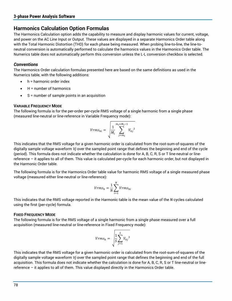
3-phase Power Analysis Software
78
Harmonics Calculation Option Formulas The Harmonics Calculation option adds the capability to measure and display harmonic values for current, voltage, and power on the AC Line Input or Output. These values are displayed in a separate Harmonics Order table along with the Total Harmonic Distortion (THD) for each phase being measured. When probing line-to-line, the line-to-neutral conversion is automatically performed to calculate the harmonics values in the Harmonics Order table. The Numerics table does not automatically perform this conversion unless the L-L conversion checkbox is selected.
Conventions The Harmonics Order calculation formulas presented here are based on the same definitions as used in the Numerics table, with the following additions:
• h = harmonic order index
• H = number of harmonics
• S = number of sample points in an acquisition
VARIABLE FREQUENCY MODE The following formula is for the per-order per-cycle RMS voltage of a single harmonic from a single phase (measured line-neutral or line-reference in Variable Frequency mode):
𝑉𝑉𝑎𝑎𝑎𝑎𝑉𝑉ℎ𝑖𝑖 = �1𝑀𝑀𝑖𝑖
� 𝑉𝑉ℎ𝑗𝑗2𝑚𝑚𝑖𝑖+𝑀𝑀𝑖𝑖−1
𝑗𝑗=𝑚𝑚𝑖𝑖
This indicates that the RMS voltage for a given harmonic order is calculated from the root-sum-of-squares of the digitally sample voltage waveform Vj over the sampled point range that defines the beginning and end of the cycle (period). This formula does not indicate whether the calculation is done for A, B, C, R, S or T line-neutral or line-reference – it applies to all of them. This value is calculated per-cycle for each harmonic order, but not displayed in the Harmonic Order table.
The following formula is for the Harmonics Order table value for harmonic RMS voltage of a single measured phase voltage (measured either line-neutral or line-reference):
𝑉𝑉𝑎𝑎𝑎𝑎𝑉𝑉ℎ =1𝑁𝑁�𝑉𝑉𝑎𝑎𝑎𝑎𝑉𝑉ℎ𝑖𝑖
𝑁𝑁
𝑖𝑖=1
This indicates that the RMS voltage reported in the Harmonic table is the mean value of the N cycles calculated using the first (per-cycle) formula.
FIXED FREQUENCY MODE The following formula is for the RMS voltage of a single harmonic from a single phase measured over a full acquisition (measured line-neutral or line-reference in Fixed Frequency mode):
𝑉𝑉𝑎𝑎𝑎𝑎𝑉𝑉ℎ = �1𝑆𝑆�𝑉𝑉ℎ𝑗𝑗2𝛴𝛴
𝑗𝑗=1
This indicates that the RMS voltage for a given harmonic order is calculated from the root-sum-of-squares of the digitally sample voltage waveform Vj over the sampled point range that defines the beginning and end of the full acquisition. This formula does not indicate whether the calculation is done for A, B, C, R, S or T line-neutral or line-reference – it applies to all of them. This value displayed directly in the Harmonics Order table.
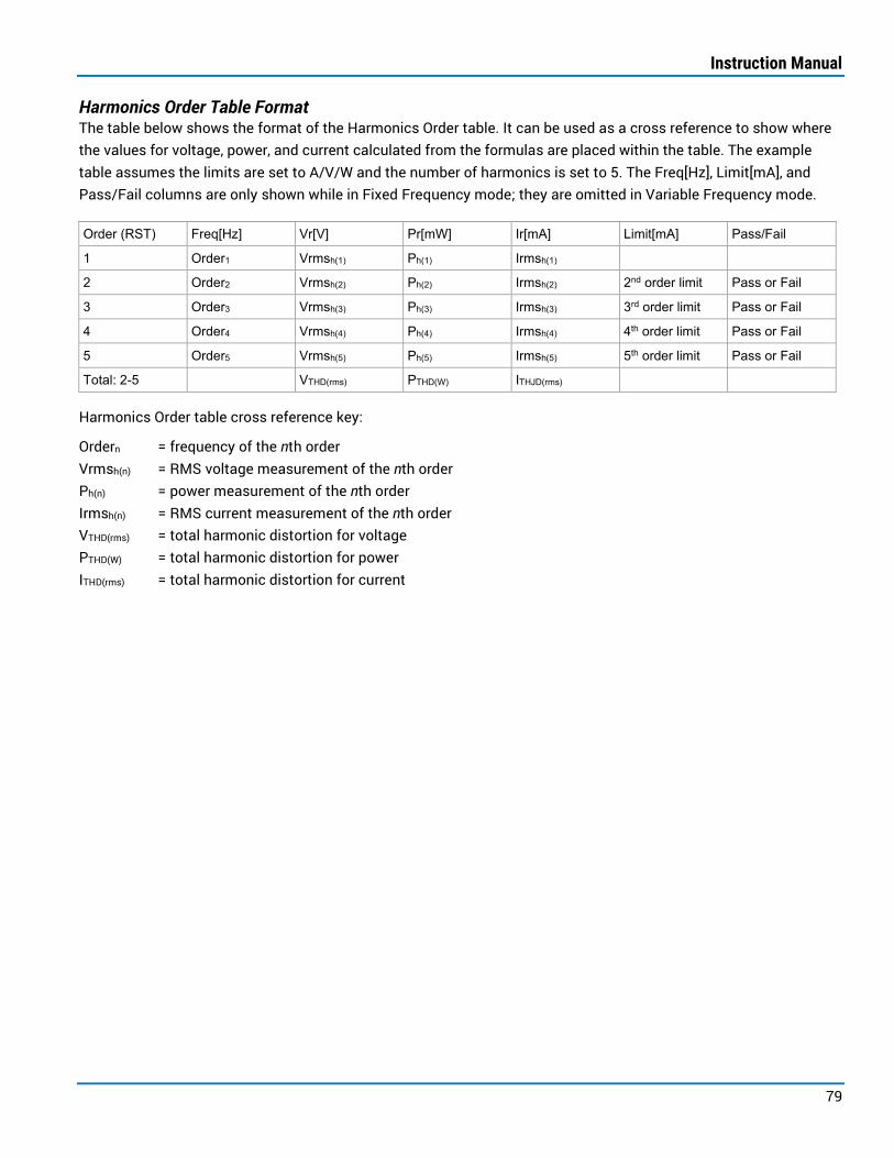
Instruction Manual
79
Harmonics Order Table Format The table below shows the format of the Harmonics Order table. It can be used as a cross reference to show where the values for voltage, power, and current calculated from the formulas are placed within the table. The example table assumes the limits are set to A/V/W and the number of harmonics is set to 5. The Freq[Hz], Limit[mA], and Pass/Fail columns are only shown while in Fixed Frequency mode; they are omitted in Variable Frequency mode.
Order (RST) Freq[Hz] Vr[V] Pr[mW] Ir[mA] Limit[mA] Pass/Fail
1 Order1 Vrmsh(1) Ph(1) Irmsh(1)
2 Order2 Vrmsh(2) Ph(2) Irmsh(2) 2nd order limit Pass or Fail
3 Order3 Vrmsh(3) Ph(3) Irmsh(3) 3rd order limit Pass or Fail
4 Order4 Vrmsh(4) Ph(4) Irmsh(4) 4th order limit Pass or Fail
5 Order5 Vrmsh(5) Ph(5) Irmsh(5) 5th order limit Pass or Fail
Total: 2-5 VTHD(rms) PTHD(W) ITHJD(rms)
Harmonics Order table cross reference key:
Ordern = frequency of the nth order Vrmsh(n) = RMS voltage measurement of the nth order
Ph(n) = power measurement of the nth order Irmsh(n) = RMS current measurement of the nth order VTHD(rms) = total harmonic distortion for voltage PTHD(W) = total harmonic distortion for power ITHD(rms) = total harmonic distortion for current

3-phase Power Analysis Software
80
Harmonics Order Table Calculations The following tables describe the calculations for the Harmonics Order table. These calculations apply to all available wiring diagrams. In cases where the wiring diagram is a Line-Line configuration, the Line-Line to Line-Neutral conversion is automatically applied for these Harmonic Order table calculations.
VARYING FREQUENCY MODE CALCULATIONS
VTHD(Vrms) VTHD(dBµV) VTHD(%)
A, B, C R, S, T 𝑉𝑉𝑎𝑎𝑎𝑎𝑉𝑉ℎ𝑖𝑖 = �
1𝑀𝑀𝑖𝑖
� 𝑉𝑉ℎ𝑗𝑗2𝑚𝑚𝑖𝑖+𝑀𝑀𝑖𝑖−1
𝑗𝑗=𝑚𝑚𝑖𝑖
𝑉𝑉𝑎𝑎𝑎𝑎𝑉𝑉ℎ𝑖𝑖 𝑎𝑎𝑉𝑉 𝐸𝐸𝐸𝐸𝐹𝐹𝐸𝐸𝐹𝐹𝐹𝐹𝐸𝐸𝐹𝐹𝑜𝑜𝑜𝑜 𝑎𝑎𝑎𝑎𝐹𝐹𝑜𝑜𝑎𝑎𝑎𝑎𝐸𝐸𝐹𝐹𝐹𝐹𝑖𝑖 𝐸𝐸𝑎𝑎𝑜𝑜 𝑎𝑎𝑉𝑉 𝑎𝑎𝑎𝑎𝐹𝐹 𝑜𝑜𝑎𝑎𝑉𝑉𝑐𝑐𝐹𝐹𝐸𝐸𝑖𝑖𝑜𝑜𝑜𝑜
𝑉𝑉𝑎𝑎𝑎𝑎𝑉𝑉ℎ =1𝑁𝑁�𝑉𝑉𝑎𝑎𝑎𝑎𝑉𝑉ℎ𝑖𝑖
𝑁𝑁
𝑖𝑖=1
𝑉𝑉𝛴𝛴𝑇𝑇𝑇𝑇(𝑉𝑉𝑉𝑉𝑚𝑚𝑉𝑉) = ��𝑉𝑉𝑎𝑎𝑎𝑎𝑉𝑉ℎ2𝑇𝑇
ℎ=2
See calculation for Vrmsh, first column
𝑉𝑉𝑑𝑑𝛴𝛴𝑑𝑑𝑉𝑉ℎ = 20 ∗ 𝐹𝐹𝑎𝑎𝑚𝑚 (𝑉𝑉𝑎𝑎𝑎𝑎𝑉𝑉ℎ ∗ 106)
𝑉𝑉𝛴𝛴𝑇𝑇𝑇𝑇(𝑑𝑑𝛴𝛴𝑑𝑑𝑉𝑉) = ��𝑉𝑉𝑑𝑑𝛴𝛴𝑑𝑑𝑉𝑉ℎ2
𝑇𝑇
ℎ=2
See calculation for Vrmsh, first column
𝑉𝑉%ℎ =𝑉𝑉𝑎𝑎𝑎𝑎𝑉𝑉ℎ𝑉𝑉𝑎𝑎𝑎𝑎𝑉𝑉ℎ(1)
∗ 100
𝑉𝑉𝛴𝛴𝑇𝑇𝑇𝑇(%) = ��𝑉𝑉%2ℎ
𝑇𝑇
ℎ=2
ITHD(A) ITHD(dBµA) ITHD(%) A, B, C R, S, T 𝐼𝐼𝑎𝑎𝑎𝑎𝑉𝑉ℎ𝑖𝑖 = �
1𝑀𝑀𝑖𝑖
� 𝐼𝐼ℎ𝑗𝑗2𝑚𝑚𝑖𝑖+𝑀𝑀𝑖𝑖−1
𝑗𝑗=𝑚𝑚𝑖𝑖
𝐼𝐼𝑎𝑎𝑎𝑎𝑉𝑉ℎ𝑖𝑖 𝑎𝑎𝑉𝑉 𝐸𝐸𝐸𝐸𝐹𝐹𝐸𝐸𝐹𝐹𝐹𝐹𝐸𝐸𝐹𝐹𝑜𝑜𝑜𝑜 𝑎𝑎𝑎𝑎𝐹𝐹𝑜𝑜𝑎𝑎𝑎𝑎𝐸𝐸𝐹𝐹𝐹𝐹𝑖𝑖 𝐸𝐸𝑎𝑎𝑜𝑜 𝑎𝑎𝑉𝑉 𝑎𝑎𝑎𝑎𝐹𝐹 𝑜𝑜𝑎𝑎𝑉𝑉𝑐𝑐𝐹𝐹𝐸𝐸𝑖𝑖𝑜𝑜𝑜𝑜
𝐼𝐼𝑎𝑎𝑎𝑎𝑉𝑉ℎ =1𝑁𝑁�𝐼𝐼𝑎𝑎𝑎𝑎𝑉𝑉ℎ𝑖𝑖
𝑁𝑁
𝑖𝑖=1
𝐼𝐼𝛴𝛴𝑇𝑇𝑇𝑇(𝑉𝑉𝑚𝑚𝑉𝑉) = ��𝐼𝐼𝑎𝑎𝑎𝑎𝑉𝑉ℎ2𝑇𝑇
ℎ=2
See calculation for Irmsh, first column
𝐼𝐼𝑑𝑑𝛴𝛴µ𝛴𝛴ℎ = 20 ∗ 𝐹𝐹𝑎𝑎𝑚𝑚 (𝐼𝐼𝑎𝑎𝑎𝑎𝑉𝑉ℎ ∗ 106)
𝐼𝐼𝛴𝛴𝑇𝑇𝑇𝑇(𝑑𝑑𝛴𝛴µ𝛴𝛴) = ��𝐼𝐼𝑑𝑑𝛴𝛴µ𝛴𝛴ℎ2
𝑇𝑇
ℎ=2
See calculation for Irmsh, first column
𝐼𝐼% =𝐼𝐼𝑎𝑎𝑎𝑎𝑉𝑉ℎ𝐼𝐼𝑎𝑎𝑎𝑎𝑉𝑉ℎ(1)
∗ 100
𝐼𝐼𝛴𝛴𝑇𝑇𝑇𝑇(%) = ��𝐼𝐼%2 ℎ
𝑇𝑇
ℎ=2
PTHD(W) PTHD(dBµW) PTHD(%) A, B, C R, S, T 𝑃𝑃ℎ𝑖𝑖 =
1𝑀𝑀𝑖𝑖
� 𝑉𝑉ℎ𝑗𝑗 ∗ 𝐼𝐼ℎ𝑗𝑗
𝑚𝑚𝑖𝑖+𝑀𝑀𝑖𝑖−1
𝑗𝑗=𝑚𝑚𝑖𝑖
𝑃𝑃ℎ𝑖𝑖 𝑎𝑎𝑉𝑉 𝐸𝐸𝐸𝐸𝐹𝐹𝐸𝐸𝐹𝐹𝐹𝐹𝐸𝐸𝐹𝐹𝑜𝑜𝑜𝑜 𝑎𝑎𝑎𝑎𝐹𝐹𝑜𝑜𝑎𝑎𝑎𝑎𝐸𝐸𝐹𝐹𝐹𝐹𝑖𝑖 𝐸𝐸𝑎𝑎𝑜𝑜 𝑎𝑎𝑉𝑉 𝑎𝑎𝑎𝑎𝐹𝐹 𝑜𝑜𝑎𝑎𝑉𝑉𝑐𝑐𝐹𝐹𝐸𝐸𝑖𝑖𝑜𝑜𝑜𝑜
𝑃𝑃ℎ =1𝑁𝑁�𝑃𝑃ℎ𝑖𝑖
𝑁𝑁
𝑖𝑖=1
𝑃𝑃𝛴𝛴𝑇𝑇𝑇𝑇(𝑊𝑊) = �𝑃𝑃ℎ
𝑇𝑇
ℎ=2
See calculation for Ph, first column
𝑃𝑃𝑑𝑑𝛴𝛴ℎ = 20 ∗ 𝐹𝐹𝑎𝑎𝑚𝑚 (𝑃𝑃ℎ ∗ 106)
𝑃𝑃𝛴𝛴𝑇𝑇𝑇𝑇(𝑑𝑑𝛴𝛴µ𝑊𝑊) = �𝑃𝑃𝑑𝑑𝛴𝛴µ𝑊𝑊ℎ
𝑇𝑇
ℎ=2
See calculation for Ph, first column
𝑃𝑃% =𝑃𝑃ℎ𝑃𝑃ℎ(1)
∗ 100
𝑃𝑃𝛴𝛴𝑇𝑇𝑇𝑇(%) = �𝑃𝑃%ℎ
𝑇𝑇
ℎ=2
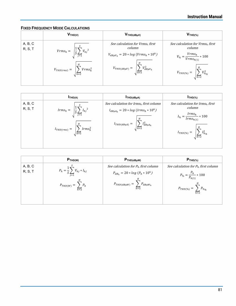
Instruction Manual
81
FIXED FREQUENCY MODE CALCULATIONS
VTHD(V) VTHD(dBµV) VTHD(%)
A, B, C R, S, T 𝑉𝑉𝑎𝑎𝑎𝑎𝑉𝑉ℎ = �
1𝑆𝑆�𝑉𝑉ℎ𝑗𝑗2
𝛴𝛴
𝑗𝑗=1
𝑉𝑉𝛴𝛴𝑇𝑇𝑇𝑇(𝑉𝑉𝑚𝑚𝑉𝑉) = ��𝑉𝑉𝑎𝑎𝑎𝑎𝑉𝑉ℎ2𝑇𝑇
ℎ=2
See calculation for Vrmsh, first column
𝑉𝑉𝑑𝑑𝛴𝛴𝑑𝑑𝑉𝑉ℎ = 20 ∗ 𝐹𝐹𝑎𝑎𝑚𝑚 (𝑉𝑉𝑎𝑎𝑎𝑎𝑉𝑉ℎ ∗ 106)
𝑉𝑉𝛴𝛴𝑇𝑇𝑇𝑇(𝑑𝑑𝛴𝛴𝑑𝑑𝑉𝑉) = ��𝑉𝑉𝑑𝑑𝛴𝛴𝑑𝑑𝑉𝑉ℎ2
𝑇𝑇
ℎ=2
See calculation for Vrmsh, first column
𝑉𝑉% =𝑉𝑉𝑎𝑎𝑎𝑎𝑉𝑉ℎ𝑉𝑉𝑎𝑎𝑎𝑎𝑉𝑉ℎ(1)
∗ 100
𝑉𝑉𝛴𝛴𝑇𝑇𝑇𝑇(%) = ��𝑉𝑉%2ℎ
𝑇𝑇
ℎ=2
ITHD(A) ITHD(dBµA) ITHD(%) A, B, C R, S, T 𝐼𝐼𝑎𝑎𝑎𝑎𝑉𝑉ℎ = �
1𝑆𝑆�𝐼𝐼ℎ𝑗𝑗2
𝛴𝛴
𝑗𝑗=1
𝐼𝐼𝛴𝛴𝑇𝑇𝑇𝑇(𝑉𝑉𝑚𝑚𝑉𝑉) = ��𝐼𝐼𝑎𝑎𝑎𝑎𝑉𝑉ℎ2𝑇𝑇
ℎ=2
See calculation for Irmsh, first column
𝐼𝐼𝑑𝑑𝛴𝛴µ𝛴𝛴ℎ = 20 ∗ 𝐹𝐹𝑎𝑎𝑚𝑚 (𝐼𝐼𝑎𝑎𝑎𝑎𝑉𝑉ℎ ∗ 106)
𝐼𝐼𝛴𝛴𝑇𝑇𝑇𝑇(𝑑𝑑𝛴𝛴µ𝛴𝛴) = ��𝐼𝐼𝑑𝑑𝛴𝛴µ𝛴𝛴ℎ2
𝑇𝑇
ℎ=2
See calculation for Irmsh, first column
𝐼𝐼% =𝐼𝐼𝑎𝑎𝑎𝑎𝑉𝑉ℎ𝐼𝐼𝑎𝑎𝑎𝑎𝑉𝑉ℎ(1)
∗ 100
𝐼𝐼𝛴𝛴𝑇𝑇𝑇𝑇(%) = ��𝐼𝐼%2 ℎ
𝑇𝑇
ℎ=2
PTHD(W) PTHD(dBµW) PTHD(%) A, B, C R, S, T 𝑃𝑃ℎ =
1𝑆𝑆�𝑉𝑉ℎ𝑗𝑗 ∗ 𝐼𝐼ℎ𝑗𝑗
𝛴𝛴
𝑗𝑗=1
𝑃𝑃𝛴𝛴𝑇𝑇𝑇𝑇(𝑊𝑊) = �𝑃𝑃ℎ
𝑇𝑇
ℎ=2
See calculation for Ph, first column
𝑃𝑃𝑑𝑑𝛴𝛴ℎ = 20 ∗ 𝐹𝐹𝑎𝑎𝑚𝑚 (𝑃𝑃ℎ ∗ 106)
𝑃𝑃𝛴𝛴𝑇𝑇𝑇𝑇(𝑑𝑑𝛴𝛴µ𝑊𝑊) = �𝑃𝑃𝑑𝑑𝛴𝛴µ𝑊𝑊ℎ
𝑇𝑇
ℎ=2
See calculation for Ph, first column
𝑃𝑃% =𝑃𝑃ℎ𝑃𝑃ℎ(1)
∗ 100
𝑃𝑃𝛴𝛴𝑇𝑇𝑇𝑇(%) = �𝑃𝑃%ℎ
𝑇𝑇
ℎ=2

3-phase Power Analysis Software
82
THD Measurement Calculations (Numerics Table) THD measurement parameters calculations may yield marginally different results in the Numerics and Harmonics Order tables due to slightly different calculation methods used in each table. The different calculation methods are shown below. While they are different, in both cases the methods meet the standard for calculating THD.
3-PHASE 4-WIRE (3V3A) CALCULATIONS
Vthd Ithd
A,B,C R,S,T 𝑉𝑉𝐹𝐹ℎ𝑜𝑜𝑖𝑖 =
�∑ 𝑉𝑉𝑎𝑎𝑎𝑎𝑉𝑉ℎ𝑖𝑖2𝑇𝑇ℎ=2
𝑉𝑉𝑎𝑎𝑎𝑎𝑉𝑉ℎ(1)𝑖𝑖∗ 100
𝑉𝑉𝐹𝐹ℎ𝑜𝑜 = 1𝑁𝑁�𝑉𝑉𝐹𝐹ℎ𝑜𝑜𝑖𝑖
𝑁𝑁
𝑖𝑖=1
𝐼𝐼𝐹𝐹ℎ𝑜𝑜𝑖𝑖 =�∑ 𝐼𝐼𝑎𝑎𝑎𝑎𝑉𝑉ℎ𝑖𝑖2𝑇𝑇
ℎ=2
𝐼𝐼𝑎𝑎𝑎𝑎𝑉𝑉ℎ(1)𝑖𝑖∗ 100
𝐼𝐼𝐹𝐹ℎ𝑜𝑜 = 1𝑁𝑁�𝐼𝐼𝐹𝐹ℎ𝑜𝑜𝑖𝑖
𝑁𝑁
𝑖𝑖=1
ΣABC 𝑉𝑉𝐹𝐹ℎ𝑜𝑜𝛴𝛴𝛴𝛴𝛴𝛴𝛴𝛴𝑖𝑖 = 13
(𝑉𝑉𝐹𝐹ℎ𝑜𝑜𝛴𝛴𝑖𝑖 + 𝑉𝑉𝐹𝐹ℎ𝑜𝑜𝛴𝛴𝑖𝑖 + 𝑉𝑉𝐹𝐹𝑜𝑜ℎ𝛴𝛴𝑖𝑖)
𝑉𝑉𝐹𝐹ℎ𝑜𝑜𝛴𝛴𝛴𝛴𝛴𝛴𝛴𝛴 = 1𝑁𝑁�𝑉𝑉𝐹𝐹ℎ𝑜𝑜𝛴𝛴𝛴𝛴𝛴𝛴𝛴𝛴𝑖𝑖
𝑁𝑁
𝑖𝑖=1
𝐼𝐼𝐹𝐹ℎ𝑜𝑜𝛴𝛴𝛴𝛴𝛴𝛴𝛴𝛴𝑖𝑖 = 13
(𝐼𝐼𝐹𝐹ℎ𝑜𝑜𝛴𝛴𝑖𝑖 + 𝐼𝐼𝐹𝐹ℎ𝑜𝑜𝛴𝛴𝑖𝑖 + 𝐼𝐼𝐹𝐹ℎ𝑜𝑜𝛴𝛴𝑖𝑖)
𝐼𝐼𝐹𝐹ℎ𝑜𝑜𝛴𝛴𝛴𝛴𝛴𝛴𝛴𝛴 = 1𝑁𝑁�𝐼𝐼𝐹𝐹ℎ𝑜𝑜𝛴𝛴𝛴𝛴𝛴𝛴𝛴𝛴𝑖𝑖
𝑁𝑁
𝑖𝑖=1
ΣRST 𝑉𝑉𝐹𝐹ℎ𝑜𝑜𝛴𝛴𝛴𝛴𝛴𝛴𝛴𝛴𝑖𝑖 = 13
(𝑉𝑉𝐹𝐹ℎ𝑜𝑜𝛴𝛴𝑖𝑖 + 𝑉𝑉𝐹𝐹ℎ𝑜𝑜𝛴𝛴𝑖𝑖 + 𝑉𝑉𝐹𝐹ℎ𝑜𝑜𝛴𝛴𝑖𝑖)
𝑉𝑉𝐹𝐹ℎ𝑜𝑜𝛴𝛴𝛴𝛴𝛴𝛴𝛴𝛴 = 1𝑁𝑁�𝑉𝑉𝐹𝐹ℎ𝑜𝑜𝛴𝛴𝛴𝛴𝛴𝛴𝛴𝛴𝑖𝑖
𝑁𝑁
𝑖𝑖=1
𝐼𝐼𝐹𝐹ℎ𝑜𝑜𝛴𝛴𝛴𝛴𝛴𝛴𝛴𝛴𝑖𝑖 = 13
(𝐼𝐼𝐹𝐹ℎ𝑜𝑜𝛴𝛴𝑖𝑖 + 𝐼𝐼𝐹𝐹ℎ𝑜𝑜𝛴𝛴𝑖𝑖 + 𝐼𝐼𝐹𝐹ℎ𝑜𝑜𝛴𝛴𝑖𝑖)
𝐼𝐼𝐹𝐹ℎ𝑜𝑜𝛴𝛴𝛴𝛴𝛴𝛴𝛴𝛴 = 1𝑁𝑁�𝐼𝐼𝐹𝐹ℎ𝑜𝑜𝛴𝛴𝛴𝛴𝛴𝛴𝛴𝛴𝑖𝑖
𝑁𝑁
𝑖𝑖=1
Pthd
A,B,C R,S,T 𝑃𝑃𝐹𝐹ℎ𝑜𝑜𝑖𝑖 =
∑ 𝑃𝑃ℎ𝑇𝑇ℎ=2
𝑃𝑃𝑎𝑎𝑎𝑎𝑉𝑉ℎ(1)𝑖𝑖∗ 100
𝑃𝑃𝐹𝐹ℎ𝑜𝑜 = 1𝑁𝑁�𝑃𝑃𝐹𝐹ℎ𝑜𝑜𝑖𝑖
𝑁𝑁
𝑖𝑖=1
ΣABC 𝑃𝑃𝐹𝐹ℎ𝑜𝑜𝛴𝛴𝛴𝛴𝛴𝛴𝛴𝛴𝑖𝑖 = 13
(𝑃𝑃𝐹𝐹ℎ𝑜𝑜𝛴𝛴𝑖𝑖 + 𝑃𝑃𝐹𝐹ℎ𝑜𝑜𝛴𝛴𝑖𝑖 + 𝑃𝑃𝐹𝐹𝑜𝑜ℎ𝛴𝛴𝑖𝑖)
𝑃𝑃𝐹𝐹ℎ𝑜𝑜𝛴𝛴𝛴𝛴𝛴𝛴𝛴𝛴 = 1𝑁𝑁�𝑃𝑃𝐹𝐹ℎ𝑜𝑜𝛴𝛴𝛴𝛴𝛴𝛴𝛴𝛴𝑖𝑖
𝑁𝑁
𝑖𝑖=1
ΣRST 𝑃𝑃𝐹𝐹ℎ𝑜𝑜𝛴𝛴𝛴𝛴𝛴𝛴𝛴𝛴𝑖𝑖 = 13
(𝑃𝑃𝐹𝐹ℎ𝑜𝑜𝛴𝛴𝑖𝑖 + 𝑃𝑃𝐹𝐹ℎ𝑜𝑜𝛴𝛴𝑖𝑖 + 𝑃𝑃𝐹𝐹ℎ𝑜𝑜𝛴𝛴𝑖𝑖)
𝑃𝑃𝐹𝐹ℎ𝑜𝑜𝛴𝛴𝛴𝛴𝛴𝛴𝛴𝛴 = 1𝑁𝑁�𝑃𝑃𝐹𝐹ℎ𝑜𝑜𝛴𝛴𝛴𝛴𝛴𝛴𝛴𝛴𝑖𝑖
𝑁𝑁
𝑖𝑖=1

Instruction Manual
83
3-PHASE 3-WIRE (3V3A) CALCULATIONS
Vthd Ithd
Voltage: AB,BC,CA RS,ST,TR Current: A, B, C R, S, T
𝑉𝑉𝐹𝐹ℎ𝑜𝑜𝑖𝑖 =�∑ 𝑉𝑉𝑎𝑎𝑎𝑎𝑉𝑉ℎ𝑖𝑖2𝑇𝑇
ℎ=2
𝑉𝑉𝑎𝑎𝑎𝑎𝑉𝑉ℎ(1)𝑖𝑖∗ 100
𝑉𝑉𝐹𝐹ℎ𝑜𝑜 = 1𝑁𝑁�𝑉𝑉𝐹𝐹ℎ𝑜𝑜𝑖𝑖
𝑁𝑁
𝑖𝑖=1
𝐼𝐼𝐹𝐹ℎ𝑜𝑜𝑖𝑖 =�∑ 𝐼𝐼𝑎𝑎𝑎𝑎𝑉𝑉ℎ𝑖𝑖2𝑇𝑇
ℎ=2
𝐼𝐼𝑎𝑎𝑎𝑎𝑉𝑉ℎ(1)𝑖𝑖∗ 100
𝐼𝐼𝐹𝐹ℎ𝑜𝑜 = 1𝑁𝑁�𝐼𝐼𝐹𝐹ℎ𝑜𝑜𝑖𝑖
𝑁𝑁
𝑖𝑖=1
ΣABC 𝑉𝑉𝐹𝐹ℎ𝑜𝑜𝛴𝛴𝛴𝛴𝛴𝛴𝛴𝛴𝑖𝑖 = 13
(𝑉𝑉𝐹𝐹ℎ𝑜𝑜𝛴𝛴𝛴𝛴𝑖𝑖 + 𝑉𝑉𝐹𝐹ℎ𝑜𝑜𝛴𝛴𝛴𝛴𝑖𝑖 + 𝑉𝑉𝐹𝐹𝑜𝑜ℎ𝛴𝛴𝛴𝛴𝑖𝑖)
𝑉𝑉𝐹𝐹ℎ𝑜𝑜𝛴𝛴𝛴𝛴𝛴𝛴𝛴𝛴 = 1𝑁𝑁�𝑉𝑉𝐹𝐹ℎ𝑜𝑜𝛴𝛴𝛴𝛴𝛴𝛴𝛴𝛴𝑖𝑖
𝑁𝑁
𝑖𝑖=1
𝐼𝐼𝐹𝐹ℎ𝑜𝑜𝛴𝛴𝛴𝛴𝛴𝛴𝛴𝛴𝑖𝑖 = 13
(𝐼𝐼𝐹𝐹ℎ𝑜𝑜𝛴𝛴𝛴𝛴𝑖𝑖 + 𝐼𝐼𝐹𝐹ℎ𝑜𝑜𝛴𝛴𝛴𝛴𝑖𝑖 + 𝐼𝐼𝐹𝐹ℎ𝑜𝑜𝛴𝛴𝛴𝛴𝑖𝑖)
𝐼𝐼𝐹𝐹ℎ𝑜𝑜𝛴𝛴𝛴𝛴𝛴𝛴𝛴𝛴 = 1𝑁𝑁�𝐼𝐼𝐹𝐹ℎ𝑜𝑜𝛴𝛴𝛴𝛴𝛴𝛴𝛴𝛴𝑖𝑖
𝑁𝑁
𝑖𝑖=1
ΣRST 𝑉𝑉𝐹𝐹ℎ𝑜𝑜𝛴𝛴𝛴𝛴𝛴𝛴𝛴𝛴𝑖𝑖 = 13
(𝑉𝑉𝐹𝐹ℎ𝑜𝑜𝛴𝛴𝛴𝛴𝑖𝑖 + 𝑉𝑉𝐹𝐹ℎ𝑜𝑜𝛴𝛴𝛴𝛴𝑖𝑖 + 𝑉𝑉𝐹𝐹ℎ𝑜𝑜𝛴𝛴𝛴𝛴𝑖𝑖)
𝑉𝑉𝐹𝐹ℎ𝑜𝑜𝛴𝛴𝛴𝛴𝛴𝛴𝛴𝛴 = 1𝑁𝑁�𝑉𝑉𝐹𝐹ℎ𝑜𝑜𝛴𝛴𝛴𝛴𝛴𝛴𝛴𝛴𝑖𝑖
𝑁𝑁
𝑖𝑖=1
𝐼𝐼𝐹𝐹ℎ𝑜𝑜𝛴𝛴𝛴𝛴𝛴𝛴𝛴𝛴𝑖𝑖 = 13
(𝐼𝐼𝐹𝐹ℎ𝑜𝑜𝛴𝛴𝑖𝑖 + 𝐼𝐼𝐹𝐹ℎ𝑜𝑜𝛴𝛴𝑖𝑖 + 𝐼𝐼𝐹𝐹ℎ𝑜𝑜𝛴𝛴𝑖𝑖)
𝐼𝐼𝐹𝐹ℎ𝑜𝑜𝛴𝛴𝛴𝛴𝛴𝛴𝛴𝛴 = 1𝑁𝑁�𝐼𝐼𝐹𝐹ℎ𝑜𝑜𝛴𝛴𝛴𝛴𝛴𝛴𝛴𝛴𝑖𝑖
𝑁𝑁
𝑖𝑖=1
Pthd
Voltage: AB,BC,CA RS,ST,TR Current: A, B, C R, S, T
𝑃𝑃𝐹𝐹ℎ𝑜𝑜𝑖𝑖 =∑ 𝑃𝑃ℎ𝑇𝑇ℎ=2
𝑃𝑃𝑎𝑎𝑎𝑎𝑉𝑉ℎ(1)𝑖𝑖∗ 100
𝑃𝑃𝐹𝐹ℎ𝑜𝑜 = 1𝑁𝑁�𝑃𝑃𝐹𝐹ℎ𝑜𝑜𝑖𝑖
𝑁𝑁
𝑖𝑖=1
ΣABC 𝑃𝑃𝐹𝐹ℎ𝑜𝑜𝛴𝛴𝛴𝛴𝛴𝛴𝛴𝛴𝑖𝑖 = 13
(𝑃𝑃𝐹𝐹ℎ𝑜𝑜𝛴𝛴𝛴𝛴𝑖𝑖 + 𝑃𝑃𝐹𝐹ℎ𝑜𝑜𝛴𝛴𝛴𝛴𝑖𝑖 + 𝑃𝑃𝐹𝐹𝑜𝑜ℎ𝛴𝛴𝛴𝛴𝑖𝑖)
𝑃𝑃𝐹𝐹ℎ𝑜𝑜𝛴𝛴𝛴𝛴𝛴𝛴𝛴𝛴 = 1𝑁𝑁�𝑃𝑃𝐹𝐹ℎ𝑜𝑜𝛴𝛴𝛴𝛴𝛴𝛴𝛴𝛴𝑖𝑖
𝑁𝑁
𝑖𝑖=1
ΣRST 𝑃𝑃𝐹𝐹ℎ𝑜𝑜𝛴𝛴𝛴𝛴𝛴𝛴𝛴𝛴𝑖𝑖 = 13
(𝑃𝑃𝐹𝐹ℎ𝑜𝑜𝛴𝛴𝛴𝛴𝑖𝑖 + 𝑃𝑃𝐹𝐹ℎ𝑜𝑜𝛴𝛴𝛴𝛴𝑖𝑖 + 𝑃𝑃𝐹𝐹ℎ𝑜𝑜𝛴𝛴𝛴𝛴𝑖𝑖)
𝑃𝑃𝐹𝐹ℎ𝑜𝑜𝛴𝛴𝛴𝛴𝛴𝛴𝛴𝛴 = 1𝑁𝑁�𝑃𝑃𝐹𝐹ℎ𝑜𝑜𝛴𝛴𝛴𝛴𝛴𝛴𝛴𝛴𝑖𝑖
𝑁𝑁
𝑖𝑖=1
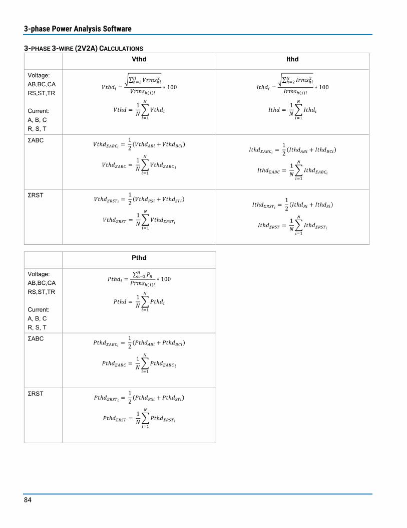
3-phase Power Analysis Software
84
3-PHASE 3-WIRE (2V2A) CALCULATIONS
Vthd Ithd
Voltage: AB,BC,CA RS,ST,TR Current: A, B, C R, S, T
𝑉𝑉𝐹𝐹ℎ𝑜𝑜𝑖𝑖 =�∑ 𝑉𝑉𝑎𝑎𝑎𝑎𝑉𝑉ℎ𝑖𝑖2𝑇𝑇
ℎ=2
𝑉𝑉𝑎𝑎𝑎𝑎𝑉𝑉ℎ(1)𝑖𝑖∗ 100
𝑉𝑉𝐹𝐹ℎ𝑜𝑜 = 1𝑁𝑁�𝑉𝑉𝐹𝐹ℎ𝑜𝑜𝑖𝑖
𝑁𝑁
𝑖𝑖=1
𝐼𝐼𝐹𝐹ℎ𝑜𝑜𝑖𝑖 =�∑ 𝐼𝐼𝑎𝑎𝑎𝑎𝑉𝑉ℎ𝑖𝑖2𝑇𝑇
ℎ=2
𝐼𝐼𝑎𝑎𝑎𝑎𝑉𝑉ℎ(1)𝑖𝑖∗ 100
𝐼𝐼𝐹𝐹ℎ𝑜𝑜 = 1𝑁𝑁�𝐼𝐼𝐹𝐹ℎ𝑜𝑜𝑖𝑖
𝑁𝑁
𝑖𝑖=1
ΣABC 𝑉𝑉𝐹𝐹ℎ𝑜𝑜𝛴𝛴𝛴𝛴𝛴𝛴𝛴𝛴𝑖𝑖 = 12
(𝑉𝑉𝐹𝐹ℎ𝑜𝑜𝛴𝛴𝛴𝛴𝑖𝑖 + 𝑉𝑉𝐹𝐹ℎ𝑜𝑜𝛴𝛴𝛴𝛴𝑖𝑖)
𝑉𝑉𝐹𝐹ℎ𝑜𝑜𝛴𝛴𝛴𝛴𝛴𝛴𝛴𝛴 = 1𝑁𝑁�𝑉𝑉𝐹𝐹ℎ𝑜𝑜𝛴𝛴𝛴𝛴𝛴𝛴𝛴𝛴𝑖𝑖
𝑁𝑁
𝑖𝑖=1
𝐼𝐼𝐹𝐹ℎ𝑜𝑜𝛴𝛴𝛴𝛴𝛴𝛴𝛴𝛴𝑖𝑖 = 12
(𝐼𝐼𝐹𝐹ℎ𝑜𝑜𝛴𝛴𝛴𝛴𝑖𝑖 + 𝐼𝐼𝐹𝐹ℎ𝑜𝑜𝛴𝛴𝛴𝛴𝑖𝑖)
𝐼𝐼𝐹𝐹ℎ𝑜𝑜𝛴𝛴𝛴𝛴𝛴𝛴𝛴𝛴 = 1𝑁𝑁�𝐼𝐼𝐹𝐹ℎ𝑜𝑜𝛴𝛴𝛴𝛴𝛴𝛴𝛴𝛴𝑖𝑖
𝑁𝑁
𝑖𝑖=1
ΣRST 𝑉𝑉𝐹𝐹ℎ𝑜𝑜𝛴𝛴𝛴𝛴𝛴𝛴𝛴𝛴𝑖𝑖 = 12
(𝑉𝑉𝐹𝐹ℎ𝑜𝑜𝛴𝛴𝛴𝛴𝑖𝑖 + 𝑉𝑉𝐹𝐹ℎ𝑜𝑜𝛴𝛴𝛴𝛴𝑖𝑖)
𝑉𝑉𝐹𝐹ℎ𝑜𝑜𝛴𝛴𝛴𝛴𝛴𝛴𝛴𝛴 = 1𝑁𝑁�𝑉𝑉𝐹𝐹ℎ𝑜𝑜𝛴𝛴𝛴𝛴𝛴𝛴𝛴𝛴𝑖𝑖
𝑁𝑁
𝑖𝑖=1
𝐼𝐼𝐹𝐹ℎ𝑜𝑜𝛴𝛴𝛴𝛴𝛴𝛴𝛴𝛴𝑖𝑖 = 12
(𝐼𝐼𝐹𝐹ℎ𝑜𝑜𝛴𝛴𝑖𝑖 + 𝐼𝐼𝐹𝐹ℎ𝑜𝑜𝛴𝛴𝑖𝑖)
𝐼𝐼𝐹𝐹ℎ𝑜𝑜𝛴𝛴𝛴𝛴𝛴𝛴𝛴𝛴 = 1𝑁𝑁�𝐼𝐼𝐹𝐹ℎ𝑜𝑜𝛴𝛴𝛴𝛴𝛴𝛴𝛴𝛴𝑖𝑖
𝑁𝑁
𝑖𝑖=1
Pthd
Voltage: AB,BC,CA RS,ST,TR Current: A, B, C R, S, T
𝑃𝑃𝐹𝐹ℎ𝑜𝑜𝑖𝑖 =∑ 𝑃𝑃ℎ𝑇𝑇ℎ=2
𝑃𝑃𝑎𝑎𝑎𝑎𝑉𝑉ℎ(1)𝑖𝑖∗ 100
𝑃𝑃𝐹𝐹ℎ𝑜𝑜 = 1𝑁𝑁�𝑃𝑃𝐹𝐹ℎ𝑜𝑜𝑖𝑖
𝑁𝑁
𝑖𝑖=1
ΣABC 𝑃𝑃𝐹𝐹ℎ𝑜𝑜𝛴𝛴𝛴𝛴𝛴𝛴𝛴𝛴𝑖𝑖 = 12
(𝑃𝑃𝐹𝐹ℎ𝑜𝑜𝛴𝛴𝛴𝛴𝑖𝑖 + 𝑃𝑃𝐹𝐹ℎ𝑜𝑜𝛴𝛴𝛴𝛴𝑖𝑖)
𝑃𝑃𝐹𝐹ℎ𝑜𝑜𝛴𝛴𝛴𝛴𝛴𝛴𝛴𝛴 = 1𝑁𝑁�𝑃𝑃𝐹𝐹ℎ𝑜𝑜𝛴𝛴𝛴𝛴𝛴𝛴𝛴𝛴𝑖𝑖
𝑁𝑁
𝑖𝑖=1
ΣRST 𝑃𝑃𝐹𝐹ℎ𝑜𝑜𝛴𝛴𝛴𝛴𝛴𝛴𝛴𝛴𝑖𝑖 = 12
(𝑃𝑃𝐹𝐹ℎ𝑜𝑜𝛴𝛴𝛴𝛴𝑖𝑖 + 𝑃𝑃𝐹𝐹ℎ𝑜𝑜𝛴𝛴𝛴𝛴𝑖𝑖)
𝑃𝑃𝐹𝐹ℎ𝑜𝑜𝛴𝛴𝛴𝛴𝛴𝛴𝛴𝛴 = 1𝑁𝑁�𝑃𝑃𝐹𝐹ℎ𝑜𝑜𝛴𝛴𝛴𝛴𝛴𝛴𝛴𝛴𝑖𝑖
𝑁𝑁
𝑖𝑖=1

Instruction Manual
85
1-PHASE/3-WIRE (2 VOLTAGE AND 2 CURRENT) CALCULATIONS
Vthd Ithd
A, B 𝑉𝑉𝐹𝐹ℎ𝑜𝑜𝑖𝑖 =
�∑ 𝑉𝑉𝑎𝑎𝑎𝑎𝑉𝑉ℎ𝑖𝑖2𝑇𝑇ℎ=2
𝑉𝑉𝑎𝑎𝑎𝑎𝑉𝑉ℎ(1)𝑖𝑖∗ 100
𝑉𝑉𝐹𝐹ℎ𝑜𝑜 = 1𝑁𝑁�𝑉𝑉𝐹𝐹ℎ𝑜𝑜𝑖𝑖
𝑁𝑁
𝑖𝑖=1
𝐼𝐼𝐹𝐹ℎ𝑜𝑜𝑖𝑖 =�∑ 𝐼𝐼𝑎𝑎𝑎𝑎𝑉𝑉ℎ𝑖𝑖2𝑇𝑇
ℎ=2
𝐼𝐼𝑎𝑎𝑎𝑎𝑉𝑉ℎ(1)𝑖𝑖∗ 100
𝐼𝐼𝐹𝐹ℎ𝑜𝑜 = 1𝑁𝑁�𝐼𝐼𝐹𝐹ℎ𝑜𝑜𝑖𝑖
𝑁𝑁
𝑖𝑖=1
ΣAB 𝑉𝑉𝐹𝐹ℎ𝑜𝑜𝛴𝛴𝛴𝛴𝛴𝛴𝛴𝛴𝑖𝑖 = 12
(𝑉𝑉𝐹𝐹ℎ𝑜𝑜𝛴𝛴𝑖𝑖 + 𝑉𝑉𝐹𝐹ℎ𝑜𝑜𝛴𝛴𝑖𝑖)
𝑉𝑉𝐹𝐹ℎ𝑜𝑜𝛴𝛴𝛴𝛴𝛴𝛴𝛴𝛴 = 1𝑁𝑁�𝑉𝑉𝐹𝐹ℎ𝑜𝑜𝛴𝛴𝛴𝛴𝛴𝛴𝛴𝛴𝑖𝑖
𝑁𝑁
𝑖𝑖=1
𝐼𝐼𝐹𝐹ℎ𝑜𝑜𝛴𝛴𝛴𝛴𝛴𝛴𝛴𝛴𝑖𝑖 = 12
(𝐼𝐼𝐹𝐹ℎ𝑜𝑜𝛴𝛴𝑖𝑖 + 𝐼𝐼𝐹𝐹ℎ𝑜𝑜𝛴𝛴𝑖𝑖)
𝐼𝐼𝐹𝐹ℎ𝑜𝑜𝛴𝛴𝛴𝛴𝛴𝛴𝛴𝛴 = 1𝑁𝑁�𝐼𝐼𝐹𝐹ℎ𝑜𝑜𝛴𝛴𝛴𝛴𝛴𝛴𝛴𝛴𝑖𝑖
𝑁𝑁
𝑖𝑖=1
Pthd
Voltage: AB,BC,CA RS,ST,TR Current: A, B, C R, S, T
𝑃𝑃𝐹𝐹ℎ𝑜𝑜𝑖𝑖 =∑ 𝑃𝑃ℎ𝑇𝑇ℎ=2
𝑃𝑃𝑎𝑎𝑎𝑎𝑉𝑉ℎ(1)𝑖𝑖∗ 100
𝑃𝑃𝐹𝐹ℎ𝑜𝑜 = 1𝑁𝑁�𝑃𝑃𝐹𝐹ℎ𝑜𝑜𝑖𝑖
𝑁𝑁
𝑖𝑖=1
ΣABC 𝑃𝑃𝐹𝐹ℎ𝑜𝑜𝛴𝛴𝛴𝛴𝛴𝛴𝛴𝛴𝑖𝑖 = 12
(𝑃𝑃𝐹𝐹ℎ𝑜𝑜𝛴𝛴𝑖𝑖 + 𝑃𝑃𝐹𝐹ℎ𝑜𝑜𝛴𝛴𝑖𝑖)
𝑃𝑃𝐹𝐹ℎ𝑜𝑜𝛴𝛴𝛴𝛴𝛴𝛴𝛴𝛴 = 1𝑁𝑁�𝑃𝑃𝐹𝐹ℎ𝑜𝑜𝛴𝛴𝛴𝛴𝛴𝛴𝛴𝛴𝑖𝑖
𝑁𝑁
𝑖𝑖=1
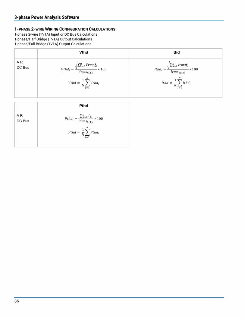
3-phase Power Analysis Software
86
1-PHASE 2-WIRE WIRING CONFIGURATION CALCULATIONS 1-phase 2-wire (1V1A) Input or DC Bus Calculations 1-phase/Half-Bridge (1V1A) Output Calculations 1-phase/Full-Bridge (1V1A) Output Calculations
Vthd Ithd
A R DC Bus 𝑉𝑉𝐹𝐹ℎ𝑜𝑜𝑖𝑖 =
�∑ 𝑉𝑉𝑎𝑎𝑎𝑎𝑉𝑉ℎ𝑖𝑖2𝑇𝑇ℎ=2
𝑉𝑉𝑎𝑎𝑎𝑎𝑉𝑉ℎ(1)𝑖𝑖∗ 100
𝑉𝑉𝐹𝐹ℎ𝑜𝑜 = 1𝑁𝑁�𝑉𝑉𝐹𝐹ℎ𝑜𝑜𝑖𝑖
𝑁𝑁
𝑖𝑖=1
𝐼𝐼𝐹𝐹ℎ𝑜𝑜𝑖𝑖 =�∑ 𝐼𝐼𝑎𝑎𝑎𝑎𝑉𝑉ℎ𝑖𝑖2𝑇𝑇
ℎ=2
𝐼𝐼𝑎𝑎𝑎𝑎𝑉𝑉ℎ(1)𝑖𝑖∗ 100
𝐼𝐼𝐹𝐹ℎ𝑜𝑜 = 1𝑁𝑁�𝐼𝐼𝐹𝐹ℎ𝑜𝑜𝑖𝑖
𝑁𝑁
𝑖𝑖=1
Pthd
A R DC Bus 𝑃𝑃𝐹𝐹ℎ𝑜𝑜𝑖𝑖 =
∑ 𝑃𝑃ℎ𝑇𝑇ℎ=2
𝑃𝑃𝑎𝑎𝑎𝑎𝑉𝑉ℎ(1)𝑖𝑖∗ 100
𝑃𝑃𝐹𝐹ℎ𝑜𝑜 = 1𝑁𝑁�𝑃𝑃𝐹𝐹ℎ𝑜𝑜𝑖𝑖
𝑁𝑁
𝑖𝑖=1