Types of bonds 1. Metallic Solids 2. Ionic Solids 3. Molecular Solids 4. Covalent network solids.
3 Methods for Band Structure Calculationsin Solids
A. Ernst1 and M. Luders2
1 Max-Planck-Institut fur Mikrostrukturphysik, Weinberg 2, 06120 Halle,Germany
2 Daresbury Laboratory, Warrington WA4 4AD, United Kingdom
Abstract. The calculation of the ground-state and excited-state properties of ma-terials is one of the main goals of condensed matter physics. While the most suc-cessful first-principles method, the density-functional theory (DFT), provides, inprinciple, the exact ground-state properties, the many-body method is the mostsuitable approach for studying excited-state properties of extended systems. Herewe discuss general aspects of the Green’s function and different approximations forthe self-energy to solve the Dyson equation. Further we present some tools for solv-ing the Dyson equation with several approximations for the self-energy: a highlyprecise combined basis method providing the band structure in the Kohn-Shamapproximation, and some implementations for the random-phase approximation.
3.1 The Green’s Function and the Many-Body Method
3.1.1 General Considerations
The Green’s function is a powerful tool for studying ground state and excitedstate properties of condensed matter. The basic idea of the Green’s functionhas its origin in the theory of differential equations. The solution of anyinhomogeneous differential equation with a Hermitian differential operatorH, a complex parameter z, and a given source function u(r) of the form[
z − H(r)]ψ(r) = u(r) (3.1)
can be represented as an integral equation
ψ(r) = ϕ(r) +∫
G(r, r′; z)u(r′)d3r′. (3.2)
Here the so-called Green’s function G(r, r′; z) is a coordinate representationof the resolvent of the differential operator H, i.e. G = [z−H]−1, which obeysthe differential equation[
z − H(r)]G(r, r′; z) = δ(r − r′), (3.3)
and the function ϕ(r) is a general solution of the homogeneous equation as-sociated with (3.1), i.e. for u(r) = 0. The integral equation (3.2) contains, in
A. Ernst and M. Luders, Methods for Band Structure Calculations in Solids, Lect. Notes Phys.642, 23–54 (2004)http://www.springerlink.com/ c© Springer-Verlag Berlin Heidelberg 2004

24 A. Ernst and M. Luders
contrast to the differential equation (3.1), also information about the bound-ary conditions, which are built into the function ϕ(r). This method is inmany cases very convenient and widely used in many-body physics. In thisreview we shall consider the application of the Green’s function method incondensed matter physics at zero temperature. The formalism can be gener-alised to finite temperatures but this is beyond the scope of this papers andcan be found in standard textbooks [3.22,3.42,3.24]
The evolution of an N -body system is determined by the time-dependentSchrodinger equation (atomic units are used throughout)
idΨ(t)dt
= HΨ(t), (3.4)
where Ψ(t) ≡ Ψ(r1, r2, ..., rN ; t) is a wave function of the system and H isthe many-body Hamiltonian
H = H0 + V , (3.5)
which includes the kinetic energy and the external potential
H0 = −∑
i
∇2i
2+∑
i
vext(ri), (3.6)
and the interactions between the particles
V =12
∑i,j
1|ri − rj |
. (3.7)
Knowing the wave function Ψ(t), the average value of any operator A can beobtained from the equation:
A(t) = 〈Ψ∗(t)AΨ(t)〉 . (3.8)
The many-body wave function can be expanded in a complete set of time-independent either anti-symmetrized (for fermions) or symmetrized (forbosons) products of single particle wave-functions: Φi1,...,in(r1, . . . , rN )
Ψ(r1, r2, ..rN ; t) =∑
i1,i2,...,iNCi1,i2,...,iN(t)Φi1,...,in(r1, . . . , rN ). (3.9)
These (anti-) symmetrized products of single-particle states φi(r) are givenby
Φi1,...,in(r1, . . . , rN ) =
∑P
(±1)PφP(i1)(r1)φP(i2)(r2)...φP(iN )(rN ) (3.10)
where P denotes all permutations of the indices i1, . . . , iN and (−1)P yields aminus sign for odd permutations. In case of Fermions this anti-symmetrized

3 Methods for Band Structure Calculations in Solids 25
product can conveniently be written as a determinant, the so-called Slaterdeterminant,
Φi1,...,in(r1, . . . , rN ) = |φi1(r1), φi2(r2), . . . φiN(rN )|, (3.11)
which already fulfills Pauli’s exclusion principle. The basis set can be arbi-trary, but in practice one uses functions which are adequate for the particlarproblem. For example, the plane wave basis is appropriate for the descriptionof a system with free or nearly free electrons. Systems with localised electronsare usually better described by atomic-like functions. For systems with a largenumber of particles solving equation (3.4) using the basis expansion (3.9) isa quite formidable task.
To describe a many-body system one can use the so-called second quanti-sation: instead of giving a complete wave function one specifies the numbersof particles to be found in the one-particle states φ1(r), φ2(r), .., φN (r). As aresult the many-body wave function is defined by the expansion coefficients atthe occupation numbers and the Hamiltonian, as well as any other operatorcan be expressed in terms of the so-called creation and annihilation opera-tors c+i and ci, obeying certain commutation or anticommutation relationsaccording to the statistical properties of the particles (fermions or bosons).The creation operator c+i increases the number of particles by one, while theannihilation operators ci decreases the occupation number of a state by one.Any observable can be represented as some combination of these operators.For example, a one-particle operator A can be expressed as
A =∑i,k
Aik c+i ck, (3.12)
where Aik are matrix elements of A. Often it is convenient to use the fieldoperators 1
ψ+σ (r) =
∑i
φiσ(r)c+iσ
ψσ(r) =∑
i
φiσ(r)ciσ , (3.13)
which can be interpreted as creation and annihilation operators of a particlewith spin σ at a given point r. In this representation a single particle operatoris given as
A =∑
σ
∫d3rψ+
σ (r)Aψσ(r), (3.14)
1 Here we have explicitly included the spin-indices. In the remainder of the pa-per, we include the spin in the other quantum numbers, wherever not specifiedexplicitly

26 A. Ernst and M. Luders
where A is of the same form as the operator A in first quantisation, butwithout coordinates and momenta beeing operators.
Suppose we have a system with N particles in the ground state, whichis defined by the exact ground state wave function Ψ0. If at time t0 = 0a particle with quantum number i is added into the system, the systemis described by c+i |Ψ0〉. The evolution of the system in time will now pro-ceed according to e−iH(t−t0)c+i |Ψ0〉. The probability amplitude for findingthe added particle in the state j, is the scalar product of e−iH(t−t0)c+i |Ψ0〉with the function c+j e
−iH(t−t0)|Ψ0〉, describing a particle in the state j, addedto the ground state at time t. The resulting probability amplitude is givenby 〈Ψ0|eiH(t−t0)cje
−iH(t−t0)c+i |Ψ0〉. Analogously, a particle removed from astate can be described with the function ±〈Ψ0|e−iH(t−t0)c+i e
iH(t−t0)cj |Ψ0〉,where plus sign applies to Bose statistics and minus sign to Fermi statistics.Both processes contribute to the definition of the one-particle causal Green’sfunction:
G(j, t; i, t0) = −i〈Ψ0|T[cj(t)c+i (t0)
]|Ψ0〉. (3.15)
Here we have used Heisenberg representation of the operators ci and c+i :
ci(t) = eiHtcie−iHt . (3.16)
The symbol T (3.15) is Wick’s time-ordering operator which rearranges aproduct of two time-dependent operators so that the operator referring tothe later time appears always on the left:
T[cj(t)c+i (t0)
]=
cj(t)c+i (t0) (t > t0)±c+i (t0)cj(t) (t < t0)
. (3.17)
The physical meaning of the Green’s function in this representation is thatfor t > t0 G(i, t0; j, t) describes the propagation of a particle created at timet0 in the state i and detected at time t in the state j. For t < t0, the Green’sfunction describes the propagation of a hole in the state j emitted at time tinto the state i at time t0. Analogously to the above, one can write down theGreen’s function in the space-time representation:
G(r0, t0; r, t) = −i〈Ψ0|T[ψ(r0, t0)ψ+(r, t)
]|Ψ0〉, (3.18)
where ψ(r, t) and ψ+(r, t) are particle annihilation and creation operators inthe Heisenberg representation.
The time-evolution of the Green’s function is controlled by the equationof motion. For V = 0 this is reduced to(
i∂
∂t− H(r)
)G(rt, r′t′) = δ(r − r′)δ(t− t′), (3.19)

3 Methods for Band Structure Calculations in Solids 27
which follows directly from the equation of motion of the field operators:
i∂ψ(r, t)
∂t=[ψ(r, t), H
], (3.20)
and a similar equation for the creation operator ψ+(r, t). Taking the Fouriertransform of (3.19) into frequency space, we get
[ω − H(r)
]G(r, r′;ω) = δ(r − r′), (3.21)
which demonstrates, that G(r, r′;ω) is a Green’s function in the mathemat-ical sence, as described above in (3.3).
The one-particle Green’s function has some important properties whichmake the use of the Green’s function method in condensed matter physicsattractive. The Green’s function contains a great deal of information aboutthe system: knowing the single-particle Green’s function, one can calculatethe ground state expectation value of any single-particle operator:
A(t) = ±i∫ [
limt′→t+0
limr′→r
A(r)G(r, t; r′, t′)]d3r. (3.22)
As a consequence, in particular, the charge density and the total energy canbe found for any system in the ground state at zero temperature. Furthermorethe one-particle Green’s function describes single-particle excitations. In whatfollows, we shall discuss the latter in more detail.
For simplicity, in the following paragraphs we consider the homogeneouselectron gas. Due to the translational invariance, the momentum k is a goodquantum number, and we can use the basis functions φk(r) = 1√
Neik·r. It
can easily be verified that the Green’s function of the homogeneous electrongas is diagonal in momentum space and depends only on the time difference:
G(kt,k′t′) = δk,k′G(k, t− t′) (3.23)
The time-ordering operator T can be mathematically expressed using theHeaviside function θ(t), which leads to the following equation for the Green’sfunction
iGk(t− t′) = θ(t− t′)∑
n
e−i[EN+1n −EN
0 ](t−t′)|〈N + 1, n|c+k |N, 0〉|2
±θ(t′ − t)∑
n
e−i[EN0 −EN−1
n ](t−t′)|〈N − 1, n|ck|N, 0〉|2 . (3.24)
Here EN+1n and EN−1
n are all the exact eigenvalues of the N + 1 and N − 1particle systems respectively, n represents all quantum numbers necessary tospecify the state completely, and EN
0 is the exact ground state energy for thesystem with N particles (n = 0). Using the integral form of the Heavisidefunction,

28 A. Ernst and M. Luders
θ(t) = − limΓ→0
12πi
∞∫−∞
e−iωt
ω + iΓ, (3.25)
the Green’s function can easily be Fourier transformed into the frequencyrepresentation:
Gk(ω) = limΓ→0
[∑n
|〈N + 1, n|c+k |N, 0〉|2
ω −[EN+1
n − EN0
]+ iΓ
∓∑
n
|〈N − 1, n|ck|N, 0〉|2
ω −[EN
0 − EN−1n
]− iΓ
]. (3.26)
Equation (3.26) provides insight into the analytical properties of the single-particle Green’s function. The frequency ω appears only in the denominatorsof the above equation. The Green’s function is a meromorphic function ofthe complex variable ω, and all its singularities are simple poles, which areinfinitesimally shifted into the upper half-plane of ω when ω > 0 and into thelower one if ω < 0. Each pole corresponds to an excitation energy. If we nowset
EN+1n − EN
0 = (EN+1n − EN+1
0 ) + (EN+10 − EN
0 ) = ωn − µ
EN−1n − EN
0 = (EN−1n − EN−1
0 ) + (EN−10 − EN
0 ) = µ′ − ω′n, (3.27)
then ωn and ω′n denote excitation energies in the (N + 1)-and (N − 1)-particle systems respectively and µ and µ′ are changes of the ground stateenergy when a particle is added to the N -particle system or otherwise isremoved from the N -particle system, , known as the chemical potentials. Inthe thermodynamic limit (N → ∞, V → ∞, N/V = const) one finds withinan error of the order N−1 that the chemical potential and the excitationenergies are independent of the particle number, i.e.
ωn ≈ ω′n , µ ≈ µ′ .
Another simple property of the Green’s function which follows from (3.26) isthe asymptotic behaviour for large |ω|:
Gk(ω) ∼ 1ω. (3.28)
It is convenient to introduce the spectral densities:
A+k (ε) =
∑n
|〈N + 1, n|c+k |N, 0〉|2δ(ε− ωn) (3.29 a)
A−k (ε) =∑
n
|〈N − 1, n|ck|N, 0〉|2δ(ε− ωn), (3.29 b)
3 Methods for Band Structure Calculations in Solids 29
which are real and positive functions, and whose physical interpretation issimple. The spectral density function A+
k (ω) gives the probability that theoriginal N -particle system with a particle added into the state k will befound in an exact eigenstate of the (N+1)-particle system. In other words, itcounts the number of states with excitation energy ω and momentum k whichare connected to the ground state through the addition of an extra particle.Similarly, the function A−k (ω) is the probability that the original N -particlesystem and a hole will be found at an exact eigenstate of the (N −1)-particlesystem. Using the spectral functions (3.29), we may write the causal Green’sfunction (3.26) in the Lehmann representation:
Gk(ω) = limΓ→0
∞∫0
dε
[A+
k (ε)ω − (ε+ µ) + iΓ
∓∑
n
A−k (ε)ω + ε− µ− iΓ
]. (3.30)
In addition, the spectral functions (3.29) may by expressed via the causalGreen’s function (3.26):
A+k (ω − µ) = − 1
πImGk(ω), ω > µ (3.31 a)
A−k (µ− ω) = ± 1π
ImGk(ω), ω < µ (3.31 b)
3.1.2 Quasi-Particles
From the Lehmann representation of the Green’s function (3.30), it easy to seethat the special features of the Green’s function originate from the denomina-tor whose zeros can be interpreted as single-particle excitations. If the Green’sfunction has a pole ωk in the momentum state k, then the spectral functionA+
k (ω) will have a strong maximum at the energy ωk = ω − µ. If c+k |N〉 wasan eigenstate, the peak would be a δ-function. In the presence of an interac-tion, the state c+k |N〉 will not be, in general, an eigenstate. The system willhave many other states with the same momentum. An exact eigenstate willbe a linear combination of the respective Slater determinants with energiesspread out by the interaction. The shape of the function A+
k (ω) will dependstrongly on the interaction: the stronger the interaction the larger the spreadof energies and hence the larger the width of the function A+
k (ω). Insertingthe spectral functions back into the time-representation of the Green’s func-tion, one sees that a finite width of the spectral function gives rise to a loss ofcoherence with increasing time, and hence to a damping of the propagation.The behaviour for positive times will be approximately:
iGk(t) ∼ zke−iωkt−Γkt + iGincoherent
k (t), Γk > 0, t > 0 (3.32)
30 A. Ernst and M. Luders
where ωk defines the quasi-particle energy, Γk the quasi-particle inverse life-time. The factor zk is called the quasi-particle weight and describes theamount of coherence in the quasi-particle Green’s function.
The above quasi-particle Green’s function reads in frequency space:
Gk(ω) =zk
ω − ωk + iΓk+Gincoherent
k (ω), ω > µ, (3.33)
Now, in contrast to (3.26), Γk is finite because it is determined by the inter-actions. The incoherent part of the Green’s function is a smooth and mainlystructureless function of frequency. This form gives rise to the spectral func-tion
A+k (ω) ∼
∣∣∣∣Rezk + Imzk(ω − ωk)(ω − ωk) + Γ 2
k
∣∣∣∣ . (3.34)
The last equation shows that the shape of A+k (ω) is determined by the pole
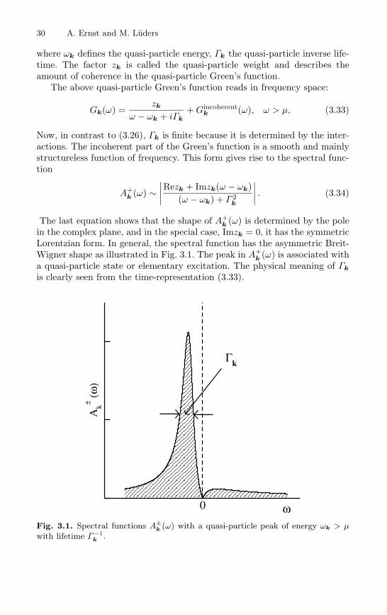
in the complex plane, and in the special case, Imzk = 0, it has the symmetricLorentzian form. In general, the spectral function has the asymmetric Breit-Wigner shape as illustrated in Fig. 3.1. The peak in A+
k (ω) is associated witha quasi-particle state or elementary excitation. The physical meaning of Γk
is clearly seen from the time-representation (3.33).
0 ω
Ak± (ω
)
Γk
Fig. 3.1. Spectral functions A±k (ω) with a quasi-particle peak of energy ωk > µ
with lifetime Γ −1k .
3 Methods for Band Structure Calculations in Solids 31
3.1.3 Self-Energy
The exact explicit expression for the single-particle Green’s function or itsspectral function is only known for a few systems. In general one has toresort to some approximations for the Green’s function. One class of approx-imations is derived via the equation of motion (3.19). It is useful to split theHamiltonian into its non-interacting part H0, which now also includes theCoulomb potential from the electron charge density, and the interaction V .Application of these equations to the definition of the Green’s function leadsto the equation of motion for the single-particle Green’s function
[i∂
∂t− H0
]Gσ,σ′(r t, r′t′)
+i∫
d3r′′v(r, r′′)〈Ψ0|T[Ψ+
σ′′(r′′t)Ψσ′′(r′′t)Ψσ(rt)Ψ+σ′(r′t′)
]|Ψ0〉
= δ(r − r′)δσ,σ′δ(t− t′). (3.35)
where
v(r, r′) =1
|r − r′| (3.36)
is the Coulomb kernel. This equation involves a two-particle Green’s function.The equation of motion of the two-particle Green’s function contains thethree-particle Green’s function, and so on. Subsequent application of 3.20generates a hierarchy of equations, which relate an n-body Green’s functionto an n+1 body Green’s function. Approximations can be obtained whenthis hierarchy is truncated at some stage by making an decoupling ansatz forhigher order Green’s functions in terms of lower order Green’s functions.
An alternative approach is to define a generalized, non-local and energy-dependent potential, which formally includes all effects due to the interaction.The equation
[i∂
∂t− H0
]Gσ,σ′(r t, r′t′)
−∑σ′′
∫d3r′′
∫dt′′Σσ,σ′′(r t, r′′t′′)Gσ′′σ1′(r′′t′′, r′t′)
= δσ,σ′δ(r − r′)δ(t− t′) (3.37)
implicitly defines this potential Σσ,σ′′(rt, r′′t′′), which is called the self-energyoperator, or mass operator.
Introducing the Green’s function of the non-interacting part of the Hamil-tonian, H0, which obeys the equation
[i∂
∂t− H0
]G0
σ,σ′(r t, r′t′) = δ(r − r′)δσ,σ′δ(t− t′) (3.38)

32 A. Ernst and M. Luders
one easily sees that the full and the non-interacting Green’s function arerelated by the Dyson equation:
Gσ,σ′(r, r′;ω) = G0σ,σ′(r, r′;ω)
+∫
d3x
∫d3x′
∑σ1.σ2
G0σ,σ1
(r,x;ω)Σσ1,σ2(x,x′;ω)Gσ2,σ′(x′, r′;ω). (3.39)
The Dyson equation can also be derived using Feynman’s diagrammatic tech-nique. More details about that can be found in standard text books on themany-body problem [3.22,3.24,3.42].
The simplest approximation for the self-energy is the complete neglect ofit, i.e.
Σ ≡ ΣH = 0, (3.40)
corresponding to the case of V = 0. Since the classical electrostatic potentialis already included in H0 this reduces to the Hartree approximation to themany-body problem. Due to the structure of the Dyson equation an approx-imation for the self-energy of finite order corresponds to an infinite orderperturbation theory. The self-energy can be evaluated by using Wick’s the-orem, Feynman’s diagram technique or by Schwinger’s functional derivativemethod.
Here we follow Hedin and Lundquist [3.29] and present an iterativemethod for generating more and more elaborate approximations to the self-energy. The self-energy is a functional of the full Green’s function and canformally also be expressed as a series expansion in a dynamically screenedinteraction W . In turn, the screened Coulomb interaction can be expressedvia the polarisation function P which is related to the dielectric function. Onecan show that all functions appearing in the evaluation of the full Green’sfunction and the self-energy, form a set of coupled integral equations whichare known as the Hedin equations. Here we present this set of equations, ascommon in literature, in the real-space/time representation
G(1, 2) = G0(1, 2) +∫
d(3, 4)G0(1, 3)Σ(3, 4)G(4, 2), (3.41)
Σ(1, 2) = i
∫d(3, 4)W (1, 3+)G(1, 4)Γ (4, 2; 3), (3.42)
W (1, 2) = v(1, 2) +∫
d(3, 4)v(1, 3)P (3, 4)W (4, 2), (3.43)
P (1, 2) = −i∫
d(3, 4)G(2, 3)Γ (3, 4; 1)G(4, 2+), (3.44)
Γ (1, 2; 3) = δ(1 − 2)δ(2 − 3) +∫
d(4, 5, 6, 7)δΣ(1, 2)δG(4, 5)
G(4, 6)G(7, 5)Γ (6, 7; 3),
(3.45)
3 Methods for Band Structure Calculations in Solids 33
where we have used an abbreviated notation (1) = (r1, σ1, t1) (the sym-bol t+ means lim η → 0(t + η) where η is a positive real number). v(1, 2) =v(r, r′)δ(t1 − t2) is the bare Coulomb potential, and Γ (1, 2; 3) is the vertexfunction containing fluctuations of the charge density. The Hedin equationsshould be solved self-consistently: one starts with Σ = 0 in (3.45), thenone calculates, with some starting Green’s function, the polarisation func-tion (3.44), the screened Coulomb function (3.43), the self-energy (3.42),and finally, with the Dyson equation (3.41), the new Green’s functionwhich should be used with the self-energy for evaluation of the vertex func-tion (3.45). This process should be repeated until the resulting Green’s func-tion coincides with the starting one. For real materials such calculations areextremely difficult, mainly because of the complexity of the vertex func-tion (3.45). In practice one usually truncates the self-consistency cycle andapproximates one or more functions, appearing in the Hedin equations (3.41)-(3.45).
Before we turn to practical approaches for the self energy, we shall considerits characteristic features following from quite general considerations [3.39].
The formal solution of Dyson’s equation (for translational invariant sys-tems in momentum space) is:
Gk(ω) =1
ω − ω0k −Σk(ω)
. (3.46)
The singularities of the exact Green’s function Gk(ω), considered as afunction of ω, determine both the excitation energies ωk of the system andtheir damping Γk. From the Lehman representation (3.30) and the Dysonequation (3.46) it follows that the excitation energy ωk is given by
ωk = ω0k + ReΣk(ωk). (3.47)
Analogously, the damping Γk is defined by the imaginary part of the self-energy:
Γk = [1 − ∂ReΣk(ωk)∂ω
]−1ImΣk(ωk). (3.48)
Using the behaviour of the Green’s function for large |ω|, we can write anassymtotic series
[Gk(ω)]−1 = ω + ak + bk/ω + ..., (3.49)
and from (3.46) it follows that the self-energy is a regular function at infinity:
Σk(ω) = −(ω0k + ak + bk/ω + ...) (3.50)
Further, since the imaginary part of the Green’s function never vanishes ex-cept on the real axis, the Green’s function Gk(ω) has no complex zeros. From
34 A. Ernst and M. Luders
the analyticity of Gk(ω) it follows that Σk(ω) is analytic everywhere in thecomplex plane with the possible exception of the real axis. Another impor-tant property of the self-energy is its behaviour in the vicinity of the chemicalpotential. If one finds
|ImΣk(ω)| ∼ (ω − µ)2 (3.51)
then the system is called a Fermi liquid [3.40]. This relation is not valid in gen-eral because one of its consequences is the existence of a sharp Fermi surface,which is certainly not present in some systems of fermions with attractiveforces between particles.
3.1.4 Kohn-Sham Approximation for the Self-Energy
In the last section we have discussed general properties of the Green’s functionand how the Green’s function is related to quasi-particle excitations. Now weshall consider some practical approaches for the self-energy, with which wecan solve the Dyson equation (3.39) on a first-principles (or ab-initio) level.
The first method we discuss is the direct application of density functionaltheory (DFT) to the calculation of the Green’s function.
DFT is one of the most powerful and widely used ab-initio methods [3.14,3.19, 3.45]. It is based on the Hohenberg and Kohn theorem [3.30], whichimplies, that all ground state properties of an inhomogeneous electron gascan be described by a functional of the electron density, and provides a one-to-one mapping between the ground-state density and the external potential.Kohn and Sham [3.34] used the fact that this one-to-one mapping holdsboth for an interacting and a non-interacting system, to define an effective,non-interacting system, which yields the same ground-state density as theinteracting system. The total energy can be expressed in terms of this non-interacting auxiliary system as:
E0 = minρ
T [ρ] +
∫vext(r)ρ(r)d3r +
12
∫ ∫ρ(r)ρ(r′)|r − r′| d3rd3r′+
+Exc[ρ] . (3.52)
Here the first term is kinetic energy of a non-interacting system with thedensity ρ, the second one is the potential energy of the external field vext(r),the third is the Hartree energy, and the exchange-correlation energy Exc[ρ]entails all interactions, which are not included in the previous terms. Thecharge density ρ(r) of the non-interacting system, which by constructionequals the charge density of the full system, can be expressed through theorthogonal and normalized functions ϕi(r) as
ρ(r) =occ.∑
i
|ϕi(r)|2. (3.53)
3 Methods for Band Structure Calculations in Solids 35
Variation of the total energy functional (3.52) with respect to the functionϕi(r) yields a set of equations, the Kohn-Sham (KS) equations, which haveto be solved self-consistently, and which are of the form of a single-particleSchrodinger equation:
[−∇2
2+ veff(r)
]ϕi(r) = εiϕi(r). (3.54)
This scheme corresponds to a single-particle problem, in which electrons movein the effective potential
veff(r) = vext(r) + vH(r) + vxc(r). (3.55)
Here vH(r) is the Hartree potential and vxc(r) = δExc(ρ(r))δρ(r) is the exchange-
correlation potential.The energy functional (3.52) provides in principle the exact ground state
energy if the exchange-correlation energy Exc[ρ] is known exactly. This func-tional is difficult to find, since this would be equivalent to the solution ofthe many-body problem, and remains a topic of current research in density-functional theory. For applications the exchange-correlation energy Exc[ρ] isusually approximated by some known functionals obtained from some sim-pler model systems. One of the most popular approaches is the local-densityapproximation (LDA), in which the exchange-correlation energy Exc[ρ] ofan inhomogeneous system is approximated by the exchange-correlation en-ergy of a homogeneous electron gas, which can be evaluated accurately, e.g.,by Quantum Monte Carlo techniques. Thereby all many-body effects areincluded on the level of the homogeneous electron gas in the local exchange-correlation potential, which depends on the electronic density and some pa-rameters obtained from many-body calculations for a the homogeneous elec-tron gas [3.57, 3.13, 3.58, 3.48, 3.47]. In many cases the LDA works well andis already for three decades widely used for great variety of systems (seereview by R.O. Jones and O. Gunnarsson [3.31], and some text books onDFT [3.14, 3.19, 3.45]). The simplicity of the local density approximationmakes it possible to solve the Kohn-Sham equation (3.54) with different ba-sis sets and for different symmetry cases. When the on-site Coulomb inter-action dominates the behaviour of electrons (strongly correlated systems),the local-density does not work well, and another approximation of Exc[ρ] isneeded.
As was already mentioned above, standard density functional theory isdesigned for the study of ground state properties. In many cases it appearsreasonable to interpret the eigenvalues εi in the one-particle equation (3.54)as excitation energies, but there is no real justification for such an interpreta-tion [3.46, 3.51]. However, also the Green’s function and thus the self-energyare, among other dependencies, functionals of the electronic density. Shamand Kohn argue that for sufficiently homogenous systems, and for energiesin the close vicinity of the Fermi-surface, the approximation
36 A. Ernst and M. Luders
Σ(r, r′;ω) ≈ vxc[ρ](r)δ(r − r′) (3.56)
should be good. The range of energies, in which this approximation can beexpected to work, depends on the effective mass of a homogeneous electrongas with a density, corresponding to some average of the actual density ofthe system. Using this approximation in the Dyson equation, one sees thatthe full Green’s function is approximated by the Green’s function of the non-interacting Kohn-Sham system, which can be expressed in terms of the KSorbitals and KS energies:
GKS,σ,σ′(r, r′;ω) = limΓ→0
(occ∑i
ϕiσ(r)ϕ∗iσ′(r′)ω − µ+ εi + iΓ
+unocc∑
i
ϕiσ(r)ϕ∗iσ′(r′)ω − µ+ εi − iΓ
)
(3.57)
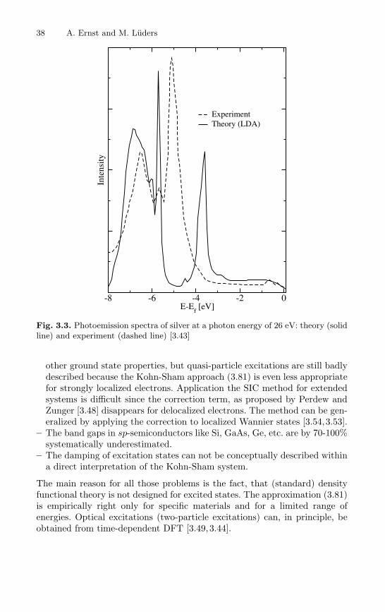
This argument explains why the otherwise unjustified interpretation of theKohn-Sham Green’s function, often gives surprisingly good results for spec-troscopy calculations. Despite the lack of a proper justification, this fact led tothe development of variety of methods on the first-principle level, which aresuccessfully applied for many spectroscopy phenomena (see recent reviewsin [3.16, 3.15]). An example, how the density functional theory within theLDA does work, is illustrated in Fig. 3.2. Here we present magneto-opticalspectra for iron calculated by a self-consistent LMTO method [3.3] and theexperimental results [3.37]. Because magneto-optics in the visible light be-longs to the low-energy spectroscopy, one can expect, that the use of theLDA is reasonable. Indeed, the calculated polar Kerr rotation and Kerr el-lipticity agree very well with the experimental curve. The theoretical curvereproduces all main features of the experimental result. With increasing en-ergy the agreement with experiment is getting worse, as expected from thedeterioration of the LDA approximation for higher energies. The theory alsocould not represent the magnitude of the experimental curve for the wholeenergy range; this is related to the damping of the quasi-particle states. Themain failure of the LDA in the description of spectroscopic phenomena isthe inability to reproduce the damping of single-particle excitation, which isgiven by the imaginary part of the self-energy (3.48) and which is not presentin the approximation (3.81). The calculated spectrum is usually artificiallysmeared by a Lorentzian broadening with some constant width Γ , but this isnot a satisfactory approximation, because in reality the damping has a morecomplicated structure. An evident case when the LDA does not work is shownin Fig. 3.3. Here we present photoemission spectra for silver at a photon en-ergy of 26 eV. The solid line shows a theoretical spectrum calculated by theseauthors using a self-consistent Green’s function method [3.18,3.38] within theLDA. The dashed line reproduces the experiment [3.43]. The low energy partof the spectra (up to 5.5 eV below the Fermi level) is adequately representedby theory. At the energy 5.1 eV below the Fermi level the experiment showsa peak corresponding to a 4d-state, which is predicted by theory at 3.6 eV

3 Methods for Band Structure Calculations in Solids 37
Fe
Ker
rel
lip
tici
ty(d
eg.)
Ker
rro
tati
on
(deg
.)LDAExper .
- 0 .5
0 .0
0 1 2 3 4 5
Ener g y ( eV)
- 0.4
- 0 .2
0 .0
Fig. 3.2. Calculated [3.3] and experimental [3.37] magneto-optical spectra of Fe
below the Fermi level. The discrepancies are related to the inadequacy of thelocal approximation of vxc(r) and to the failure of correlating Kohn-Shameigenvalues with excitation energies in the photoemission experiment. Belowwe point some serious faults of the DFT and the LDA in the description ofground state and quasi-particle state properties:
– The approximation of the exchange-correlation energy is a crucial point ofDFT calculations. Existing approximations are usually not applicable forsystems with partially filled inner shells. In presence of strong-correlatedelectrons the LDA does not provide reasonable results.
– The LDA is not completely self-interaction free. The unphysical interactionof an electron with itself can approximately be subtracted if the electron issufficiently localized [3.48]. This remarkably improves the total energy and
38 A. Ernst and M. Luders
-8 -6 -4 -2 0E-E
f [eV]
Inte
nsity
ExperimentTheory (LDA)
Fig. 3.3. Photoemission spectra of silver at a photon energy of 26 eV: theory (solidline) and experiment (dashed line) [3.43]
other ground state properties, but quasi-particle excitations are still badlydescribed because the Kohn-Sham approach (3.81) is even less appropriatefor strongly localized electrons. Application the SIC method for extendedsystems is difficult since the correction term, as proposed by Perdew andZunger [3.48] disappears for delocalized electrons. The method can be gen-eralized by applying the correction to localized Wannier states [3.54,3.53].
– The band gaps in sp-semiconductors like Si, GaAs, Ge, etc. are by 70-100%systematically underestimated.
– The damping of excitation states can not be conceptually described withina direct interpretation of the Kohn-Sham system.
The main reason for all those problems is the fact, that (standard) densityfunctional theory is not designed for excited states. The approximation (3.81)is empirically right only for specific materials and for a limited range ofenergies. Optical excitations (two-particle excitations) can, in principle, beobtained from time-dependent DFT [3.49,3.44].
3 Methods for Band Structure Calculations in Solids 39
3.2 Methods of Solving the Kohn-Sham Equation
In this chapter we describe two methods of calculating the electronic bandstructures of crystals, which is equivalent to calculating the KS Green’s func-tion. These methods represent two general approaches of solving the Kohn-Sham equation.
In the first approach the Kohn-Sham equation can be solved in somebasis set. The wave function ϕi(r) in the Kohn-Sham equation (3.54) can berepresented as linear combination of N appropriate basis functions φi(r):
ϕ(r) =N∑i
Ciφi(r) (3.58)
The basis set φi(r) should correspond to the specifics of the solving prob-lem such as the crystal symmetry, the accuracy or special features of theelectronic structures. According to the variational principle the differentialequation (3.54) represented in the basis (3.58) can be transformed to a set oflinear equations:
N∑j
(Hij − εSij)Cj = 0, j = 1, 2, .., N . (3.59)
The matrices
Hij =∫
d3rφ∗i (r)H(r)φi(r), (3.60)
Sij =∫
d3rφ∗i (r)φi(r) (3.61)
are the Hamiltionan and overlap matrices respectively. Using identity
S =(S1/2
)T
S1/2 (3.62)
the system of (3.59) can be easily transformed to the ordinary eigenvalueproblem
N∑j
(Hij − εδij)Cj = 0 (3.63)
with H =(S1/2
)THS1/2 and C = S1/2C. This ordinary eigenvalue prob-
lem (3.63) can by solved by the diagonalization of the matrix H.All variational methods differ from each other only by the choice of
the basis functions φi(r) and by the construction of the crystal poten-tial. Several efficient basis methods have been developed in last four decades

40 A. Ernst and M. Luders
and are widely used for band structure calculations of solids. A designatedchoice of basis functions serves for specific purposes. For example the lin-earized muffin-tin orbital (LMTO) method [3.1] or augmented spherical wave(ASW) [3.60] method provide very fast band structure calculations, withan accuracy which is sufficient for many applications in solids. A tight-binding representation of the basis [3.21,3.2] is very useful for different modelswith parameters determined from band structure calculations. Usually sim-ple basis methods are very fast but not very accurate. Methods with morecomplicated basis and potential constructions are appropriate for high pre-cision electronic structure calculations (see augmented plane wave (APW)method [3.52], full-potential linearized augmented plane wave (FPLAPW)method [3.10], projected augmented wave (PAW) method [3.12], full-potentiallocal-orbital minimum-basis method [3.32], several norm-conserving pseudo-potential methods [3.26,3.56]). Such methods are slower than the fast simplebasis methods mentioned above, but on modern computers they are success-fully applied even to extended systems like large super-cells, surfaces andinterfaces.
Another efficient way to solve the the Kohn-Sham equation (3.54) is theGreen’s function method. This approach is based on a corresponding math-ematical scheme of solving differential equations. Basically the method usesGreen’s function technique to transform the Schrodinger equation into anequivalent integral equation. In the crystal one can expand the crystal statesin a complete set of functions which are solutions of the Schrodinger equationwithin the unit cell, and then determine the coefficients of the expansion byrequiring that the crystal states satisfy appropriate boundary conditions. Thismethod was proposed originally by Korringa [3.35], Kohn and Rostoker [3.33],in different though equivalent form. More details about the Korringa-Kohn-Rostoker (KKR) method can be found in [3.23,3.59].
As an example of ab-initio band structure methods we shall discuss belowa high precision full-potential combined basis method [3.20, 3.17], which is aflexible generalisation of the LCAO computational scheme. Before we startthe discussion about this approach, we consider some general features whichare typical for any basis method.
In a crystal the effective potential veff(r) in the Kohn-Sham equation(3.54) is a periodic function of direct lattice vectors Ri: veff(r+Ri) = veff(r).A wave function ϕn(k; r) satisfies the Bloch theorem:
ϕn(k; r + Ri) = exp (ik · Ri)ϕn(k; r) (3.64)
Here k is a wave vector of an electron. According to the Bloch theoremsolutions of the Kohn-Sham equation (3.54) depend on the wave vector kand can generally be represented as
ϕn(k; r) = exp (ik · r)un(k; r), (3.65)
where un(k; r) is a lattice periodic function. The index n is known as theband index and occurs because for a given k there will be many independent
3 Methods for Band Structure Calculations in Solids 41
eigenstates. In any basis method the crystal states are expanded in a com-plete set of Bloch type functions. The trial wave function expanded in thebasis set should be close to the true wave function in the crystal. In crys-tals with almost free valence electrons an appropriate basis would be planewaves while the atomic-like functions are a proper choice for systems withlocalized valence electrons. Different methods of band calculations can beclassified depending on which of the two above approaches is followed. Pseu-dopotential methods or orthogonalized plane wave (OPW) method use planewaves or modified plane waves as the basis set. The tight-binding methodslike the LMTO or LCAO are based on the second concept. There are also ap-proaches which combine both delocalized and localized functions. The aim ofthese schemes is to find the best fit for true wave functions in systems whichcontain different types of electron states. Moreover, the true wave functionchanges its behaviour throughout the crystal: close to the nuclear the wavefunction is usually strongly localized and in the interstitial region it has morefree electron character. To this class of methods belongs the very popularFPLAPW method [3.10] in which the wave functions are represented by lo-calized functions in the muffin-tin sphere which are smoothly matched toplane waves in the interstitial region. Here we shall discuss another combinedbasis approach which is based on the LCAO scheme. In the LCAO method,originally suggested by Bloch [3.11], the atomic orbitals of the atoms (orions) inside the unit cell are used as basic expansion set for the Bloch func-tions. This procedure is convenient only for low energy states because theatomic orbitals are very localized and poorly describe the wave functions inthe region where the crystal potential is flat. The atomic orbitals can beoptimized as suggested in [3.21]. In this approach the atomic-like functionsare squeezed by an additional attractive potential. The extention of the basisfunctions is tuned by a parameter that can be found self-consistently [3.32].One of the main difficulties of the LCAO scheme is an abundance of multi-center integrals, which must be performed to arrive at a reasonable accuracyof band structure calculations. This difficulty is evidently most critical forsolids which have a close packed structure and therefore a great number ofneighbours within a given distance. To avoid these difficulties, one usuallyimposes some restrictions on the basis set and, as a rule, this leads to itsincompleteness, which, on the other hand, is most pressing for open struc-tures. Completeness can be regained by adding plane waves to the LCAO’s.By increasing the number of plane waves in the basis we can decrease thespatial extent of localised valence orbitals and thereby reduce the number ofmulti-center integrals. This provides a flexibility which goes far beyond usualpseudo potentials. Retaining some overlap between the local valence orbitals,we improve our plane-wave basis set and can receive a good converged Blochfunction for both valence electrons and excited states using a relatively smallnumber of plane waves. Orthogonalization of both LCAO’s and plane wavesto core states can be done before forming of Hamiltonian and overlap ma-

42 A. Ernst and M. Luders
trices. Thus, the application of combined basis sets in the combination ofLCAO’s and OPW’s allows efficiently to use advantages both approaches.
We have to solve the Kohn-Sham equation for the electronic states in aperiodic systems
[−12∇2 + veff(r)]ϕn(k; r) = εn(k)ϕn(k; r) . (3.66)
Here veff is the effective potential (3.55). The wave function ϕn(k; r) describesthe Kohn-Sham one-electron state with the wave vector k and the band indexn. Without any restriction of generality the effective potential can be splitinto two parts: a lattice sum of single local potentials decreasing smoothly tozero at the muffin tin radii and a smooth Fourier transformed potential whichis the difference between the total effective and the local potential. Thus, theeffective potential can be represented as follows
veff(r) =∑RS
vlocS (r − R − S) +
∑G
eiG·r vft(G) , (3.67)
where R and G are direct and reciprocal lattice vectors, and S is a siteposition in an unit cell. The local potential is decomposed into angular con-tributions and with our conditions has the form
vlocS (r) =
∑L
vlocSL(r)YL(r) : r ≤ rMT
0 : r > rMT ,(3.68)
where r is a normal vector along the vector r. Here YL(r) are sphericalharmonic functions with the combined index L = l,m. This decompositiongreatly simplifies the evaluation of the required matrix elements. One-electronwave functions are sought in the combined basis approach
ϕn(k; r) =∑
µ
Anµ(k)φν(k; r) +∑G
BnG(k)φG(k; r) . (3.69)
ϕµ(k; r) is the Bloch sum of localised site orbitals φµ(r − R − Sµ). Theµ−sum runs over both core and valence orbitals:µ = c, ν. The core orbitalcontributions in a valence state are needed to provide orthogonalization ofthe valence state to true core states. ϕG(k; r) ∼ ei(k+G)·r is a normalisedplane wave. We use core orbital contributions and plane wave contributionsseperately, and do not form orthogonalised plane waves (OPWs) at the outset.
In the basis set three types of functions are used: true core orbitals,squeezed local valence orbitals and plane waves. By our definition, true coreorbitals are solutions of the Kohn-Sham equation (3.66) which have negligiblenearest neighbour overlap among each other (typically less than 10−6). Thehighest fully occupied shells of each angular momentum (e.g. 2s and 2p inaluminium, or 3s and 3p in a 3d-metal) are treated like valence orbitals inmost of our calculations, because their nearest neighbour overlap is not small
3 Methods for Band Structure Calculations in Solids 43
enough to be neglected, if a larger number of plane waves is included. Thisis usually the reason for the over-completeness breakdown of OPW expan-sions. The local basis function (both core and valence) can be constructedfrom radial functions ξµ
Snl(r) which are solutions of the radial Schrodingerequation
[− 1
2r∂2
∂r2 r +l(l + 1)
2r2 + vµS(r)
]ξµSnl(r) = εµ
SnlξµSnl(r) . (3.70)
Here, in the case of core electrons (µ = c) the potential vcS(r) is the crystal
potential averaged around the center S. To obtain squeezed valence electrons(µ = ν) we use a specially prepared spherical potential by adding an artificialattractive potential to vc
S(r):
vνS(r) = vc
S(r) +(r
rν
)4
(3.71)
with a parameter rν which serves to tune the radial expansion of the basisfunctions and can be found self-consistently on the total energy minimumcondition. A useful local valence basis orbital should on the contrary rapidlydie off outside the atomic volume of its centre, but smooth enough for theBloch sums of those orbitals to provide a smooth and close approximant tothe true valence Bloch wave function so that the remaining difference betweenthe two may be represented by a few OPWs. A local basis function is denotedin the following manner
ηµ(r) = ξµSnl(r)YL(r) , (3.72)
where the lower index µ = c, ν acts as multi-index Snlm for core andvalence basis functions respectively.
The third kind of basis functions are plane waves normalised to the crystalvolume V :
ηk(r) =1√Veik·r , V = NVu , (3.73)
where N is the number of unit cells and Vu is the unit cell volume. Tosummarise, the entries in the expansion (3.66) are the basis Bloch functions
φc(k; r) ≡ (r|kc) =∑R
ηc(r − R − Sc)1√Neik·(R+Sc) , (3.74)
φν(k; r) ≡ (r|kν) =∑R
ην(r − R − Sν)1√Neik·(R+Sν) , (3.75)
φG(k; r) ≡ (r|kG) = ηk+G(r) (3.76)
The flexibility of the basis (3.72) and (3.73) consists in a balance betweenthe radial extension of the valence basis orbitals and the number of plane

44 A. Ernst and M. Luders
waves needed to converge the expansion (3.69). By reducing the parametersrν and/or the number of local basis orbitals, the number of multi-centerintegrals needed in the calculation is reduced at the price of slowing downthe convergence speed with the number of plane waves included, and viceversa. Our approach provides a full interpolation between the LCAO andOPW approaches adopting pseudo-potential features.
After the expansion of the wave functions in (3.66) we have the followingsystem of linear equations∑
µ
[(kµ′|H|kµ) − E (kµ′|kµ)]Aµ(k) = 0 , (3.77)
which gives us the sought band energies E = En(k) , n = 1, ...,M , where Mgives the rank of the coefficient matrix and corresponds to the number ofbasis functions. For the expansion coefficients Aµ
n(k) there are M differentsolutions. The equation system poses the eigenvalue problem
(H − ES)A = 0 (3.78)
with Hamilton matrix H and overlap matrix S. To solve this eigenvaluesproblem the matrix elements of the Hamiltionan and overlap matrices mustbe calculated. This is a non-trivial problem because the basis consists of threetypes of functions. Moreover the local valence functions are extended in realspace and overlap with each other and with the core orbitals. Because ofthis one needs to calculate multi-center integrals which are assumed to beindependent of the wave vector. Due to the limited space we shall not discussthis problem in the paper and refer the reader to the literature [3.20, 3.17,3.32] for more details. The secular equation (3.78) can be solved in the samemanner as discussed in the previous paper by H. Eschrig. The orthogonalityof the core orbitals allows us to restructure the matrix in (3.78) so that theeigenvalue problem will be reduced. According to this scheme the solution ofthe system of (3.78) can be carried out in the following manner. As the firststep the matrices Scλ, Sλλ, Hλλ (λ = ν,G is common index for valencebasis functions) and the energies of core states εc are determined. Then thematrix
Sλλ − S†cλScλ
is decomposed into the product of left tridiagonal matrix Slλλ and right tridi-
agonal matrix Sl†λλ with the Cholesky method. The next step is the calculation
of the inverse matrix (Slλλ)−1. Using this matrix we can calculate the matrix
Hλλ =(Sl
λλ
)−1† [Hλλ − S†cλHccScλ
] (Sl
λλ
)−1. (3.79)
After diagonalisation of the matrix Hλλ we get the matrix Uλλ, which diag-onalizes H and with this matrix the expansion coefficients A can be writtenas:

3 Methods for Band Structure Calculations in Solids 45
AT =(
1 −Scλ (Srλλ)−1
Uλλ
0 (Srλλ)−1
Uλλ
). (3.80)
The first column of the matrix A corresponds to the expansion coefficients ofcore states. According to our assumption that the core states are completelyoccupied, they do not overlap and are independent of the crystal momentumk. Therefore one of the coefficients Ac(k) is equal to one, and all other Aµ(k)are zero. The upper block of this column is hence a unit matrix 1 with the di-mension Mc×Mc, where Mc is number of the core states, and the lower blockis a zero matrix. The second column represents the expansion coefficients ofvalence functions, where the upper block includes the orthogonalization cor-rection of the valence states to the core states, and the dimension is equal toMc×Mλ. Here Mλ is the number of the valence states. The preceding schemecorresponds to the orthogonalisation corrections of the valence basis due tothe core states (e.g. see [3.21]). With this representation the Bloch wave func-tion (3.69) has a convenient form, and the estimations of the matrix elementsand the charge density are substantially simplified.
After the eigenvalue problem (3.78) is solved, we can estimate the Blochfunction (3.69) and the electronic charge density, which in our method istreated in the same manner as the crystal potential (3.67). This approachprovides a very accurate numerical representation of the charge density andthe crystal potential, which can be calculated self-consistently within thelocal density approximation.
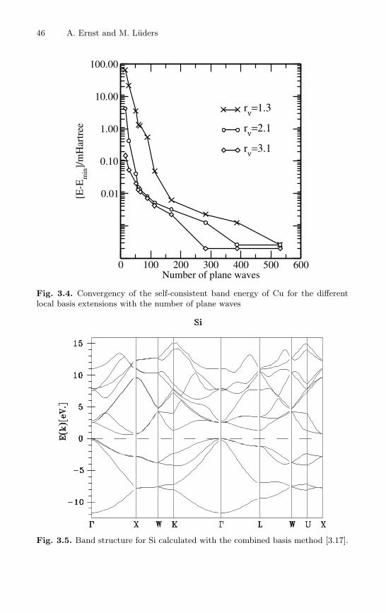
As it was already mentioned above the main advantage of the combinedbasis method is the flexibility of the basis which allows to optimize efficientlyband structure calculations without losing the high numerical accuracy. Thisfact is illustrated in Fig. 3.4 where the self-consistent band energy for Cu ispresented. In this picture we demonstrate the convergence of the band energywith the number of plane waves in the basis. The band energies have beencalculated for different parameters rν in (3.71) which regulates the extensionof the local basis functions. The overlap between the local orbitals on differentcenters is getting larger with increasing the parameter rν . Then one needsto calculate more multi-center integrals in matrix elements of the eigenvaluematrix. For smaller rν the overlap is reduced but one needs more plane wavesto obtained an accurate band structure. Another advantage of the methodis the completeness of the basis for large energy range. In many approaches,specially in linearized methods, the basis functions are appropriate only forvalence bands. This is sufficient for a study of ground state properties, butmakes the methods not applicable for the spectroscopy. In the combined basismethod the plane waves fit adequately the high lying bands which enablesaccurate calculations of spectroscopic characteristics within the local densityapproximation. Figure 3.5 shows an example of the band structure of Sicalculated by the combined basis method. The band energies are shown
along symmetry lines in the Brillouin zone. The indirected gap is 0.64 eV
46 A. Ernst and M. Luders
0 100 200 300 400 500 600Number of plane waves
0.01
0.10
1.00
10.00
100.00[E
-Em
in]/
mH
artr
ee
rν=1.3
rν=2.1
rν=3.1
Fig. 3.4. Convergency of the self-consistent band energy of Cu for the differentlocal basis extensions with the number of plane waves
Fig. 3.5. Band structure for Si calculated with the combined basis method [3.17].
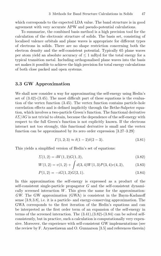
3 Methods for Band Structure Calculations in Solids 47
which corresponds to the expected LDA value. The band structure is in goodagreement with very accurate APW and pseudo-potential calculations.
To summarize, the combined basis method is a high precision tool for thecalculation of the electronic structure of solids. The basis set, consisting oflocalised valence orbitals and plane waves is appropriate for different typesof electrons in solids. There are no shape restriction concerning both theelectron density and the self-consistent potential. Typically 65 plane wavesper atom yield an absolute accuracy of ≤ 1 mRyd for the total energy for atypical transition metal. Including orthogonalised plane waves into the basisset makes it possible to achieve the high precision for total energy calculationsof both close packed and open systems.
3.3 GW Approximation
We shall now consider a way for approximating the self-energy using Hedin’sset of (3.42)-(3.45). The most difficult part of these equations is the evalua-tion of the vertex function (3.45). The vertex function contains particle-holecorrelation effects and is defined implicitly through the Bethe-Salpeter equa-tion, which involves a two-particle Green’s function. The functional derivativeδΣ/δG is not trivial to obtain, because the dependence of the self-energy withrespect to the full Green’s function is not explicitly known. If the electronsinteract not too strongly, this functional derivative is small and the vertexfunction can be approximated by its zero order expression [3.27–3.29]:
Γ (1, 2; 3) ≈ δ(1 − 2)δ(2 − 3). (3.81)
This yields a simplified version of Hedin’s set of equations:
Σ(1, 2) = iW (1, 2)G(1, 2), (3.82)
W (1, 2) = v(1, 2) +∫
d(3, 4)W (1, 3)P (3, 4)v(4, 2), (3.83)
P (1, 2) = −iG(1, 2)G(2, 1). (3.84)
In this approximation the self-energy is expressed as a product of theself-consistent single-particle propagator G and the self-consistent dynami-cally screened interaction W . This gives the name for the approximation:GW. The GW approximation (GWA) is consistent in the Baym-Kadanoffsense [3.9,3.8], i.e. it is a particle- and energy-conserving approximation. TheGWA corresponds to the first iteration of the Hedin’s equations and canbe interpreted as the first order term of an expansion of the self-energy interms of the screened interaction. The (3.41),(3.82)-(3.84) can be solved self-consistently, but in practice, such a calculation is computationally very expen-sive. Moreover, the experience with self-consistent GW implementations (seethe review by F. Aryasetiawan and O. Gunnarson [3.5] and references therein)

48 A. Ernst and M. Luders
shows that in many cases the self-consistency even worsens the results in com-parison with non-self-consistent calculations. The main reason for this is theneglect the vertex correction. Most existing GW calculations do not attemptself-consistency, but determine good approximations for the single-particlepropagator G and the screened interaction separately, i.e., they adopt a “bestG, best W” philosophy. The common choice for the single-particle propaga-tor is usually the LDA or Hartree-Fock Green’s function. Using this Green’sfunction the linear response function is obtained via the (3.84), and afterwardit is used for the calculation of the screened Coulomb interaction (3.83). Theself-energy is then determined without further iteration. Nevertheless, withthe first iteration of the GW approximation encouraging results have beenachieved. In Fig. 3.6 we show a typical result for the energy bands of MgOwithin the GWA (dotted line) compared to a conventional LDA calculation.It is clear from this plot that the GWA gap is in much better agreement withthe experimental value than the LDA results.
Below we describe briefly some existing implementations of the GWmethod. More details can be found in the original papers and in the re-views [3.5, 3.7, 3.44]. The GW integral equations (3.41),(3.82)-(3.84) can berepresented in some basis set in the real or reciprocal space and solved by
Γ X
-5
0
5
10
15
Ene
rgy
(eV
)
LDAGW
Fig. 3.6. Energy bands of MgO from KKR-LDA (solid) and GWA (dots) calcu-lations. The LDA band gap is found to be 5.2 eV, the GWA band gap is 7.7 eVwhich is in good agreement with the experimental gap of 7.83 eV.
3 Methods for Band Structure Calculations in Solids 49
matrix inversion. The basis set should be appropriate to the symmetry ofthe particular problem and should be able to represent as accuratly as pos-sible the quite distinctive behaviour of the functions, involved in the GWapproach.
– Plane wave methodsPseudo-potentials in conjunction with a plane wave basis set are widely
used in computational condensed matter theory due to their ease of useand their systematic convergence properties. Because of simplicity of theGW equations in the plane wave basis, the implementation of the GWA iseasy, and many pseudo-potential codes contain a GW part. Conventionallya pseudo-potential method can be applied for electronic structure study ofsystems with delocalised sp-electrons for which the plane wave basis con-verges rapidly. But due to recent development of the pseudo-potential tech-nique new ultra-soft pseudo-potential methods [3.56] can also be appliedto materials with localised d- and f -electrons. Most of existing pseudo-potential programs are well optimised and successfully used not only forbulk-systems but also for surfaces, interfaces, defects, and clusters. A dis-advantage of the plane wave basis is bad convergence for systems withlocalised electrons. For transition metals or f-electron systems one needsseveral thousand plane waves. Also the number of basis functions neededfor convergence is increasing with the volume of the system. Typically aplane wave GW calculation scales with N4, that makes calculations ofextended systems very expensive.
– The Gaussian basis methodRohlfing, Kruger, and Pollman [3.41] have developed a GW method whichcombines a pseudo-potential basis and localised Gaussian orbitals. In thisapproach the LDA Green function is obtained by a conventional pseudo-potential method. Afterwards the Green’s function and all GW equationsare represented in localised Gaussian orbitals. This essentially reduces thesize of the problem. Typically one needs 40-60 Gaussian functions. An-other advantage of the method is that many of integrals can be calculatedanalytically. Because the pseudo-potential part is restricted for sp-electroncompounds, the method can not be used for systems with localised elec-trons. A serious problem of the approach is the convergence of the Gaussianbasis: while a Gaussian basis can systematically converge, the number ofthe basis functions needed for convergence can be quite various for differentmaterials.
– The linearised augmented plane wave (LAPW) methodThe LAPW method is one of the most popular methods for the electronicstructure study. The basis consists of local functions, obtained from theSchrodinger equation for atomic-like potential in a muffin-tin sphere onsome radial mesh, and plane waves, which describe the interstitial region.The local functions are matched on the sphere to plane waves. Such com-bination of two different kinds of basis functions makes the LAPW method
50 A. Ernst and M. Luders
extremely accurate for systems with localised or delocalised electrons. Alsothe plane waves are better suited for high energy states, which are usuallybadly represented by a conventional tight-binding method. All this makesthe LAPW method attractive for the GW implementation. Hamada andcoworkers developed a GW method with the LAPW [3.25] and applied itto Si. 45 basis functions per Si atom were needed which corresponds to areduction by factor of five compared to plane wave calculations. But thecomputational afford is comparable with the pseudo-potential calculationsbecause the evaluation of matrix elements is more expensive. Although aGW-LAPW realisation was successfully used also for Ni [3.4], the methoddid not become very popular because of the computational costs. With fur-ther development of computer technology this method may become verypromising, as it was shown recently by Usuda and coworkers [3.55] in theGW-LAPW study in wurtzite ZnO.
– The linearised muffin-tin orbitals (LMTO) methodThe LMTO is an all-electron method [3.1,3.2] in which the wave functionsare expanded as follows,
ψnk =∑RL
χRL(r; k)bnk(RL), (3.85)
where χ is the LMTO basis, given in the atomic sphere approximation by
χRL(r,k) = ϕRL(r) +∑R′L′
ϕR′L′(r)HRL;RL′(k). (3.86)
Here ϕRL(r) = φRL(r)YL(r) is a solution to the Schrodinger equation in-side a sphere centred on an atom at site R for a certain energy εν , ϕR′L′(r)is the energy derivative of ϕRL(r) at the energy εν , and HRL;RL′(k) arethe so-called LMTO structure constants. An advantage of the LMTO isthat the basis functions do not depend on k. The LMTO method is char-acterised by high computational speed, requirement of a minimal basisset (typically 9-16 orbitals per an atom), and good accuracy in the lowenergy range.Aryasetiawan and Gunnarsson suggested to use a combination of theLMTO basis functions for solving the GW equations [3.6]. They showedthat a set of products φφ, φφ, and φφ forms a complete basis for the polar-isation function (3.84) and the self-energy (3.82). This scheme allows accu-rate description of systems with any kinds of electrons typically with 60-100product functions. A disadvantage of the approach is a bad representationof high energy states in the LMTO method, which are important for cal-culations of the polarisation function and the self-energy. Recently, Kotaniand van Schilfgaarde developed a full-potential version of the LMTO prod-uct basis method [3.36], with an accuracy which is substantially better thanthat of the conventional GW-LMTO implementation.
– The spacetime methodMost of the existing implementations of the GWA are in the real fre-

3 Methods for Band Structure Calculations in Solids 51
quency / reciprocal space representation. In this approach the evaluationof the linear response function
Pq(ω) = − i
(2π)4
∞∫−∞
dε∫
ΩBZ
d3kGLDAk (ε)GLDA
k−q (ε− ω) (3.87)
and the self-energy
Σq(ω) =i
(2π)4
∞∫−∞
dε∫
ΩBZ
d3kWk(ε)GLDAk−q (ε− ω) (3.88)
involves very expensive convolutions. In the real-space/time representationboth functions are simple products (3.84) and (3.82), which eliminates twoconvolutions in reciprocal and frequency space. The idea to chose differentrepresentations to minimise the computations is realized in the spacetimemethod [3.50]. In this scheme the LDA wave functions Φnk(r) are calcu-lated with a pseudo-potential method. Then the non-interacting Green’sfunction is analytically continuated from real to imaginary frequencies andFourier transformed into the imaginary time:
GLDA(r, r′; iτ) =
iocc.∑nk
Φnk(r)Φ∗nk(r′)eεnkτ , τ > 0
−iunocc.∑
nk
Φnk(r)Φ∗nk(r′)eεnkτ , τ < 0. (3.89)
Here r denotes a point in the irreducible part of the real space unit cellwhile r′ denotes a point in the “interaction cell” outside of which GLDA isset to zero. The linear response function is calculated in the real-space andfor imaginary time with the formula (3.84) and afterwards Fourier trans-formed from iτ to iω and from real space to reciprocal one. The screenedCoulomb interaction is evaluated as in a conventional plane wave method,and is then transformed into the real-space/imaginary time representa-tion to obtain the self-energy according the (3.82). Further, the self-energycan be Fourier transformed into the imaginary frequency axis and recipro-cal space, and analytically continuated to real frequencies. The spacetimemethod decreases substantially the computational time and makes the cal-culation of large systems accessible. A main computational problem of thespacetime method is the storage of evaluated functions (G, P , W , and Σ)in both representations.
Acknowledgements
We thank V. Dugaev and Z. Szotek for many useful discussions. A. Ernstgratefully acknowledges support from the the DFG through the Forscher-gruppe 404 “Oxidic Interfaces” and the National Science Foundation underGrant No. PHY99-07949.

52 A. Ernst and M. Luders
References
[3.1] O.K. Andersen. Linear methods in band theory. Phys. Rev. B, 12:3060, 1975.[3.2] O.K. Andersen and O. Jepsen. Explicit, first-principles tight-binding theory.
Phys. Rev. Lett., 53:2571, 1984.[3.3] V.N. Antonov, A.Y. Perlov, A.P. Shpak, and A.N. Yaresko. Calculation of the
magneto-optical properties of ferromagnetic metals using the spin-polarisedrelativistic lmto method. JMMM, 146:205, 1995.
[3.4] F. Aryasetiawan. Self-energy of ferromagnetic nickel in the gw approxima-tion. Phys. Rev. B, 46:13051, 1992.
[3.5] F. Aryasetiawan and O. Gunnarson. The GW method. Rep. Prog. Phys.,61:237, 1998.
[3.6] F. Aryasetiawan and O. Gunnarsson. Product-basis method for calculatingdielectric matrices. Phys. Rev. B, 49:16214, 1994.
[3.7] W.G. Aulbur, L. Jonsson, and J.W. Wilkins. Quasiparticle calculations insolids. In H. Ehrenreich and F. Spaepen, editors, Solid State Physics, vol-ume 54. Academic, San Diego, 2000.
[3.8] G. Baym. Self-consistent approximations in many-body systems. Phys. Rev.,127:1391, 1962.
[3.9] G. Baym and L. Kadanoff. Conservation laws and correlation functions.Phys. Rev., 124:287, 1961.
[3.10] P. Blaha, K. Schwarz, P. Sorantin, and S. Trickey. Full-Potential, LinearizedAugmented Plane Wave Programs for Crystalline Systems. Comp. Phys.Commun., 59:399, 1990.
[3.11] F. Bloch. Uber die Quantenmechanik der Elektronen in Kristallgittern. Z.Phys., 52:555–600, 1928.
[3.12] P.E. Blochel. Projector augmented-wave method. Phys. Rev. B, 50:17953,1994.
[3.13] D.J. Ceperley and L. Alder. Ground state of the electron gas by a stochasticmethod. Phys. Rev. Lett., 45:566, 1980.
[3.14] R.M. Dreizler and E.K.U. Gross. Density Functional Theory. Springer,Berlin, 1990.
[3.15] H. Dreysse, editor. Electronic Structure and Physical Properties of Solids.The Uses of the LMTO Method. Springer, Berlin, 2000.
[3.16] H. Ebert and G. Schutz, editors. Magnetic Dichroism and Spin Polarizationin Angle-Resolved Photoemission. Number 466 in Lecture Notes in Physics.Springer, Berlin, 1996.
[3.17] A. Ernst. full-potential-Verfahren mit einer kombinierten Basis fur die elek-tronische Struktur. PhD thesis, Tu Dresden, 1997.
[3.18] A. Ernst, W.M. Temmerman, Z. Szotek, M. Woods, and P.J. Durham. Real-space angle-resolved photoemission. Phil. Mag. B, 78:503, 1998.
[3.19] Eschrig. The Fundamentals of Density Functional Theory. Teubner,Stuttgart, 1996.
[3.20] H. Eschrig. Mixed basis method. In E.K.U. Gross and R.M. Dreizler, editors,Density Funtional Theory, page 549. Plenum Press, New York, 19.
[3.21] H. Eschrig. Optimized LCAO Method and the Electronic Structure of ex-tended systems. Springer-Verlag Berlin, 1989.
[3.22] A. Fetter and J. Walecka. Quantum Theory of Many-Particle Systems.McGraw-Hill, New York, 1971.

3 Methods for Band Structure Calculations in Solids 53
[3.23] A. Gonis. Green Functions for Ordered and Disordered Systems, volume 4 ofStudies in Mathematical Physics. North-Holland, Amsterdam, 1992.
[3.24] E. Gross and E. Runge. Vielteilchentheorie. Teubner, Stuttgart, 1986.[3.25] N. Hamada, M. Hwang, and A.J. Freeman. Self-energy correction for the
energy bands of silicon by the full-potential linearized augmented-plane-wavemethod: Effect of the valence-band polarization. Phys. Rev. B, 41:3620, 1990.
[3.26] D.R. Hamann, M. Scluter, and C. Chiang. Norm-conserving pseudopoten-tials. Phys. Rev. Lett, 43:1494, 1979.
[3.27] L. Hedin. Ark. Fys., 30:231, 1965.[3.28] L. Hedin. New method for calculating the one-particle green’s function with
application to the electron-gas problem. Phys. Rev., 139:A796, 1965.[3.29] L. Hedin and S. Lundqvist. Effects of electron-electron and electron-phonon
interactions on the one-electron states of solids. In F. Seitz and D. Turnbull,editors, Solid State Physics, volume 23. New York: Academic, 1969.
[3.30] P. Hohenberg and W. Kohn. Inhomogeneous electron gas. Phys. Rev.,136:B864, 1964.
[3.31] R.O. Jones and O. Gunnarson. The density functional formalism, its appli-cations and prospects. Rev. Mod. Phys., 61:689, 1989.
[3.32] K. Koepernik and H. Eschrig. Full-potential nonorthogonal local-orbitalminimum-basis band-structure scheme. Phys. Rev. B, 59:1743, 1999.
[3.33] W. Kohn and N. Rostoker. Solution of the Schrodinger equation in periodiclattices with an application to metallic lithium. Phys. Rev., 94:1111, 1954.
[3.34] W. Kohn and L.J. Sham. Self-consistent equations including exchange andcorrelation effects. Phys. Rev, 140:A1133, 1965.
[3.35] J. Korringa. Physica, 13:392, 1947.[3.36] T. Kotani and M. van Schilfgaarde. All-electron gw approximation with the
mixed basis expansion based on the full-potential lmto method. Solid StateCommunications, 121:461, 2002.
[3.37] G.S. Krinchik and V.A. Artem’ev. Magneto-optical properties of ni, co, andfe in the ultraviolet, visible and infrared parts of the spectrum. Soviet PhysicsJETP, 26:1080–1968, 1968.
[3.38] M. Luders, A. Ernst, W.M. Temmerman, Z. Szotek, and P.J. Durham. Abinitio angle-resolved photoemission in multiple-scattering formulation. J.Phys.: Condens. Matt., 13:8587, 2001.
[3.39] J.M. Luttinger. Analytic properties of single-particle propagators for many-fermion systems. Phys.Rev, 121(4):942, 1961.
[3.40] J.M. Luttinger and J.C. Ward. Ground-state energy of a many-fermionsystem. ii. Phys. Rev., 118:1417, 1960.
[3.41] P.K. M. Rohlfing and J. Pollmann. Quasiparticle band-structure calculationsfor c, si, ge, gaas, and sic using gaussian-orbital basis sets. Phys. Rev. B,48:17791, 1993.
[3.42] R. Mattuck. A Guide to Feynman Diagrams in the Many-Body Problem.McGraw-Hill, New York, 1976.
[3.43] M. Milun, P. Pervan, B. Gumhalter, and D.P. Woodruff. Photoemissionintensity oscillations from quantum-well states in the Ag/V(100) overlayersystem. Phys. Rev. B, 59:5170, 1999.
[3.44] G. Onida, L. Reining, and A. Rubio. Electronic excitations: density-functional versus many-body green’s-function approaches. Reviews of Mod-ern Physics, 72(2):601, 2002.

54 A. Ernst and M. Luders
[3.45] R.G. Parr and W. Yang. Density-Functional Theory of Atoms and Molecules.Oxford University Press, New York, 1989.
[3.46] J. Perdew. What do kohn-sham orbital energies mean? how do atoms disso-ciate? In R.M. Dreizler and da Providencia J., editors, Density FunctionalMethods in Physics, volume Physics 123 of NATO ASI Series B, page 265.Plenum, Press, New York and London, 1985.
[3.47] J.P. Perdew and Y. Wang. Accurate and simple analytic representation ofthe electron-gas correlation energy. Phys. Rev. B, 45:13 244, 1992.
[3.48] J.P. Perdew and A. Zunger. Self-interaction correction to density-functionalapproximations for many-electron systems. Phys. Rev. B, 23:5048, 1981.
[3.49] M. Petersilka, U.J. Gossmann, and E.K.U. Gross. Excitation energies fromtime-dependent density-functional theory. Phys. Rev. Lett., 76:1212, 1996.
[3.50] H.N. Rojas, R.W. Godby, and R.J. Needs. Space-time method for ab initiocalculations of self-energies and dielectric response functions of solids. Phys.Rev. Lett., 74:1827, 1995.
[3.51] L.J. Sham and W. Kohn. One-particle properties of an inhomogeneous in-teracting electron gas. Phys. Rev., 145:561, 1966.
[3.52] J.C. Slater. Damped Electron Waves in Crystals. Phys. Rev., 51:840–846,1937.
[3.53] A. Svane. Electronic structure of cerium in the self-interaction correctedlocal spin density approximatio. Phys. Rev. Lett., 72:1248, 1996.
[3.54] Z. Szotek, W.M. Temmerman, and H. Winter. Self-interaction corrected,local spin density description of the gamma –> alpha transition in ce. Phys.Rev. Lett., 72:1244, 1994.
[3.55] M. Usuda, N. Hamada, T. Kotani, and M. van Schilfgaarde. All-electron gwcalculation based on the lapw method: Application to wurtzite zno. Phys.Rev. B, 66:125101, 2002.
[3.56] D. Vanderblit. Soft self-consistent pseudopotentials in a generalized eigen-value formalism. Phys. Rev. B, 41:1990, 1990.
[3.57] U. von Barth and L. Hedin. A local exchange-correlation potential for thespin polarised case. J. Phys. C: Sol. State Phys., 5:1629, 1972.
[3.58] S.H. Vosko, L. Wilk, and M. Nusair. Accurate spin-dependent electron liquidcorrelation energies for local spin density calculations: A critical analysis.Can. J. Phys., 58:1200, 1980.
[3.59] P. Weinberger. Electron Scattering Theory of Ordered and Disordered Matter.Clarendon Press, Oxford, 1990.
[3.60] A.R. Williams, J. Kubler, and C.D. Gelatt. Cohesive properties of metalliccompounds: Augmented-spherical-wave calculations. Phys. Rev. B, 19:6094,1979.