Lab 5: Brownian motionI. Introduction

A. Tell us who you are!1. Take a picture of your lab group. This week, since we are using the external camera for the microscope images, you will have to use

Logger Pro to take the photo instead of Photo Booth.a. Open the file called Lab5.cmbl in Logger Pro.b. Insert->Video Capture.c. Select "USB Video Class Video"; this will choose the built-in camera above your computer's display.d. If it asks you to select a microphone for the sound source, pick any of the options.e. When the Video Capture window appears, click on the Options button. Under "Take Photo Type," select "Picture only." Click on OK.f. Pose for the picture, and then click on "Take Photo." The picture should appear behind the Video Capture window.g. Click on the picture, and copy and paste it here:

2. Tell us your names!

a.B. Background

1. For a nice description of Brownian motion, see the handout viscosity-brownian.pdf (double-click the image to view the document):

Why does a constant force on an object in a viscous medium produce a

constant (terminal) velocity?

You know that the viscous drag force Fdrag is proportional to the velocity v (and in the

opposite direction); we’ll use the symbol f to represent the coefficient of proportionality:

Fdrag = –fv

When an object reaches terminal velocity, the drag force is equal and opposite to the

constant external force, so the velocity is constant:

Fext = –Fdrag so

!

v =Fext

f

We seek a microscopic model for viscosity that can explain this observation. As the

object is being pulled through the fluid by a constant force, the object is also subjected to

numerous microscopic collisions with the molecules of the fluid. Let’s assume that these

collisions are periodic: there is one collision per time !t. Let’s also assume that as a

result of each collision, our object’s velocity is “reset” to some random value vo. Then,

before the next collision, the object moves freely, influenced only by the constant

external force. The constant force produces a constant acceleration a = Fext/m, so the

object’s velocity is given by the usual kinematic equation for constant acceleration:

!

v = vo

+Fext

m

"

# $

%

& ' (t

For a constant “downward” force (for instance, a gravitational force) the velocity of such

a particle might look like this:

2. Key equations from the handouta. Definition of viscous friction coefficient f:

f = Fext/v(1)

For a solid sphere of radius r, f = 6πμr (Stokes' Law)b. Relationship of f to microscopic random-walk model:

f = 2m/∆tc. Definition of diffusion constant D:

D = (∆x)2/2∆td. Mean squared displacement is linear in time:

<x2> = 2Dte. Einstein-Smoluchowski relation between D, f, and average thermal energy kT:

Df = kTC. Materials

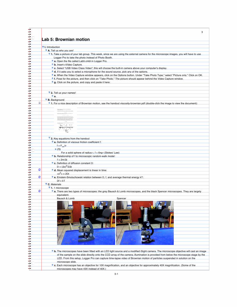
1. 1 microscopea. There are two types of microscopes: the grey Bausch & Lomb microscopes, and the black Spencer microscopes. They are largely

equivalent.Bausch & Lomb Spencer

b. The microscopes have been fitted with an LED light source and a modified iSight camera. The microscope objective will cast an image of the sample on the slide directly onto the CCD array of the camera; illumination is provided from below the microscope stage by the LED. From this setup, Logger Pro can capture time-lapse video of Brownian motion of particles suspended in solution on the microscope slide.

c. Each microscope has an objective for 10X magnification, and an objective for approximately 40X magnification. (Some of the microscopes may have 43X instead of 40X.)

d. Each microscope also has two focus knobs. The larger/upper knob is for coarse focus adjustments, and the lower one is for fine adjustments.

e. The on/off switch for the LED is located just below the 9-volt battery.

3-1

3

d. Each microscope also has two focus knobs. The larger/upper knob is for coarse focus adjustments, and the lower one is for fine adjustments.

e. The on/off switch for the LED is located just below the 9-volt battery.2. Microscope slides

a.

b. The slides are well slides, which means they have a slight depression in the center to hold the sample.3. Cover slips

II. Procedure.A. Measure the Brownian motion of a 1-micron polystyrene sphere in water.

1. Familiarize yourself with your microscope.2. Prepare a sample.

a. A sample preparation area is next to the sink. There are several types of microsphere solution in plastic bottles, each labeled with a diameter. We'll start with the 1-micron spheres.

b. Using the pipette, place a drop or two of solution into one of the well slides, and cover it with a cover slip. Try not to trap air bubbles under the cover slip.

c. Invert the slide onto a Kimwipe and tap it gently to remove excess solution.d. After a few minutes the edges will dry, and the cover slip will become lightly stuck to the well slide. This should provide a sample with

minimal evaporation. Evaporation would cause an overall drift of particles in the direction of the fastest evaporation, which is something we don't want.

3. Observe the sample under the microscope.a. Load the sample into the microscope by clipping the slide onto the microscope stage.b. Go to page 2 of the Logger Pro file and insert another video capture, this time using the IIDC Firewire camera.

(1) Sometimes the Video Capture window appears in a flaky way: covering the buttons which should appear on the right hand side of the window. Closing it, waiting a few seconds, then reopening it usually solves this problem.

c. If it asks you for a resolution, select 800x600. If it asks you for the audio source, pick any of the options.d. Focus an image onto the camera. Use the 10X objective first, and learn how to focus on spheres throughout the depth of your sample.e. Switch to the 40X objective, which you will use to collect data, and master the more delicate task of focusing on spheres at this higher

magnification. Be careful! On the 40X objective, it is very possible to break your slide and/or cover slip by trying to move the objective too close to the sample using the coarse focus knob.

f. Observe the microspheres for long enough to convince yourself that the particles are diffusing with minimal overall drift. The solution should be dense enough that a few spheres are within the field of view.

4. Collect a video capture of the Brownian motion of the spheres.a. In the Video Capture window, click on the Options button.b. Check the box marked Time-Lapse Capture. Choose a capture interval of 5 seconds between frames.c. Set the capture duration to 300 seconds (5 minutes).d. Set "Capture File Name Starts With" to something descriptive, such as "1 micron."e. Click on OK.f. Click on Start Time Lapse.g. Wait for 5 minutes. Every 5 seconds, the video will appear to freeze momentarily while Logger Pro records a frame.h. When it is finished, the captured video will appear behind the Video Capture window. Close the Video Capture window.i. Save your Logger Pro file.

5. Set the scale for your captured video.a. In Logger Pro, select Insert → Picture → Picture Only.b. On each computer desktop folder are two photos of a scale with 10 micron divisions, taken at 10X and 40X on your microscope. Select

the appropriate photo to include on your LoggerPro page.c. Re-position the picture underneath and in line with the time-lapse video, but overlapping slightly so that you can still see the scale

markings when the video window is on top.d.

Click on the icon to bring up the video analysis functions. Click the button to set the length scale.e. Use the scale markings in the adjacent photo to give you a length reference, but click and drag in the video window (not the picture

window) to set the scale. Enter the scale in microns (you can use the abbreviation "um" if you like).f. The distance between the small divisions is 10 microns, hence the distance between the large divisions is 50 microns. As a point of

reference, the entire window should be something like 70 or 80 microns across on 40X magnification. When you have finished setting the scale, the screen should look something like this:(1)

3-2

(1)

6. Quickly scroll through the entire movie (by dragging the circle through the scroll bar) to see if there is a microsphere that appears to stay in the picture for the duration of the capture. This is preferable for the video analysis; however, if there is no such sphere, that's okay too. The other, and more important, thing to check for, is that there is minimal overall drift of the entire sample in the same direction. If there is significant drift, it is probably best to wait a few minutes and try again. If that doesn't work, just make a new sample.

7. Add points to your video analysis.a. Choose a sphere that you are going to follow for the 5 minutes. Again, it is preferable but not essential to choose one that stays in view

the whole time. However, make sure to choose a sphere that appears to be moving freely, rather than one that is stuck to the glass (or is perhaps not a microsphere at all, but just a smudge on the microscope or camera lens!).

b.Return to the start of the video by clicking the button.

c.Click the button to begin adding points.

d. Click on the center of the sphere to add the data point there.e. Logger Pro automatically advances one frame after each click, so you can just keep clicking on the position of the sphere in each frame.f. If no single microsphere is visible for the entire video, just switch to a new one part way through. Since only the differences in position

between adjacent points are used in the analysis, you will only lose one data point; however, be sure to remember that you did this so you can strike out the phony data point later when you do your analysis. (It will end up looking as if the microsphere jumped all the way across the screen in a single 5-second interval.)

8. Analyze the data.a.

Open the Data Browser ( button) and use it to rename the Video Analysis data set to "1 micron" or something else descriptive.b. Make a graph of Y position vs X position.

(1) You can use your existing graph of X and Y vs time. Just click on where it says Time on the horizontal axis and change it to X.(2) Then click on where it says "X Y" on the vertical axis and change it to just Y.(3) Double-click on the graph and uncheck Point Protectors, but check the box for Connect Points.(4) You should now see essentially the path traced by your sphere as it executed its five minute random walk. Paste a copy here:

c. Move to page 3 in the Logger Pro file. You should see a data table with columns for X, Y, X velocity, and Y velocity.d. In your video analysis data set (or whatever it is now called), define a calculated column labeled "Delta x" to give the diifference in X

position between adjacent times.(1) Double-click on the column heading for X velocity. We won't need the X velocity, so we'll just change this column to suit our

purposes better. Rename it "Delta x" and change the units from microns per second to just microns. If you want to give it a short name, too, feel free to do that.

(2) In the equation for column definition, where it says derivative("X"), replace it with the "delta" function applied to the "X" column.(a) 3-3

(a)

(3) This new column will be one row shorter than the X column, and will show you the change in X during each 5-second interval.(4) Change Y velocity into a column of deltas for the Y values in the same way.(5) If you had to switch spheres during your video, eliminate the spurious data point by striking through it in the "Delta x" and "Delta y"

columns (not in the original X or Y column) using Apple-minus.e. Make a graph that shows Delta x and Delta y vs time.

(1) Insert → Graph.(2) Double-click the graph, go to Axes Options, and check the boxes for Delta x and Delta y in the correct data set.(3)

Click on the Statistics button to generate statistics for Delta x and Delta y. (Check both boxes when it asks you which column to compute statistics for.)

(4) Paste the graph here, with the statistics box showing the mean and standard deviation of both Delta x and Delta y:

(5) For delta x:

(a) mean = (b) standard deviation = (c) standard error = (d) If there is no overall drift, we expect the mean to be zero. How many standard errors away from zero is it?

If the mean is more than two SE away from zero, you may have had excessive drift and the rest of the analysis will not work very well. Talk to a TF.

(6) For delta y: (a) mean = (b) standard deviation = (c) standard error = (d) How many standard errors away from zero?

f. When you get to this point, let a TF know so that they can gather your data for the whole class to use later. Now would also be a fine time to save your work.

g. Make a histogram of the "Delta x" and "Delta y" columns.(1) Insert → Additional Graphs → Histogram.(2) Double-click on the histogram to select which columns to display, as well as adjust the settings for the bin width and start position.(3) Can you fit a Gaussian to the histograms?

(a)Click the Curve Fit button.

(b) Select Delta x and click OK.(c) Select PS2 Gaussian and try an automatic fit.(d) If it doesn't work (or the fit looks very bad), try changing the bin width of the histogram.(e) Repeat for Delta y.

(4) Recall that the mean and standard deviation of the Gaussian are given by the parameters B and C, respectively.(a) delta x B = (b) delta x C = (c) How do these compare with the mean and standard deviation you calculated directly from the data?(d) delta y B = (e) delta y C =

(5) Paste a copy of your histogram here.

3-4

(e) delta y C = (5) Paste a copy of your histogram here.

h. Because every measurement is independent ("a random walk has no memory"), we are going to treat our two five-minute random

walks as 120 separate short random walks, each lasting five seconds.(1) With this new interpretation, each value of Delta x or Delta y is really just a final displacement, x, of such a short walk.(2) The squared displacement is then just (Delta x)2. We are interested in finding the mean squared displacement, <x2>; but this is just

the square of the standard deviation of the Delta x and Delta y values. Why?(a) Recall the defintion of standard deviation: the square root of the average squared distance from the mean.

σ = √(∑(x-<x>)2/N)(b) The mean value <x> is zero, if there is no drift. So σ2 = ∑(x-0)2/N = ∑x2/N = <x2>.

(3) Calculate the mean squared displacement of your 120 five-second random walks.(a) The mean squared displacement of your 60 Delta x walks is just the standard deviation squared for that data set, and likewise for

Delta y.(b) To combine them into a single result, we take the average of the two values--but we average after squaring, not before.(c) <x2> =

(4) Now we'll try to determine the uncertainty in our calculated value of <x2>.(a) One useful piece of information is that the fractional uncertainty in the standard deviation of a set of values is:

(uncertainty in σ)/σ = 1/√(2(N-1))(b) We would like to calculate the uncertainty in σ2, which can be obtained from the error propagation formula:

(uncertainty in σ2)/σ2 = 2 (uncertainty in σ)/σ(c) Finally, when we average two values a and b, the uncertainty in the average is given by another error propagation formula:

uncertainty in ½(a+b) = ½√((uncertainty in a)2 + (uncertainty in b)2)(d) Calculate the uncertainty in your value of the mean squared displacement.

uncertainty = i. Calculate the diffusion constant D.

(1) Recall that the mean squared displacement is linear in time. What is the value of t for your data?(2) D = (3) Uncertainty in D =

j. Deduce a value for Boltzmann's constant k from the Einstein-Smoluchowski equation.(1) You may need the following information:

(a) Diameter of microsphere = 1.025 microns (1.025 x 10-6 m) +/- 0.010 microns(b) Viscosity of microsphere solution = 1.20 x 10-3 Pa s(c) Temperature: depends on the day. The TFs will tell you the temperature in the room.

(2) k = (3) Uncertainty in k = (4) What are the units of k?

k. Finally, using R = 8.31 J/K mol, calculate Avogadro's number, NA = R/k.(1)

NA = (2)

Uncertainty = 9. After the TFs have collected data from every group, they will show you some pretty graphs, from which we can also derive a value of D

measured by the whole class. Record that value here:

(If you get here before the rest of the class has submitted their data, go on ahead and come back to it later.)10. After observing a sample, clean and reuse the well slide, and replace it in the plastic case when you finish. Dispose of cover slips and

pipettes in the blue glass disposal box.B. Measure the Brownian motion of larger spheres and determine the dependence of D on radius.

1. Prepare a sample.a. A sample preparation area is next to the sink. There are several types of microsphere solution in plastic bottles, each labeled with a

diameter. This time, take a different diameter (2, 3, 6, or 10 microns). Look at the whiteboard at the back of the room to see which diameter to use.

b. Using the pipette, place a drop or two of solution into one of the well slides, and cover it with a cover slip. Try not to trap air bubbles under the cover slip.

c. Invert the slide onto a Kimwipe and tap it gently to remove excess solution.d. After a few minutes the edges will dry, and the cover slip will become lightly stuck to the well slide. This should provide a sample with

minimal evaporation. Evaporation would cause an overall drift of particles in the direction of the fastest evaporation, which is something we don't want.

2. Observe the sample under the microscope.a. Load the sample into the microscope by clipping the slide onto the microscope stage.b. Go to page 4 of the Logger Pro file and insert another video capture, this time using the IIDC Firewire camera.

(1) Sometimes the Video Capture window appears in a flaky way: covering the buttons which should appear on the right hand side of the window. Closing it, waiting a few seconds, then reopening it usually solves this problem.

c. Focus an image onto the camera.d. Observe the microspheres for long enough to convince yourself that the particles are diffusing with minimal overall drift. The solution

should be dense enough that a few spheres are within the field of view.3. Collect a video capture of the Brownian motion of the spheres.

a. In the Video Capture window, click on the Options button.b. Check the box marked Time-Lapse Capture. Choose a capture interval of 5 seconds between frames.c. Set the capture duration to 300 seconds (5 minutes).d. Set "Capture File Name Starts With" to something descriptive, such as "2 microns" or "6 microns."

3-5

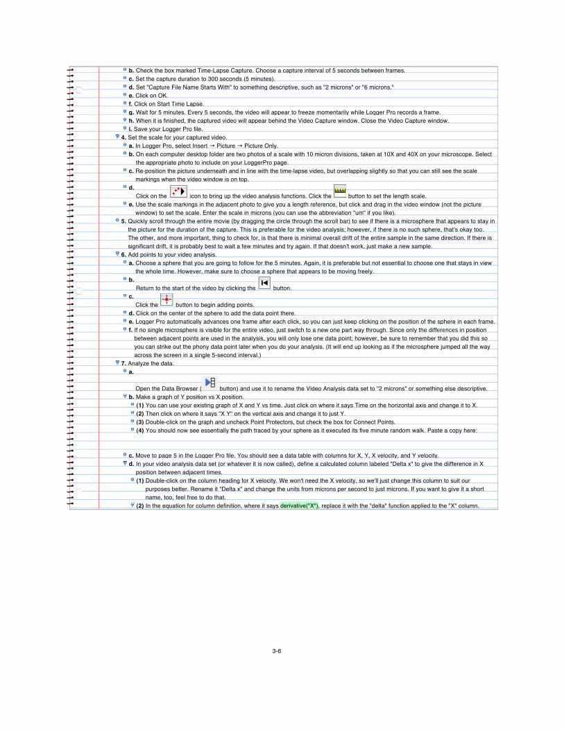
b. Check the box marked Time-Lapse Capture. Choose a capture interval of 5 seconds between frames.c. Set the capture duration to 300 seconds (5 minutes).d. Set "Capture File Name Starts With" to something descriptive, such as "2 microns" or "6 microns."e. Click on OK.f. Click on Start Time Lapse.g. Wait for 5 minutes. Every 5 seconds, the video will appear to freeze momentarily while Logger Pro records a frame.h. When it is finished, the captured video will appear behind the Video Capture window. Close the Video Capture window.i. Save your Logger Pro file.

4. Set the scale for your captured video.a. In Logger Pro, select Insert → Picture → Picture Only.b. On each computer desktop folder are two photos of a scale with 10 micron divisions, taken at 10X and 40X on your microscope. Select

the appropriate photo to include on your LoggerPro page.c. Re-position the picture underneath and in line with the time-lapse video, but overlapping slightly so that you can still see the scale

markings when the video window is on top.d.

Click on the icon to bring up the video analysis functions. Click the button to set the length scale.e. Use the scale markings in the adjacent photo to give you a length reference, but click and drag in the video window (not the picture

window) to set the scale. Enter the scale in microns (you can use the abbreviation "um" if you like).5. Quickly scroll through the entire movie (by dragging the circle through the scroll bar) to see if there is a microsphere that appears to stay in

the picture for the duration of the capture. This is preferable for the video analysis; however, if there is no such sphere, that's okay too. The other, and more important, thing to check for, is that there is minimal overall drift of the entire sample in the same direction. If there is significant drift, it is probably best to wait a few minutes and try again. If that doesn't work, just make a new sample.

6. Add points to your video analysis.a. Choose a sphere that you are going to follow for the 5 minutes. Again, it is preferable but not essential to choose one that stays in view

the whole time. However, make sure to choose a sphere that appears to be moving freely.b.

Return to the start of the video by clicking the button.c.

Click the button to begin adding points.d. Click on the center of the sphere to add the data point there.e. Logger Pro automatically advances one frame after each click, so you can just keep clicking on the position of the sphere in each frame.f. If no single microsphere is visible for the entire video, just switch to a new one part way through. Since only the differences in position

between adjacent points are used in the analysis, you will only lose one data point; however, be sure to remember that you did this so you can strike out the phony data point later when you do your analysis. (It will end up looking as if the microsphere jumped all the way across the screen in a single 5-second interval.)

7. Analyze the data.a.

Open the Data Browser ( button) and use it to rename the Video Analysis data set to "2 microns" or something else descriptive.b. Make a graph of Y position vs X position.

(1) You can use your existing graph of X and Y vs time. Just click on where it says Time on the horizontal axis and change it to X.(2) Then click on where it says "X Y" on the vertical axis and change it to just Y.(3) Double-click on the graph and uncheck Point Protectors, but check the box for Connect Points.(4) You should now see essentially the path traced by your sphere as it executed its five minute random walk. Paste a copy here:

c. Move to page 5 in the Logger Pro file. You should see a data table with columns for X, Y, X velocity, and Y velocity.d. In your video analysis data set (or whatever it is now called), define a calculated column labeled "Delta x" to give the diifference in X

position between adjacent times.(1) Double-click on the column heading for X velocity. We won't need the X velocity, so we'll just change this column to suit our

purposes better. Rename it "Delta x" and change the units from microns per second to just microns. If you want to give it a short name, too, feel free to do that.

(2) In the equation for column definition, where it says derivative("X"), replace it with the "delta" function applied to the "X" column.(a)

3-6

(a)

(3) This new column will be one row shorter than the X column, and will show you the change in X during each 5-second interval.(4) Change Y velocity into a column of deltas for the Y values in the same way.(5) If you had to switch spheres during your video, eliminate the spurious data point by striking through it in the "Delta x" and "Delta y"

columns (not in the original X or Y column) using Apple-minus.e. Make a graph that shows Delta x and Delta y vs time.

(1) Insert → Graph.(2) Double-click the graph, go to Axes Options, and check the boxes for Delta x and Delta y in the correct data set.(3)

Click on the Statistics button to generate statistics for Delta x and Delta y. (Check both boxes when it asks you which column to compute statistics for.)

(4) Paste the graph here, with the statistics box showing the mean and standard deviation of both Delta x and Delta y:

(5) For delta x:

(a) mean = (b) standard deviation = (c) standard error = (d) If there is no overall drift, we expect the mean to be zero. How many standard errors away from zero is it?

If the mean is more than two SE away from zero, you may have had excessive drift and the rest of the analysis will not work very well. Talk to a TF.

(6) For delta y: (a) mean = (b) standard deviation = (c) standard error = (d) How many standard errors away from zero?

f. Save your work.g. Make a histogram of the "Delta x" and "Delta y" columns.

(1) Insert → Additional Graphs → Histogram.(2) Double-click on the histogram to select which columns to display, as well as adjust the settings for the bin width and start position.(3) Can you fit a Gaussian to the histograms?

(a)Click the Curve Fit button.

(b) Select Delta x and click OK.(c) Select PS2 Gaussian and try an automatic fit.(d) If it doesn't work (or the fit looks very bad), try changing the bin width of the histogram.(e) Repeat for Delta y.

(4) Recall that the mean and standard deviation of the Gaussian are given by the parameters B and C, respectively.(a) delta x B = (b) delta x C = (c) How do these compare with the mean and standard deviation you calculated directly from the data?(d) delta y B = (e) delta y C =

(5) Paste a copy of your histogram here.

h. Because every measurement is independent ("a random walk has no memory"), we are going to treat our two five-minute random

3-7

(5) Paste a copy of your histogram here.

h. Because every measurement is independent ("a random walk has no memory"), we are going to treat our two five-minute random walks as 120 separate short random walks, each lasting five seconds.(1) With this new interpretation, each value of Delta x or Delta y is really just a final displacement, x, of such a short walk.(2) The squared displacement is then just (Delta x)2. We are interested in finding the mean squared displacement, <x2>; but this is just

the square of the standard deviation of the Delta x and Delta y values. Why?(a) Recall the defintion of standard deviation: the square root of the average squared distance from the mean.

σ = √(∑(x-<x>)2/N)(b) The mean value <x> is zero, if there is no drift. So σ2 = ∑(x-0)2/N = ∑x2/N = <x2>.

(3) Calculate the mean squared displacement of your 120 five-second random walks.(a) The mean squared displacement of your 60 Delta x walks is just the standard deviation squared for that data set, and likewise for

Delta y.(b) To combine them into a single result, we take the average of the two values--but we average after squaring, not before.(c) <x2> =

(4) Now we'll try to determine the uncertainty in our calculated value of <x2>.(a) One useful piece of information is that the fractional uncertainty in the standard deviation of a set of values is:

(uncertainty in σ)/σ = 1/√(2(N-1))(b) We would like to calculate the uncertainty in σ2, which can be obtained from the error propagation formula:

(uncertainty in σ2)/σ2 = 2 (uncertainty in σ)/σ(c) Finally, when we average two values a and b, the uncertainty in the average is given by another error propagation formula:

uncertainty in ½(a+b) = ½√((uncertainty in a)2 + (uncertainty in b)2)(d) Calculate the uncertainty in your value of the mean squared displacement.

uncertainty = i. Calculate the diffusion constant D.

(1) Recall that the mean squared displacement is linear in time. What is the value of t for your data?(2) D = (3) Uncertainty in D = (4) After the TFs have collected data from every group, they will show you some pretty graphs, from which we can also derive a value

of D measured by the whole class. Record that value here: (If you get here before the rest of the class has submitted their data, go on ahead and come back to it later.)

j. Write your result on the whiteboard at the back of the classroom. The TFs will collect the data and make a graph of the whole class's results.

8. After observing a sample, clean and reuse the well slide, and replace it in the plastic case when you finish. Dispose of cover slips and pipettes in the blue glass disposal box.

C. If you finish early, it might be fun to look at some other samples.III. Conclusion

A. Draw a creative picture about something you learned in the lab. Use the following trick to take a picture of it using Photo Booth: open Photo Booth while Logger Pro has a video capture window open. Since Photo Booth can't access the external camera while Logger Pro is using it, it will revert to the built-in camera. Take a snapshot of your picture (remember to check the option for Auto-Flip new photos) and paste it below.

B. Submit your work to the dropbox on the website.

1. Save all of your work.2. Open a Finder window and locate the folder where you have saved your Logger Pro files (Lab5.cmbl and the two movies you captured)

and your NoteBook file (this file).3. Click on one file, and then shift-click on the others so that all four will be selected. 4. Under the File menu, select Create Archive of 4 items. You should see a new file appear in the folder named Archive.zip.5. Rename Archive.zip to a filename that includes “Lab 5” and all three of your names.6. Now open Safari (the web browser) and go to the the course website for your class, either PS2 or P11a (by default, Safari will open to the

PS2 website) and log in with your Harvard ID number.7. Click on the Labs page and find the dropbox with your lab day and time and click on it. Make sure you use the correct dropbox; otherwise

your TFs will never be able to find your lab report.8. Click on Upload File and upload the archive file you created. For a title, call it “Lab 5 report.” Then click Submit. It's a big file this week

because of the two movies, so it could take a little while.9. Make absolutely sure the file ends up in the (correct) dropbox before you leave.10. You only need to submit one report for the three of you, but you may want to email the file to your lab partners since only the person who

submitted the file (i.e. the person who entered their Harvard ID to log into the website) can later view it from the dropbox on the website.C. That's it! We hope you enjoyed the lab. Perhaps we'll see you next semester.

3-8