3. Forecasting

Homework problems: 2,4,5,6,7,11,12,14.

3.1. Providing Appropriate Forecast Information

The forecasting process involves much more than just the estimation of future demand. The forecast also needs to take into consideration the intended use of the forecast, the methodology for aggregating and disaggregating the forecast, and assumptions about future conditions.

Selection of an appropriate forecast method is determined by different levels of aggregation, cost of data acquisition and processing, length of forecast (timeframe), top management involvement, forecast frequency, etc.

Figure 3.1

3.1. Forecast Information

• The forecast information and technique must match the intended application:

For strategic decisions such as capacity or market expansion highly aggregated estimates of general trends are necessary.

Sales and operations planning (SOP) activities require more detailed forecasts in terms of product families and time periods.

Master production scheduling (MPS) and control demand highly detailed forecasts, which only need to cover a short period of time.

3.1.1 Forecasting for Strategic Business Planning

Forecast is presented in general terms (sales dollars, tons, hours)

Aggregation level may be related to broad indicators (gross national product (GNP), income)

Causal models and regression/correlation analysis are typical tools

Managerial insight is critical and top management involvement is intense

Forecast is generally prepared annually and covers a period of years

3.1.2 Forecasting for Sales and Operations Planning

Forecast is presented in aggregate measures (dollars, units)

Aggregation level is related to product families (common family measurement)

Forecast is typically generated by summing forecasts for individual products.

Managerial involvement is moderate, and limited to adjustment of aggregate values

Forecast is generally prepared several times each year and covers a period of several months to a year.

3.1.3 Forecasting for MPS and Control

Forecast is presented in terms of individual products (units, not dollars)

Forecast is typically generated by mathematical procedures, often using softwareProjection techniques are commonAssumption is that the past is a valid predictor of

the future

Managerial involvement is minimal.

Forecast is updated almost constantly and covers a period of days or weeks.

3.2. Regression Analysis & Decomposition

Regression identifies a relationship between two or more correlated variables.Linear regression is a special case where the

relationship is defined by a straight line, used for both time series and causal forecasting.

Data should be plotted to see if they appear linear before using linear regression.

Y = a + bXY is value of dependent variable, a is the y-

intercept of the line, b is the slope, and X is the value of the independent variable.

3.2 Least Squares Method

• Objective–find the line that minimizes the sum of the squares of the vertical distance between each data point and the line

Y – calculated dependent variable value

yi – actual dependent variable point

a – y intercept

b – slope of the line

x – time period

Y = a + bx

2222

211 )()()( ii YyYyYySquaresofSum

See Fig. 3.2

Least Squares Regression Line (Fig.3.2)

Regression errors are the vertical distance from the point to the line

Least Squares Equation (3.3)

22 )(xnx

yxnxyb

22

xxn

yxxynb

Or

Least Squares Example (Fig. 3.3)

Quarter (x) Sales (y) xy x2 y2 Y

1 600 600 1 360,000 801.3

2 1,550 3,100 4 2,402,500 1,160.9

3 1,500 4,500 9 2,250,000 1,520.5

4 1,500 6,000 16 2,250,000 1,880.1

5 2,400 12,000 25 5,760,000 2,239.7

6 3,100 18,600 36 9,610,000 2,599.4

7 2,600 18,200 49 6,760,000 2,959.0

8 2,900 23,200 64 8,410,000 3,318.6

9 3,800 34,200 81 14,440,000 3,678.2

10 4,500 45,000 100 20,250,000 4,037.8

11 4,000 44,000 121 16,000,000 4,397.4

12 4,900 58,800 144 24,010,000 4,757.1

Sum 78 33,350 268,200 650 112,502,500

Least Squares Example (Fig. 3.2)

6666.441)6153.359(5.617.779,2 xbya

6153.3595.6*12650

17.779,2*5.6*12200,268

)( 222

xnx

yxnxyb

xbxaY 6.35967.441

Least Squares Example

Quarter Calculation Forecast

13 Y13=441.6+359.6(13) 5,119.4

14 Y14=441.6+359.6(14) 5,476.0

15 Y15=441.6+359.6(15) 5,835.6

16 Y16=441.6+359.6(16) 6,195.2

Standard Error of Estimate (Syx) – how well the line fits the data

10

)1.757,4900,4()5.520,1500,1()9.160,1550,1()3.801600(

2

)( 22221

2

n

YyS

n

iii

yx

xbxaY 6.35967.441

=363.9

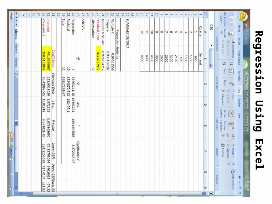
Reg

ression

Usin

g E

xcel

Time Series Decomposition

A time series can consist of one or more components of demand

Trend–the long term growth (or

decrease) of demand

Seasonal–Changes in

demand associated with portions of the year (may be

additive or multiplicative)

Cyclical–repetitive

patterns not associated with

seasonal demand

Autocorrelation–changes in

demand associated with

previous demand levels

Random–changes in

demand that can’t be linked to a specific cause

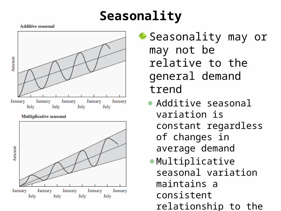
Seasonality

Seasonality may or may not be relative to the general demand trend

Additive seasonal variation is constant regardless of changes in average demand

Multiplicative seasonal variation maintains a consistent relationship to the average demand (this is the more common case)

Seasonality

Additive seasonal variation is constant regardless of changes in average demand

Forecast=Trend + Seasonal

Multiplicative seasonal variation maintains a consistent relationship to the average demand (this is the more common case)

Forecast= Trend x Seasonal factors

Seasonal Factor/Index

To account for seasonality within the forecast, the seasonal factor/index is calculated.

The amount of correction needed in a time series to adjust for the season of the year

Season Past Sales

Average Sales for Each Season

Seasonal Factor

Spring 200 1000/4=250 Actual/Average=200/250=0.8

Summer 350 1000/4=250 350/250=1.4

Fall 300 1000/4=250 300/250=1.2

Winter 150 1000/4=250 150/250=0.6

Total 1000

Seasonal Factor/Index

• If we expect (forecast) next year’s sales to be 1,100 units, the seasonal forecast is calculated using the seasonal factors:

Season ExpectedSales

Average Sales for Each Season

Seasonal Factor

Forecast

Spring 1100/4=275 X 0.8 = 220

Summer

1100/4=275 X 1.4 = 385

Fall 1100/4=275 X 1.2 = 330

Winter 1100/4=275 X 0.6 = 165

Total 1,100

Seasonality–Trend and Seasonal Factor

Quarter Amount

I – 2008 300

II – 2008 200

III – 2008 220

IV – 2008 530

I – 2009 520

II – 2009 420

III – 2009 400

IV - 2009 700

Trend = 170 +55t

Estimate of trend, use linear regression software to obtain more precise results

Seasonality–Trend and Seasonal Factor

Seasonal factors are calculated for each season, then averaged for similar seasons

Seasonal Factor = Actual/Trend

Seasonality–Trend and Seasonal Factor

Forecasts for 2010 are calculated by extending the linear regression and then adjusting by the appropriate seasonal factor

FITS–Forecast Including Trend and Seasonal Factors

Decomposition Using Least Squares Regression

1. Decompose the time series into its components

a. Find seasonal component

b. Deseasonalize the demand

c. Find trend component

2. Forecast future values for each componenta. Project trend component into future

b. Multiply trend component by seasonal component

Decomposition Using Least Squares Regression

Period Quarter Actual Demand

Average of Same Quarter of Each Year

Seasonal Factor

1 I 600 (600+2400+3800)/3=2266.7

2 II 1,550

3 III 1,500

4 IV 1,500

5 I 2,400

6 II 3,100

7 III 2,600

8 IV 2,900

9 I 3,800

10 II 4,500

11 III 4,000

12 IV 4,900

Total 33,350

Calculate average of same period values

Decomposition Using Least Squares Regression

Period Quarter Actual Demand

Average of Same Quarter of Each Year

Seasonal Factor

1 I 600 (600+2400+3800)/3=2266.7 2266.7/(33350/12)=0.82

2 II 1,550 (1550+3100+4500)/3=3050

3 III 1,500 (1500+2600+4000)/3=2700

4 IV 1,500 (1500+2900+4900)/3=3100

5 I 2,400

6 II 3,100

7 III 2,600

8 IV 2,900

9 I 3,800

10 II 4,500

11 III 4,000

12 IV 4,900

Total 33,350

Calculate seasonal factor for each period

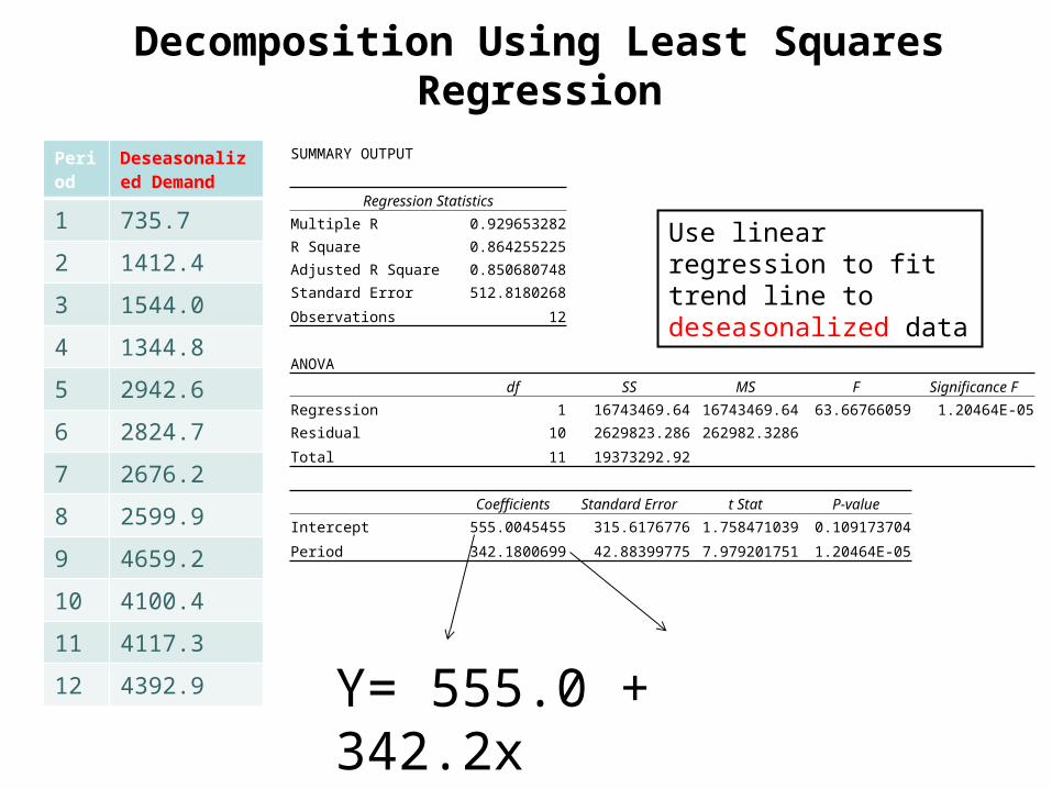
Decomposition Using Least Squares Regression

Period

Deseasonalized Demand

1 735.7

2 1412.4

3 1544.0

4 1344.8

5 2942.6

6 2824.7

7 2676.2

8 2599.9

9 4659.2

10 4100.4

11 4117.3

12 4392.9

SUMMARY OUTPUT

Regression Statistics

Multiple R 0.929653282

R Square 0.864255225

Adjusted R Square 0.850680748

Standard Error 512.8180268

Observations 12

ANOVA

  df SS MS F Significance F

Regression 1 16743469.64 16743469.64 63.66766059 1.20464E-05

Residual 10 2629823.286 262982.3286

Total 11 19373292.92      

  Coefficients Standard Error t Stat P-value

Intercept 555.0045455 315.6176776 1.758471039 0.109173704

Period 342.1800699 42.88399775 7.979201751 1.20464E-05

Y= 555.0 + 342.2x

Use linear regression to fit trend line to deseasonalized data

Create Forecast by Projecting Trend and Reseasonalizing

Period Quarter Y from Regression Seasonal Factor

Forecast

13 I 555+342.2*13=5003.5 X 0.82 = 4102.87

14 II 555+342.2*14=5345.7 X 1.10 = 5880.27

15 III 555+342.2*15=5687.9 X 0.97 = 5517.26

16 IV 555+342.2*16=6030.1 X 1.12 = 6753.71

Project Linear Trend Project Seasonality

Y= 555.0 + 342.2x

3.3. Short-term Forecasting Technique

Some basic concepts: dependent/independent demand aggregate/disaggregate demand long-term/short-term forecast (regression and correlation vs.

smoothing out the random fluctuations)

The underlying assumption of time series models is that the future values of the time series can be predicted based upon previous time series values (i.e., past conditions that produced the historical data won’t change !)

The need for some forecasting techniques (Fig. 3.11)

What’s wrong with drawing a line (i.e., use the regular averaging process)?

3.3. Short-term Forecasting Techniques

Moving Average:

Q: what n to use? large or small (longer or shorter)?

Q: Drawback of (simple) moving average?

Weighted Moving Average:

Example. Use weighted moving average with weights of 0.1, 0.2, and 0.3 to forecast demand for period 33.

Sol:

3.3. Short-term Forecasting Techniques

Exponential Smoothing Forecasting (ESF):

ESFt = ESFt-1 + α(actual demand t – ESFt-1) …….. (3.6)

=α(actual demand t ) + (1- α) ESFt-1 …….. (3.7)

where:α= the proportion of the forecast error, under or over estimate, that will be

incorporated into (next) forecast (i.e., smoothing constant).

ESFt-1 = Exp. smoothing forecast made at the end of period t-1 = Exp. smoothing forecast for period t

3.3. Short-term Forecasting Techniques

Exponential Smoothing Forecasting (ESF):

Q: Why is it called “exponential” smoothing? Proof

Q: What happens when α=0 or α=1?

Q: what αvalue to use? Small or large and the effects.

3.3. Short-term Forecasting Techniques

Bias = Σ(actual demand i – forecast demand i) /n

Bias (mean error) measures consistently high or low forecast

MAD = Σ|actual demand i – forecast demand i| /n

MSE= MAD (mean absolute deviation) measures the magnitude of

forecast error

What is a good (ideal) forecast? Which (Bias or MAD) is more critical? When the forecast errors are normally distributed, the standard

deviation of forecast errors = 1.25 MAD

3.3. Some Insights

Focus forecasting: uses the one forecasting model that would have performed the best in the recent past to make the next forecast.

Simple models usually outperform more complex methods, especially for short-term forecasting.

There is no one model that would consistently outperform all the others.

It might be a good idea to average the forecasts from several models used in each period (combination technique).

3.4. Using the Forecasts

Aggregating Forecasts:

Long-term or product-line forecasts are more accurate than short-term or detailed forecasts.

Theorem: Suppose that X and Y are independent random variables with normal distribution N(μ1 , σ1

2 ) and N(μ2 , σ22 ),

respectively. Let Z=X + Y, then Z is a normal distribution N(μ1+ μ2 ,σ1

2 +σ22 ).

Application: Figure 3.17

3.4. Using the Forecasts

Pyramid Forecasting:

To coordinate, integrate, and assure (force) consistency between forecasts prepared in different parts/levels of the organization and company goals or constraints. Figs. 18~20.

Incorporating External Information:

Change the forecast directly, if we know the activities that will influence demand for sure. e.g., promotions, product changes, competitor’s action, etc.

Change the forecast model, if we are not sure of the impact of the activities. e.g., use larger α to be more

responsive to demand change.