3. Defect equilibria...3. Defect equilibria 3.2 very practical laboratories or process containers...
32
3. Defect equilibria 3.1 3. Defect equilibria Introduction After having learned to formulate defect reactions in a compound, we now turn our interest towards the equilibrium relations for those reactions. These correlate the equilibrium concentrations of the different defects with temperature, activities (e.g. partial pressures) of the components in the compound, and other parameters which affect the defect structure. From a thermodynamic point of view a solid containing point defects constitutes a solid solution where the point defects are dissolved in the solid. In analogy with liquid solutions the solid may be considered to be the solvent and the point defects the solute. Thus, the defect equilibria may be treated in terms of the thermodynamics of chemical reactions and solutions. As examples of defect equilibria, mostly known from the preceding chapter, we may use the formation of a vacancy in an elemental solid; E E E E v E + = or the formation of a Schottky pair in MO, that we here choose to write; x O x M O M x O x M O M v v O M + + + = + • • // or the excitation of electronic defects, that we here choose to write; / e h e x + = • or the formation of oxygen deficiency; ) ( 2 2 2 1 / g O e v O O x O + + = • • From any starting point (given concentrations of reactants and products), a reaction may proceed to the right (forward) or left (backward). The proceeding of a reaction in some direction will be accompanied by changes in the internal energy U of the system. The change is called ΔU. At constant pressure (which we most normally consider) the change in energy is given by the change in enthalpy, H; ΔH. There will also be a change in the disorder (chaos) of the system, expressed by the entropy S. The entropy change is denoted ΔS. The first and second law of thermodynamics state that in an isolated system 3 the energy is constant and the entropy can only increase or remain constant. These laws are empirical – we cannot prove them, just experience them. Equilibrium thermodynamics in closed systems – that we shall now consider – is one such experience. The isolated system of the Universe or a closed thermobottle are not 3 An isolated system is a system that exchanges neither mass nor heat with its surroundings. The Universe is believed to be such a system. A closed insulated thermobottle is a good example of a practically isolated system.
Transcript of 3. Defect equilibria...3. Defect equilibria 3.2 very practical laboratories or process containers...
3. Defect equilibria
3.1
3. Defect equilibria
Introduction
After having learned to formulate defect reactions in a compound, we now
turn our interest towards the equilibrium relations for those reactions. These
correlate the equilibrium concentrations of the different defects with temperature,
activities (e.g. partial pressures) of the components in the compound, and other
parameters which affect the defect structure. From a thermodynamic point of view
a solid containing point defects constitutes a solid solution where the point defects
are dissolved in the solid. In analogy with liquid solutions the solid may be
considered to be the solvent and the point defects the solute. Thus, the defect
equilibria may be treated in terms of the thermodynamics of chemical reactions
and solutions.
As examples of defect equilibria, mostly known from the preceding
chapter, we may use the formation of a vacancy in an elemental solid;
EEE EvE +=
or the formation of a Schottky pair in MO, that we here choose to write;
x
O
x
MOM
x
O
x
M OMvvOM +++=+ ••//
or the excitation of electronic defects, that we here choose to write;
/ehe
x += •
or the formation of oxygen deficiency;
)(2 221/
gOevO O
x
O ++= ••
From any starting point (given concentrations of reactants and products), a
reaction may proceed to the right (forward) or left (backward). The proceeding of
a reaction in some direction will be accompanied by changes in the internal
energy U of the system. The change is called ∆U. At constant pressure (which we
most normally consider) the change in energy is given by the change in enthalpy,
H; ∆H. There will also be a change in the disorder (chaos) of the system,
expressed by the entropy S. The entropy change is denoted ∆S.
The first and second law of thermodynamics state that in an isolated system3
the energy is constant and the entropy can only increase or remain constant. These
laws are empirical – we cannot prove them, just experience them. Equilibrium
thermodynamics in closed systems – that we shall now consider – is one such
experience. The isolated system of the Universe or a closed thermobottle are not
3 An isolated system is a system that exchanges neither mass nor heat with its surroundings.
The Universe is believed to be such a system. A closed insulated thermobottle is a good example
of a practically isolated system.
3. Defect equilibria
3.2
very practical laboratories or process containers for our purpose. We want to
consider a closed system4, i.e. one that keeps the chemicals inside but exchanges
heat. From a textbook in thermodynamics you may learn how the 1st and 2
nd laws
of thermodynamics predict that any process or reaction in a closed system will
proceed spontaneously (voluntarily) only as long as T∆S > ∆H, that is, as long as
∆H -T∆S <0. You may say that the effect of disorder must overcome the energy
cost in the closed system for the process to run by itself.
For this purpose we see that the enthalpy H of a system can be split into
Gibbs (free) energy G and the energy given by the entropy and temperature: H =
G + TS. The change in the Gibbs (free) energy by a chemical reaction is thus
given by
TdSdHdG −= (3.1)
and, as stated above, a reaction proceeds as long as dG < 0. If dG > 0, it will
proceed backwards to make dG < 0. A reaction reaches equilibrium at dG = 0.
This extremely important conclusion we can use to understand and calculate
chemical equilibria.5
A reaction at equilibrium does in fact not mean that it has stopped, but that
the forward and backward reactions run equally fast. We will later on consider
equilibrium thermodynamics also from the viewpoint of the mass-action. This will
allow us to use the equilibrium constant, the main new tool of this chapter, plus
provide more insight to help understand chemical equilibrium.
The creation of single, unassociated point defects in an elemental,
crystalline solid increases the internal energy of the system and the enthalpy of the
defect formation is positive. But the configurational entropy of the system also
increases, and the equilibrium concentration of the defects will be reached when
the Gibbs energy of the system is at minimum. Thermodynamically, point defects
will thus always be present in a crystal above 0 K.
All types of defects will in principle be formed. However, the free energies
of formation of the different types and systems of defects can have widely
different values, and correspondingly it is often found that certain defects
predominate in a particular solid. The relative concentrations of the different types
of defects will be a function a temperature and other variables. Thus, defect
equilibria with large positive enthalpy of formation, for instance, which are not
favoured at low temperatures, may become important at high temperatures.
4 A closed system is one where the mass (chemical entities) of the system is confined, but
where energy (heat) can be exchanged with the surroundings. The expression for the Gibbs energy
arises as a result of the definition of entropy and of the first law of thermodynamics which
preserves the total energy of the system and the surroundings.
5 It has been said that chemists have the ability to accept its applicability and to use it for a
lifetime often without ever really understanding its derivation or basics. My experience is that
physicists have the tendency to reject it and to be unable to use it for the same reasons.
3. Defect equilibria
3.3
Point defects and equilibrium in an elemental solid - a simple statistical thermodynamic approach
Before considering the thermodynamics of defect formation and of defect
reactions in compounds such as metal oxides and the corresponding use of the law
of mass action, the simpler case of formation of one type of defect in an elemental
solid will be treated by means of statistical thermodynamics.
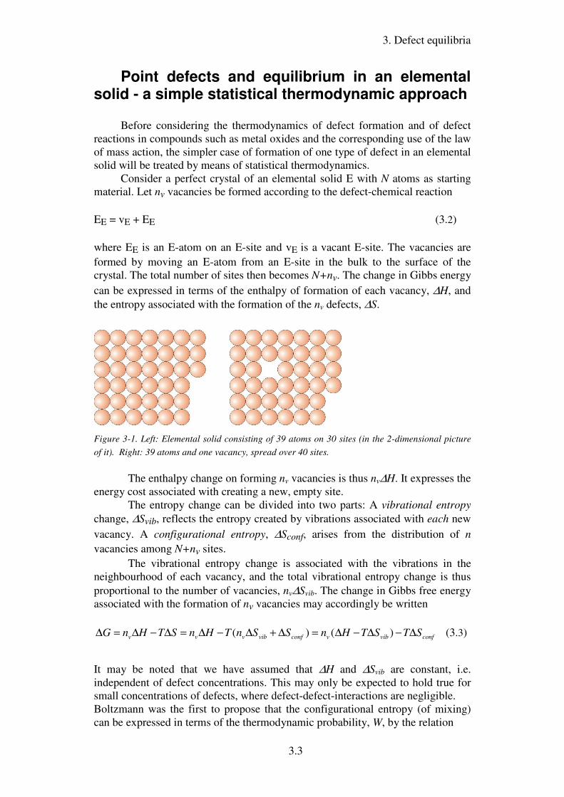
Consider a perfect crystal of an elemental solid E with N atoms as starting
material. Let nv vacancies be formed according to the defect-chemical reaction
EE = vE + EE (3.2)
where EE is an E-atom on an E-site and vE is a vacant E-site. The vacancies are
formed by moving an E-atom from an E-site in the bulk to the surface of the
crystal. The total number of sites then becomes N+nv. The change in Gibbs energy
can be expressed in terms of the enthalpy of formation of each vacancy, ∆H, and
the entropy associated with the formation of the nv defects, ∆S.
Figure 3-1. Left: Elemental solid consisting of 39 atoms on 30 sites (in the 2-dimensional picture
of it). Right: 39 atoms and one vacancy, spread over 40 sites.
The enthalpy change on forming nv vacancies is thus nv∆H. It expresses the
energy cost associated with creating a new, empty site.
The entropy change can be divided into two parts: A vibrational entropy
change, ∆Svib, reflects the entropy created by vibrations associated with each new
vacancy. A configurational entropy, ∆Sconf, arises from the distribution of n
vacancies among N+nv sites.
The vibrational entropy change is associated with the vibrations in the
neighbourhood of each vacancy, and the total vibrational entropy change is thus
proportional to the number of vacancies, nv∆Svib. The change in Gibbs free energy
associated with the formation of nv vacancies may accordingly be written
confvibvconfvibvvv STSTHnSSnTHnSTHnG ∆−∆−∆=∆+∆−∆=∆−∆=∆ )()( (3.3)
It may be noted that we have assumed that ∆H and ∆Svib are constant, i.e.
independent of defect concentrations. This may only be expected to hold true for
small concentrations of defects, where defect-defect-interactions are negligible.
Boltzmann was the first to propose that the configurational entropy (of mixing)
can be expressed in terms of the thermodynamic probability, W, by the relation

3. Defect equilibria
3.4
WkSconf ln= (3.4)
where k is Boltzmann's constant. The thermodynamic probability W represents in
this case the number of distinguishable ways whereby nv vacancies may be
distributed on N+nv lattice sites and is given as
!!
)!(
v
v
nN
nNW
+= (3.5)
We recognise that for the perfect crystal nv=0 so that W=1 and Sconf=0. As the
number of vacancies increases, Sconf increases and we have ∆Sconf= Sconf.
For large numbers of N and nv, which is typical for real crystals, Stirling's
approximation ( xxxx −= ln!ln for x>>1) may be applied, whereby Eq. (3.5)
takes the form
)lnln(v
vv
vconf
n
nNn
N
nNNkS
++
+=∆ (3.6)
By insertion into the expression for the change in free energy Eq. (3.3) we get
)lnln()(v
vv
vvibvv
n
nNn
N
nNNkTSTHnG
++
+−∆−∆=∆ (3.7)
The changes in enthalpy, entropy, and Gibbs energy are illustrated in Figure 3-2.
Figure 3-2. Example of the variation in enthalpy, vibrational and configurational entropy, and
Gibbs energy with the concentration of vacancies in an elemental solid.
3. Defect equilibria
3.5
At equilibrium G and thus ∆G will be at a minimum with respect to nv , i.e.
d∆G/dnv = 0;
0ln G
=+
+∆−=v
vvib
V nN
nkTST∆H
dn
d∆ (3.8)
The term nN
n
v
v
+ represents the fraction of the total number of sites which are
vacant and is through rearrangement given by
)kT
∆H()
k
∆S(
nN
n vib
v
v −=
+expexp (3.9)
Since the formation of the vacancies is written EE = vE + EE, the equilibrium
constant may, following the law of mass action, be written
)kT
∆H()
k
∆S(
nN
n XaK vib
v
vvv EE
−=
+=== expexp (3.10)
Eva is the activity and nN
n X
v
vvE +
= represents the site fraction of vacancies in
the crystal.
∆Svib in the expressions above represents the vibrational entropy change
and ∆H the enthalpy change per vacancy. If one wants to express the same
properties per mole of vacancies, k must be substituted by the gas constant R =
NAk where NA is Avogadro's number. Relations corresponding to Eq. (3.10) may
be derived for other types of point defects.
At any temperature T>0 all solids will following Eq. (3.10) contain point
defects. In the example above we have shown that the equilibrium constant,
containing defect activities as site fractions, is given by an enthalpy change and an
entropy term which constitutes the vibrational entropy change as one goes from
the reactants to the products. It does not contain the (configurational) entropy
change.
This applies to chemical reactions and their equilibrium constants in
general. Furthermore, it illustrates that the vibrational entropy change enters
without other contributions if the equilibrium constant is expressed properly, as
activities. Each activity is unitless, that is, it is some concentration divided by the
concentration in the standard, reference state. For defects, activities are given as
site fractions. When activities properly use standard states as reference, the
enthalpy and vibrational entropy changes are called standard enthalpy and entropy
changes, ∆H0 and ∆S
0, respectively.
We may combine the standard enthalpy and entropy changes into a
standard Gibbs energy change:
)RT
∆G()
RT
∆H()
R
∆S( K vib
000
expexpexp−
=−
= (3.11)
3. Defect equilibria
3.6
We will see later that this standard Gibbs energy change is the Gibbs energy
change we have when the reaction proceeds with all reactants and products in their
standard reference state (activity of unity). It is not the same as the variable Gibbs
energy change calculated for the progression of the defect formation reaction
earlier.
What happened to the configurational entropy? Should it not be part of the
entropy that balances the reaction at equilibrium? And what is K? Look at Eq.
(3.11). The right hand side tells us via the standard enthalpy, entropy, and Gibbs
energy changes how much the reaction wants to proceed when all reactants and
products are in their standard states. If ∆G0 < 0 it is a favourable reaction. K is
the quotient of all product activities over all reactant activities when equilibrium is
attained. In other words, K tells us how much the activities have to deviate from
the standard state in order to balance the force from ∆G0
to drive the reaction
forward (∆G0<0,
K>1) or backward (∆G
0>0,
K<1). One may thus say that the
configurational entropy is in the K.
In our example of the elemental solid, the equilibrium quotient K
contained only the activity of the product, the site fraction of vacancies.
What were the standard states in our example? For atoms, it is a site
fraction of 1, i.e. the perfect crystal is the standard state. For the vacancies it is
also a site fraction of 1, i.e. an empty crystal! This exemplifies that standard states
of defects are virtual.
Thermodynamics of chemical reactions
As a basis for the subsequent considerations of thermodynamics of defect
equilibria the following section provides a brief review of some general aspects of
thermodynamics of chemical reactions.
In treating chemical reactions and systems consisting of two or more
constituents, it is convenient to introduce the concept of partial molar
thermodynamic quantities. As regards equilibria, the partial molar Gibbs energy is
particularly important. The partial molar Gibbs energy is commonly termed the
chemical potential and written µ i. The physical significance of a partial molar
property is the increase in the value of that property resulting from the addition of
1 mole of that constituent to such a large quantity of the system that its
composition remains essentially unchanged. If a system consists of n1 + n2 + ... +
ni moles of constituents 1, 2, …and i, the partial molar free energy for the "i"th
constituent is given by
)n
G( ,...,np,T,
i
i 21 n∂
∂µ = (3.12)
The Gibbs energy of a system is in terms of chemical potentials of the
constituents given by
.... i2211 µµµ innnG ++= (3.13)
3. Defect equilibria
3.7
When a chemical reaction takes place, the numbers of various constituents change,
and dG changes correspondingly. For an open system (i.e. where we may add or
remove heat and mass) at constant temperature and pressure, dG is given by
.... i2211, ipT dndndndG µµµ ++= (3.14)
At equilibrium we have
0i, ==∑i
ipT dndG µ (3.15)
It may also be shown that under equilibrium conditions
0 .... i2211 =++ µµµ dndndn i (3.16)
This equation is one form of the Gibbs-Duhem equation.
In a chemical reaction , e.g.
dDcCbBaA +=+ (3.17)
the change in Gibbs energy is given by the difference in the total free energy in
the final and initial state
)( BADC badcG µµµµ +−+=∆ (3.18)
The chemical potential of the constituent "i" in the mixture can be written
iii aRT ln0+= µµ (3.19)
where ai is the activity of constituent "i" in the mixture and 0
iµ is the chemical
potential of constituent "i" at a chosen standard state of unit activity.
The activity of pure solids or liquids is usually taken as unity at
atmospheric pressure (1 bar or 105 Pa), while for gases the activity is unity when
the partial pressure of the gas constituent is 1 bar.
In solutions the activity may be equated with the mole fraction, Xi, in ideal
solutions:
ii Xa = (3.20)
In non-ideal solutions the activity is related to the mole fraction through the
activity coefficient, γi,
iii Xa γ= (3.21)
3. Defect equilibria
3.8
γi is thus equal to unity in ideal solutions. It may be noted that in a system
consisting of several phases, the condition of equilibrium implies that the
chemical potential of constituent "i" is the same in all phases.
If one introduces the expression for the chemical potential in Eq. (3.19)
into Eq. (3.18) it follows that ∆G for the reaction in Eq. (3.17) is given by
b
B
a
A
d
D
c
C
aa
aaRTGG ln0 +∆=∆ (3.22)
where )( 00000
BADC badcG µµµµ +−+=∆ represents the change in Gibbs energy in
the standard state, i.e. at unit activities. ∆G° is a constant under specified standard
states. At equilibrium 0=∆G such that
mequilibriu
b
B
a
A
d
D
c
C
aa
aaRTG
−=∆ ln0 (3.23)
where the quotient at equilibrium is called the equilibrium coefficient, K:
Kaa
aa
mequilibriu
b
B
a
A
d
D
c
C =
(3.24)
K is termed the equilibrium coefficient as it relates the ratio of activities of
products and reactants when equilibrium has been attained at a given temperature.
It takes a constant value at any given temperature and is thus also often called the
equilibrium constant. ∆G° may as in Eq. (3.1) be expressed in terms of the
standard enthalpy change, ∆H°, and entropy change, ∆S°, such that
KRTSTHG ln000 −=∆−∆=∆ (3.25)
This may be rewritten in the form
)exp()exp()exp(000
0
RT
H
R
S
RT
HKK
∆−∆=
∆−= (3.26)
Thus, we have arrived at the same type of expression for the equilibrium constant
as we did in our intitial example from statistical thermodynamics. From that, we
know that the entropy term contained in K° = exp(∆S°/R) contains the change in
vibrational entropy terms between the reactants and products in their standard
states, and that it does not contain the configurational entropy change involved by
the system when the activities are different from the standard states.
From the equation above we see that the temperature dependence of K is
given by
3. Defect equilibria
3.9
R
H
Td
Kd0
)/1(
ln ∆−= (3.27)
and that a plot of lnK vs 1/T (van ’t Hoff plot) will give ∆S°/R as the intercept and
-∆H°/R as the slope.
This general treatment is applicable to any ideal solutions whether these
are gaseous, liquid, or solid, and it applies also to defect chemistry as we have
exemplified initially.
Thermodynamics and point defects
Equilibrium thermodynamics may as stated above be applied to defect
reactions. However, before so doing it is of interest to consider the
thermodynamic properties of the individual point defects.
Virtual chemical potentials of point defects
The regular atoms on their normal sites and the point defects occupy
particular sites in the crystal structure and these have been termed structural
elements by Kröger, Stieltjes, and Vink (1959) (see also Kröger (1964)). As
discussed in Chapter 2, the rules for writing defect reactions require that a definite
ratio of sites is maintained due to the restraint of the crystal structure of the
compounds. Thus if a normal site of one of the constituents in a binary compound
MO is created or annihilated, a normal site of the other constituent must
simultaneously be created or annihilated.
As discussed above the chemical potential of a constituent represents the
differential of the Gibbs energy with respect to the amount of the constituent when
the pressure, temperature and the amounts of all other constituents are kept
constant. When a structure element is created, the number of complementary
structure elements can not be kept constant due to the requirement of a definite
site ratio, and it is therefore not possible to assign a true chemical potential to a
structure element. However, Kröger et al. showed that one may get around this
difficulty by assigning a virtual chemical potential ζ (zeta) to each separate
structure element and that the virtual chemical potential behaves like a true
chemical potential and may be related in a similar way to activity:
iii aRT ln0+= ζζ (3.28)
The virtual potential differs from the true chemical potential by an undefined
constant which is incorporated in ζ°. For this reason the absolute value of the
virtual chemical potential can not be determined experimentally.
In real changes in crystals where the site ratio is maintained and
complementary structure elements (or building units) are created or annihilated,
the undefined constants in the virtual chemical potential of each separate structure
element cancel out, and the overall change is characterised by real changes in
3. Defect equilibria
3.10
Gibbs free energies; dGi = dµi = dζi = dRTlnai. At constant temperature and with
ideal conditions (small concentrations of defects), a change in activity corresponds
to the change in concentration, and we have dGi = dµi = RTdlnai = RTdln(ci/c0) =
RTdlnci.
Kröger et al. pointed out that a similar treatment applies to aqueous
electrolytes.
As we have mentioned before, we have not only the problem of measuring
true chemical potentials µ of defects and other structure elements, we also have
the problem of establishing or even imagining the standard state of site fraction of
unity: For oxygen vacancies in a simple oxide this would for instance mean a
crystal where all oxide ions are missing, i.e. a crystal with only cations.
Ideal and non-ideal models
As described in the preceding section the defect reactions and equilibria can
be described as chemical reactions and treated in terms of the law of mass action.
It is emphasised that the equilibrium constants relate activities of the structure
elements involved in the defect reaction, but under ideal conditions and when the
structure elements can be assumed to be randomly distributed over the available
sites, the activities equal the concentrations of the structure elements. This is a
valid assumption for very dilute solutions. However, for larger defect
concentrations interactions take place between the defects, etc. and in principle
activities should be used instead of concentrations.
The interactions between charged defects may be accounted for by using the
Debye-Hückel theory in analogy with the interactions of ions in aqueous
solutions. This requires knowledge of the relative dielectric constant, the smallest
distance between charged defects, and other parameters for the solid. Debye-
Hückel corrections have, for instance, been worked out and tested for cation
vacancy defects in metal-deficient Co1-xO and Ni1-xO. At infinite dilution the
metal vacancies can be considered to have two negative charges, //
Cov , and the
equivalent number of electron holes is assumed to be randomly distributed in the
oxide. With an increasing concentration of point defects and electron holes, there
will be an increasing association of the metal vacancies (with two effective
negative charges) and the positively charged electron holes. In these terms, the
metal vacancies can be considered surrounded by a cloud of electron holes. This
results in a deviation from a random distribution of electron holes and a
corresponding deviation from the ideal solution model. For the case of Co1-xO the
Debye-Hückel correction can explain the increasing deviation from ideality with
increasing defect concentration. However, this model in its present form does not
satisfactorily explain various electrical conductivity results for Co1-xO and so far
apparently fails to give a full description of the defect structure and defect-
dependent properties of the oxide.
An alternative approach is to consider that the association of defects leads to
the formation of new "associated" defect species. These "new" defects are, in turn,
treated in terms of the ideal solution models. Specifically, in the case of metal
vacancies in, for instance, Co1-xO and Ni1-xO it is assumed that the metal

3. Defect equilibria
3.11
vacancies with two effective charges become associated with one electron hole to
give a metal vacancy with one negative effective charge, /
Cov , as has already been
described in Chapter 2. At this stage this simple approach appears to give an
equally consistent description of the defect structure and defect-dependent
properties of Co1-xO as the much more complicated Debye-Hückel model.
However, it is to be expected that future developments will provide a more
detailed understanding of defect interactions and how they influence defect-
dependent properties of inorganic compounds.
Despite its shortcomings the ideal solution approach will be used in this
book in treating defect equilibria. Defect interactions will generally be treated by
assuming the formation of associated defects as is, for instance, exemplified above
for the formation of singly charged metal vacancies through the association of an
electron hole with a doubly charged metal vacancy. Furthermore, the defect
equilibria will be treated using the law of mass action.
Concentrations of the structure elements may be expressed in many units. In
semiconductor physics it is common to express the concentrations in number per
cm3. This has the disadvantage, however, that when two compounds with different
molecular (packing) densities contain the same number of defects per cm3, the
number of defects per molecular unit is different in the two compounds, and vice
versa. Furthermore, the molecular unit size (packing density, or unit cell
parameters) of a compound changes as a function of its nonstoichiometry and
temperature, and in this case the unit of defects per cm3 does not unequivocally
reflect the relative defect concentration per molecular unit or atom site under
different conditions.
In the following, concentration will in most cases be expressed as the
number of defects or atoms per molecular unit or site, i.e. in molar or site
fractions, while we for some purposes need to use the number of defects per cm3.
As mentioned before, the value of the equilibrium constant depends on the units of
concentration that are employed, but it is a simple matter to convert the values of
the equilibrium constant from one system to another.
Examples of defect equilibria in pure, stoichiometric metal oxides
In this section we will see how we write defect reactions for selected simple
cases of combinations of defects, express the equilibrium constants, and combine
this with an electroneutrality condition to express the concentration of dominating
defects as a function of temperature and activities. We will when possible stay
with proper statistical thermodynamics, such that entropy changes in the defect
reaction can be interpreted as a change in the vibrational entropy from reactants to
products in their standard states. Approximations will be implemented in order to
visualise the simplicity of the method.
3. Defect equilibria
3.12
Schottky defects
As a first illustration let us consider the defect equilibrium for Schottky
defects in the oxide MO and where the metal and oxygen vacancies are doubly
charged. The defect equation for their formation is given in Chapter 2 as
//0 MO vv += •• (3.29)
The corresponding defect equilibrium may at low defect concentrations be written
[M]
][
[O]
][XX
//
//
MO
vvS
vvK
MO
••
== •• (3.30)
where KS is the equilibrium constant for a Schottky defect pair, X represent site
fractions, and square brackets express concentrations of species. [O] and [M]
represent the concentration of oxygen and metal sites, respectively.
If we let square brackets express concentration in mole fraction (i.e. the
number of moles of the species per mole of MO), then [O] = [M] = 1, and then
]][[ //
MOS vvK••= (3.31)
When the concentrations of the defects are expressed in site fractions, or
properly converted to mole fractions as here, KS is related to the standard Gibbs
energy cange ∆GS0, enthalpy change ∆HS
0, and entropy change ∆SS
0, of formation
of pairs of doubly charged Schottky defects:
)RT
∆H(-)
R
∆S()
RT
∆G(-vvK SSS
MOS
000// expexpexp ]][[ === •• (3.32)
It may be useful to repeat that the entropy change ∆SS0 does not include the
configurational entropy changes associated with the formation of the defects, but
only the change in vibrational entropy associated with the vacancies formed.
When the Schottky pair dominates the defect structure, we may see from
the reaction equation or from the electroneutrality condition that in MO the
concentrations of the metal and oxygen vacancies are equal:
][][ //
MO vv =•• (3.33)
Insertion into the preceding equation yields
)RT
∆H()
R
∆S(Kvv SS
MO2
exp2
exp ][][00
2/1
S
// −===•• (3.34)
Under these conditions the defect concentrations are only dependent on the
temperature; they are independent of the activities of the components M and O2.
The slope in a van ’t Hoff plot of ]ln[ ••Ov or ]ln[ //
Mv vs 1/T would be -∆HS0/2R, see

3. Defect equilibria
3.13
Figure 3-3. The factor 2 results from the square root of the equilibrium constant,
in turn resulting from the fact that there are two defects created, in comparison
with the one we got in the element used as example earlier.
Figure 3-3. van ’t Hoff plot of the logarithm of defect concentrations vs inverse absolute
temperature yields intercept and slope related to the standard entropy and enthalpy, respectively,
of the defect formation reaction, divided by the number of defects formed and R.
It may be useful to note that the procedure we have applied is to write
down the defect reaction and the mass action law expression for its equilibrium
constant, and the prevailing electroneutrality condition. Thus, we have two
independent equations for the two unknowns (provided that either KS or all of
∆SS0, ∆HS
0, and T are known).
Frenkel defect pairs
In our next example we consider Frenkel defect pairs in MO. If, for the sake
of illustration, the Frenkel defects in MO are assumed to be doubly charged, the
defect equation for their formation is given as
••+=+ iM
x
i
x
M MvvM// (3.35)
It may be noted that a vacant interstitial site has been included to keep track of the
sites where the interstitials are going. The corresponding defect equilibrium is
written as
]][[
]][[
][
][
][
][
[i]
][
][
][//
//
x
i
x
M
iM
x
i
x
M
iM
vM
Mv
FvM
Mv
i
v
M
M
M
M
v
XX
XXK
xi
xM
i//M
••
••
===••
(3.36)
If there is one interstitial site per MO, and if the defect concentrations are small
such that 1 ][][ == x
i
x
M vM , we obtain simply
]][[ //
MiF vMK••= (3.37)
3. Defect equilibria
3.14
If Frenkel defects predominate in the pure stoichiometric compound, the
concentrations of interstitial cation and vacancies are then equal, and we obtain:
)RT
H-()
R
∆S(KvM FF
Mi2
exp2
exp ][][00
2/1
F
// ∆===•• (3.38)
where ∆SF0 and ∆HF
0 are the standard entropy and enthalpy changes of formation
of Frenkel defect pairs. Under these conditions the concentration of the Frenkel
defect pairs is independent of the activities of the metal and oxygen components.
Intrinsic ionisation of electrons
For many oxides, and particularly when considering defect structure
situations close to stoichiometry, it is essential to take into account the intrinsic
ionisation of electrons. This can include localised defects (valence defects) or
delocalised defects (valence band and conduction band).
In the case of valence defects, the ionisation of a pure binary metal oxide
MaOb may typically be assigned to mixed valency of the metal and thus be written
as
•+= MM
x
M MMM /2 (3.39)
The equilibrium constant may then be expressed as site fractions, which in our
case immediately simplifies into an expression containing only volume or molar
concentrations:
][
]][[2
/
x
M
MMi
M
MMK
•
= (3.40)
If this intrinsic ionisation dominates the defect structure, we have
][][ /
MM MM =• (3.41)
Insertion into the equilibrium constant yields
)2RT
exp()2R
]exp([][][][00
21/ iix
M
/
i
x
MMM
HSMKMMM
∆−∆===• (3.42)
In the case of delocalised electrons we write the ionisation reaction
•+= he0 / (3.43)
If we describe this as a chemical reaction, the product of the activities of the
electrons and holes should remain constant at a given temperature. However,

3. Defect equilibria
3.15
electrons and holes in the band model do not occupy sites, but energy states, and
thus the activity might be represented as the fraction of concentration over density
of states:
VCVC
/
heiN
p
N
n
N
][h
N
][eaaK / ===
•
• (3.44)
where iK is the equilibrium coefficient and n and p denote the concentrations of
electrons and holes, respectively. NC and NV denote the density of states in the
conduction band and valence band edges, respectively. If we apply statistical
thermodynamics to this we might assign Ki to standard Gibbs energy, entropy and
enthalpy changes:
RT
H
R
S
RT
HK
RT
G
N
p
N
nK iii
ii
VC
i
000
,0
0
expexpexpexp∆−∆
=∆−
=∆−
== (3.45)
However, the use of entropy is not commonly adopted for reactions involving
band electrons and holes, as the concept of the standard states, that would imply
n=NC and p=NV, are not commonly accepted. In physics, one instead uses simply6
RT
ENNn pheK
g
VC
/
i
−=== • exp]][[ / (3.46)
where Eg is the band gap. We see from this that iVC
/
i KNNK = and that the band
gap would correspond to the standard Gibbs energy change of the intrinsic
ionisation reaction. The prime on this /
iK and others to follow is used here
to denote an equilibrium coefficient that has been multiplied with densities
of state such that it gets units (e.g. m-6
or cm-6
as here) and cannot be
directly related to an entropy.
Our brief discussion of electronic ionisation as seen from both defect
chemical and physics perspectives may seem confusing, and is in fact not
well resolved in textbooks or in the literature. This should not prevent us
from coming out with a simple conclusion: The product np is constant at
any given temperature, and its variation with temperature is roughly given
by the band gap, Eg.
If the concentrations of electrons and electron holes predominate, then the
electroneutrality condition is n = p and insertion into the equilibrium coefficient
yields
6 Physicists mostly use Eg/kT with Eg in eV per electron, while chemists often use Eg/RT (or
∆G0/RT) with Eg in J per mole electrons. This is a trivial conversion (factor 1 eV = 96485 J/mol =
96.485 kJ/mol).

3. Defect equilibria
3.16
)RT
E(NN)(Kpn
g
VC
//
i2
exp)( 2/121−
=== (3.47)
The density of states is often – under certain assumptions – approximated as
2/3
2
*8
=
h
kTmN e
C
π and
2/3
2
*8
=
h
kTmN h
V
π (3.48)
where the constants have their usual meanings, and *
em and *
hm are the effective
masses of electrons and holes, respectively. Effective masses are sometimes
known, or may be to a first approximation be set equal to the rest mass of
electrons, whereby NC and NV may be estimated. It may be noted that they
have units of m-3
and that they contain temperature dependencies of T3/2
. Intrinsic ionization of electrons and holes is, for instance, concluded to
dominate the defect structure of Fe2O3 and Cr2O3 at high temperatures.
Defect equilibria in nonstoichiometric oxides
Here, we will employ mainly the same methodology as in the preceding
section, but when delocalised defect electrons and holes are introduced we cannot
stay strictly with statistical thermodynamics and the equilibrium thermodynamics
cannot be related in the same simple manner to the change in vibrational entropy
any longer.
Oxygen deficient oxides
In oxides with oxygen deficit, the predominant defects are oxygen
vacancies. If these are fully ionised (doubly charged), and if the electronic defects
are localised as valency defects, their formation reaction can be written:
)(22 221/
gOMvMO MO
x
M
x
O ++=+ •• (3.49)
The corresponding equilibrium coefficient shall be expressed in terms of
activities. Writing these as site fractions for the defects, and as partial pressure for
the gas species (the division by the standard state of 1 bar is omitted for
simplicity) we get
2/1
2
2/
2/1
2
2
22
/
]][[
]][[Ox
M
x
O
MO
O
MO
Mv
vO pMO
Mvp
XX
XXK
xM
xO
MO
••
==••
(3.50)
3. Defect equilibria
3.17
If these oxygen vacancies and the compensating electronic valence defects are the
predominating defects in the oxygen deficient oxide, the principle of
electroneutrality requires that
]2[ ][ / ••= OM vM (3.51)
By insertion, and assuming the oxide is MO and that 1][][ == x
O
x
M OM (small
defect concentrations) we then obtain:
6100
316131/
22 3exp
3exp22 ]2[v][M /
OvOvO//
O
/
vOOM )pRT
∆H()
R
∆S(p)K(
−−•• −=== (3.52)
This shows that the concentrations of the dominating defects (defect electrons and
oxygen vacancies) increase with decreasing oxygen partial pressure. It
furthermore shows the relation between defect concentrations and entropy and
enthalpy changes of the defect reaction. The factor 3 that enters results from the
formation of 3 defects in the defect reaction.
Now, let us do the same treatment, but for an oxide where defect electrons
are delocalised in the conduction band. The formation of oxygen vacancies is then
written:
)(2 221/
gOevO O
x
O ++= •• (3.53)
The equilibrium coefficient should be
2/1
0
2
C
2/1
0
2
C
2/1
)(
2
2
22
2
2/
N
n
][
][
][
][
N
n
][
][
=
==••
••
••
O
O
x
O
O
x
O
O
OO
O
gOev
vOp
p
O
v
O
O
p
p
O
v
a
aaaK
xO
O (3.54)
It is common for most purposes to neglect the division by NC, to assume 1][ =x
OO
and to remove 10
2=Op bar, so that we get
2/12/
2]n[ OOvO pvK
••= (3.55)
This means that vOCvO KNK2/ = and that the expression is valid for small
concentratuons of defects.
If these oxygen vacancies and the compensating electrons are the
predominating defects in the oxygen deficient oxide, the principle of
electroneutrality requires that
]2[ n ••= Ov (3.56)
By insertion we then obtain:
3. Defect equilibria
3.18
610
31
0
6131
22 3exp222 /
OvO//
,vO
/
O
//
vOO )pRT
∆H(-)K(p)K(] [vn
−−•• === (3.57)
and deliberately use a pre-exponential K0/ instead of an entropy change.
Otherwise, the solution is the same as in the case with localised valence defects
for the electrons.
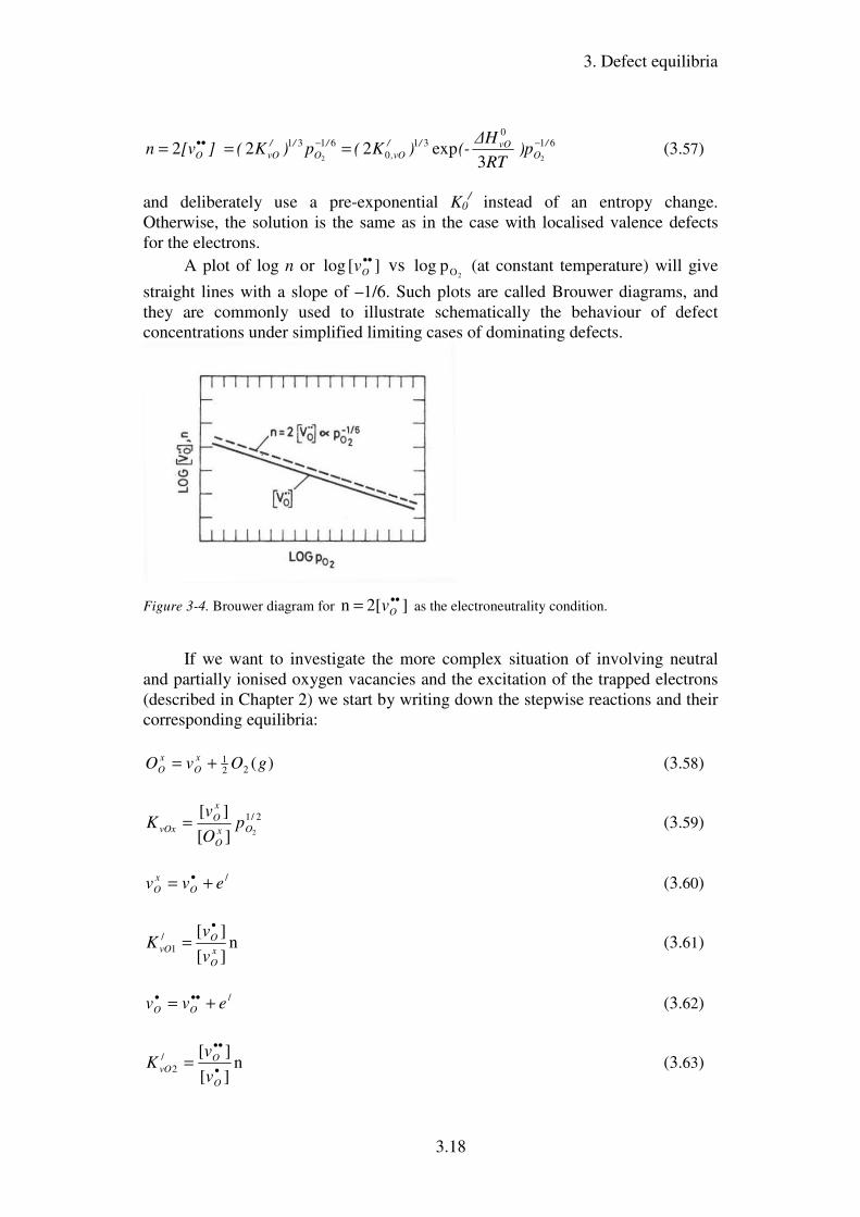
A plot of log n or ][ log ••Ov vs
2Op log (at constant temperature) will give
straight lines with a slope of –1/6. Such plots are called Brouwer diagrams, and
they are commonly used to illustrate schematically the behaviour of defect
concentrations under simplified limiting cases of dominating defects.
Figure 3-4. Brouwer diagram for ]2[ n ••= Ov as the electroneutrality condition.
If we want to investigate the more complex situation of involving neutral
and partially ionised oxygen vacancies and the excitation of the trapped electrons
(described in Chapter 2) we start by writing down the stepwise reactions and their
corresponding equilibria:
)(221 gOvO
x
O
x
O += (3.58)
2/1
2][
][Ox
O
x
O
vOx pO
vK = (3.59)
/
evv O
x
O += • (3.60)
n][
][/
1 x
O
O
vOv
vK
•
= (3.61)
/
evv OO += ••• (3.62)
n][
][/
2 •
••
=O
O
vOv
vK (3.63)

3. Defect equilibria
3.19
where /
2
/
1 and ,, vOvOvOx KKK are the respective equilibrium constants. Now the
principle of electroneutrality requires that
]2[ ][n ••• += OO vv (3.64)
The concentrations of the electrons and the neutral, singly, and doubly charged
oxygen vacancies are related through the equations above, and by combination
expressions for each of the defects may be obtained. The electron concentration is
given by
2/1/
2
/
1
3
2)2( −+= OvOvOvOx pnKKKn (3.65)
This equation has two limiting conditions.
If /
22
vOKn << , then
6/13/1/
2
/
1 2)2(][2 −•• == OvOvOvOxO pKKKvn (3.66)
Under these conditions the concentrations of electrons and oxygen vacancies are
relatively small, the doubly charged vacancies are the predominating oxygen
vacancies, and the concentrations of electrons and these oxygen vacancies are
proportional to 6/1
2
−Op . Of course, this situation corresponds to the simple case
presented initially for the doubly charged vacancies, and obviously //
2
/
2 vOvOvOvOx KKKK = .
If, on the other hand, /
22
vOKn >> , then
4/12/1/
1 2)(][ −• == OvOvOxO pKKvn (3.67)
Under these conditions the concentration of electrons is relatively large, and the
predominant oxygen vacancies are then singly charged. Furthermore, the
concentrations of electrons and oxygen vacancies are then proportional to 4/1
2
−Op .
A general tendency similar to that of oxygen deficient oxides applies to
metal deficient oxides; in the oxide M1-xO the metal vacancies are doubly charged
at very small deviations from stoichiometry and tend to become singly charged
with increasing nonstoichiometry.
It may be noted that the neutral oxygen vacancies are not affected by
charged defects, nor do they affect the electroneutrality.
Oxide with excess metal
We will as an example consider the formation of fully ionised interstitial
metal ions and complementary electrons in an oxide with excess metal M2+xO3.
The equation for the formation of interstitial metal ions with three effective
positive charges and three complementary electrons is given by
3. Defect equilibria
3.20
)(3 243/
23 gOeMMO i
x
M
x
O ++=+ ••• (3.68)
The corresponding defect equilibrium is given by
-1-3/24/33/ ][][]n[
2
x
M
x
OOiMi MOpMK•••= (3.69)
where K/Mi is the equilibrium constant. If these defects are the predominating
ones, and we as before assume small defect concentrations, the electroneutrality
condition and the oxygen pressure dependence of the interstitial metal ions and the
electrons is
16/34/1/
2)3(n]3[ −••• == OMii pKM (3.70)
Thus, also in this case the concentration of the defects increases with decreasing
oxygen activity and is now proportional to -3/16
O2p . This oxygen pressure
dependence is different from that for formation of singly as well as doubly
charged oxygen vacancies. In such a case it would thus in principle be possible to
decide from measurements of electron concentration (e.g. via electrical
conductivity) or of nonstoichiometry as a function of oxygen activity whether the
predominating defects are triply charged interstitial metal ions or oxygen
vacancies with one or two charges.
Had the metal interstitials predominantly been doubly charged in the oxide
M2+xO3, a -1/4
O2p dependence would have been the result, and additional studies of
defect-dependent properties (e.g. self-diffusion of metal or oxygen) would be
needed to distinguish this situation from that of singly charged oxygen vacancies.
It may be noted that it is not only the absolute number of charges on a
defect that determines the 2Op dependence, but also the difference between the
actual charge and the charge given by the nominal valence of the atoms involved.
Thus, in the oxide MO (or M1+xO) doubly charged metal interstitials will give a -1/6
O2p dependence of the defect concentrations (as opposed to the case above) and
in this case be indistinguishable from doubly charged oxygen vacancies.
Simultaneous presence of oxygen vacancies and interstitial metal ions
In an oxide MaOb where the ratio of metal to oxygen is larger than the
stoichiometric ratio a:b it is a priori difficult to predict whether interstitial metal
ions or oxygen vacancies predominate. In principle both types of defects may be
important, at least in certain regions of nonstoichiometry. In the following, let us
consider a case where it may be necessary to take into account the simultaneous
presence of interstitial metal ions and oxygen vacancies.
Consider an oxide with a stoichiometric composition MO2. Let us further
assume for the sake of illustration that when the oxide is nonstoichiometric the
important point defects are doubly charged oxygen vacancies and doubly charged
interstitial metal ions. (It may be noted that the metal interstitials are not fully

3. Defect equilibria
3.21
ionised in this case.) The composition of the nonstoichiometric oxide may
accordingly be written M1+yO2-y.
The defect equations for the formation of these two types of defects are
written
)(2 221/
gOevO O
x
O ++= •• (3.71)
)(22 2
/gOeMMO i
x
M
x
O ++=+ •• (3.72)
The corresponding defect equilibria (assuming [MM] and [OO] to be equal to
unity) then become
-12/12/ ][]n[
2
x
OOOvO OpvK••= (3.73)
-1-22/
2 ][][]n[2
x
M
x
OOiMi MOpMK••= (3.74)
The electroneutrality condition is given by
]2[][2 •••• += iO Mvn (3.75)
Two limiting conditions may be considered:
When ][][ •••• >> iO Mv then
6/13/1/
2)2(][2 −•• == OvOO pKvn (3.76)
as obtained also earlier for the same conditions. By inserting this relationship for n
into the equilibrium constant for formation of the minority defects, metal
interstitials, we obtain
3/23/2//
2 2)2(][ −−•• = OvOMii pKKM (3.77)
Under these conditions the minority concentration of metal interstitials, ][ ••iM ,
increases rapidly with decreasing oxygen partial pressure, more rapidly than the
two dominating defects, and may eventually catch up with them and become
dominating at the expense of oxygen vacancies, as illustrated in the figure below.
3. Defect equilibria
3.22
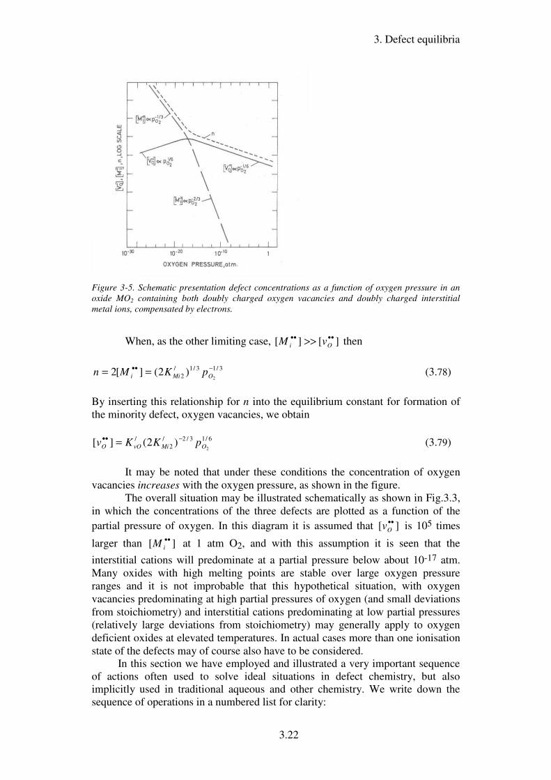
Figure 3-5. Schematic presentation defect concentrations as a function of oxygen pressure in an
oxide MO2 containing both doubly charged oxygen vacancies and doubly charged interstitial
metal ions, compensated by electrons.
When, as the other limiting case, ][][ •••• >> Oi vM then
3/13/1/
2 2)2(][2 −•• == OMii pKMn (3.78)
By inserting this relationship for n into the equilibrium constant for formation of
the minority defect, oxygen vacancies, we obtain
6/13/2/
2
/
2)2(][ OMivOO pKKv
−•• = (3.79)
It may be noted that under these conditions the concentration of oxygen
vacancies increases with the oxygen pressure, as shown in the figure.
The overall situation may be illustrated schematically as shown in Fig.3.3,
in which the concentrations of the three defects are plotted as a function of the
partial pressure of oxygen. In this diagram it is assumed that ][ ••Ov is 105 times
larger than ][ ••iM at 1 atm O2, and with this assumption it is seen that the
interstitial cations will predominate at a partial pressure below about 10-17 atm.
Many oxides with high melting points are stable over large oxygen pressure
ranges and it is not improbable that this hypothetical situation, with oxygen
vacancies predominating at high partial pressures of oxygen (and small deviations
from stoichiometry) and interstitial cations predominating at low partial pressures
(relatively large deviations from stoichiometry) may generally apply to oxygen
deficient oxides at elevated temperatures. In actual cases more than one ionisation
state of the defects may of course also have to be considered.
In this section we have employed and illustrated a very important sequence
of actions often used to solve ideal situations in defect chemistry, but also
implicitly used in traditional aqueous and other chemistry. We write down the
sequence of operations in a numbered list for clarity:

3. Defect equilibria
3.23
1. Write down the full electroneutrality condition containing all
charged defects of interest.
2. Write down a number of independent chemical reactions and
corresponding equilibrium constant expressions – if you have n
defects you need normally n-1 such equilibria. The n’th expression
is the electroneutrality itself.
3. Decide one set (normally a pair) of dominating charged defects,
and simplify the electroneutrality condition to this limiting
situation.
4. Insert this limiting condition into an appropriately chosen defect
equilibrium to obtain the expression for the concentration of the
two dominating defects. (Normally, simplifications such as
assuming small defect concentrations are made here.)
5. Insert the obtained expression into another equilibrium expression
and solve to obtain an expression of the concentration of a
minority defect.
6. Extrapolate to see which minority defect comes up to become
dominating as conditions change. Then repeat from step 3 until all
defects have been dealt with under all simplified defect situations.
On the basis of such an exercise one may construct schematic diagrams of
how defect pairs dominate defect structures and how minority defects behave and
eventually take over. Transition zones are not solved explicitly in this way and are
thus often drawn sharp and schematically. Logarithmic depictions are common,
and such plots are then called Brouwer diagrams.
Metal-deficient oxide
The reactions and defect equilibria for the formation of single, unassociated
neutral metal vacancies and the subsequent excitation of electron holes in MO
may for small defect concentrations be written
x
O
x
M OvgO +=)(221 (3.80)
2/1
2]][[ −= O
x
O
x
MvMx pOvK (3.81)
•+= hvv M
x
M
/ (3.82)
p][
][ //
1 x
M
M
vMv
vK = (3.83)
•+= hvv MM
/// (3.84)
3. Defect equilibria
3.24
p][
][/
///
2
M
M
vMv
vK = (3.85)
where vMxK , /
1vMK , and /
2vMK are the equilibrium constants for the respective
defect equilibria.
When the metal vacancies and their complementary electron holes are the
predominating defects, the electroneutrality condition reads
]2[ ][ p ///
MM vv += (3.86)
Through combinations of the equilibrium constant expressions and
electroneutrality above, the concentration of the separate point defects and
electronic defects can be evaluated. In an oxide M1-xO this leads to relationships
similar to that for oxygen vacancies with the exception that the concentrations of
electron holes and metal vacancies always increase with increasing oxygen
pressure. The concentration of electron holes is, for instance, determined by the
expreession
2/1/
2
/
1
3
2)2( OvMvMvMx ppKKKp += (3.87)
As regards the electron holes two limiting conditions may be considered:
At low concentrations of electron holes (small deviations from
stoichiometry; /
2vMKp << ) we have
6/13/1/
2
/
1 2)2( OvMvMvMx pKKKp = (3.88)
At high concentrations of electron holes ( /
2vMKp >> ) we obtain
4/12/1/
1 2)( OvMvMx pKKp = (3.89)
The oxygen pressure dependence of the concentration of electron holes and
the total concentration of the charged metal vacancies (deviation from
stoichiometry) correspondingly changes from 1/6
O2p to 1/4
O2p with increasing
deviation from stoichiometry.
Metal oxides with excess oxygen.
The defect equilibria involving the formation of interstitial oxygen atoms or
ions in oxides with excess oxygen may be set up following the same treatment as
applied to the other defects which have been dealt with above. The concentration
of interstitial oxygen species increases with 2Op , and the formation of charged
oxygen interstitials is accompanied by the formation of electron holes.

3. Defect equilibria
3.25
Examples of defect structures involving both oxygen deficiency and excess
In the preceding examples of defect structures in non-stoichiometric oxides
it has been assumed that the oxides either have an oxygen deficit (or excess metal)
or excess oxygen (or metal deficit). In many oxides the predominating defect may
change from one type to another depending on the oxygen activity. As an
illustration of such a defect structure situation a hypothetical case will be
considered where an oxide predominantly contains oxygen vacancies at reduced
oxygen activities and interstitial oxide ions at high oxygen activities. In an
intermediate region the oxide will be stoichiometric or close to stoichiometric.
Some oxides with the fluorite structure exhibit such a defect structure, e.g. UO2±x.
For the sake of simplicity in illustrating such a defect structure situation it
will be assumed that both the interstitial oxide ions and the oxygen vacancies are
doubly charged. In this case it will then be necessary to consider the following
equilibria, for the formation of oxygen vacancies, oxygen interstitials, electrons
and holes, and for anion Frenkel pairs:
2/12/
2]n[ OOvO pvK
••= (3.90)
2/12///
2]p[ −= OiOi pOK (3.91)
npK i =/ (3.92)
]][[ // ••= OiAF vOK (3.93)
In these equilibria we have assumed small defect concentrations such that the
concentrations of normal lattice sites and empty interstitial sites have been
assumed constant and equal to unity and thus omitted from the expressions.
It should be noted that the defect equilibria are interrelated, and through a
combination of the equations it may be shown that //2/
OivOAFi KKKK = . Thus, only
three out of the four equilibria are sufficient to describe the defect structure of the
oxide.
The full electroneutrality condition is given by
n][2p]2[ // +=+••iO Ov (3.94)
We will explore the defect structure of the oxide by considering limiting
conditions and follow the procedure listed before to construct Brouwer diagrams.
Oxygen deficit.
At large oxygen deficit the following approximation may be made

3. Defect equilibria
3.26
p ],[2][2 //
iO Ovn >>= •• (3.95)
We first insert this into the appropriate equilibrium to find the concentrations of
the dominating defects in the usual manner:
6/13/1/
2)2(][2 −•• == OvOO pKvn (3.96)
and then insert this into other equilibria to find the concentrations of the minority
defects. By inserting the expression for the concentration of vacancies into the
anion Frenkel equilibrium, we obtain for the concentration of interstitials:
6/13/1/3/2
2)(2][ OvOAFi pKKO
−•• = (3.97)
By inserting the expression for the concentration of electrons into the intrinsic
electronic equilibrium, we obtain for the concentration of holes:
6/13/1//
2)2( OvOi pKKp
−= (3.98)
Oxygen excess
For relatively large excess oxygen, that is, when
n ],[2][2 // ••>>= Oi vOp (3.99)
we may in a manner analogous to the preceding case, derive the following
relations:
6/13/1///
2)2(][2 OOii pKOp == (3.100)
6/13/1/3/2
2)(2][ −−•• = OOiAFO pKKv (3.101)
6/13/1//
2)2( −−= OOii pKKn (3.102)
Stoichiometric condition
At or close to stoichiometry two alternative limiting conditions must be
considered, namely dominance by intrinsic electronic ionisation or by anion
Frenkel disorder.
If intrinsic ionisation of electrons predominates, and thus
][2],[2)( //2/1/ ••>>== Oii vOKnp (3.103)
3. Defect equilibria
3.27
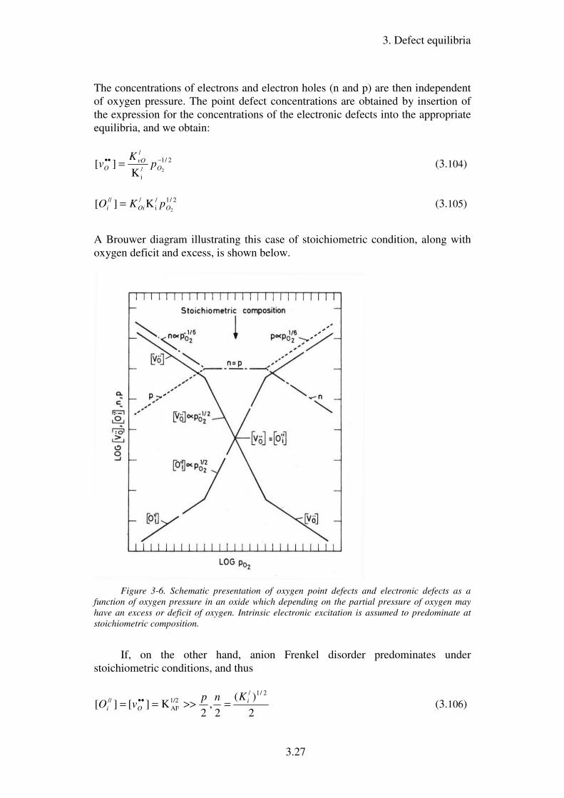
The concentrations of electrons and electron holes (n and p) are then independent
of oxygen pressure. The point defect concentrations are obtained by insertion of
the expression for the concentrations of the electronic defects into the appropriate
equilibria, and we obtain:
2/1
/
i
/
2K][ −•• = O
vO
O pK
v (3.104)
2/1/
i
///
2K][ OOii pKO = (3.105)
A Brouwer diagram illustrating this case of stoichiometric condition, along with
oxygen deficit and excess, is shown below.
Figure 3-6. Schematic presentation of oxygen point defects and electronic defects as a
function of oxygen pressure in an oxide which depending on the partial pressure of oxygen may
have an excess or deficit of oxygen. Intrinsic electronic excitation is assumed to predominate at
stoichiometric composition.
If, on the other hand, anion Frenkel disorder predominates under
stoichiometric conditions, and thus
2
)(
2,
2K][][
2/1/1/2
AF
// i
Oi
KnpvO =>>== •• (3.106)

3. Defect equilibria
3.28
then ][ //
iO and ][ ••Ov are independent of the partial pressure of oxygen, while the
concentrations of electronic defects are given by
4/14/12/1/
2)(n −−= OAFvO pKK (3.107)
4/14/12/1/
2)(p OAFOi pKK
−= (3.108)
A Brouwer diagram illustrating this case of stoichiometric condition, along with
oxygen deficit and excess, is shown below.
Figure 3-7. Schematic presentation of the concentration of oxygen point defects and
electronic defects as a function of oxygen pressure. Oxygen defects are assumed to predominate at
stoichiometric composition.
From the diagrams we can conclude that at low oxygen activities the oxide
has oxygen deficiency and will be an electronic n-type conductor, because the
mobility of the electrons is always much higher than that of oxygen vacancies. At
high oxygen partial pressures the oxide will correspondingly have oxygen excess
and be a p-type electronic conductor. At intermediate oxygen activities it may be
be a mixed n- and p-type electronic conductor in the case of intrinsic electronic
disorder, while it may exhibit ionic or mixed ionic/electronic conduction in the
case of anion Frenkel disorder.
Similar diagrams and analyses may be made for many other combinations of
non-stoichiometric and stoichiometric defect situations of pure (undoped) oxides
and other ionic compounds.

3. Defect equilibria
3.29
Summary
Chemical reactions for defects can be formulated and treated using the
mass-action law. As for other chemical reactions, equilibrium constants can be
defined in terms of the activities of the defects and other species. Under the
normal constrictions we can approximate activities with concentrations of defects
and partial pressures of gases. The equilibrium constants can also be expressed in
terms of the standard Gibbs energy change of the reaction, which in turn is a
function of the standard entropy and enthalpy changes.
We have seen that the standard entropy change of the standard Gibbs energy
change contains only vibrational terms of the standard states provided that the
configurational terms are properly handled in expressing the equilibrium
conditions. This is often possible in defect idealised defect chemistry since we can
apply classical statistical thermodynamics. However, for non-classical defects
such as delocalised electrons and holes this approach is less meaningful, and the
entropy change may then be interpreted in a less straightforward manner. We have
introduced the use of a prime (as in K/) to denote equilibrium constants that are
not expressed according to statistical thermodynamics and where the entropy
change in the Gibbs energy change may have other than vibrational contributions.
The mass action expressions can be combined with the full or limited cases
of the electroneutrality condition to obtain exact or approximate (limiting case)
expressions for the concentration of defects. Such concentrations are typically a
function of the oxygen partial pressure and temperature. It is common to illustrate
defect structures for oxides by plotting log defect concentrations vs log 2Op
(Brouwer diagrams) or ln or log defect concentrations vs 1/T (van ‘t Hoff plots).
We have shown these principles and techniques through examples of intrinsic
ionic and electronic disorder, various types of nonstoichiometry and variable
ionisation of point defects.
We have restricted our treatment to simple cases and made simplifications
where possible. Assumption of small defect concentrations have allowed the
assumptions that the concentrations of normal lattice atoms and empty interstitials
sites are constant, with activities equal to unity. (Larger defect concentrations can
to a first approximation be taken into account by including mass and site balances
into the expressions used to solve the defect structure.)
Literature
Kröger, F.A. (1964) The Chemistry of Imperfect Crystals, North-Holland,
Amsterdam, and Wiley, New York.
Kröger, F.A., Stieltjes, F.H. and Vink, H.J. (1959), Philips Res. Rept. 14,
557.

3. Defect equilibria
3.30
Problems
1. Do the insertion of Stirling’s approximation and the derivation that leads
up to the relation between equilibrium constant and entropy and enthalpy
changes for the elemental reaction EE = vE + EE (Eqs. 3.3 and onwards).
2. Write the reaction for formation of Schottky defects in MO2 and find an
expression for the defect concentrations as a function of the equilibrium
constant and thermodynamic parameters and temperature. Note in
particular how the solution deviates from the one obtained for the oxide
MO treated in the text.
3. In the case of cation Frenkel defects in MO we assumed in the text that we
had one interstitial site per MO. Derive the expression for the defect
concentrations if the structure consists of fcc close-packed O ions, with M
ions on each octahedral hole, and with interstitial sites on all tetrahedral
holes (Hint: consult Chapter 1). Does it deviate from Eq. (3.38)?
4. For a defect situation in an oxide dominated by doubly charged oxygen
vacancies and electrons, sketch the van ’t Hoff plot (Log defect
concentration vs 1/T) and a double-logarithmic plot of defect
concentrations vs pO2 (Brouwer diagram).
5. Consider a metal oxide MO1-y dominated by singly and doubly charged
oxygen vacancies. Suggest a condition that expresses the changeover from
dominance of one to dominance of the other.
6. Consider a metal oxide M2-xO3 dominated by doubly and triply charged
metal vacancies. Suggest a condition that expresses the changeover from
dominance of the doubly charged to dominance of the triply charged.
7. Find a general expression for m in the [e/] ∝ pO2
m relationship for oxides
MOb with non-stoichiometry dominated by fully ionised metal interstitials.
(Hint: Find m as a function of b). Use this to find m in the case of M2O,
MO, M2O3, MO2, M2O5 and MO3.
8. Find a general expression for m (as a function of the valency z of the
cation) in the [h.] ∝ pO2
m relationship for binary oxides with non-
stoichiometry dominated by fully ionised metal vacancies. Use this to find
m in the case of M2O3.
9. Sketch a full Brouwer diagram (log defect concentrations vs log pO2) for
an oxide M2O3 dominated by fully ionised oxygen and metal vacancies at
under- and overstoichiometry, respectively. Assume that Schottky defects
predominate close to stoichiometric conditions. (The main goal in this and
following Problems is to obtain and illustrate the pO2-dependencies. Use
the rules we listed for such constructions of Brouwer diagrams.)
10. Sketch a full Brouwer diagram (log defect concentrations vs log pO2) for
an oxide MO2 dominated by fully ionised oxygen and metal vacancies at
under- and overstoichiometry, respectively. Assume that intrinsic
electronic equilibrium predominates close to stoichiometric conditions.
11. Sketch a full Brouwer diagram (log defect concentrations vs log pO2) for
an oxide ABO3 dominated by fully ionised oxygen and metal vacancies at
under- and overstoichiometry, respectively. Assume that Schottky defects

3. Defect equilibria
3.31
predominate close to stoichiometric conditions. You may assume that both
cations are trivalent, but discuss also the effect it would have if A was
divalent and B tetravalent.
12. Sketch a full Brouwer diagram (log defect concentrations vs log pO2) for
an oxide AB2O4 dominated by fully ionised metal interstitials and
vacancies at under- and overstoichiometry, respectively. Assume that
Frenkel defects predominate close to stoichiometric conditions. You may
assume that A is divalent and B trivalent.
13. In the text we considered an oxide MO2 that had oxygen deficiency by
both fully charged oxygen vacancies and doubly charged metal
interstitials. Figure 3-5 illustrating the case was drawn assuming that the
ratio between the concentrations of the two defects was 105 at 1 atm pO2.
Calculate the exact pO2 at which the concentrations are equal.
3. Defect equilibria
3.32
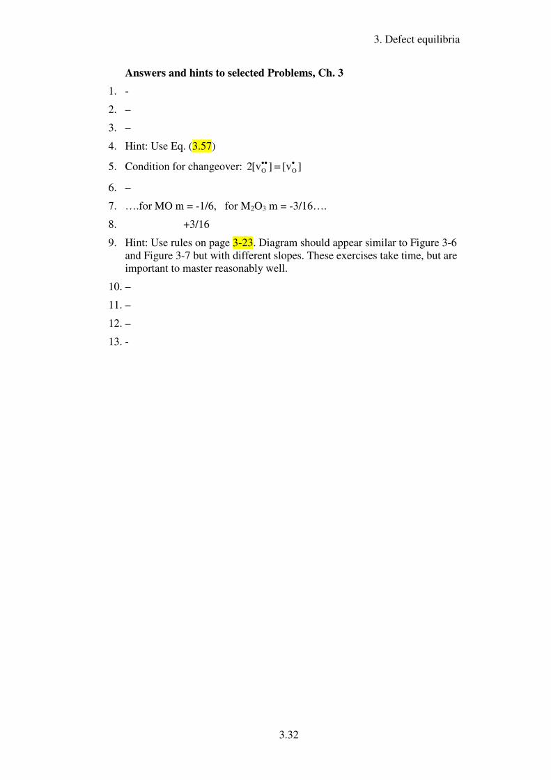
Answers and hints to selected Problems, Ch. 3
1. -
2. –
3. –
4. Hint: Use Eq. (3.57)
5. Condition for changeover: ][v][v2 OO
••• =
6. –
7. ….for MO m = -1/6, for M2O3 m = -3/16….
8. +3/16
9. Hint: Use rules on page 3-23. Diagram should appear similar to Figure 3-6
and Figure 3-7 but with different slopes. These exercises take time, but are
important to master reasonably well.
10. –
11. –
12. –
13. -