Accepted Manuscript

3-D local mesh refinement XFEM with variable-node hexahedronelements for extraction of stress intensity factors of straight and curvedplanar cracks

Zhen Wang, Tiantang Yu, Tinh Quoc Bui, Satoyuki Tanaka,Chuanzeng Zhang, Sohichi Hirose, Jose L. Curiel-Sosa

PII: S0045-7825(16)31306-8DOI: http://dx.doi.org/10.1016/j.cma.2016.10.011Reference: CMA 11172

To appear in: Comput. Methods Appl. Mech. Engrg.

Received date: 12 February 2016Revised date: 11 August 2016Accepted date: 4 October 2016

Please cite this article as: Z. Wang, T. Yu, T.Q. Bui, S. Tanaka, C. Zhang, S. Hirose, J.L.Curiel-Sosa, 3-D local mesh refinement XFEM with variable-node hexahedron elements forextraction of stress intensity factors of straight and curved planar cracks, Comput. MethodsAppl. Mech. Engrg. (2016), http://dx.doi.org/10.1016/j.cma.2016.10.011

This is a PDF file of an unedited manuscript that has been accepted for publication. As aservice to our customers we are providing this early version of the manuscript. The manuscriptwill undergo copyediting, typesetting, and review of the resulting proof before it is published inits final form. Please note that during the production process errors may be discovered whichcould affect the content, and all legal disclaimers that apply to the journal pertain.

1

Research Article:

3-D Local Mesh Refinement XFEM with Variable-Node Hexahedron

Elements for Extraction of Stress Intensity Factors of Straight and Curved

Planar Cracks

Zhen Wanga, Tiantang Yu a,*,#, Tinh Quoc Buib,c,*,†, Satoyuki Tanakad,

Chuanzeng Zhange, Sohichi Hirosec, Jose L. Curiel-Sosaf

aDepartment of Engineering Mechanics, Hohai University, Nanjing 211100, PR China. bInstitute for Research and Development, Duy Tan University, Da Nang City, Vietnam

cDepartment of Mechanical and Environmental Informatics, Tokyo Institute of Technology,

2-12-1-W8-22, Ookayama, Meguro-ku, Tokyo 152-8552, Japan. dGraduate School of Engineering, Hiroshima University, Higashi-Hiroshima 739-8527, Japan

eDepartment of Civil Engineering, University of Siegen, Germany fDepartment of Mechanical Engineering, The University of Sheffield, Sir Frederick Mappin

Building, Mappin Street, S1 3JD Sheffield, United Kingdom

*Corresponding authors: Duy Tan University, Da Nang City, Vietnam & Tokyo Institute of Technology, Japan

(T.Q. Bui); Hohai University, Nanjing, PR China (T.T. Yu)

Tel.: +81 (03) 57343587 (T.Q. Bui); Tel.: +86 (25) 52430342(T.T. Yu) #E-mail: tiantangyu@hhu.edu.cn (T.T. Yu) †E-mail: buiquoctinh@duytan.edu.vn; tinh.buiquoc@gmail.com (T. Q. Bui)

2

Abstract

A novel local mesh refinement approach for failure analysis of three-dimensional (3-D) linear

elastic solids is developed, considering both 3-D straight and curved planar cracks. The present local

mesh refinement formulation is in terms of the extended finite element methods and variable-node

hexahedron elements, driven by a posteriori error indicator. Our 3-D formulation using hexahedron

elements rigorously embraces a posteriori error estimation scheme, a structural coupling scale-meshes

strategy and an enrichment technique. Remeshing is only performed where it is needed, e.g., a vicinity

of crack, through an error estimator based on the recovery stress procedure. To treat the mismatching

problem induced by different scale-meshes in the domain, a structural coupling scheme employing

variable-node transition hexahedron elements based on the generic point interpolation with an arbitrary

number of nodes on each of their faces is presented. The 3-D finite element approximations of field

variables are enhanced by enrichments so that the mesh is fully independent of the crack geometry. The

displacement extrapolation method is taken for the evaluation of linear elastic fracture parameters (e.g.,

stress intensity factors - SIFs). To show the accuracy and performance of our 3-D proposed formulation,

six numerical examples of planar 3-D straight and curved shaped cracks with single and mixed-mode

fractures and different configurations are considered and analyzed. The SIFs computed by the

developed method are validated with respect to analytical solutions and the ones derived from the

conventional XFEM. Associated with an adaptive process, the present 3-D formulation allows the

analysts to gain a desirable accuracy with a few trials, which is suited for practices purpose.

Keywords: Fracture; XFEM; Error estimation; Adaptive; Variable-node element; 3D cracks;

Hexahedron element.

3

1. Introduction

Over the past few decades, studies on the numerical computations of fracture phenomena

of materials and structures has progressed significantly, which have had a tremendous impact

on engineering practice and design. Defects or cracks whose existence in structures is

unavoidable have a strong effect on the integrity and performance of engineering materials and

structures. Major cracks in structures must be fully considered to evaluate the residual strength

of cracked structures, which could essentially provide valuable information and knowledge to

the designers to mitigate the detrimental effects caused by cracks. Compared with the size of

structures, the geometry of crack is often small, and in order to represent the geometry of such a

crack, a fine mesh discretized for the cracked area is usually made. However, the computation

for that is obviously time-consuming, especially if the whole structure in 3-D discretized by a

fine mesh is taken. In some particular cases, the computational tasks even can not be conducted

successfully. The costs may be saved significantly if a coarser mesh is used for region without

cracks. As a result, a domain that comprises both fine and coarse meshes induces the

mismatching problem of different meshes, and an appropriate technique to couple the fine and

coarse meshes is hence needed.

Furthermore, another important problem that is often encountered in the vicinity of crack,

particularly near crack-tip, is the high gradients [1-3]. Modeling the high gradients using

mesh-based methods usually requires a fine mesh in the vicinity of crack. Therefore, accurate

solutions obtained by utilizing mesh-based methods (e.g., finite elements) are the results

derived from a model in which a fine mesh around the crack is used, while a coarser mesh is for

the rest of the body. The use of different meshes in such high gradient model also causes the

mismatching problems, and a structural coupling technique to link the meshes at different levels

is mandatory.

The numerical difficulty for the adoption of a non-uniform mesh is the treatment of

transition elements which have hanging nodes. Numerous special techniques have been

developed for treating the mismatching problems caused by different meshes such as the

Lagrange multipliers [4], projection method [5], penalty function parameters [6], mortar

method [7], Arlequin method [8]. Belytschko et al. [9] introduced a multiscale aggregating

discontinuity method to treat the discontinuity at macroscale level via the extended finite

4

element method (XFEM) [10]. The underlying characteristic of their model lies in the treatment

of material instabilities occurring in the micromodel, while an equivalent discontinuity is

injected into the macromodel. The method was then applied to the analysis of micro-macro

failure of composites [11, 12]. Plews and Duarte [13] developed a bridging multiple structural

scales aimed at resolving the challenging multiscale phenomena within the framework of the

generalized FEM with global-local enrichment functions. Loehnert and Belytschko [5] reported

an interesting work that combines the multiscale projection method and the XFEM for 2-D

macrocrack/microcrack at different length scales. With the aid of the projection method, the

resulting fine-scale stress fields are hence estimated onto the coarse-scale. There are several

other multiscale models available in literature, e.g., see Refs. [14-18], and the underlying idea

of those methods is to impose constraints at nodes on mismatching interfaces to connect

different scale meshes. Those methods however often require some modifications on the

system matrix whenever the constraints are imposed [19]. Kumar et al. [20, 21] proposed a

homogenized XFEM to simulate fatigue crack growth and a virtual node XFEM to represent

kinked cracks based on a non-uniform mesh. In order to ensure the continuity in the

displacement fields, six-node and five-node transition elements were developed, respectively.

Recently, the variable-node transition elements [19, 22], which have an arbitrary number

of nodes on the element sides and faces, are developed based on the generic point interpolation

for solving engineering problems. By using the variable-node elements, the mismatching

interfaces are converted into matching interfaces in a straightforward manner, thus the system

matrix does not need to be modified, an effective feature that does not valid in some of the

previous methods.

In light of XFEM developments, the authors have recently applied the XFEM to fracture

mechanics problems in multiphase homogeneous and nonhomogeneous functional smart

composite materials under static, dynamic and thermal coupled electromechanical loading

conditions, e.g., see Refs.[23-28]. Fatigue crack growth of interfacial cracks in bi-layered

functionally graded materials is also studied using the XFEM [29]. Recently, XFEM simulation

for cohesive crack growth in concrete structures with two new solution algorithms is presented

[30]. A stabilized discrete shear gap extended element is developed for cracked Mindlin plates

considering distorted mesh [31] and cracked functionally graded plates [32]. The XFEM for

5

hydraulic fracturing in rock mass is analyzed in [33]. More recently, the authors proposed an

enhanced XFEM using consecutive-interpolation procedure for accurately extracting stress

intensity factors as detailed in [34]. The authors have found that the standard XFEM is well

suited for modeling problems with non-smoothed solutions but to make the method more

flexible and effective in practical applications, we devote our motivation to the novel approach

that is reported in the present manuscript.

It is believed that the determination of accurate fracture parameters of straight or curved

cracks in 3-D configurations with mixed-mode loading remains a great challenge in the

computational fracture mechanics. Pathak et al. [35] proposed a simple and efficient XFEM

approach for 3-D cracks. A crack front is divided into a number of piecewise curve segments to

avoid an iterative solution. In crack front elements, the level set functions are approximated by

higher order shape functions which assure the accurate modeling of the crack front. Later, they

applied the method to model fatigue crack growth simulations of 3-D problems [36, 37].

Sharma et al. [38] employed XFEM to obtain the stress intensity factors of a semi-elliptical part

through thickness axial crack. Level set functions are approximated using higher order shape

functions in the crack front elements to ensure the accurate modeling of the crack. This paper

particularly focuses on the development of an effective and accurate local mesh refinement

XFEM (Lm-XFEM) using hexahedron elements to accurately estimate linear elastic fracture

parameters of both planar 3-D straight and curved cracks. The proposed approach runs with an

engine embracing three components of tackling different tasks, an adaptation algorithm for

local mesh refinement, an enrichment scheme for capturing the cracks, and a coupling method

for treating mismatching meshes in the model.

In the present Lm-XFEM formulation, an adaptive algorithm whose role is to refine the

elements is required. The elements to be refined have been detected by a posteriori error

estimation algorithm. The adaptive procedure using a posteriori error estimation in terms of the

XFEM is adopted from the work done by Prange et al. [3]. The Zienkiewicz and Zhu error

estimator [39] is used and that is based on a stress smoothing technique. The enhanced

smoothed stresses incorporating the discontinuities and singularities induced by cracks are

recovered, by which the error estimation for arbitrary distributed cracks can be made. It is noted

that every stress component is recovered separately and the nodal enhanced smoothed stresses

6

are recovered with a least square fit. An error indicator applied to subsequently refined meshes

is gained with a relative error, and every element with a relative error exceeds a given specified

value of tolerance error is then refined with a set of subdivision elements. For further

information, interested readers can refer to [2, 3, 18].

The Lm-XFEM utilizing the variable-node hexahedron elements [19, 22] with an arbitrary

number of nodes on each of their faces is to couple the meshes at different levels; while the

enrichment scheme [10, 40] for describing the discontinuities induced by the crack surfaces and

the singularities because of crack front is taken. Notice that the variable-node hexahedron

elements [19, 22] are further extended to carry cracks in this work. In fact, unlike the problems

with smoothed solutions, the problems under investigation involving cracks (or non-smoothed

solutions type) require not only a regular variable-node element, but also a variable-node

element that can carry crack. As can be seen in the subsequent sections the variable-node

hexahedron elements can be cut by a crack or contain a crack-tip, which do exist in the present

model. Therefore, such cut and crack-tip variable-node hexahedron transition elements must be

developed as well to fully assure the compatibility of the configuration, the convergence of the

solutions or avoid the undesirable behaviors.

The Lm-XFEM enables one to utilize a refined mesh only in the vicinity of the crack

where it is required, and the matching interfaces between different meshes are directly obtained.

Therefore, small crack sizes can be considered in the analysis of the whole large structures and

the accuracy of the solutions around the cracks can be significantly improved with a low cost.

More importantly the accuracy of the results is controllable.

It is also worth noting that the traditional fixed-node element is one special case for the

variable-node elements, hence the variable-node hexahedron elements can be implemented

within an existing 3-D XFEM computer code with little modification and effort. The

Lm-XFEM associated with an adaptive process allows the users to achieve desired accuracies

with some trials. Another important point is that each node of the variable-node hexahedron

element has its own degree of freedom and a symmetric system matrix is constructed in the

same way as the standard FEM [19].

It is known that the most important characterizing fracture parameters to represent the

strength of the singular fields at the crack tips in 2-D and crack front in 3-D are the stress

7

intensity factors (SIFs). Several well-known methods have been proposed to determine the SIFs,

and in this paper the displacement extrapolation method near the crack tip [41] is adopted for

our 3-D straight and curved cracks. We will again discuss this issue a bit more detail in the

subsequent sections. Basically, the displacement extrapolation method can be used for direct

evaluation of the SIFs according to the relative crack surface displacements.

It is very important to mention here that our aim is to develop a novel effective local mesh

refinement in terms of XFEM for the simulation of cracks in 3-D, and thus this paper does not

devote to a micro-macro multiscale failure analysis. A misleading/misunderstanding of

multiscale failure of solids in terms of homogenization frame however should be avoided.

The body of paper is structured as follows. In Section 2, the 3-D Lm-XFEM formulation is

presented in which the variable-node hexahedron elements to link the different scale elements,

a posteriori recovery-based error estimator for the adaptive purpose, numerical integration,

enriched displacement approximations, etc. are detailed. Computation of 3-D stress intensity

factors (SIFs) using the displacement extrapolation method is briefly described in Section 3.

Numerical examples are analyzed and discussed in Section 4, and some conclusions and

outlook drawn from the study are given in Section 5.

2. Formulation of three-dimensional local mesh refinement XFEM

2.1 Enriched finite element approximation

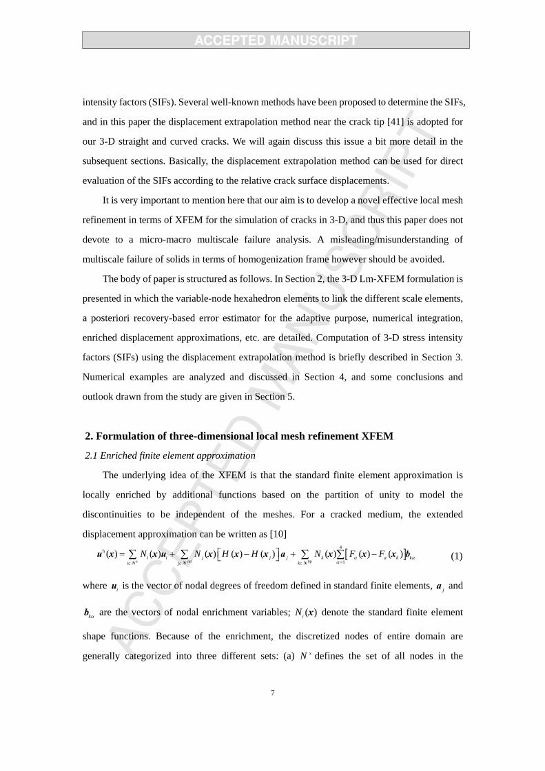
The underlying idea of the XFEM is that the standard finite element approximation is

locally enriched by additional functions based on the partition of unity to model the

discontinuities to be independent of the meshes. For a cracked medium, the extended

displacement approximation can be written as [10]

[ ]cut tip

4h

1( ) ( ) ( ) ( ) ( ) ( ) ( ) ( )

si i j j j k k k

i j k

N N H H N F Fα α αα =∈ ∈ ∈

⎡ ⎤= + − + −⎣ ⎦∑ ∑ ∑ ∑N N N

u x x u x x x a x x x b (1)

where iu is the vector of nodal degrees of freedom defined in standard finite elements, ja and

kαb are the vectors of nodal enrichment variables; ( )iN x denote the standard finite element

shape functions. Because of the enrichment, the discretized nodes of entire domain are

generally categorized into three different sets: (a) sN defines the set of all nodes in the

8

discretization; (b) cutN is the set of nodes whose basis function support is entirely split by the

crack and are enriched with a discontinuous Heaviside function ( )H x . The function takes on

the value +1 above the crack and -1 below the crack; and (c) tipN is the last one that defines the

set of nodes enriched with the asymptotic crack-tip enrichment functions ( )Fα x ( 1, ,4)α = .

The set tipN represents the set of nodes whose basis function support is partly split by the crack.

To model the crack front and to represent the crack-tip fields in 3-D isotropic elasticity

computation, the 2-D crack-tip branch enrichment functions ( )Fα x are used in elements which

contain the crack front, and are given by

( ) , 1, , 4 sin cos sin sin cos sin2 2 2 2

F r r r rαθ θ θ θα θ θ⎡ ⎤= =⎡ ⎤⎣ ⎦ ⎢ ⎥⎣ ⎦

x (2)

where r and θ are the crack-tip polar co-ordinates.

In XFEM, crack surfaces are often described by using the level sets. Two signed distance

functions are defined to describe a 3-D crack. Two iso-zero level sets can define the crack

location, and the enrichment type of each node can be determined according to the value of

nodal level set function [42]. Sukumar et al. [40] discussed the computational geometry issues

associated with the representation of the crack and the enrichment of the finite element

approximation in detail.

Remark #1: It is important to point out here that the 2-D crack-tip branch enrichments in

Eq. (2) are also valid for 3-D crack problems. Preceding studies [40, 42] already indicate that

the asymptotic fields are two-dimensional in nature in the neighborhood of the crack front in

3-D problems. Also notice that only the first term of the enrichment functions is discontinuous

while others are added to enhance the accuracy in elastic fracture mechanics problems. The 2-D

branch functions in Eq. (2) span the near-tip asymptotic solutions for an elastic crack in two

dimensions, and more importantly, Sukumar et al. [40] and Moës et al. [42] have found that

such 2-D basis to be quite adequate accuracy for 3-D crack problems.

Remark #2: Blending elements do exist in the displacement approximation shown in Eq.

(1). Blending elements in the XFEM may reduce the overall convergence rate as stated in [43].

Some approaches have been proposed to treat the blending elements, and these approaches may

be divided into four categories: corrected or weighted XFEM [44, 45], suppressing blending

9

elements by coupling enriched and standard regions [43, 46], hierarchical shape functions in

blending elements [47], and assumed strain blending elements [48]. In this study, the blending

element issue is not considered, but it would be a potential work for our future study.

2.2 Linkage meshes technique using variable-node transition elements

One layer of variable-node transition elements exists between two different scale elements

as schematically represented in yellow in Fig. 1 for hexahedron elements. The variable-node

elements [19], which have an arbitrary number of nodes on the element faces, with special

bases that have slope discontinuities in 3-D domains, and the elements retain the linear

interpolation between any two neighboring nodes. As stated by Sohn et al. [19] or Lim et al. [22]

that the variable-node elements can provide a flexibility to resolve non-mismatching mesh

problems like the mesh connection and adaptive mesh refinement. It hence motivates us to

adopt the variable-node elements to solve the mismatching problems of different scale meshes

in the present formulation.

(a)

(b)

Fig. 1 Hexahedral meshes discretization of a straight edge crack in a 3-D solid containing two

different scale hexahedron elements (a). Schematically showing one layer of variable-node

transition hexahedron elements connected two different meshes as marked in yellow and its

front view (b). The blue line represents the crack.

Let us consider the approximate displacements h ( )u ξ for ( )u ξ by the point interpolation,

10

with pN based-polynomials, h ( )u ξ can then be expressed as follows:

( ) ( )h

1( )

pNT

i ii=

= =∑u ξ N ξ u a p ξ (3)

where pN is the number of sampling points in the point interpolation;

0 00 00 0

i

i i

i

NN

N

⎡ ⎤⎢ ⎥= ⎢ ⎥⎢ ⎥⎣ ⎦

N (4)

is the shape function matrix, in which iN is the shape function that is associated with node i;

[ ]T

i i i iu v w=u is the nodal variable vector; Ta is the 3 × pN matrix of the unknown

coefficients while ( )p ξ is the pN × 1 column vector of the polynomial basis.

For the eight-node hexahedron element, the polynomial basis can be given by

( ) [ ]T1 ξ η ζ ξη ηζ ξζ ξηζ=p ξ (5)

where ξ , η and ζ are the local coordinates in the isoparametric element.

The point interpolation follows that is then expressed as

( ) ( )h T T -1( ) = =u ξ a p ξ U q p ξ (6)

with

[ ]1 8...=q p p (7)

[ ]T1 8...=U u u (8)

From Eqs. (3) to (8), the shape functions of the eight-node hexahedron element are

obtained and are written in general form as

( ) ( )( ) ( )1 1 1 1+8i i i iN ξξ ηη ζζ= + +ξ (9)

By adding some extra special basis to meet the point interpolation characteristics,

variable-node elements can then be generated. Basically, the choice for the extra special basis

often depends on the interpolation type that is required on the element-surfaces. A linear

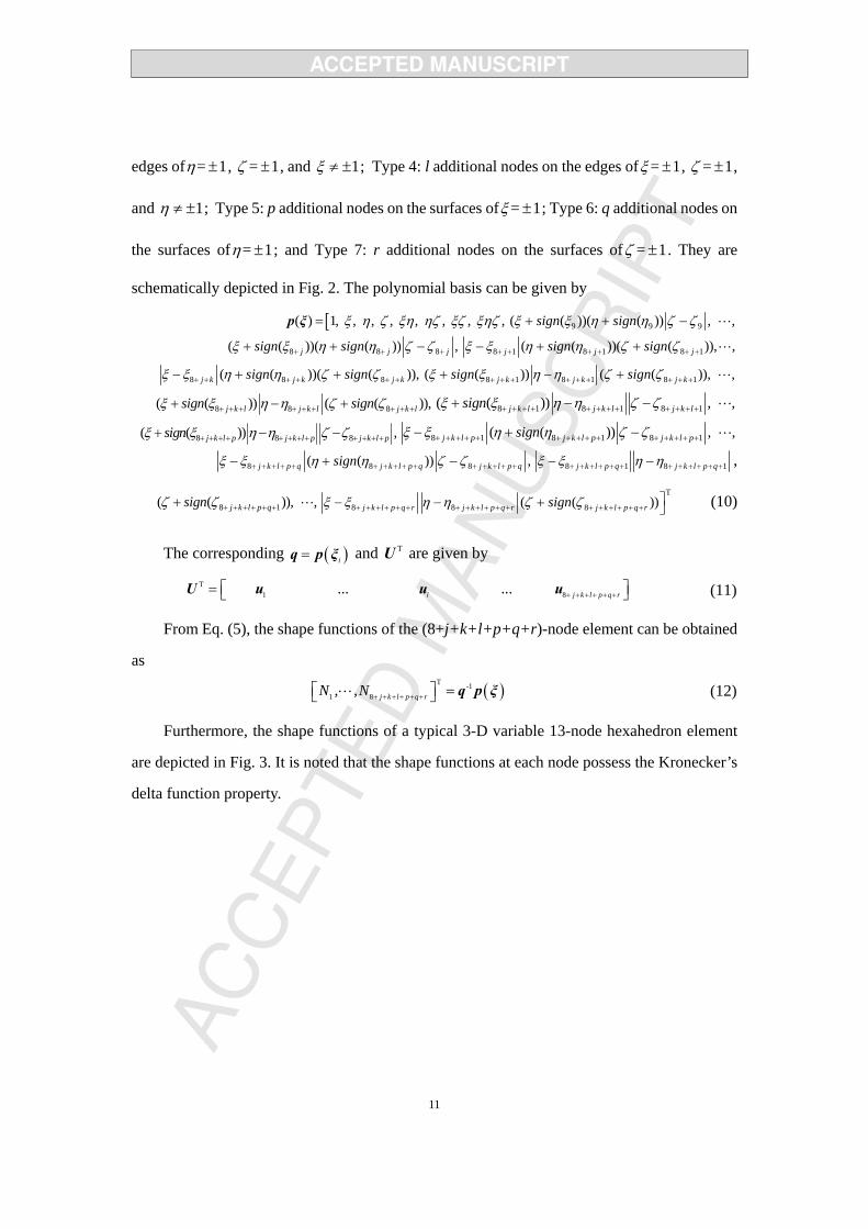
variable-node hexahedron element, that is called as a (8+j+k+l+p+q+r)-node element, all

nodes can be divided into 7 types as follow: Type 1: 8 corner nodes of the hexahedron element;

Type 2: j nodes on the edges of = 1ξ ± ， = 1η ± , and 1ζ ≠ ± ; Type 3: k additional nodes on the

11

edges of = 1η ± , = 1ζ ± , and 1ξ ≠ ± ; Type 4: l additional nodes on the edges of = 1ξ ± , = 1ζ ± ,

and 1η ≠ ± ; Type 5: p additional nodes on the surfaces of = 1ξ ± ; Type 6: q additional nodes on

the surfaces of = 1η ± ; and Type 7: r additional nodes on the surfaces of = 1ζ ± . They are

schematically depicted in Fig. 2. The polynomial basis can be given by

[( ) 1, , , , , , , ,ξ η ζ ξη ηζ ξζ ξηζ=p ξ 9 9 9( ( ))( ( )) , ,sign signξ ξ η η ζ ζ+ + −

8 8 8( ( ))( ( )) ,j j jsign signξ ξ η η ζ ζ+ + ++ + − 8 1 8 1 8 1( ( ))( ( )), ,j j jsign signξ ξ η η ζ ζ+ + + + + +− + +

8 8 8( ( ))( ( )),j k j k j ksign signξ ξ η η ζ ζ+ + + + + +− + + 8 1 8 1 8 1( ( )) ( ( )), ,j k j k j ksign signξ ξ η η ζ ζ+ + + + + + + + ++ − +

8 8 8( ( )) ( ( )),j k l j k l j k lsign signξ ξ η η ζ ζ+ + + + + + + + ++ − + 8 1 8 1 8 1( ( )) , ,j k l j k l j k lsignξ ξ η η ζ ζ+ + + + + + + + + + + ++ − −

8 8 8( ( )) ,j k l p j k l p j k l psignξ ξ η η ζ ζ+ + + + + + + + + + + ++ − − 8 1 8 1 8 1( ( )) , ,j k l p j k l p j k l psignξ ξ η η ζ ζ+ + + + + + + + + + + + + + +− + −

8 8 8( ( )) ,j k l p q j k l p q j k l p qsignξ ξ η η ζ ζ+ + + + + + + + + + + + + + +− + − 8 1 8 1j k l p q j k l p qξ ξ η η+ + + + + + + + + + + +− − ,

8 1( ( )), ,j k l p qsignζ ζ + + + + + ++T

8 8 8( ( ))j k l p q r j k l p q r j k l p q rsignξ ξ η η ζ ζ+ + + + + + + + + + + + + + + + + +⎤− − + ⎦ (10)

The corresponding ( )i=q p ξ and TU are given by

T1 8i j k l p q r... ... + + + + + +⎡ ⎤= ⎣ ⎦U u u u (11)

From Eq. (5), the shape functions of the (8+j+k+l+p+q+r)-node element can be obtained

as

( )T -11 8 j k l p q rN , ,N + + + + + +⎡ ⎤ =⎣ ⎦ q p ξ (12)

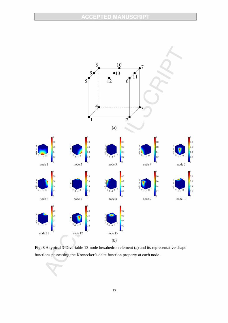
Furthermore, the shape functions of a typical 3-D variable 13-node hexahedron element

are depicted in Fig. 3. It is noted that the shape functions at each node possess the Kronecker’s

delta function property.

12

Fig. 2 Schematic notation of a (8+j+k+l+p+q+r)-node element and the definition of its

division into seven types of different grouped nodes.

13

(a)

(b)

Fig. 3 A typical 3-D variable 13-node hexahedron element (a) and its representative shape

functions possessing the Kronecker’s delta function property at each node.

14

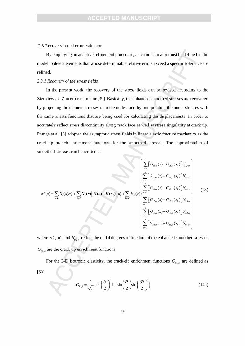
2.3 Recovery based error estimator

By employing an adaptive refinement procedure, an error estimator must be defined in the

model to detect elements that whose determinable relative errors exceed a specific tolerance are

refined.

2.3.1 Recovery of the stress fields

In the present work, the recovery of the stress fields can be revised according to the

Zienkiewicz–Zhu error estimator [39]. Basically, the enhanced smoothed stresses are recovered

by projecting the element stresses onto the nodes, and by interpolating the nodal stresses with

the same ansatz functions that are being used for calculating the displacements. In order to

accurately reflect stress discontinuity along crack face as well as stress singularity at crack tip,

Prange et al. [3] adopted the asymptotic stress fields in linear elastic fracture mechanics as the

crack-tip branch enrichment functions for the smoothed stresses. The approximation of

smoothed stresses can be written as

3

11, 11, 11,1

3

22, 22, 22,1

3

33, 33, 33,1

3

12, 12, 12,1

13, 13,

( ) ( )

( ) ( )

( ) ( )( ) ( ) ( ) ( ) ( ) ( )

( ) ( )

( )

k k

k k

k ks

i i j j j ki j

k k

G x G x b

G x G x b

G x G x bx N x N x H x H x a N x

G x G x b

G x G

α α αα

α α αα

α α αα

α α αα

α

σ σ

∗

=

∗

=

∗

=∗ ∗

∈ ∈ ∗

=

⎡ ⎤−⎣ ⎦

⎡ ⎤−⎣ ⎦

⎡ ⎤−⎣ ⎦⎡ ⎤= + − +⎣ ⎦

⎡ ⎤−⎣ ⎦

−

∑

∑

∑∑ ∑

∑I J

3

13,1

3

23, 23, 23,1

( )

( ) ( )

k

k k

k k

x b

G x G x b

α αα

α α αα

∈

∗

=

∗

=

⎧ ⎫⎪ ⎪⎪ ⎪⎪ ⎪⎪ ⎪⎪ ⎪⎪ ⎪⎪ ⎪⎪ ⎪⎨ ⎬⎪ ⎪⎪ ⎪⎪ ⎪⎪ ⎪⎡ ⎤⎣ ⎦⎪ ⎪⎪ ⎪⎪ ⎪⎡ ⎤−⎣ ⎦⎪ ⎪⎩ ⎭

∑

∑

∑

K

(13)

where iσ∗ , ja∗ and ,pq kb∗ reflect the nodal degrees of freedom of the enhanced smoothed stresses.

pq,G α are the crack tip enrichment functions.

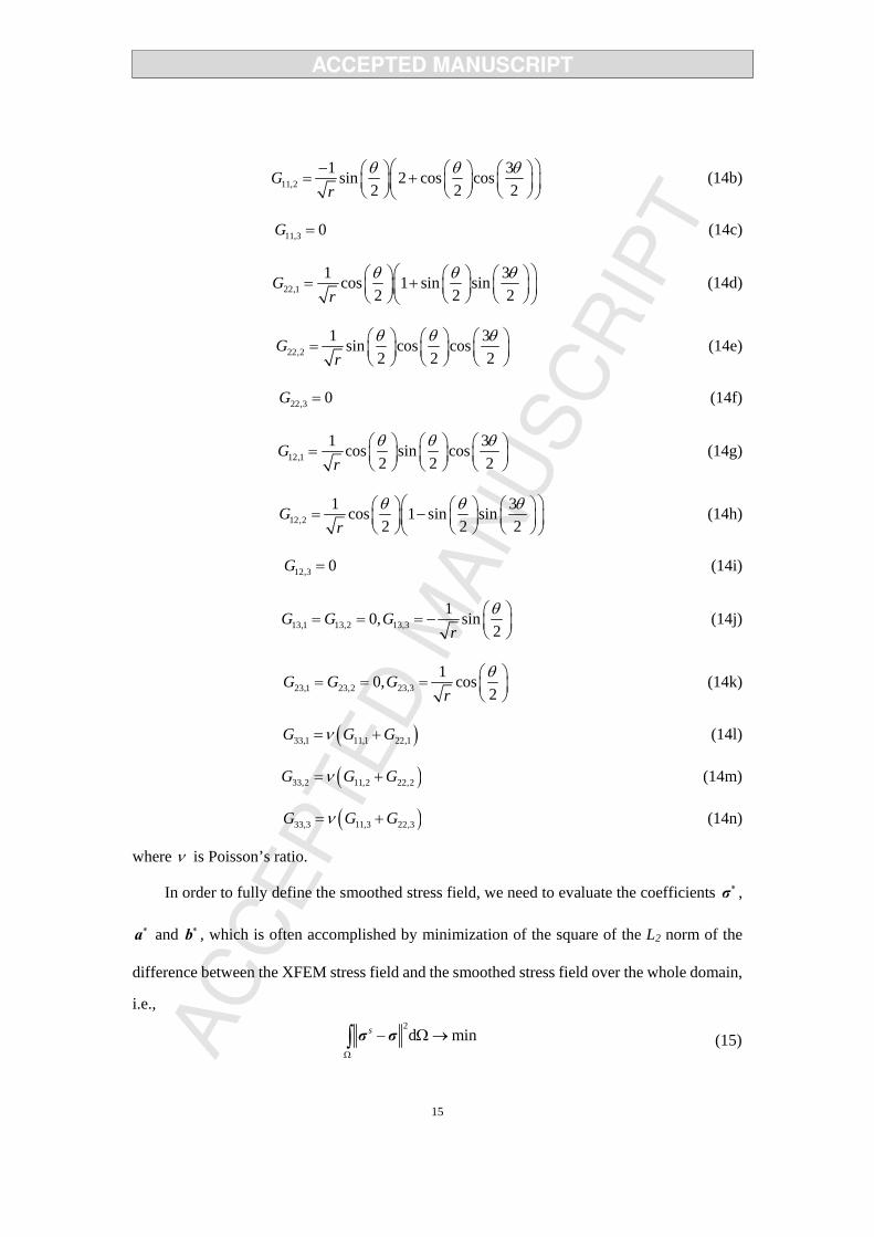
For the 3-D isotropic elasticity, the crack-tip enrichment functions pq,G α are defined as

[53]

11,11 3cos 1 sin sin

2 2 2G

rθ θ θ⎛ ⎞⎛ ⎞ ⎛ ⎞ ⎛ ⎞= −⎜ ⎟ ⎜ ⎟ ⎜ ⎟⎜ ⎟⎝ ⎠ ⎝ ⎠ ⎝ ⎠⎝ ⎠

(14a)

15

11,21 3sin 2 cos cos

2 2 2G

rθ θ θ− ⎛ ⎞⎛ ⎞ ⎛ ⎞ ⎛ ⎞= +⎜ ⎟ ⎜ ⎟ ⎜ ⎟⎜ ⎟⎝ ⎠ ⎝ ⎠ ⎝ ⎠⎝ ⎠

(14b)

11,3 0G = (14c)

22,11 3cos 1 sin sin

2 2 2G

rθ θ θ⎛ ⎞⎛ ⎞ ⎛ ⎞ ⎛ ⎞= +⎜ ⎟ ⎜ ⎟ ⎜ ⎟⎜ ⎟⎝ ⎠ ⎝ ⎠ ⎝ ⎠⎝ ⎠

(14d)

22,21 3sin cos cos

2 2 2G

rθ θ θ⎛ ⎞ ⎛ ⎞ ⎛ ⎞= ⎜ ⎟ ⎜ ⎟ ⎜ ⎟⎝ ⎠ ⎝ ⎠ ⎝ ⎠

(14e)

22,3 0G = (14f)

12,11 3cos sin cos

2 2 2G

rθ θ θ⎛ ⎞ ⎛ ⎞ ⎛ ⎞= ⎜ ⎟ ⎜ ⎟ ⎜ ⎟⎝ ⎠ ⎝ ⎠ ⎝ ⎠

(14g)

12,21 3cos 1 sin sin

2 2 2G

rθ θ θ⎛ ⎞⎛ ⎞ ⎛ ⎞ ⎛ ⎞= −⎜ ⎟ ⎜ ⎟ ⎜ ⎟⎜ ⎟⎝ ⎠ ⎝ ⎠ ⎝ ⎠⎝ ⎠

(14h)

12,3 0G = (14i)

13,1 13,2 13,310, sin

2G G G

rθ⎛ ⎞= = = − ⎜ ⎟⎝ ⎠

(14j)

23,1 23,2 23,310, cos

2G G G

rθ⎛ ⎞= = = ⎜ ⎟⎝ ⎠

(14k)

( )33,1 11,1 22,1G G Gν= + (14l)

( )33,2 11,2 22,2G G Gν= + (14m)

( )33,3 11,3 22,3G G Gν= + (14n)

where ν is Poisson’s ratio.

In order to fully define the smoothed stress field, we need to evaluate the coefficients ∗σ ,

∗a and ∗b , which is often accomplished by minimization of the square of the L2 norm of the

difference between the XFEM stress field and the smoothed stress field over the whole domain,

i.e., 2d mins

Ω

− Ω→∫ σ σ (15)

16

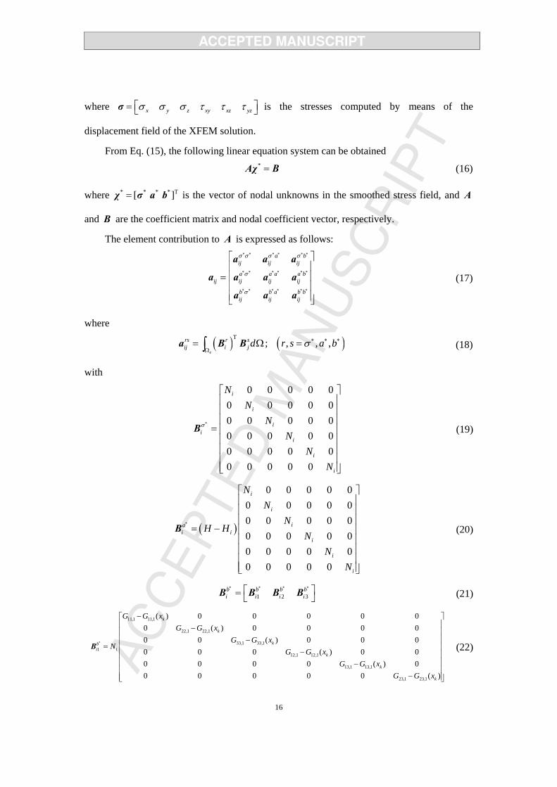
where x y z xy xz yzσ σ σ τ τ τ⎡ ⎤= ⎣ ⎦σ is the stresses computed by means of the

displacement field of the XFEM solution.

From Eq. (15), the following linear equation system can be obtained * =Aχ B (16)

where * * * * T[ ]=χ σ a b is the vector of nodal unknowns in the smoothed stress field, and A

and B are the coefficient matrix and nodal coefficient vector, respectively.

The element contribution to A is expressed as follows: a b

ij ij ij

a a a a bij ij ij ij

b b a b bij ij ij

σ σ σ σ

σ

σ

∗ ∗ ∗ ∗ ∗ ∗

∗ ∗ ∗ ∗ ∗ ∗

∗ ∗ ∗ ∗ ∗ ∗

⎡ ⎤⎢ ⎥⎢ ⎥=⎢ ⎥⎢ ⎥⎣ ⎦

a a a

a a a a

a a a

(17)

where

( ) ( ); , , ,e

rs r sij i j d r s a bσ

Τ ∗ ∗ ∗

Ω= Ω =∫a B B (18)

with

0 0 0 0 00 0 0 0 00 0 0 0 00 0 0 0 00 0 0 0 00 0 0 0 0

i

i

ii

i

i

i

NN

NN

NN

σ∗

⎡ ⎤⎢ ⎥⎢ ⎥⎢ ⎥

= ⎢ ⎥⎢ ⎥⎢ ⎥⎢ ⎥⎢ ⎥⎣ ⎦

Β (19)

( )

0 0 0 0 00 0 0 0 00 0 0 0 00 0 0 0 00 0 0 0 00 0 0 0 0

i

i

iai i

i

i

i

NN

NH H

NN

N

∗

⎡ ⎤⎢ ⎥⎢ ⎥⎢ ⎥

= − ⎢ ⎥⎢ ⎥⎢ ⎥⎢ ⎥⎢ ⎥⎣ ⎦

B (20)

1 2 3b b b bi i i i

∗ ∗ ∗ ∗⎡ ⎤= ⎣ ⎦B B B B (21)

11,1 11,1

22,1 22,1

33,1 33,11

12,1 12,1

13,1 13,1

23,1 23,1

( ) 0 0 0 0 00 ( ) 0 0 0 00 0 ( ) 0 0 00 0 0 ( ) 0 00 0 0 0 ( ) 00 0 0 0 0 ( )

k

k

kbi i

k

k

k

G G xG G x

G G xN

G G xG G x

G G x

∗

−⎡ ⎤⎢ ⎥−⎢ ⎥⎢ ⎥−

= ⎢ ⎥−⎢ ⎥⎢ ⎥−⎢ ⎥

−⎢ ⎥⎣ ⎦

B

(22)

17

11,2 11,2

22,2 22,2

33,2 33,22

12,2 12,2

13,2 13,2

23,2 23,2

( ) 0 0 0 0 00 ( ) 0 0 0 00 0 ( ) 0 0 00 0 0 ( ) 0 00 0 0 0 ( ) 00 0 0 0 0 ( )

k

k

kbi i

k

k

k

G G xG G x

G G xN

G G xG G x

G G x

∗

−⎡ ⎤⎢ ⎥−⎢ ⎥⎢ ⎥−

= ⎢ ⎥−⎢ ⎥⎢ ⎥−⎢ ⎥

−⎢ ⎥⎣ ⎦

B

(23)

11,3 11,3

22,3 22,3

33,3 33,33

12,3 12,3

13,3 13,3

23,3 23,3

( ) 0 0 0 0 00 ( ) 0 0 0 00 0 ( ) 0 0 00 0 0 ( ) 0 00 0 0 0 ( ) 00 0 0 0 0 ( )

k

k

kbi i

k

k

k

G G xG G x

G G xN

G G xG G x

G G x

∗

−⎡ ⎤⎢ ⎥−⎢ ⎥⎢ ⎥−

= ⎢ ⎥−⎢ ⎥⎢ ⎥−⎢ ⎥

−⎢ ⎥⎣ ⎦

B

(24)

and the element contribution to B is as follows a b

i i i iσ ∗ ∗ ∗⎡ ⎤= ⎣ ⎦b b b b (25)

ei i dσ σ σ

∗ ∗

Ω= Ω∫b B (26)

e

a ai i dσ∗ ∗

Ω= Ω∫b B (27)

e

b bi i dσ∗ ∗

Ω= Ω∫b B (28)

2.3.2 Error estimator

As the error estimator is based on a stress smoothing method, the nodal enhanced stresses

are hence recovered with a least square fit. The L2 norm error of stresses for element i is

computed at the element level by the following equation [3]

( ) ( ) ( )1 de

Ts s

e

err iΩ

= − − ΩΩ ∫ σ σ σ σ (29)

with eΩ being the area of the element. The maximum L2 norm stress of the elements is maxerr ,

then the relative discretization error for element i is estimated as

( ) ( )max

err100%

erri

iη = × (30)

This factor is known as an error indicator applicable to subsequently refined meshes, and every

element (called parent elements) with a relative discretization error greater than a specified

permitted value is refined with a set of sub-elements (called children elements). In this 3-D

work, a set of 3 3 3× × sub-division elements or children elements is used throughout the study

18

unless stated otherwise. One must be noted that this adaptive refinement procedure naturally

leads to incompatible hanging nodes between parents and children elements. However, the

incompatible feature of the meshes is then merged by the aid of the variable-node transition

elements [19, 22].

The L2 norm error of the stresses for the whole domain is then calculated by

( ) ( )Total de

Ts serrΩ

= − − Ω∫ σ σ σ σ (31)

2.4 Numerical integrations

In the present Lm-XFEM, there exist different types of elements mainly induced by cracks

and different scale meshes. The numerical integration used for those elements is crucial and

important to the success of the approach. The influence of the numerical integration on the

performance and the accuracy of the XFEM in general or the present Lm-XFEM in particular is

not trivial. Previous efforts have devoted to the development of effective and accurate methods

for the numerical integration in the context of the XFEM. Relevant references are not given

here due to the sake of brevity of the manuscript, but interested readers may find them in the

literature effortlessly.

To ensure the strain field to be adequately integrated, the following integration schemes

are utilized in the present formulation.

(1) Eight-node hexahedron elements: For the eight-node hexahedron elements, the

conventional second-order Gaussian quadrature scheme is employed for treating elements that

do not contain any enriched nodes. For the elements that include enriched nodes (but are not cut

by the crack), high-order Gaussian quadrature rule is handled to improve the accuracy of the

results. However, it needs a special treatment of the numerical integration for the elements that

are cut by a crack or contain a crack-front, called “cut element” and “crack-front element”,

respectively. The treatment can be fulfilled by partitioning the cut or split elements and

crack-front elements into sub-tetrahedrons, as schematically shown in Fig.4, whose boundaries

align with the crack geometry, e.g., see also Refs.[10, 40] for more information. In the

sub-tetrahedrons, high-order Gaussian quadrature rules are often taken to ensure and improve

the accuracy of the results. Nonetheless, the use of the Gaussian points for all the computations

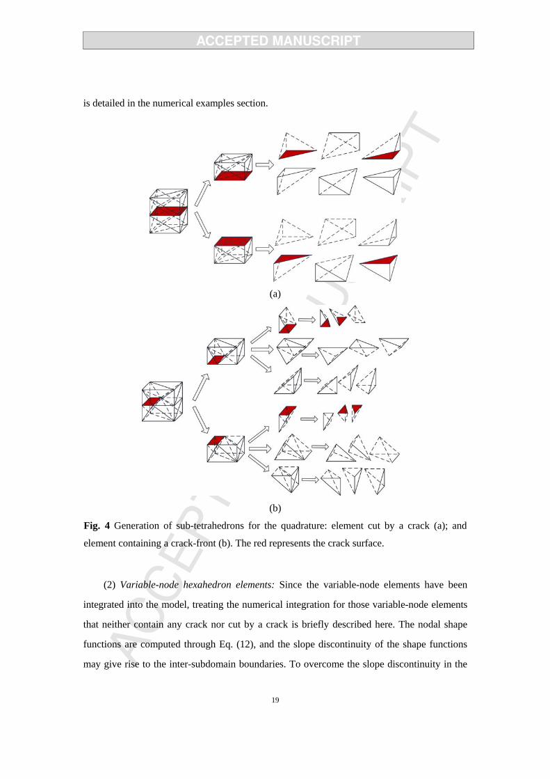
19

is detailed in the numerical examples section.

(a)

(b)

Fig. 4 Generation of sub-tetrahedrons for the quadrature: element cut by a crack (a); and

element containing a crack-front (b). The red represents the crack surface.

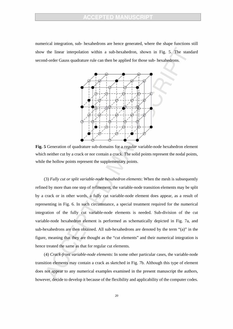
(2) Variable-node hexahedron elements: Since the variable-node elements have been

integrated into the model, treating the numerical integration for those variable-node elements

that neither contain any crack nor cut by a crack is briefly described here. The nodal shape

functions are computed through Eq. (12), and the slope discontinuity of the shape functions

may give rise to the inter-subdomain boundaries. To overcome the slope discontinuity in the

20

numerical integration, sub- hexahedrons are hence generated, where the shape functions still

show the linear interpolation within a sub-hexahedron, shown in Fig. 5. The standard

second-order Gauss quadrature rule can then be applied for those sub- hexahedrons.

Fig. 5 Generation of quadrature sub-domains for a regular variable-node hexahedron element

which neither cut by a crack or nor contain a crack. The solid points represent the nodal points,

while the hollow points represent the supplementary points.

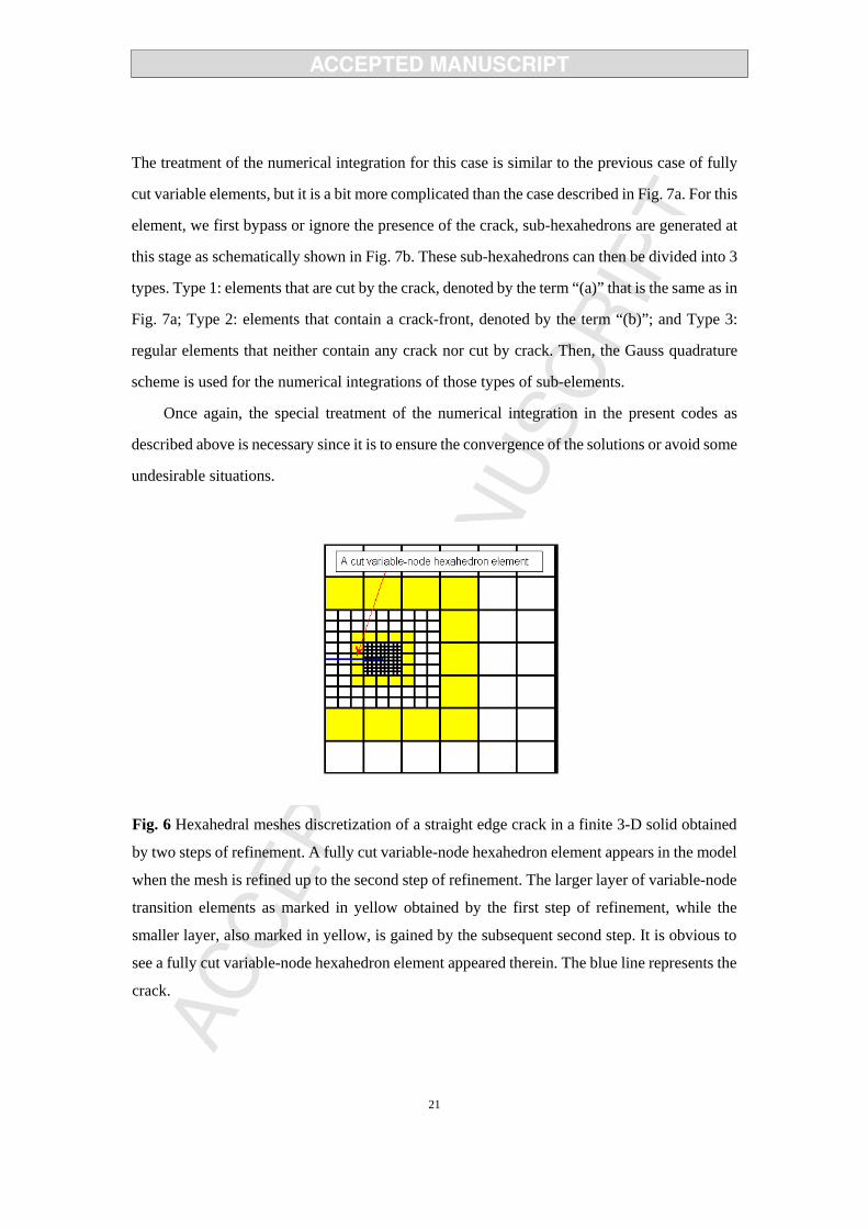
(3) Fully cut or split variable-node hexahedron elements: When the mesh is subsequently

refined by more than one step of refinement, the variable-node transition elements may be split

by a crack or in other words, a fully cut variable-node element does appear, as a result of

representing in Fig. 6. In such circumstance, a special treatment required for the numerical

integration of the fully cut variable-node elements is needed. Sub-division of the cut

variable-node hexahedron element is performed as schematically depicted in Fig. 7a, and

sub-hexahedrons are then obtained. All sub-hexahedrons are denoted by the term “(a)” in the

figure, meaning that they are thought as the “cut elements” and their numerical integration is

hence treated the same as that for regular cut elements.

(4) Crack-front variable-node elements: In some other particular cases, the variable-node

transition elements may contain a crack as sketched in Fig. 7b. Although this type of element

does not appear to any numerical examples examined in the present manuscript the authors,

however, decide to develop it because of the flexibility and applicability of the computer codes.

21

The treatment of the numerical integration for this case is similar to the previous case of fully

cut variable elements, but it is a bit more complicated than the case described in Fig. 7a. For this

element, we first bypass or ignore the presence of the crack, sub-hexahedrons are generated at

this stage as schematically shown in Fig. 7b. These sub-hexahedrons can then be divided into 3

types. Type 1: elements that are cut by the crack, denoted by the term “(a)” that is the same as in

Fig. 7a; Type 2: elements that contain a crack-front, denoted by the term “(b)”; and Type 3:

regular elements that neither contain any crack nor cut by crack. Then, the Gauss quadrature

scheme is used for the numerical integrations of those types of sub-elements.

Once again, the special treatment of the numerical integration in the present codes as

described above is necessary since it is to ensure the convergence of the solutions or avoid some

undesirable situations.

Fig. 6 Hexahedral meshes discretization of a straight edge crack in a finite 3-D solid obtained

by two steps of refinement. A fully cut variable-node hexahedron element appears in the model

when the mesh is refined up to the second step of refinement. The larger layer of variable-node

transition elements as marked in yellow obtained by the first step of refinement, while the

smaller layer, also marked in yellow, is gained by the subsequent second step. It is obvious to

see a fully cut variable-node hexahedron element appeared therein. The blue line represents the

crack.

22

(a)

(b)

Fig. 7 Generation of quadrature sub-domains for a variable-node hexahedron element: A fully

cut variable-node hexahedron element (a); and a crack-front variable-node hexahedron element

(b). The solid points represent the nodal points, while the hollow points represent the

supplementary points. The crack surface is marked and filled in red.

2.5 Numerical implementation

Before closing this section, let us summarize the main solution procedure of the whole

problem by using the proposed method:

23

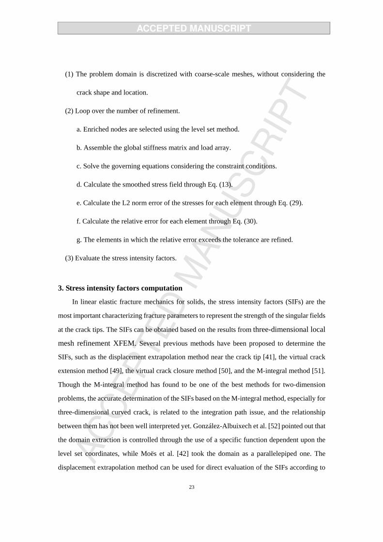
(1) The problem domain is discretized with coarse-scale meshes, without considering the

crack shape and location.

(2) Loop over the number of refinement.

a. Enriched nodes are selected using the level set method.

b. Assemble the global stiffness matrix and load array.

c. Solve the governing equations considering the constraint conditions.

d. Calculate the smoothed stress field through Eq. (13).

e. Calculate the L2 norm error of the stresses for each element through Eq. (29).

f. Calculate the relative error for each element through Eq. (30).

g. The elements in which the relative error exceeds the tolerance are refined.

(3) Evaluate the stress intensity factors.

3. Stress intensity factors computation

In linear elastic fracture mechanics for solids, the stress intensity factors (SIFs) are the

most important characterizing fracture parameters to represent the strength of the singular fields

at the crack tips. The SIFs can be obtained based on the results from three-dimensional local

mesh refinement XFEM. Several previous methods have been proposed to determine the

SIFs, such as the displacement extrapolation method near the crack tip [41], the virtual crack

extension method [49], the virtual crack closure method [50], and the M-integral method [51].

Though the M-integral method has found to be one of the best methods for two-dimension

problems, the accurate determination of the SIFs based on the M-integral method, especially for

three-dimensional curved crack, is related to the integration path issue, and the relationship

between them has not been well interpreted yet. González-Albuixech et al. [52] pointed out that

the domain extraction is controlled through the use of a specific function dependent upon the

level set coordinates, while Moës et al. [42] took the domain as a parallelepiped one. The

displacement extrapolation method can be used for direct evaluation of the SIFs according to

24

the relative crack surface displacements. Throughout this study, the displacement extrapolation

method is employed for estimating the SIFs for our 3-D numerical examples.

Nevertheless, future works would be interesting if the M1-integral method could be

integrated into the present formulation to extract the fracture parameters. In fact the authors

have made some preliminary attempts to the use of the M1-integral method for extracting the

SIFs of planar 3-D straight and curved cracks in the framework of the Lm-XFEM. The accuracy

that we have observed however does not reach our final goal as less accuracy is observed in the

SIFs exacted by the method for 3-D curved cracks, and more importantly the dependent path of

J-integral is problematic. Further developments to improve the accuracy of the SIFs using the

M1-integral method for 3-D curved cracks are thus necessary, but it would probably take much

effort in fulfilling the tasks, and in the present circumstance it is out of the scope of this

manuscript. Therefore, we have scheduled to study this discussed issue in our next manuscript

comprehensively.

In the crack-tip Cartesian coordinates, the relation between the relative displacements and

the SIFs are [54]

( )I2

1GK v

k rΔπ

=+

(32)

( )II2

1GK u

k rΔπ

=+

(33)

( )III2

1GK w

k rΔπ

=+

(34)

where G is the shearing modulus; 31

k νν−

=+

, ν is the Poisson’s ratio; r is the ray distance

from the crack front; while uΔ , vΔ , and wΔ are the relative displacements near the crack

front in the crack front Cartesian coordinates on the crack surface.

Some points in the same normal direction from the crack front on the crack surface is taken

to construct a set array ( , , )i i i ir K K KΙ ΙΙ ΙΙΙ , where ir is the distance from point i to the crack front

and iKΙ , iKΙΙ , iKΙΙΙ are the SIFs of point i . By using the least squares method to fit the set array,

the SIFs at crack front can then be determined through the following relations [55]:

25

( )2

2 2

i i i i i

i i

r r K r KK

r N rΙ Ι

Ι

−≈

−∑ ∑ ∑ ∑

∑ ∑ (35a)

( )2

2 2

i i i i i

i i

r r K r KK

r N rΙΙ ΙΙ

ΙΙ

−≈

−∑ ∑ ∑ ∑

∑ ∑

(35b)

( )2

2 2

i i i i i

i i

r r K r KK

r N rΙΙΙ ΙΙΙ

ΙΙΙ

−≈

−∑ ∑ ∑ ∑

∑ ∑

(35c)

where N is the number of chosen points in the same normal direction from the crack front on

the crack surface, 10N = is adopted in this study.

From Eq. (1), it is obvious that the relative displacements on the crack surface depend only

on the enrichment variables, so it is easy to determine the SIFs using the relative displacements

on the crack surface in the XFEM.

4. Numerical experiments and discussions

In this section, we particularly concentrate our attention on numerical experiments and

accurate investigation of the SIFs calculated by the present method. An in-house 3-D

MATLAB code for solving SIFs using the 3-D local mesh refinement XFEM with

variable-node hexahedron elements is developed. To this end, six numerical examples of planar

straight and curved cracks embedded in 3-D solids with single and mixed-mode fractures are

hence considered:

• The first three examples deal with single and mixed-mode fracture in 3-D by

considering an edge straight crack, a central straight crack and an edge inclined

straight crack.

• The last three examples deal with curved cracks in 3-D by considering a central

penny shaped crack, a central ellipse shaped crack and an edge ellipse shaped

crack.

All the numerical results are analyzed and validated against the reference solutions to show

the accuracy and effectiveness of the developed Lm-XFEM. The SIFs extracted by using the

displacement extrapolation method are then compared with analytical solutions available in

literature and the conventional XFEM with fine meshes.

26

Regarding the number of Gaussian quadrature point used in the numerical computations,

the cut or split element is divided into 12 sub-elements and each sub-element uses 4 Gaussian

points, so all of them total 48 points. For the tip element, it is divided into 18 sub-elements and

each of them uses 5 Gaussian points and thus its total is 90 points. Elements that do not contain

any crack but engage tip nodes use 4 4 4× × Gaussian points, while other elements use 2 2 2× ×

points.

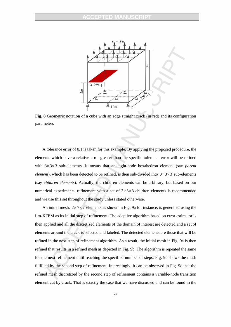
4.1 An edge straight crack

A cube of size 10m 10m 10m× × containing an edge straight crack as schematically

depicted in Fig. 8 is considered. A crack length of 2.5m as shown in the figure is taken. The top

surface of the cube is subjected to a uniform traction of 1Paσ = while the bottom surface is

constrained in all directions. The following material parameters, the Young’s modulus

206GPaE = and the Poisson ratio 0.3ν = , are used throughout the study if not specified

otherwise.

Under the plane strain condition, the analytical solution of this edge crack problem for

0.6dl≤ is given by [56]

refI

dK d Fl

σ π ⎛ ⎞= ⎜ ⎟⎝ ⎠

(36)

with

2 3 4

1.12 0.231 10.55 21.72 30.39d d d dFl l l l

⎛ ⎞ ⎛ ⎞ ⎛ ⎞= − + − +⎜ ⎟ ⎜ ⎟ ⎜ ⎟⎝ ⎠ ⎝ ⎠ ⎝ ⎠

(37)

where d denotes the crack length while l is the length of the cube along the crack direction.

For this example, only mode-I SIF is extracted using the displacement extrapolation

method. The mode-I SIF is then estimated for each step of refinement using the Lm-XFEM and

is compared with the results derived from the conventional XFEM as well as analytical

solutions. The study is to show the accuracy of the developed Lm-XFEM in determining the

SIFs of a planar 3-D edge straight crack in a elastic cube.

27

Fig. 8 Geometric notation of a cube with an edge straight crack (in red) and its configuration

parameters

A tolerance error of 0.1 is taken for this example. By applying the proposed procedure, the

elements which have a relative error greater than the specific tolerance error will be refined

with 3 3 3× × sub-elements. It means that an eight-node hexahedron element (say parent

element), which has been detected to be refined, is then sub-divided into 3 3 3× × sub-elements

(say children elements). Actually, the children elements can be arbitrary, but based on our

numerical experiments, refinement with a set of 3 3 3× × children elements is recommended

and we use this set throughout the study unless stated otherwise.

An initial mesh, 7 7 7× × elements as shown in Fig. 9a for instance, is generated using the

Lm-XFEM as its initial step of refinement. The adaptive algorithm based on error estimator is

then applied and all the discretized elements of the domain of interest are detected and a set of

elements around the crack is selected and labeled. The detected elements are those that will be

refined in the next step of refinement algorithm. As a result, the initial mesh in Fig. 9a is then

refined that results in a refined mesh as depicted in Fig. 9b. The algorithm is repeated the same

for the next refinement until reaching the specified number of steps. Fig. 9c shows the mesh

fulfilled by the second step of refinement. Interestingly, it can be observed in Fig. 9c that the

refined mesh discretized by the second step of refinement contains a variable-node transition

element cut by crack. That is exactly the case that we have discussed and can be found in the

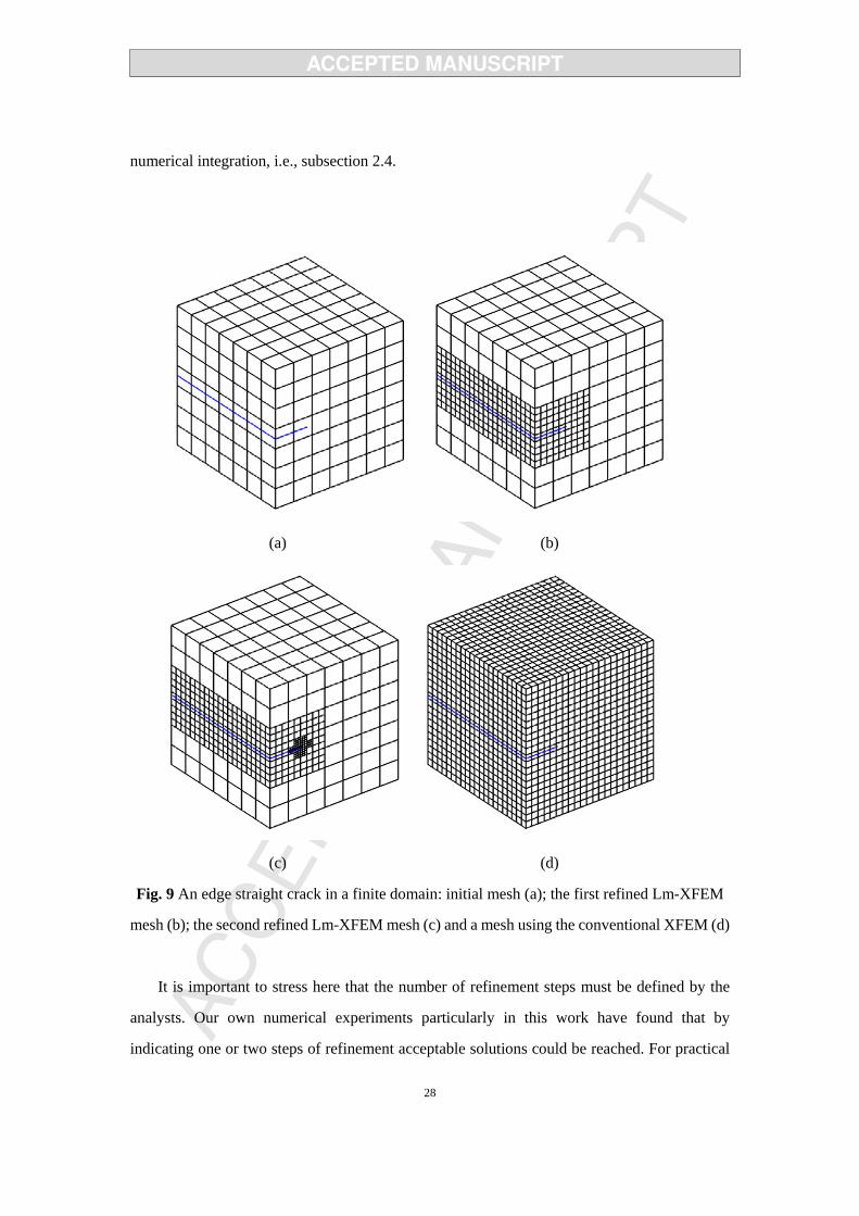
28

numerical integration, i.e., subsection 2.4.

(a) (b)

(c) (d)

Fig. 9 An edge straight crack in a finite domain: initial mesh (a); the first refined Lm-XFEM

mesh (b); the second refined Lm-XFEM mesh (c) and a mesh using the conventional XFEM (d)

It is important to stress here that the number of refinement steps must be defined by the

analysts. Our own numerical experiments particularly in this work have found that by

indicating one or two steps of refinement acceptable solutions could be reached. For practical

29

purposes however at least two steps of refinement or even more is recommended. Determining

an appropriate number of refinement steps for each particular problem is trivial.

The subsequent numerical investigations, one or two steps of refinement have been

examined and studied. For comparison, the entire computational domain using small-scale

elements as shown in Fig. 9d is also added, which is derived from the conventional XFEM. All

the meshes sketched in Fig. 9 are very interesting since it reveals the advantages of the

developed Lm-XFEM over the traditional XFEM. It is because the refined mesh deals with the

region that only covers the crack and the areas far from the crack do not take into account. In

addition, the number of elements or nodes gained by the conventional XFEM is much larger

than that discretized by the Lm-XFEM. This issue is addressed and illustrated in the following

numerical results.

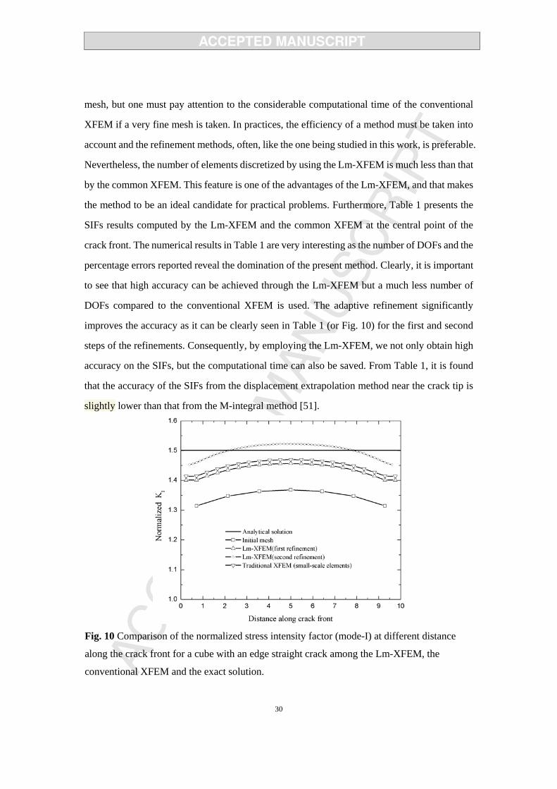
For convenience in representing the numerical results, the SIFs are normalized by

* /I IK K dσ π= . Fig. 10 shows the calculated results of *IK at crack front with respect to

different distances along crack front using the Lm-XFEM and the conventional XFEM with a

fine mesh, e.g., 21 21 21× × elements. Unlike the edge crack in 2-D solids where only one crack

tip exists, the edge crack in 3-D is however more complicated than that as there exists a crack

front (not a crack tip). The *IK at certain points at the crack front, different locations, are

computed and presented here. Therefore, the numerical results plotted in Fig. 10 represent the

*IK at different distances along the crack front. The *

IK results gained by the Lm-XFEM

approach well to the exact solutions. Not surprisingly, the initial results using the initial mesh

exhibit so poor but the accuracy of the *IK increases significantly after each step of refinement,

which exactly reflects the desirable characteristics of the developed Lm-XFEM. In addition, the

accuracy of the SIFs calculated by the standard XFEM with a fine mesh is far way from the

exact solutions as compared with that derived from the second step of refinement using the

Lm-XFEM. From the results sketched in Fig. 10, one can see that the SIFs measured at different

locations along the crack front are slightly different.

There is another interesting point regarding the standard XFEM that must be discussed here.

It is, in general, the accuracy of the standard XFEM can be further improved by taking a finer

30

mesh, but one must pay attention to the considerable computational time of the conventional

XFEM if a very fine mesh is taken. In practices, the efficiency of a method must be taken into

account and the refinement methods, often, like the one being studied in this work, is preferable.

Nevertheless, the number of elements discretized by using the Lm-XFEM is much less than that

by the common XFEM. This feature is one of the advantages of the Lm-XFEM, and that makes

the method to be an ideal candidate for practical problems. Furthermore, Table 1 presents the

SIFs results computed by the Lm-XFEM and the common XFEM at the central point of the

crack front. The numerical results in Table 1 are very interesting as the number of DOFs and the

percentage errors reported reveal the domination of the present method. Clearly, it is important

to see that high accuracy can be achieved through the Lm-XFEM but a much less number of

DOFs compared to the conventional XFEM is used. The adaptive refinement significantly

improves the accuracy as it can be clearly seen in Table 1 (or Fig. 10) for the first and second

steps of the refinements. Consequently, by employing the Lm-XFEM, we not only obtain high

accuracy on the SIFs, but the computational time can also be saved. From Table 1, it is found

that the accuracy of the SIFs from the displacement extrapolation method near the crack tip is

slightly lower than that from the M-integral method [51].

Fig. 10 Comparison of the normalized stress intensity factor (mode-I) at different distance

along the crack front for a cube with an edge straight crack among the Lm-XFEM, the

conventional XFEM and the exact solution.

31

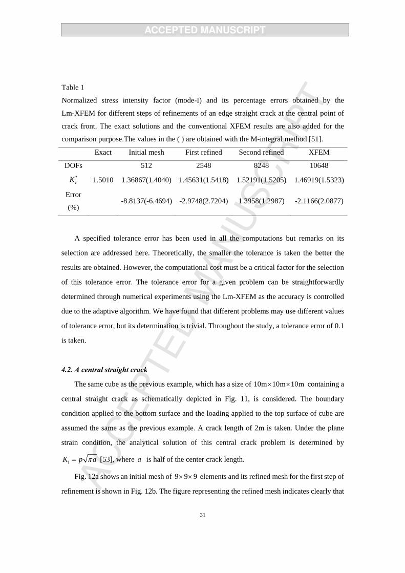
Table 1

Normalized stress intensity factor (mode-I) and its percentage errors obtained by the

Lm-XFEM for different steps of refinements of an edge straight crack at the central point of

crack front. The exact solutions and the conventional XFEM results are also added for the

comparison purpose.The values in the ( ) are obtained with the M-integral method [51].

Exact Initial mesh First refined Second refined XFEM

DOFs 512 2548 8248 10648 *IK 1.5010 1.36867(1.4040) 1.45631(1.5418) 1.52191(1.5205) 1.46919(1.5323)

Error

(%) -8.8137(-6.4694) -2.9748(2.7204) 1.3958(1.2987) -2.1166(2.0877)

A specified tolerance error has been used in all the computations but remarks on its

selection are addressed here. Theoretically, the smaller the tolerance is taken the better the

results are obtained. However, the computational cost must be a critical factor for the selection

of this tolerance error. The tolerance error for a given problem can be straightforwardly

determined through numerical experiments using the Lm-XFEM as the accuracy is controlled

due to the adaptive algorithm. We have found that different problems may use different values

of tolerance error, but its determination is trivial. Throughout the study, a tolerance error of 0.1

is taken.

4.2. A central straight crack

The same cube as the previous example, which has a size of 10m 10m 10m× × containing a

central straight crack as schematically depicted in Fig. 11, is considered. The boundary

condition applied to the bottom surface and the loading applied to the top surface of cube are

assumed the same as the previous example. A crack length of 2m is taken. Under the plane

strain condition, the analytical solution of this central crack problem is determined by

K p aπΙ = [53], where a is half of the center crack length.

Fig. 12a shows an initial mesh of 9 9 9× × elements and its refined mesh for the first step of

refinement is shown in Fig. 12b. The figure representing the refined mesh indicates clearly that

32

only region around the crack is refined, and this is a great advantage of the method, especially

for 3-D problems where the computational efficiency takes place as a critical factor.

The SIFs are calculated using the displacement extrapolation method for only one crack

front due to the symmetric configuration. The computed SIFs at different distance along the

crack front for the central crack are visualized in Fig. 13, showing a comparison between the

present results with respect to the conventional XFEM solution using a fine mesh of

27 27 27× × elements. Note that the SIFs reported here represent their real values and are not

normalized. The SIFs based on the initial mesh is again found to be inaccurate whereas that

achieved by the Lm-XFEM approach well to the exact solutions [53] and match well with the

common XFEM results. We perform only one step of refinement since its results obtained are

adequately accurate, and further steps of refinement may not be necessary. However, as stated

above higher numbers of refinement steps may be necessary, especially for practical problems.

Fig. 11 Geometric notation of a cube with a central straight crack and its configuration

parameters showing the boundary and loading conditions

33

(a) (b)

Fig. 12 A central straight crack in a finite domain: Initial mesh (a); and 3 3 3× × refined

Lm-XFEM mesh (b).

Fig. 13 Comparison of the stress intensity factor (mode-I) at different distance along the crack

front for a cube with a central straight crack among the Lm-XFEM, the traditional XFEM and

the exact solution.

34

4.3. A mixed-mode edge inclined straight crack

This example is mainly devoted to study the mixed-mode fracture problem in 3-D planar

cracks using the present method. It is accomplished by considering an edge inclined straight

crack in a plate under uniform tension as depicted in Fig.14. The size of the plate is

10m 25m 25m× × and the angle of the inclined crack is set to be 45 . The material parameters

and the boundary conditions as well as the loading conditions are taken the same as the previous

examples. The length of the crack front is equal to the size of the body, i.e., 25m, see Fig. 14,

while the crack length is indicated by a as shown in the same figure. Different crack lengths

are studied by varying a from 3 to 5, and the corresponding SIFs for each a are then estimated,

respectively.

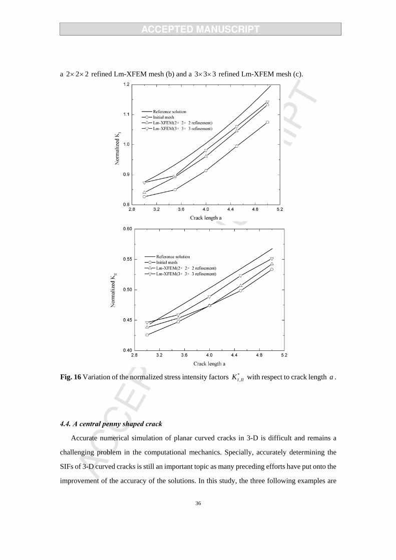
In this example, two different sets of subdivisions elements or children elements e. g.,

2 2 2× × and 3 3 3× × , are considered. The use of different sets of subdivided elements is to

clarify the effect of the number of subdivisions per element on the accuracy of the SIFs. The

same initial mesh of 5 11 11× × elements as sketched in Fig. 15a is taken, and the refined meshes

derived from the Lm-XFEM for the two subdivisions of 2 2 2× × and 3 3 3× × children

elements are shown in Figs. 15b and 15c, respectively. Note that the refined meshes for 3ma = ,

for instance, is performed. The SIFs are calculated by the displacement extrapolation method

with one step of refinement for different values of the parameter a . They are then normalized

by *, , /I II I IIK K dσ π= and eventually depicted in Figs. 16a (mode-I) and 16b (mode-II),

respectively. The normalized mode-I and mode-II are estimated at a central position of the

crack front. Numerical results for each set of subdivided children elements are calculated for

different values of a . Compared with the reference solutions given by Institute of China

Aeronaut [57], the Lm-XFEM using the subdivided set of 3 3 3× × children elements offers the

*,I IIK more accurate than that utilizing the subdivided set of 2 2 2× × elements. In other words,

the SIFs derived from the 3 3 3× × children elements approach to the exact solutions better than

that from 2 2 2× × elements. More interestingly, it is very important to note that the effect of the

crack length on the *,I IIK is significant. The *

,I IIK SIFs increase with increasing the crack length,

35

as a result of the finite size effect in fracture mechanic problems.

Fig. 14 Schematic configuration of an edge inclined straight crack in a finite domain showing

the boundary and loading conditions

(a) (b) (c)

Fig. 15 An edge inclined crack in a finite domain for a crack-length of 3ma = : Initial mesh (a);

36

a 2 2 2× × refined Lm-XFEM mesh (b) and a 3 3 3× × refined Lm-XFEM mesh (c).

Fig. 16 Variation of the normalized stress intensity factors *,I IIK with respect to crack length a .

4.4. A central penny shaped crack

Accurate numerical simulation of planar curved cracks in 3-D is difficult and remains a

challenging problem in the computational mechanics. Specially, accurately determining the

SIFs of 3-D curved cracks is still an important topic as many preceding efforts have put onto the

improvement of the accuracy of the solutions. In this study, the three following examples are

37

devoted to illustrate the applicability of the developed Lm-XFEM in simulating 3-D curved

cracks. The accuracy of the SIFs are hence examined and validated.

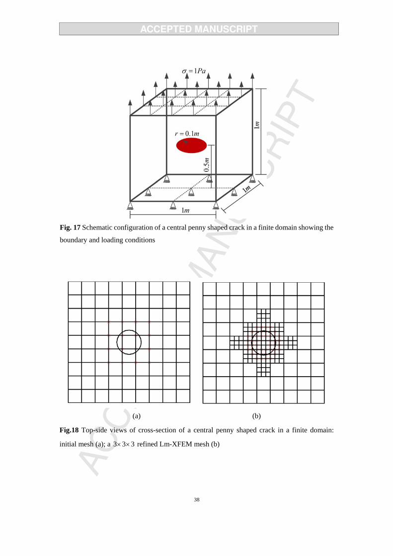
We start by examining a cuboid of size 1m 1m 1m× × containing a penny shaped crack as

shown in Fig.17. The radius of the penny is taken as 0.1mr = . The analytical solutions of this

problem are available in Ref. [58], i.e., 2 rK σπΙ = and 0K KΙΙ ΙΙΙ= = . Similarly, the

Lm-XFEM is applied to solve this example. By accomplishing that, an initial mesh of 9 9 9× ×

elements is discretized using the Lm-XFEM. Fig. 18a shows the top-side view of cross-section

for the initial mesh of the penny shaped crack while its refined mesh is sketched in Fig. 18b,

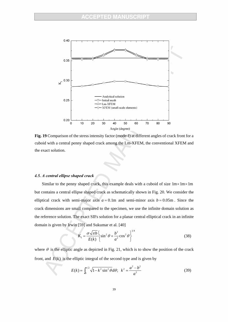
also the top-side view of cross-section. Different from the previous examples, the SIFs for this

penny shaped crack are however estimated at different angles and their computed results are

plotted in Fig. 19. Note that the SIFs reported here represent their real values and are not

normalized. For verification, results obtained by the traditional XFEM with a fine mesh are also

added. The present results indicate the accuracy of the Lm-XFEM as its obtained SIFs approach

well to the exact solutions. The SIFs obtained by the traditional XFEM using a fine mesh of

27 27 27× × elements are in a good agreement with the Lm-XFEM as clearly shown in the

figure. Even through the accuracy of the SIFs is equivalent but one must note that the great

difference distinguishing between the Lm-XFEM and the traditional XFEM is the

computational cost and the number of DOFs that are being used for the implementation. The

Lm-XFEM with refinement and adaptive algorithm always offers a great advantage over the

traditional XFEM to these facts. Nonetheless, the SIFs of this penny shaped crack behave an

oscillation around the exact solutions for some angles at the crack front. However, the error on

the numerical results obtained by the Lm-XFEM with respect to the exact solutions is small. It

is noted that the “bump” of the SIFs obtained by the XFEM in Fig. 19 can be caused by the

finite domain used in the computations. By increasing the computational domain the error can

substantially be reduced.

38

Fig. 17 Schematic configuration of a central penny shaped crack in a finite domain showing the

boundary and loading conditions

(a) (b)

Fig.18 Top-side views of cross-section of a central penny shaped crack in a finite domain:

initial mesh (a); a 3 3 3× × refined Lm-XFEM mesh (b)

39

Fig. 19 Comparison of the stress intensity factor (mode-I) at different angles of crack front for a

cuboid with a central penny shaped crack among the Lm-XFEM, the conventional XFEM and

the exact solution.

4.5. A central ellipse shaped crack

Similar to the penny shaped crack, this example deals with a cuboid of size 1m 1m 1m× ×

but contains a central ellipse shaped crack as schematically shown in Fig. 20. We consider the

elliptical crack with semi-major axis 0.1ma = and semi-minor axis 0.05mb = . Since the

crack dimensions are small compared to the specimen, we use the infinite domain solution as

the reference solution. The exact SIFs solution for a planar central elliptical crack in an infinite

domain is given by Irwin [59] and Sukumar et al. [40] 1 42

2 22sin cos

( )b bK

E k aσ π θ θΙ

⎧ ⎫= +⎨ ⎬

⎩ ⎭ (38)

where θ is the elliptic angle as depicted in Fig. 21, which is to show the position of the crack

front, and ( )E k is the elliptic integral of the second type and is given by

2 22 2 2 220

( ) 1 sin ; a bE k k d ka

πθ θ −

= − =∫ (39)

40

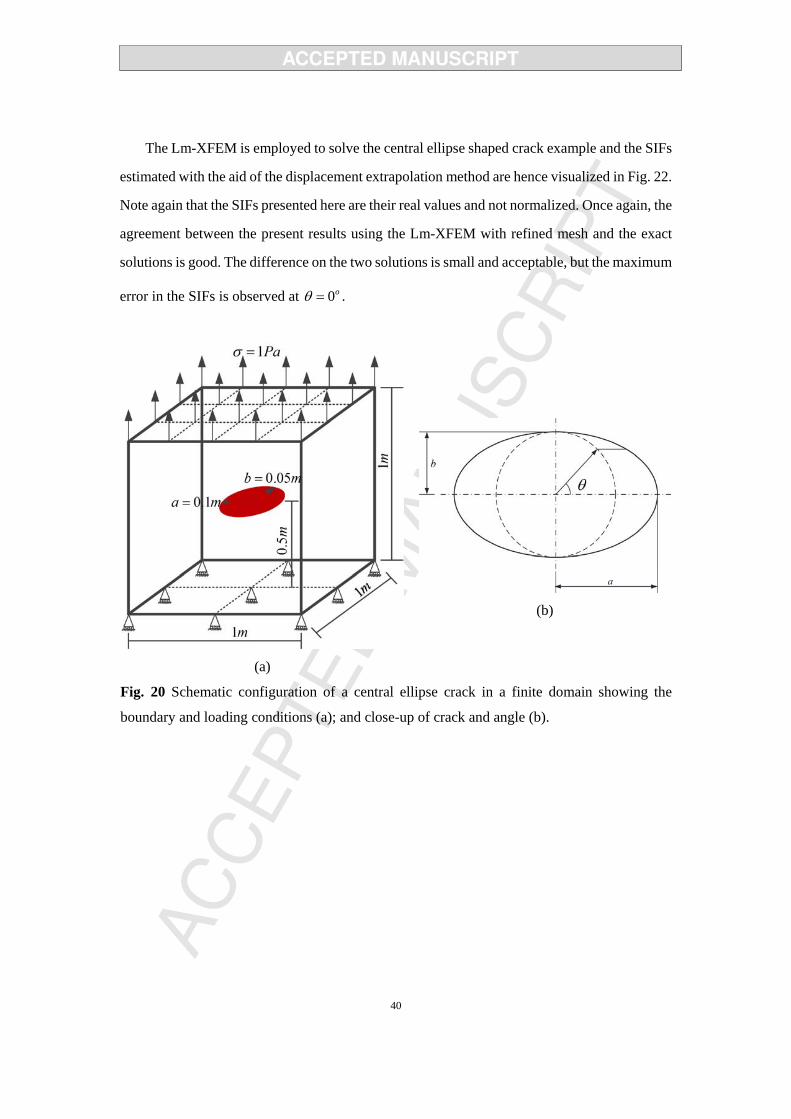
The Lm-XFEM is employed to solve the central ellipse shaped crack example and the SIFs

estimated with the aid of the displacement extrapolation method are hence visualized in Fig. 22.

Note again that the SIFs presented here are their real values and not normalized. Once again, the

agreement between the present results using the Lm-XFEM with refined mesh and the exact

solutions is good. The difference on the two solutions is small and acceptable, but the maximum

error in the SIFs is observed at 0oθ = .

(a)

(b)

Fig. 20 Schematic configuration of a central ellipse crack in a finite domain showing the

boundary and loading conditions (a); and close-up of crack and angle (b).

41

Fig. 21 Geometric definitions for a central ellipse shaped crack

Fig. 22 Mode-I stress intensity factor at different angles of crack front for a cuboid with a

central ellipse shaped crack obtained by the Lm-XFEM.

42

4.6. An edge ellipse shaped crack

Last example deals with an edge ellipse shaped crack in a plate under uniform tension as

shown as Fig. 23. The size of the plate is set to be 10m 4m 10m× × and the elliptical crack’s

semi-major axis 2mc = and semi-minor axis 1ma = . The body is also subjected to a uniform

traction of 1Paσ = and the bottom surface is also constrained in all the direction. This problem

has been analyzed previously by different methods and numerical solutions are readily

available in the literature. Among the solutions available, the one derived from Newman and

Raju [60] is widely used. The stress intensity factors are normalized by

* /I IaK K ac

Qπσ= (40)

with 1.65

1.65

1 1.464( / ) if ( / ) 11 1.464( / ) if ( / ) 1

a c a cQ

c a c a⎧ + ≤

= ⎨+ >⎩

(41)

We use a set of initial mesh of 5 11 11× × elements to this example. To show the effect of

the number of subdivision elements of children elements on the SIFs, we hence consider two

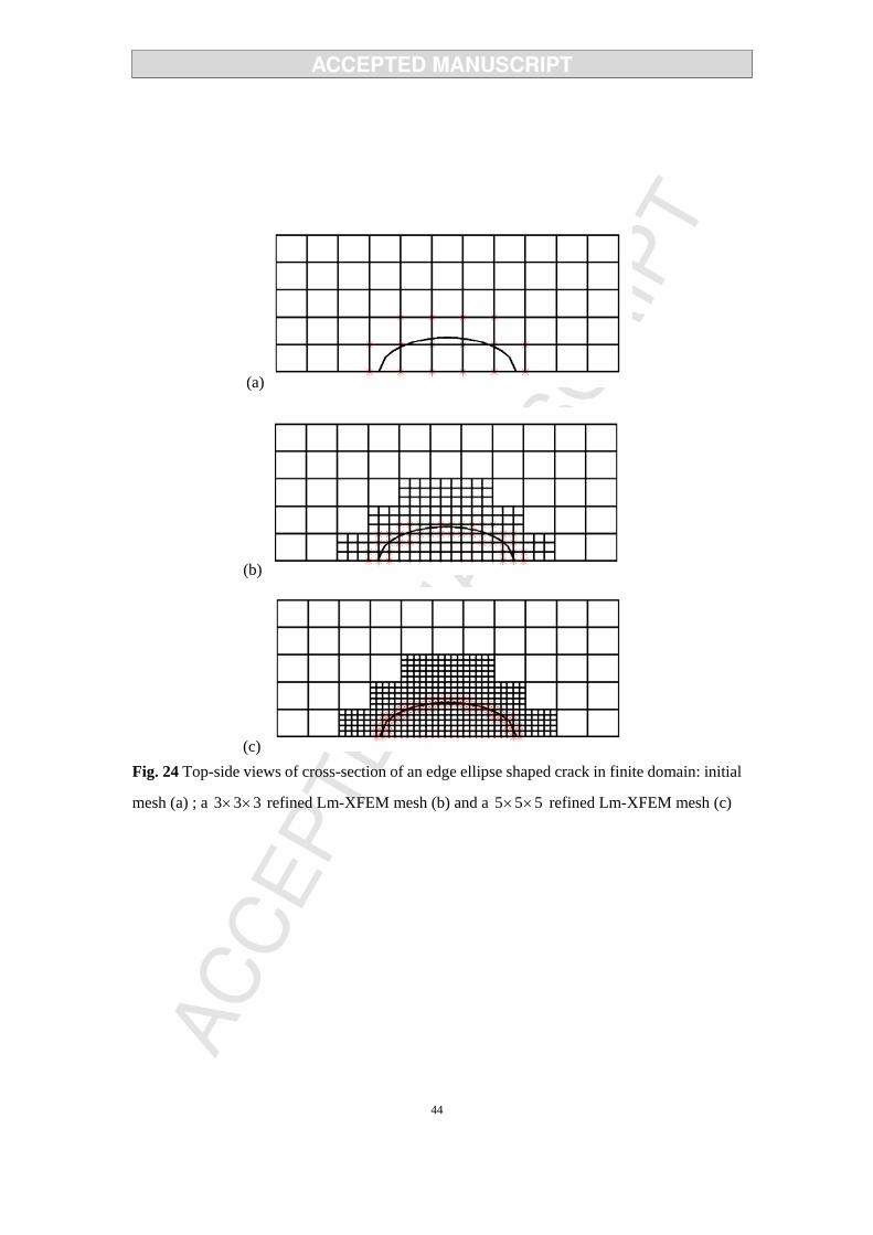
different sets of the number of subdivision, for instance, 3 3 3× × and 5 5 5× × . Fig. 24a

sketches the initial mesh of edge ellipse shaped crack. Note that the top-side view of

cross-section is shown due to the convenience in the representation of the 3-D crack. Figs. 24b

and 24c, respectively, depict the refined meshes of the cracks using the suggested number of

subdivision elements discretized by the adaptive refinement Lm-XFEM. The numerical results

of the SIFs estimated based on the two given sets of children elements are then shown in Fig. 25.

Similarly, the common XFEM with fine mesh and exact solutions [60] are also plotted in the

same figure for the validation purpose. The present results indicate clearly that the Lm-XFEM

with 5 5 5× × subdivision elements can offer a good accuracy as their SIFs are closer to the

exact solutions than other reference solutions. However, the cost that devotes to the use of a

higher number of subdivision elements is high.

43

(a)

(b)

Fig. 23 Geometric notation of an edge ellipse shaped crack in finite domain and its

configuration parameters (a); and close-up of crack and angle (b).

44

(a)

(b)

(c) Fig. 24 Top-side views of cross-section of an edge ellipse shaped crack in finite domain: initial

mesh (a) ; a 3 3 3× × refined Lm-XFEM mesh (b) and a 5 5 5× × refined Lm-XFEM mesh (c)

45

Fig. 25 Comparison of the normalized stress intensity factor (mode-I) at different angles along

the crack front for an edge ellipse shaped crack among the Lm-XFEM, the conventional XFEM

and the exact solution.

5. Conclusions and outlook

A novel 3-D adaptive local mesh refinement extended finite element method (Lm-XFEM)

using hexahedron elements for the accurate computation of the stress intensity factors of

planar straight and curved cracks in solids is presented. This 3-D approach, on one hand,

engages a posteriori recovery-based error estimation to detect all elements that shall be

refined in the next refinement step, the variable-node hexahedron elements, on the other hand,

are adopted to treat the mismatching problems caused by different scale-meshes. The strategy

presenting here reflects the robustness of an effective numerical method as the fine-scale mesh

is only tackled to where it is required. The numerical results of the SIFs for single and

mixed-mode 3-D crack problems obviously show the effectiveness and high accuracy of the

proposed Lm-XFEM method.

We have found through the numerical investigation that the variable-node hexahedron

element based on the generic point interpolation is effective and straightforward in treating the

46

mismatching problems of different meshes. The adaptive algorithm reflects the region where

fine meshes are required to be refined, which makes the method possible to improve the

accuracy of the solutions around the cracks. Moreover, the Lm-XFEM carries with less DOFs

than those through the XFEM.

In XFEM setting, the mesh is independent of crack geometry, and small cracks in the

analysis of large structures can be considered by employing the coupling meshes scheme. The

Lm-XFEM proposed thus is an efficient numerical method, and is particularly suitable for

modeling cracks embedded in large structures. Due to the accuracy, simplicity, and the

flexibility of the Lm-XFEM, we believe that the method presented here is well and ideally

suited for engineering analysis. The proposed formulation is general and its extension to other

complex problems is possible. Multiple cracks, crack growth in 3-D problems, and non-planar

3-D cracks are those that are very interesting to study. We may further develop it for modeling

cracks in advanced composite materials, e.g., layered functionally graded materials [51], or to

industrial applications problems. Those works inherently are challenging but would be an

interesting subject for our future research directions.

More specifically, the multiple branched cracks can be modelled by introducing a junction

function to the present displacement approximation. The presented formulas in this paper can

be further developed for solving non-planar 3-D cracks as well. In the XFEM, the crack surface

is often described through the level sets. Compared with planar 3-D cracks, representing

non-planar 3-D cracks with the level set method would be more complicated. The crack growth

in 3-D problems can be modelled by introducing appropriate crack propagation criteria into the

present formulation. The high-efficient updating algorithm of level sets and 3-D crack growth

algorithm are two key issues in the analysis of 3-D crack propagation. Some scholars

successfully modelled 3-D crack propagation with the XFEM, see for instance Refs. [42, 61].

In addition, the discretization of tetrahedral elements is common in general engineering

practice. The variable-node tetrahedral elements can be devised based on the generic point

interpolation with an arbitrary number of nodes on each of their faces, thus the proposed

method can be applied to complex problems discretizated with tetrahedral elements.

Nonetheless, the current version of the developed 3-D Lm-XFEM employs the

displacement extrapolation method to extract the SIFs. As have been shown in the subsequent

47

numerical examples, the current version works quite well for both straight and curved cracks as

well as single and mixed-mode fractures. Further development by taking the M-integral method

and integrating it into the Lm-XFEM is necessary and important. To this end, the accuracy of

the SIFs and the path independent problem are two important issues that must be taken into

consideration.

Acknowledgements

This work was supported by the Grant-in-Aid for Scientific Research - Japan Society for the

Promotion of Sciences (JSPS); the National Natural Science Foundation of China (Grant No.

51179063); and the National Sci-Tech Support Plan of China (Grant No. 2015BAB07B10). The

financial supports are gratefully acknowledged.

References

[1] P.A. Guidault, O. Allix, L. Champaney, J.P. Navarro, A two-scale approach with

homogenization for the computation of cracked structures, Computers and Structures

85(2007)1360-1371.

[2] M. Holl, S. Loehnert, P. Wriggers, An adaptive multiscale method for crack propagation

and crack coalescence, Internat. J. Numer. Methods Engrg. 93(2013)23-51.

[3] C. Prange, S. Loehnert, P. Wriggers, Error estimation for crack simulations using the XFEM,

Internat. J. Numer. Methods Engrg. 91(2012)1459-1474.

[4] P.A. Guidault, Q. Allix, L. Champaney, C. Cornuault, A multiscale extended finite element

method for crack propagation, Comput. Methods Appl. Mech. Engrg. 197(2008)381-399.

[5] S. Loehnert, T. Belytschko, A multiscale projection method for macro/microcrack

simulations, Internat. J. Numer. Methods Engrg. 71(2007)1466-1482.

[6] A. de Boer, A.H. van Zuijlen, H. Bijl, Review of coupling methods for nonmatching meshes,

Comput. Methods Appl. Mech. Engrg. 196(2007)1515-1525.

[7] M.A. Puso, A 3D mortar method for solid mechanics, Internat. J. Numer. Methods

Engrg.59(2002)315-336.

[8] H.B. Dhia, G. Rateau, The Arlequin method as a flexible engineering design tool, Internat. J.

48

Numer. Methods Engrg. 62(2005)1442-1462.

[9] T. Belytschko, S. Loehnert, J.H. Song, Multiscale aggregating discontinuities: A method for

circumventing loss of material stability, Internat. J. Numer. Methods Engrg.

73(2008)869-894.

[10] N. Moës, J. Dolbow, T. Belytshko, A finite element for crack growth without remeshing,

Internat. J. Numer. Methods Engrg. 46(1999)131-150.

[11] J.H. Song, T. Belytschko, Multiscale aggregating discontinuities method for micro–macro

failure of composites, Composites Part B: Engineering 40(2009)417-426.

[12] T. Belytschko, J.H. Song, Coarse-graining of multiscale crack propagation, Internat. J.

Numer. Methods Engrg. 81(2010)537-563.

[13] J.A. Plews, C.A. Duarte, Bridging multiple structural scales with a generalized finite

element method, Internat. J. Numer. Methods Engrg. 102(2015)180-201.

[14] T. Hettich, A. Hund, E. Ramm, Modeling of failure in composites by X-FEM and level sets

within a multiscale framework, Comput. Methods Appl. Mech. Engrg.197(2008)414-424.

[15] E. Pierrès, M.C. Baietto, A. Gravouil, A two-scale extended finite element method for

modelling 3D crack growth with interfacial contact, Comput. Methods Appl. Mech. Engrg.

199(2010)1165-1177.

[16] A. Sarhangi Fard, M.A. Hulsen, H.E.H. Meijer, N.M.H. Famili, P.D. Anderson, Adaptive

non-conformal mesh refinement and extended finite element method for viscous flow

inside complex moving geometries, International Journal for Numerical Methods in Fluids

68(2012)1031-1052.

[17] A. Byfut, A. Schröder, hp-adaptive extended finite element method, Internat. J. Numer.

Methods Engrg. 89(2012)1392-1418.

[18] S. Loehnert, C. Prange, P. Wriggers, Error controlled adaptive multiscale XFEM

simulation of cracks, International Journal of Fracture 178(2012)147-156.

[19] D. Sohn, J.H. Lim, S. Im, An efficient scheme for coupling dissimilar hexahedral meshes

with the aid of variable-node transition elements, Advances in Engineering Software

65(2013)200-215.

[20] S. Kumar, I.V. Singh, B.K. Mishra, A homogenized XFEM approach to simulate fatigue

crack growth problems, Computers and Structures 150 (2015) 1-22

49

[21] S. Kumar, I.V. Singh, B.K. Mishra, T. Rabczuk. Modeling and simulation of kinked cracks

by virtual node XFEM, Computer Methods in Applied Mechanics and Engineering.

283(2015)1425-1466.

[22] J.H. Lim, D. Sohn, S. Im, Variable-node element families for mesh connection and

adaptive mesh computation, Structural Engineering and Mechanics 43(2012)349-370.

[23] Q.T. Bui, Ch. Zhang, Extended finite element simulation of stationary dynamic cracks in

piezoelectric solids under impact loading, Computational Materials Science

62(2012)243-257.

[24] Q.T. Bui, Ch. Zhang, Analysis of generalized dynamic intensity factors of cracked

magnetoelectroelastic solids by X-FEM, Finite Elem. Anal. Des. 69(2013)19-36.

[25] P. Liu, T.T. Yu, Q.T. Bui, Ch. Zhang, Transient dynamic crack analysis in

non-homogeneous functionally graded piezoelectric materials by the X-FEM,

Computational Materials Science 69(2013)542-558.

[26] P. Liu, T.T. Yu, Q.T. Bui, Ch. Zhang, Y.P. Xu, C.W. Lim, Transient thermal shock fracture

analysis of functionally graded piezoelectric materials by the extended finite element

method, International Journal of Solids and Structures 51(2014)2167-2182.

[27] T.T. Yu, Q.T. Bui, P. Liu, Ch. Zhang, S. Hirose, Interfacial dynamic impermeable cracks

analysis in dissimilar piezoelectric materials under coupled electromechanical loading

with the extended finite element method, International Journal of Solids and Structures,

67-68(2015)205-218.

[28] K. Sharma, Q.T. Bui, Ch. Zhang, R.R. Bhargava, Analysis of a subinterface crack in

piezoelectric bimaterials with the extended finite element method, Engineering Fracture

Mechanics 104(2013)114-139.

[29] S. Bhattacharya, I.V. Singh, B.K. Mishra, Q.T. Bui, Fatigue crack growth simulations of

interfacial cracks in bi-layered FGMs using XFEM, Comput. Mech. 52(2013)799-814.

[30] X.D. Zhang, Q.T. Bui, A fictitious crack XFEM with two new solution algorithms for

cohesive crack growth modeling in concrete structures, Engineering Computations

32(2015)473-497.

[31] T.T. Yu, Q.T. Bui, P. Liu, S. Hirose, A stabilized discrete shear gap extended finite

element for the analysis of cracked Reissner-Mindlin plate vibration problems involving

50

distorted mesh, International Journal of Mechanics and Materials in Design 12 (2016)

85-107.

[32] P. Liu, T.Q. Bui, D. Zhu, T.T. Yu, J.W. Wang, S.H. Yin, S. Hirose, Buckling failure

analysis of cracked functionally graded plates by a stabilized discrete shear gap extended

3-node triangular plate element. Composites Part B: Engineering 77 (2015) 179-193.

[33] L. Shi, T.T. Yu, T.Q. Bui, Numerical modeling of hydraulic fracturing in rock mass by

XFEM. Soil Mechanics and Foundation Engineering 52 (2015) 74-83.

[34] Z. Kang, T.Q. Bui, D.D. Nguyen, T. Saitoh, S. Hirose, An extended

consecutive-interpolation quadrilateral element (XCQ4) applied to linear elastic fracture

mechanics Acta Mechanica 226 (2015) 3991-4015.

[35] H. Pathak, A. Singh, I.V. Singh, S. K. Yadav, A simple and efficient XFEM approach for

3-D cracks simulations, International Journal of Fracture. 181(2013) 189-208.

[36] H. Pathak, A. Singh, I.V. Singh, S. K. Yadav, Fatigue crack growth simulations of 3-D

linear elastic cracks under thermal load by XFEM, Frontiers of Structural and Civil

Engineering, 9(2015)359-382.

[37] H. Pathak, A. Singh, I.V. Singh, Fatigue crack growth simulations of 3-D problems using

XFEM, International Journal of Mechanical Sciences 76(2013)112-131.

[38] K. Sharma, I.V. Singh, B.K. Mishra, S.K. Maurya,Numerical Simulation of Semi-elliptical

axial crack in pipe bend using XFEM, Journal of Solid Mechanics 6(2014) 208-228.

[39] O.C. Zienkiewicz, J.Z. Zhu. A simple error estimator and adaptive procedure for practical

engineering analysis. Internat. J. Numer. Methods Engrg. 24 (1987) 337-357.

[40] N. Sukumar, N. Moës, B. Moran, T. Belytschko, Extended finite element method for

three-dimensional crack modeling, Internat. J. Numer. Methods Engrg.

48(2000)1549-1570.

[41] L.S. Chen, J.H. Kuang, A modified linear extrapolation formula for determination of stress

intensity factors, International Journal of Fracture 54(1991)R3-R8.

[42] N. Moës, A. Gravouil, T. Belytschko, Non-planar 3D crack growth by the extended finite

element and level sets—Part I: Mechanical model, Internat. J. Numer. Methods Engrg.

53(2002)2549-2568.

[43] P. Laborde, J. Pommier, Y. Renard, M. Salaün, High order extended finite element

51

method for cracked domains, Int. J. Numer. Meth. Engng. 64(2005)354-381.

[44] T.P. Fries, A corrected XFEM approximation without problems in blending elements, Int.

J. Numer. Meth. Engng. 75(2008)503-532.

[45] E. Chahine, P. Laborde, Y. Renard, Crack tip enrichment in the XFEM using a cutoff

function, Int. J. Numer. Meth. Engng. 75(2008)629-646.

[46] R. Gracie, H. Wang, T. Belytschko, Blending in the extended finite element method by

discontinuous Galerkin and assumed strain methods, Int. J. Numer. Meth. Engng. 74(2008)

1645-1669.

[47] J.E. Tarancón, A. Vercher, E. Giner, F.J. Fuenmayor, Enhanced blending elements for

XFEM applied to linear elastic fracture mechanics, Int. J. Numer. Meth. Engng. 77(2009)

126-148.

[48] J. Chessa, H. Wang, T. Belytschko, On the construction of blending elements for local

partition of unity enriched finite elements, Int. J. Numer. Meth. Engng.

57(2003)1015-1038.

[49] D.M. Parks, A stiffness derivative finite element technique for determination of crack tip

stress intensity factors, International Journal of Fracture Mechanics 10(1974)487-502.

[50] E.F. Rybicki, M.F. Kanninen, A finite element calculation of stress intensity factors by a

modified crack closure integral, Engineering Fracture Mechanics 9(1977)931-938.

[51] M. Gosz, B. Moran, An interaction energy integral method for computation of

mixed-mode stress intensity factors along non-planar crack fronts in three dimensions,

Engineering Fracture Mechanics 69(2002)299-319.

[52] V.F. González-Albuixech, E. Giner, J.E. Tarancón, F.J. Fuenmayor, A. Gravouil,

Convergence of domain integrals for stress intensity factor extraction in 2-D curved cracks

problems with the extended finite element method, Internat. J. Numer. Methods Engrg.

94(2013)740-757.

[53] T.L. Anderson, Fracture Mechanics, Fundamentals and Applications (Second edition).

CRC press, New York,1995.

[54] H. Liebowitz, G.C. Sih. Mathematical Theories of Brittle Fracture. Academic Press, New

York,1968.

[55] D. Xie, Q. Qian, C.A. Li, Numerical calculation method and engineering application in

52

fracture mechanics, Beijing: China Science Press,2009.

[56] H. Tada, P.C. Paris, R. Irwin, The stress analysis of cracks (Handbook), Del Research

Corporation, Hellertown, Pennsylvania,1973.

[57] Institute of China Aeronaut, Handbook of stress intensity factors (Revised Edition),

Science Press, Beijing,1993.

[58] A.E. Green, I.N. Sneddon, The distribution of stress in the neighbourhood of a flat

elliptical crack in an elastic solid, Math Proc Camb Philos Soc 46(1950)159-163.

[59] G.R. Irwin, The crack extension force for a part-through crack in a plate. ASME, Journal of

Applied Mechanics 29(1962)651-654.

[60] J.C. Newman Jr., I.S. Raju, Stress-intensity factor equations for cracks in

three-dimensional finite bodies subjected to tension and bending loads, In: Atluri, S. (Ed.),

Computational Methods in the Mechanics of Fracture, Computational methods in

mechanics, vol. 2. Elsevier Science Publishers, Amsterdam, 1986, 311-334.

[61] P.M.A. Areias, T. Belytschko, Analysis of three-dimensional crack initiation and

propagation using the extended finite element method, Int. J. Numer. Meth. Engng

63(2005)760-788.