3 Conservation Laws

3.1 Motivation

Example 1. (Burgers’ Equation) Consider the initial-value problem for Burgers’ equation,a first-order quasilinear equation of the form

ut + uux = 0

u(x, 0) = φ(x).

This equation models wave motion, where u(x, t) is the height of the wave at point x,time t. As described earlier, if φ′(x) < 0, we may have projected characteristic curvesintersecting, resulting in a difficulty in defining the solution beyond the point of intersection.This phenomenon occurs as a result of wave breaking. In order to define solutions which“solve” this problem, we need to determine how to define solutions beyond this point wherethe projected characteristic curves intersect. In particular, we need to allow for solutionswhich may not even be continuous! In what sense can a function which is not even continuous,let alone differentiable, satisfy a differential equation? We will discuss that momentarily.First, we present another example.

¦Example 2. (Traffic Flow Problem) Consider a street starting at point x1 and ending atpoint x2. Let u(x, t) be the density of cars at point x, time t. Therefore, the total numberof cars between point x1 and x2 at time t can be represented by

∫ x2

x1

u(x, t) dx.

Now the rate of change in the number of cars between points x1 and x2 at time t is given by

d

dt

∫ x2

x1

u(x, t) dx = f(u(x1, t))− f(u(x2, t))

where f represents the flow rate onto and off the street. Assuming u and f are continuouslydifferentiable functions, we see that

∫ x2

x1

ut(x, t) dx = f(u(x1, t))− f(u(x2, t)),

and, therefore,1

x2 − x1

∫ x2

x1

ut(x, t) dx =f(u(x1, t))− f(u(x2, t))

x2 − x1

.

Taking the limit as x2 → x1, we get

ut = −[f(u)]x.

Therefore, we can say that the density of cars at point x at time t satisfies the PDE:

ut + [f(u)]x = 0

1

for some smooth function f . However, this is assuming the density of cars is a continuousfunction. We would like to derive some sort of notion to say that a function u which is noteven differentiable will “solve” the PDE.

¦

3.2 Weak Solutions

In this section we introduce the notion of a solution u to a partial differential equation whereu may not even be a differentiable function. This type of solution will be known as a weaksolution of a PDE. First, however, we define the notion of a strong solution of a partialdifferential equation. Consider the initial-value problem for the k-th order PDE,

F (~x, u,Du, . . . , Dku) = 0 x ∈ Rn, t > 0

u(~x, 0) = φ(~x)(3.1)

We say u is a strong or classical solution of (3.1) if u is k times continuously differentiableand u satisfies (3.1). This is probably the idea you have had in mind when you think ofsolving a PDE. However, as described in the examples above, sometimes a classical solutiondoes not always exist, or you may want to allow for “solutions” which are not differentiable,or even continuous. What do we mean by this?

In this section we will define the notion of a weak solution of a first-order, quasilinearinitial-value problem of the form

ut + [f(u)]x = 0 x ∈ R, t ≥ 0

u(x, 0) = φ(x).(3.2)

Before doing so, however, we give some preliminary definitions. We say a subset of Rn iscompact if it is closed and bounded. We say a function v : Rn → R has compact supportif v ≡ 0 outside some compact set. Now, we say that u is a weak solution of (3.2) if

∫ ∞

0

∫ ∞

−∞[uvt + f(u)vx] dx dt +

∫ ∞

−∞φ(x)v(x, 0) dx = 0 (3.3)

for all smooth functions v ∈ C∞(R× [0,∞)) with compact support.Notice that a function u need not be differentiable or even continuous for it to satisfy

(3.3). Functions u which satisfy (3.3) may not be classical solutions of (3.2). However, theyshould satisfy (3.2) in some sense. Where did (3.3) come from? So far, we have just made adefinition. We will now prove that if u is a strong solution of (3.2), then u is a weak solutionof (3.2); that is, u will satisfy (3.3). In this sense, condition (3.3) is a natural extension ofthe notion of a “solution” to (3.2).

Theorem 3. If u is a strong solution of (3.2), then u is a weak solution of (3.2).

Proof. If u is a classical solution of (3.2), then u is continuously differentiable and

ut + [f(u)]x = 0, t ≥ 0

u(x, 0) = φ(x).

2

In addition, for any smooth function v : R× [0,∞) → R with compact support,∫ ∞

0

∫ ∞

−∞[ut + [f(u)]x]v dx dt = 0. (3.4)

Integrating (3.4) by parts and using the fact that v vanishes at infinity, we see that∫ ∞

0

∫ ∞

∞[uvt + f(u)vx] dx dt +

∫ ∞

−∞φ(x)v(x, 0) dx = 0.

But this is true for all functions v ∈ C∞(R× [0,∞)) with compact support. Therefore, u isa weak solution of (3.2).

As mentioned above, the notion of weak solution allows for solutions u which need noteven be continuous. However, weak solutions u have some restrictions on types of disconti-nuities, etc. For example, suppose u is a weak solution of (3.2) such that u is discontinuousacross some curve x = ξ(t), but u is smooth on either side of the curve. Let u−(x, t) be thelimit of u approaching (x, t) from the left and let u+(x, t) be the limit of u approaching (x, t)from the right. We claim that the curve x = ξ(t) cannot be arbitrary, but rather there is arelation between x = ξ(t), u− and u+.

x

tx= ξ(t)

u=uu=u

+-

Theorem 4. If u is a weak solution of (3.2) such that u is discontinuous across the curvex = ξ(t) but u is smooth on either side of x = ξ(t), then u must satisfy the condition

f(u−)− f(u+)

u− − u+= ξ′(t) (3.5)

across the curve of discontinuity, where u−(x, t) is the limit of u approaching (x, t) from theleft and u+(x, t) is the limit of u approaching (x, t) from the right.

Proof. If u is a weak solution of (3.2), then∫ ∞

0

∫ ∞

−∞[uvt + f(u)vx] dx dt +

∫ ∞

−∞φ(x)v(x, 0) dx = 0

for all smooth functions v ∈ C∞(R × [0,∞)) with compact support. Let v be a smoothfunction such that v(x, 0) = 0, and break up the first integral into the regions Ω−, Ω+ where

Ω− ≡ (x, t) : 0 < t < ∞, −∞ < x < ξ(t)Ω+ ≡ (x, t) : 0 < t < ∞, ξ(t) < x < +∞.

3

Therefore,

0 =

∫ ∞

0

∫ ∞

−∞[uvt + f(u)vx] dx dt +

∫ ∞

−∞φ(x)v(x, 0) dx

=

∫∫

Ω−[uvt + f(u)vx] dx dt +

∫∫

Ω+

[uvt + f(u)vx] dx dt.

(3.6)

Combining the Divergence Theorem with the fact that v has compact support and v(x, 0) =0, we have

∫∫

Ω−[uvt + f(u)vx] dx dt = −

∫∫

Ω−[ut +(f(u))x]v dx dt+

∫

x=ξ(t)

[u−vν2 + f(u−)vν1] ds (3.7)

where ν = (ν1, ν2) is the outward unit normal to Ω−.

x

tx= ξ(t)

u=u

u=u

+

-

Ω

Ω

−

+

ν ν1 2( , )

Similarly, we see that

∫∫

Ω+

[uvt + f(u)vx] dx dt = −∫∫

Ω+

[ut +(f(u))x]v dx dt−∫

x=ξ(t)

[u+vν2 + f(u+)vν1] ds (3.8)

By assumption, u is a weak solution of

ut + [f(u)]x = 0

and u is smooth on either side of x = ξ(t). Therefore, u is a strong solution on either side ofthe curve of discontinuity. Consequently, we see that

∫∫

Ω−[ut + (f(u))x]v dx dt = 0 =

∫∫

Ω+

[ut + (f(u))x]v dx dt.

Combining this fact with (3.6), (3.7) and (3.8), we see that

∫

x=ξ(t)

[u−vν2 + f(u−)vν1] ds−∫

x=ξ(t)

[u+vν2 + f(u+)vν1] ds = 0.

Since this is true for all smooth functions v, we have

u−ν2 + f(u−)ν1 = u+ν2 + f(u+)ν1,

4

which impliesf(u−)− f(u+)

u− − u+= −ν2

ν1

.

Now the curve x = ξ(t) has slope given by the negative reciprocal of the normal to the curve;that is,

dt

dx=

1

ξ′(t)= −ν1

ν2

.

Therefore,

ξ′(t) = −ν2

ν1

=f(u−)− f(u+)

u− − u+.

Therefore, if the solution u has a discontinuity along a curve x = ξ(t), the solution u andthe curve x = ξ(t) must satisfy the condition

f(u−)− f(u+)

u− − u+= ξ′(t).

For shorthand notation, we define

[u] = u− − u+

[f(u)] = f(u−)− f(u+)

σ = ξ′(t)

We call [u] and [f(u)] the jumps of u and f(u) across the discontinuity curve and σ thespeed of the curve of discontinuity. Therefore, if u is a weak solution with discontinuityalong a curve x = ξ(t), the solution must satisfy

[f(u)] = σ[u] (3.9)

where σ = ξ′(t). This is called the Rankine-Hugoniot jump condition.

Example 5. Consider Burgers’ equation

ut + uux = 0, t ≥ 0

u(x, 0) = φ(x),(3.10)

where the initial condition φ(x) satisfies

φ(x) =

1 for x < 0

1− x for 0 < x < 1

0 for x > 1.

(3.11)

Notice that we can write this equation in standard form as

ut +

[u2

2

]

x

= 0.

5

In trying to solve this equation using the method of characteristics, our characteristic equa-tions are given by

dt

ds= 1

dx

ds= z

dz

ds= 0

with initial conditions

t(r, 0) = 0

x(r, 0) = r

z(r, 0) = φ(r).

We see that the solution is given by

t = s

x = φ(r)s + r

z = φ(r).

From these solutions, we arrive at an implicit solution for (3.10) as

u = φ(x− ut).

Using the fact that dzds

= 0, we see that u is constant along the projected characteristiccurves, x = φ(r)t + r. We parametrize Γ by r such that Γ = (r, 0). We see that forr < 0, φ(r) = 1 and therefore, these projected characteristic curves are given by x = t+r for−∞ < r < 0, and u(x, t) = 1 along these curves. For 0 < r < 1, φ(r) = 1− r and therefore,these projected characteristic curves are given by x = (1− r)t + r for 0 < r < 1. Moreover,along these curves u(x, t) = z(r, s) = 1 − r = (1 − x)/(1 − t). Finally, for r > 1, φ(r) = 0.Therefore, the projected characteristic curves are given by x = r for r > 1, and u = 0 alongthese curves.

x

t

1

1

6

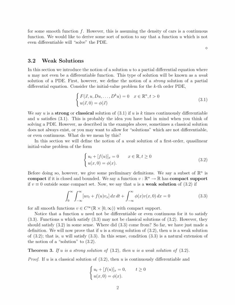
For t ≤ 1, our solution is defined as

u(x, t) =

1 x < t

1− x

1− tt < x < 1

0 x > 1.

(3.12)

However, notice that the curves intersect at t = 1. Beyond that time t, the different projectedcharacteristics are asking for our solution u to satisfy different conditions. This cannothappen. We no longer have a classical solution. Instead, let’s look for a weak solution of(3.10) for t ≥ 1 which satisfies (3.11).

From Theorem 4, a weak solution must satisfy the Rankine-Hugoniot jump conditiondiscussed above. That is, we need

[f(u)] = σ[u],

or more specifically,(u−)2

2− (u+)2

2= ξ′(t)[u− − u+].

Notice that the initial data for x < 0 wants u = 1, while the initial data for x > 1 wantsu = 0 for t ≥ 1. Let’s try to make a compromise by defining a curve x = ξ(t) such that u = 1to the left of the curve and u = 0 to the right of the curve. In other words, let u− = 1 andu+ = 0. Now our curve x = ξ(t) is defined for us by the Rankine-Hugoniot jump condition.In particular, we have

ξ′(t) =1

2.

In addition, we want our curve x = ξ(t) to contain the point (x, t) = (1, 1). Therefore, ourcurve must be given by (x− 1) = 1

2(t− 1) or x = t+1

2.

Therefore, for t ≥ 1, let

u(x, t) =

1 if x <t + 1

2

0 if x >t + 1

2.

(3.13)

Now u defined by (3.13) is a classical solution of (3.10) on either side of the curve x(t) =t+12

and u satisfies the Rankine-Hugoniot jump condition along the curve of discontinuity.Therefore, u(x, t) defined by (3.13) is a weak solution of (3.10) for t ≥ 1.

In summary, our solution of (3.10) with initial condition (3.11) is given by (3.12) fort ≤ 1 and (3.13) for t ≥ 1.

x

t

1

1u

uu

==

=0

1

11−−

xt

___

x= t 1+___2

7

Below we show a “movie” of our solution.

x

u

=0

1

1

x

u

=1/2

1

1

t t

x

u

t

1

1

x

u

=2

1

1

3/2

1 = t

¦Example 6. Consider Burger’s equation again,

ut + uux = 0 t ≥ 0

u(x, 0) = φ(x).(3.14)

But this time impose the initial condition,

φ(x) =

1 for x < 0

0 for x > 0.(3.15)

As before, u is constant along the projected characteristic curves given by x = φ(r)t + r. Ifr < 0, then φ(r) = 1 which implies the projected characteristic curves are x = t+ r for r < 0and the solution u should equal 1 along those curves. But, also, for r > 0, φ(r) = 0 whichmeans the projected characteristic curves are given by x = r for r > 0 and the solution ushould equal 0 along these curves.

8

x

t

1

1

Clearly, this is a contradiction and we can’t hope to find any continuous solution whichsolves this problem. Again, we look for a weak solution, by looking for a piecewise continu-ously differentiable function which satisfies the Rankine Hugoniot jump condition. We wantto find a curve x = ξ(t) such that u− = 1 to the left of the curve and u+ = 0 to the right ofthe curve. We need

[f(u)] = σ[u].

That is, we need(u−)2

2− (u+)2

2= ξ′(t)[u− − u+].

Substituting in for u− and u+, we get

ξ′(t) =1

2.

In addition, we want the curve x = ξ(t) to contain the point (x, t) = (0, 0). Therefore,our curve of discontinuity must be given by x = 1

2t. Therefore, our weak solution of (3.14)

satisfying (3.15) is given by

u(x, t) =

1 for x <t

2

0 for x >t

2.

x

t

1

1

x t= /2

u

u=

=

1

0

Below we show a “movie” of our solution.

9

x

u

=0

1

1

x

u

=1

1

1

1/2

t t

¦Example 7. We consider Burgers’ equation once again,

ut + uux = 0, t ≥ 0

u(x, 0) = φ(x)(3.16)

but now impose the initial condition

φ(x) =

0 for x < 0

1 for x > 0.(3.17)

Looking at our characteristics, we see that u should be constant along the projectedcharacteristic curves, x = φ(r)t + r. Here, if r < 0, then φ(r) = 0 and therefore, x = r.If r > 0, then φ(r) = 1 and therefore, x = t + r. Consequently, we have no crossing ofcharacteristics. However, we still have a problem. In fact, we have a region on which wedon’t have enough information! How should we define our solution in this region?

x

t

1

1

One Possibility. Let

u1(x, t) =

0 for x <t

2

1 for x >t

2.

Clearly, u1(x, t) is a classical solution on either side of the curve of discontinuity x = t2. In

addition, from the work of the previous example, it is easy to see that u1(x, t) satisfies theRankine-Hugoniot jump condition along the curve of discontinuity. Therefore, u1(x, t) is aweak solution of (3.16) satisfying (3.17). However, this is not the only possible solution.

10

x

t

1

1

x=t/2

u=0u=1

Another Possibility. Let

u2(x, t) =

0 for x ≤ 0x

tfor 0 ≤ x ≤ t

1 for x ≥ t.

Notice that u2(x, t) is a continuous solution of (3.16), (3.17). This type of solution which“fans” the wedge 0 < x < t is called a rarefaction wave.

x

t

1

1

u=0

u=1

u=x/t

We have found two different solutions. Is it possible, however, that one solution is morephysically realistic? If so, we would like to consider that our “real” solution. Below weintroduce the notion of an entropy condition. Solutions of quasilinear equations of the form(3.2) which satisfy this entropy condition are considered more physically realistic, and, thus,when looking for solutions of (3.2), we only allow for solutions which satisfy this extracondition. As we will see, solution u2(x, t) is considered to be the more physically realisticsolution and we consider that our “real” solution.

¦

3.3 Entropy Condition

Consider a quasilinear equation of the form

ut + [f(u)]x = 0.

11

This equation can also be written in the form

ut + f ′(u)ux = 0. (3.18)

The characteristic equations associated with (3.18) are given by

dx

ds= f ′(z)

dt

ds= 1

dz

ds= 0.

From these equations, we see that the speed of a solution u is given by

dx

dt= f ′(u).

In particular, for Burgers’ equation, the speed of a solution u is given by

dx

dt= u.

This says that taller waves move faster than shorter waves. In the case of Examples 5 and6, the initial wave was taller on the left, and, thus moving faster than the wave on the right.As a result, we expected the part of the wave to the left to overtake the part of the wave tothe right and cause the wave to break. This resulted in our curve of discontinuity.

In Example 7, however, for our initial data, the wave is higher to the right. Consequently,we expect the part of the wave to the right to move faster. Physically, therefore, we don’twant to allow for solution u1(x, t). Instead, we accept u2(x, t) as a physically more realisticsolution. See the movie of u2 below.

x

u

=0

1

1

x

u

=1

1

1

2 2

t t

Let’s make these ideas more precise. In particular, for an equation of the form (3.18), weonly allow for a curve of discontinuity in our solution u(x, t) if the wave to the left is movingfaster than the wave to the right. That is, we only allow for a curve of discontinuity betweenu− and u+ if

f ′(u−) > σ > f ′(u+). (3.19)

12

This is known as the entropy condition. We say that a curve of discontinuity is a shockcurve for a solution u if the curve satisfies the Rankine-Hugoniot jump condition and theentropy condition for that solution u. Therefore, to eliminate the physically less realisticsolutions, we only “accept” solutions u for which curves of discontinuity in the solution areshock curves. We state this more precisely as follows.

Consider the initial-value problem,

ut + [f(u)]x = 0 x ∈ R, t ≥ 0u(x, 0) = φ(x).

(3.20)

We say u is a weak, admissible solution of (3.20) only if u is a weak solution such that anycurve of discontinuity for u is a shock curve.

In Example 7, possibility one, for u− = 0, u+ = 1, σ = ξ′(t) = 12,

f ′(u−) = u− = 0 6> 1

26> 1 = u+ = f ′(u+).

Therefore, u1 does not satisfy the entropy condition along the curve of discontinuity x = t/2.Consequently, x = t/2 is not a shock curve, and, therefore, u1 is not an admissible solution.Solution u2, however, is a continuous solution. Therefore, we accept this solution as thephysically relevant one.

We now turn to initial-value problems of the form (3.20) when f has a particular structure.We say a function f is uniformly convex if there exists a constant θ > 0 such thatf ′′ ≥ θ > 0. In particular, this means f ′ is strictly increasing. If f ′ is strictly increasing,then u will satisfy the entropy condition (3.19) if and only if

u− > u+

on any curve of discontinuity. That is to say, for f uniformly convex, u will be a weak,admissible solution to

ut + [f(u)]x = 0,

if and only if u satisfies the Rankine-Hugoniot condition (3.9) and u satisfies

u− > u+

along any curves of discontinuity.

3.4 Riemann’s Problem

In this section, we study the initial value problem

ut + [f(u)]x = 0, t ≥ 0

u(x, 0) = φ(x)(3.21)

for the case when f is uniformly convex and the initial data is piecewise constant; that is,

φ(x) =

u− x < 0

u+ x > 0.(3.22)

The initial-value problem (3.21), (3.22) is known as Riemann’s Problem.

13

Theorem 8. (See Evans, Chap. 3) For f uniformly convex, there exists a unique weak,admissible* solution to Riemann’s problem (3.21), (3.22).

1. If u− > u+, then the admissible solution has a shock curve of speed σ and the solutionis given by

u(x, t) =

u−x

t< σ

u+ x

t> σ

(3.23)

where σ = [f(u)]/[u].

2. If u− < u+, then the solution has a rarefaction wave and the solution is given by

u(x, t) =

u−x

t< f ′(u−)

G(x/t) f ′(u−) <x

t< f ′(u+)

u+ x

t> f ′(u+),

(3.24)

where G ≡ (f ′)−1.

*Remark. For technical reasons, Evans presents a more precise definition of admissible toprove uniqueness. We will omit the proof of uniqueness here. See Evans.

Proof. First, let’s look at (1). Clearly, u(x, t) defined in (3.23) is a classical solution of (3.21),(3.22) on either side of the curve x = σt. In addition, the curve of discontinuity satisfies theRankine-Hugoniot jump condition (3.9), so u(x, t) is a weak solution. In addition, u− > u+

and f is uniformly convex. Therefore, u satisfies the entropy condition (3.19).Now, we look at (2). For u defined by (3.24), u is a classical solution of (3.21), (3.22) to

the left of x = f ′(u−)t and to the right of x = f ′(u+)t. Now we check that u is a solutionfor f ′(u−) < x/t < f ′(u+). By use of the chain rule, we have

ut + [f(u)]x = G′(x/t) · (−x/t2) + f ′(G(x/t)) · [G(x/t)]x

= G′(x/t) · (−x/t2) + f ′((f ′)−1(x/t)) ·G′(x/t) · (1/t)= G′(x/t) · (−x/t2) + G′(x/t) · (x/t2) = 0.

Therefore, we have shown that u is a classical solution in each of the three regions in whichit’s defined. Moreover, along the curve x/t = f ′(u−), G(x/t) = (f ′)−1(x/t) = u− impliesu(x, t) is continuous across the curve x/t = f ′(u−). Similarly, u(x, t) defined in (3.24) iscontinuous across the curve x/t = f ′(u+). Therefore, u has no curves of discontinuity andthus satisfies the entropy condition. It is easy to check that u satisfies (3.3), and, is thereforea weak solution of (3.21), (3.22).

Example 9. Consider the problem

ut + uux = 0, t ≥ 0

u(x, 0) = φ(x)

14

where

φ(x) =

1 0 < x < 1

0 otherwise.

The characteristic equations are given by

dt

ds= 1

dx

ds= z

dz

ds= 0

with initial conditions

t(r, 0) = 0

x(r, 0) = r

z(r, 0) = φ(r).

We know the solution is constant along the projected characteristic curves given by x(r, t) =φ(r)t + r.

If r < 0, then φ(r) = 0 implies x = r and u = 0 along these curves. If 0 < r < 1, thenφ(r) = 1 implies x = t + r and u = 1 along these curves. If r > 1, then φ(r) = 0 impliesx = r and u = 0 along these curves.

x

t

1

1

Therefore, we get a rarefaction wave between x = 0 and x = t and a shock is formed bythe intersection of the lines x = t + r for 0 < r < 1 and x = 1. By the Rankine-Hugoniotjump condition, the speed σ of the shock must satisfy

σ =[f(u)]

[u]

=(u−)2

2− (u+)2

2

u− − u+

=1/2− 0

1− 0=

1

2.

Therefore, the shock curve is given by x− 1 = 12t or x = 1 + t

2. So, our weak solution u will

take on the values shown below.

15

x

t

1

1

2

2

=0u

=1u

=0u

x t

x t

=

= /2+1u=x/t

Notice at t = 2, however, the rarefaction wave hits the shock curve x = 1 + t2. We need

the jump across the shock to satisfy the Rankine-Hugoniot jump condition. To the left ofthe jump, we have u− = x/t and to the right, we have u+ = 0. The Rankine-Hugoniot jumpcondition becomes

σ =[f(u)]

[u]

=(u−)2

2− (u+)2

2

u− − u+

=12

(xt

)2 − 0xt− 0

=x

2t.

Therefore, we get a new shock curve emanating from the point (2, 2) with speed σ = ξ′(t) =x/2t. This curve is given by x(t) =

√2t. Therefore the weak solution u will take on the

values shown below.

x

t

1

2

=0u

=1u

=0u

x t

x t

=

= /2+1u=x/t

1 2

=(2 )x t1/2

16

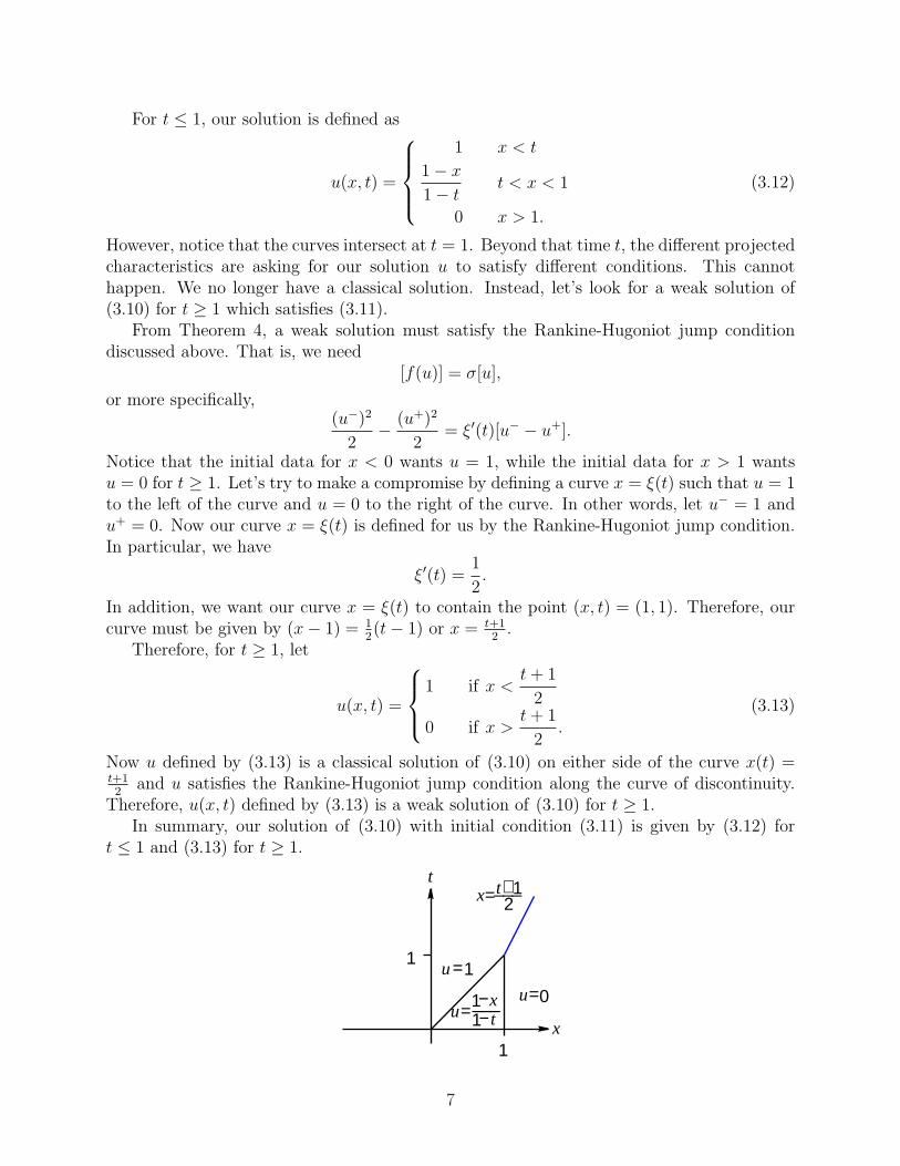
To summarize, we have

u(x, t) =

0 for x < 0

x/t for 0 < x < t

1 for t < x < 1 +t

2

0 for x > 1 +t

2

for t ≤ 2, and

u(x, t) =

0 if x < 0

x/t if 0 < x <√

2t

0 if√

2t < x

for t ≥ 2.

x

u

=0

1

1

x

u

=1

1

1

t t

3/2

x

u

=2

1

1

x

u

=9/2

1

1

t t

2 2 3

2/3

¦

3.5 Long-Time Asymptotics

Notice in Example 9 that |u| → 0 as t → +∞. In fact, by using the solution formula, we seethat for 0 ≤ t ≤ 2, |u(x, t)| ≤ 1 and for t ≥ 2,

|u(x, t)| ≤ x

t≤√

2t

t=

√2√t.

17

In summary, we have

|u(x, t)| ≤√

2√t

for all t > 0, all x ∈ R. Thus, u decays to zero like 1/√

t as t → +∞. This property is truein general for solutions of the initial-value problem

ut + [f(u)]x = 0, t ≥ 0

u(x, 0) = φ(x)(3.25)

assuming

1. φ(x) is bounded and integrable

2. f is smooth, uniformly convex and f(0) = 0.

We state this more precisely in the following theorem.

Theorem 10. (See Evans, Chapter 3) Consider an initial-value problem of the form (3.25)where φ and f satisfy the hypothesis indicated. Then the solution u of (3.25) satisfies thefollowing decay estimate. There exists a constant C > 0 such that

|u(x, t)| ≤ C√t

for all t > 0, all x ∈ R.

Proof. See Evans.

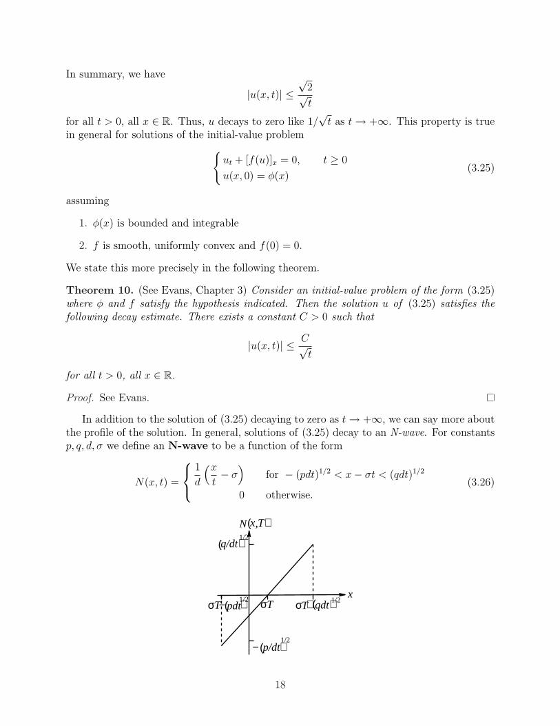
In addition to the solution of (3.25) decaying to zero as t → +∞, we can say more aboutthe profile of the solution. In general, solutions of (3.25) decay to an N-wave. For constantsp, q, d, σ we define an N-wave to be a function of the form

N(x, t) =

1

d

(x

t− σ

)for − (pdt)1/2 < x− σt < (qdt)1/2

0 otherwise.(3.26)

x

N( )Tx,

σT σT+ qdt( )1/2

q/dt(1/2)

σT− pdt( )1/2

p/dt( )−1/2

18

We now define a specific N-wave using the constants defined below. Let p, q, d and σ bedefined as follows. Let

p = −2 miny∈R

∫ y

−∞φ(x) dx

q = 2 maxy∈R

∫ ∞

y

φ(x) dx

d = f ′′(0)

σ = f ′(0).

(3.27)

Theorem 11. (See Evans, Chapter 3) For an initial-value problem of the form (3.25) wheref is smooth and uniformly convex and φ has compact support, then for p, q, d, σ definedin (3.27) and N(x, t) defined in (3.26) for this choice of constants p, q, d, σ, there exists aconstant C > 0 such that the solution u of (3.25) satisfies

∫ ∞

−∞|u(x, t)−N(x, t)| dx ≤ C√

t

for all t > 0.

Proof. See Evans.

Example 12. For Example 9, p = 0, q = 2, f(u) = u2/2 implies σ = f ′(0) = 0 andd = f ′′(0) = 1. Therefore,

N(x, t) =

x/t for 0 < x <

√2t

0 otherwise,

and Theorem 11 says there exists a constant C > 0 such that

∫ ∞

−∞|u(x, t)−N(x, t)| dx ≤ C√

t.

We see that this statement is true because for 0 ≤ t ≤ 2,

∫ ∞

−∞|u(x, t)−N(x, t)| dx =

∫ 1+t/2

0

|u(x, t)−N(x, t)| dx

=

∫ t

0

|x/t− x/t| dx +

∫ √2t

t

|1− x/t| dx +

∫ 1+t/2

√2t

|1− 0| dx

≤ (1 +√

2t/t)[√

2t− t] + [1 + t/2−√

2t]

= 3− t

2−√

2t ≤ 6√

2√t

,

while u(x, t) = N(x, t) for t ≥ 2. ¦

19

3.6 Oleinik Entropy Condition.

In this section, we consider quasilinear first-order initial-value problems in the case when fis not uniformly convex.

Recall for an equation of the form

ut + [f(u)]x = 0, (3.28)

f ′(u) is the speed of the wave with height u. Recall the entropy condition

f ′(u−) > σ > f ′(u+) (3.29)

where σ = [f(u)]/[u]. For the case when f is uniformly convex, requiring that curves ofdiscontinuity satisfy the entropy condition (3.29) guarantees uniqueness of solutions. In thecase, when f is not uniformly convex, condition (3.29) is not enough to guarantee uniquenessof solutions.

First, we make some remarks on the entropy condition. In general, we only want to allowfor a curve of discontinuity x = ξ(t) if the speed of the wave to the left of the curve is greaterthan or equal to the speed σ = ξ′(t) of the curve of discontinuity, and σ is greater than orequal to the speed of the wave to the right of the curve of discontinuity. If f is uniformlyconvex, meaning f ′ is strictly increasing, then for u− 6= u+, there are two possibilities:

1. f ′(u−) > σ > f ′(u+)

2. f ′(u−) < σ < f ′(u+).

Therefore, for f uniformly convex, we only want to allow for a curve of discontinuity in thecase when

f ′(u−) > σ > f ′(u+).

Consequently, we take this as our entropy condition.More generally, for f not necessarily uniformly convex, we only want to allow for a curve

of discontinuity x = ξ(t) in the case when

f ′(u−) ≥ σ ≥ f ′(u+).

As shown in the following example, however, this condition is not enough to guaranteeuniqueness of solutions.

Example 13. Consider the initial-value problem

ut + [f(u)]x = 0, t ≥ 0

u(x, 0) = φ(x)

where

φ(x) =

u− x < 0

u+ x > 0

for f, u−, u+ shown below.

20

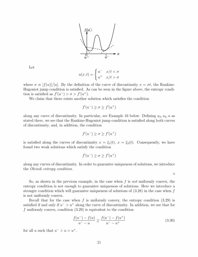
uuu

f (u)

+ −

Let

u(x, t) =

u− x/t < σ

u+ x/t > σ

where σ ≡ [f(u)]/[u]. By the definition of the curve of discontinuity x = σt, the Rankine-Hugoniot jump condition is satisfied. As can be seen in the figure above, the entropy condi-tion is satisfied as f ′(u−) > σ > f ′(u+).

We claim that there exists another solution which satisfies the condition

f ′(u−) ≥ σ ≥ f ′(u+)

along any curve of discontinuity. In particular, see Example 16 below. Defining u2, u3, u asstated there, we see that the Rankine-Hugoniot jump condition is satisfied along both curvesof discontinuity, and, in addition, the condition

f ′(u−) ≥ σ ≥ f ′(u+)

is satisfied along the curves of discontinuity x = ξ1(t), x = ξ2(t). Consequently, we havefound two weak solutions which satisfy the condition

f ′(u−) ≥ σ ≥ f ′(u+)

along any curves of discontinuity. In order to guarantee uniqueness of solutions, we introducethe Oleinik entropy condition.

¦So, as shown in the previous example, in the case when f is not uniformly convex, the

entropy condition is not enough to guarantee uniqueness of solutions. Here we introduce astronger condition which will guarantee uniqueness of solutions of (3.28) in the case when fis not uniformly convex.

Recall that for the case when f is uniformly convex, the entropy condition (3.29) issatisfied if and only if u− > u+ along the curve of discontinuity. In addition, we see that forf uniformly convex, condition (3.29) is equivalent to the condition

f(u−)− f(u)

u− − u≥ f(u−)− f(u+)

u− − u+(3.30)

for all u such that u− > u > u+.

21

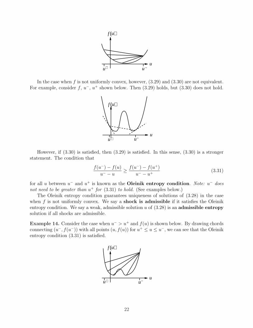
uuu

f (u)

+ −

In the case when f is not uniformly convex, however, (3.29) and (3.30) are not equivalent.For example, consider f , u−, u+ shown below. Then (3.29) holds, but (3.30) does not hold.

uuu

f (u)

+ −

However, if (3.30) is satisfied, then (3.29) is satisfied. In this sense, (3.30) is a strongerstatement. The condition that

f(u−)− f(u)

u− − u≥ f(u−)− f(u+)

u− − u+(3.31)

for all u between u− and u+ is known as the Oleinik entropy condition. Note: u− doesnot need to be greater than u+ for (3.31) to hold. (See examples below.)

The Oleinik entropy condition guarantees uniqueness of solutions of (3.28) in the casewhen f is not uniformly convex. We say a shock is admissible if it satisfies the Oleinikentropy condition. We say a weak, admissible solution u of (3.28) is an admissible entropysolution if all shocks are admissible.

Example 14. Consider the case when u− > u+ and f(u) is shown below. By drawing chordsconnecting (u−, f(u−)) with all points (u, f(u)) for u+ ≤ u ≤ u−, we can see that the Oleinikentropy condition (3.31) is satisfied.

uuu

f (u)

+ −

22

Therefore, for the initial-value problem

ut + [f(u)]x = 0, t ≥ 0

u(x, 0) = φ(x)

where

φ(x) =

u− for x < 0

u+ for x > 0

with f(u) as shown above, a shock is admissible, and the solution is given by

u(x, t) =

u− for x/t < σ

u+ for x/t > σ

where as usual σ = [f(u)]/[u].

x

tx t=

u

u=

= u

u

σ−

+

¦Example 15. Now consider the case when u+ > u− and f(u) is as shown below. Again,by drawing chords connecting (u−, f(u−)) and (u, f(u)) for all u between u− and u+, we seethat the Oleinik entropy condition is satisfied.

uuu

f (u)

+−

Therefore, a shock is admissible and the solution of the initial-value problem

ut + [f(u)]x = 0, t ≥ 0

u(x, 0) = φ(x)

where

φ(x) =

u− for x < 0

u+ for x > 0

23

with f(u) as shown above is given by

u(x, t) =

u− for x/t < σ

u+ for x/t > σ.

¦To summarize, we have shown the following. If either of the following hold:

1. u− > u+ and the chord connecting (u−, f(u−)) and (u+, f(u+)) lies above the graph off(u)

2. u+ > u− and the chord connecting (u−, f(u−)) and (u−, f(u+)) lies below the graph off(u),

then a shock is admissible and the solution ofut + [f(u)]x = 0, t ≥ 0

u(x, 0) = φ(x)

where

φ(x) =

u− for x < 0

u+ for x > 0,

is given by

u(x, t) =

u− for x/t < σ

u+ for x/t > σ

where σ = [f(u)]/[u] is defined by the Rankine-Hugoniot jump condition (3.9).

Now what happens if u−, u+ and f are such that neither of the conditions above hold?We will get a combination of rarefaction waves and shock curves.

Example 16. Consider the initial-value problem

ut + [f(u)]x = 0, t ≥ 0

u(x, 0) = φ(x)(3.32)

where

φ(x) =

u− for x < 0

u+ for x > 0(3.33)

with f , u− and u+ as shown in the picture below.

uuu

f (u)

+ −

24

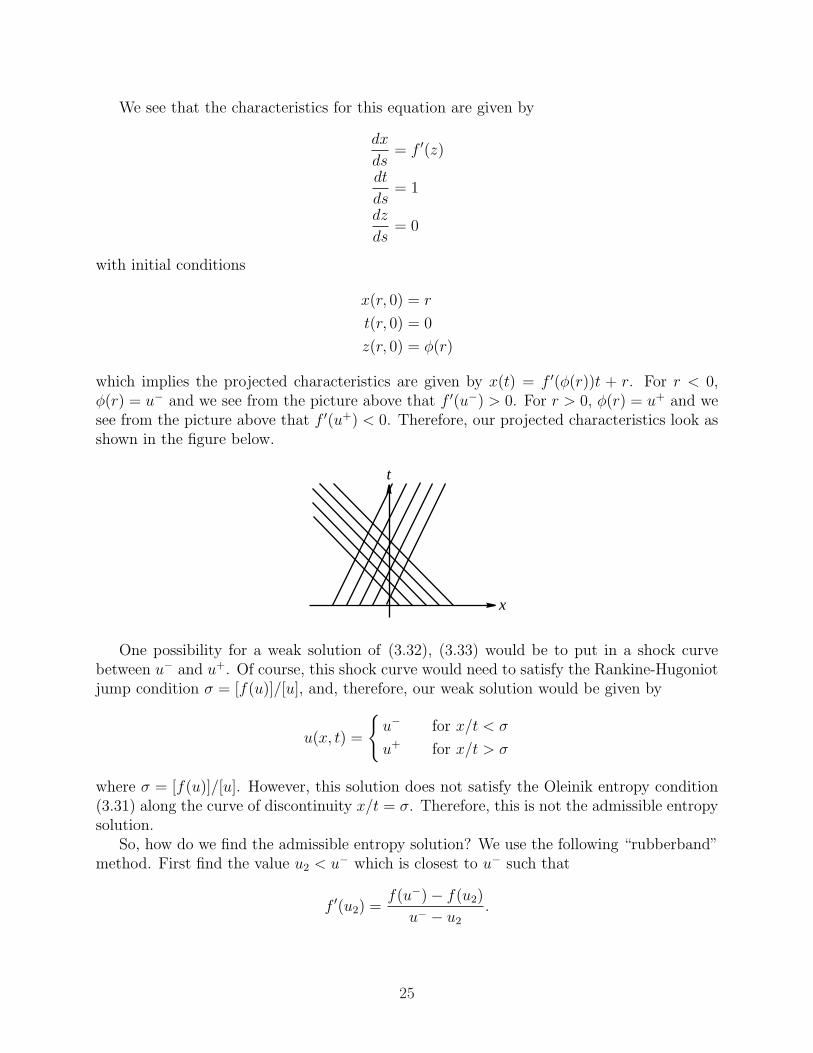
We see that the characteristics for this equation are given by

dx

ds= f ′(z)

dt

ds= 1

dz

ds= 0

with initial conditions

x(r, 0) = r

t(r, 0) = 0

z(r, 0) = φ(r)

which implies the projected characteristics are given by x(t) = f ′(φ(r))t + r. For r < 0,φ(r) = u− and we see from the picture above that f ′(u−) > 0. For r > 0, φ(r) = u+ and wesee from the picture above that f ′(u+) < 0. Therefore, our projected characteristics look asshown in the figure below.

x

t

One possibility for a weak solution of (3.32), (3.33) would be to put in a shock curvebetween u− and u+. Of course, this shock curve would need to satisfy the Rankine-Hugoniotjump condition σ = [f(u)]/[u], and, therefore, our weak solution would be given by

u(x, t) =

u− for x/t < σ

u+ for x/t > σ

where σ = [f(u)]/[u]. However, this solution does not satisfy the Oleinik entropy condition(3.31) along the curve of discontinuity x/t = σ. Therefore, this is not the admissible entropysolution.

So, how do we find the admissible entropy solution? We use the following “rubberband”method. First find the value u2 < u− which is closest to u− such that

f ′(u2) =f(u−)− f(u2)

u− − u2

.

25

uuu

f (u)

+ −uu 23

Then for u2 < u < u−,f(u−)− f(u)

u− − u≥ f(u−)− f(u2)

u− − u2

.

Therefore, u−, u2 satisfy the Oleinik entropy condition, so we can put in a shock curve,x = ξ1(t) from u− to u2. This shock curve must satisfy the Rankine-Hugoniot jump condition(3.9). Therefore,

ξ′1(t) =f(u−)− f(u2)

u− − u2

= f ′(u2).

Next, find u3 such that

f ′(u3) =f(u3)− f(u+)

u3 − u+.

Therefore,f(u3)− f(u)

u3 − u≥ f(u3)− f(u+)

u3 − u+

for all u between u+ and u3, so u3, u+ satisfy the Oleinik entropy condition and we can put

in a shock curve x = ξ2(t) between u3 and u+. This shock curve will satisfy

ξ′2(t) =f(u3)− f(u+)

u3 − u+= f ′(u3).

Then between these shock curves, we put in a rarefaction wave from u2 to u3. Therefore,our solution is given by

u(x, t) =

u− for x/t < f ′(u2)

G(x/t) for f ′(u2) < x/t < f ′(u3)

u+ for f ′(u3) < x/t

where G = (f ′)−1.

x

t

x t=

u

u=

= u

u−

+x ξ= (t)

ξ( )

1

2

u= ( )x tG /

26

¦For further information on the Oleinik entropy condition and weak solutions of the initial-

value problem ut + [f(u)]x = 0, t ≥ 0

u(x, 0) = φ(x)

in the case when f does not have any convexity assumptions, see the following reference.

Reference: D. Ballou, Solutions to Nonlinear Hyperbolic Cauchy Problems without Con-vexity Conditions, Transactions of the American Mathematical Society, 152, Dec. 1970,441-460.

27