3 Basic Properties of Matrices

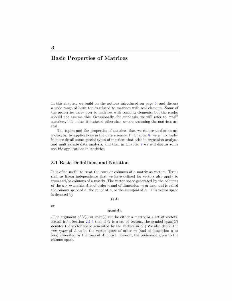
3

Basic Properties of Matrices

In this chapter, we build on the notions introduced on page 5, and discussa wide range of basic topics related to matrices with real elements. Some ofthe properties carry over to matrices with complex elements, but the readershould not assume this. Occasionally, for emphasis, we will refer to “real”matrices, but unless it is stated otherwise, we are assuming the matrices arereal.

The topics and the properties of matrices that we choose to discuss aremotivated by applications in the data sciences. In Chapter 8, we will considerin more detail some special types of matrices that arise in regression analysisand multivariate data analysis, and then in Chapter 9 we will discuss somespecific applications in statistics.

3.1 Basic Definitions and Notation

It is often useful to treat the rows or columns of a matrix as vectors. Termssuch as linear independence that we have defined for vectors also apply torows and/or columns of a matrix. The vector space generated by the columnsof the n×m matrix A is of order n and of dimension m or less, and is calledthe column space of A, the range of A, or the manifold of A. This vector spaceis denoted by

V(A)

orspan(A).

(The argument of V(·) or span(·) can be either a matrix or a set of vectors.Recall from Section 2.1.3 that if G is a set of vectors, the symbol span(G)denotes the vector space generated by the vectors in G.) We also define therow space of A to be the vector space of order m (and of dimension n orless) generated by the rows of A; notice, however, the preference given to thecolumn space.

52 3 Basic Properties of Matrices

Many of the properties of matrices that we discuss hold for matrices withan infinite number of elements, but throughout this book we will assume thatthe matrices have a finite number of elements, and hence the vector spacesare of finite order and have a finite number of dimensions.

Similar to our definition of multiplication of a vector by a scalar, we definethe multiplication of a matrix A by a scalar c as

cA = (caij).

The aii elements of a matrix are called diagonal elements; an elementaij with i < j is said to be “above the diagonal”, and one with i > j issaid to be “below the diagonal”. The vector consisting of all of the aii’s iscalled the principal diagonal or just the diagonal. The elements ai,i+ck

arecalled “codiagonals” or “minor diagonals”. If the matrix has m columns, theai,m+1−i elements of the matrix are called skew diagonal elements. We useterms similar to those for diagonal elements for elements above and belowthe skew diagonal elements. These phrases are used with both square andnonsquare matrices. The diagonal begins in the first row and first column(that is, a11), and ends at akk, where k is the minimum of the number of rowsand the number of columns.

If, in the matrix A with elements aij for all i and j, aij = aji, A is saidto be symmetric. A symmetric matrix is necessarily square. A matrix A suchthat aij = −aji is said to be skew symmetric. The diagonal entries of a skewsymmetric matrix must be 0. If aij = aji (where a represents the conjugateof the complex number a), A is said to be Hermitian. A Hermitian matrix isalso necessarily square, and, of course, a real symmetric matrix is Hermitian.A Hermitian matrix is also called a self-adjoint matrix.

Diagonal, Hollow, and Diagonally Dominant Matrices

If all except the principal diagonal elements of a matrix are 0, the matrix iscalled a diagonal matrix. A diagonal matrix is the most common and mostimportant type of sparse matrix. If all of the principal diagonal elements of amatrix are 0, the matrix is called a hollow matrix. A skew symmetric matrixis hollow, for example. If all except the principal skew diagonal elements of amatrix are 0, the matrix is called a skew diagonal matrix.

An n×m matrix A for which

|aii| >m∑

j 6=i

|aij| for each i = 1, . . . , n (3.1)

is said to be row diagonally dominant; one for which |ajj| >∑n

i 6=j |aij| for eachj = 1, . . . , m is said to be column diagonally dominant. (Some authors referto this as strict diagonal dominance and use “diagonal dominance” withoutqualification to allow the possibility that the inequalities in the definitions

3.1 Basic Definitions and Notation 53

are not strict.) Most interesting properties of such matrices hold whether thedominance is by row or by column. If A is symmetric, row and column di-agonal dominances are equivalent, so we refer to row or column diagonallydominant symmetric matrices without the qualification; that is, as just diag-onally dominant.

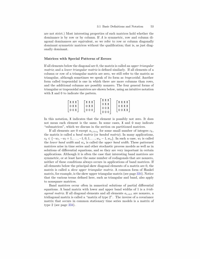
Matrices with Special Patterns of Zeroes

If all elements below the diagonal are 0, the matrix is called an upper triangularmatrix; and a lower triangular matrix is defined similarly. If all elements of acolumn or row of a triangular matrix are zero, we still refer to the matrix astriangular, although sometimes we speak of its form as trapezoidal. Anotherform called trapezoidal is one in which there are more columns than rows,and the additional columns are possibly nonzero. The four general forms oftriangular or trapezoidal matrices are shown below, using an intuitive notationwith X and 0 to indicate the pattern.

X X X

0 X X

0 0 X

X X X

0 X X

0 0 0

X X X

0 X X

0 0 X

0 0 0

X X X X

0 X X X

0 0 X X

In this notation, X indicates that the element is possibly not zero. It doesnot mean each element is the same. In some cases, X and 0 may indicate“submatrices”, which we discuss in the section on partitioned matrices.

If all elements are 0 except ai,i+ckfor some small number of integers ck,

the matrix is called a band matrix (or banded matrix). In many applications,ck ∈ {−wl,−wl + 1, . . . ,−1, 0, 1, . . . , wu − 1, wu}. In such a case, wl is calledthe lower band width and wu is called the upper band width. These patternedmatrices arise in time series and other stochastic process models as well as insolutions of differential equations, and so they are very important in certainapplications. Although it is often the case that interesting band matrices aresymmetric, or at least have the same number of codiagonals that are nonzero,neither of these conditions always occurs in applications of band matrices. Ifall elements below the principal skew diagonal elements of a matrix are 0, thematrix is called a skew upper triangular matrix. A common form of Hankelmatrix, for example, is the skew upper triangular matrix (see page 334). Noticethat the various terms defined here, such as triangular and band, also applyto nonsquare matrices.

Band matrices occur often in numerical solutions of partial differentialequations. A band matrix with lower and upper band widths of 1 is a tridi-agonal matrix. If all diagonal elements and all elements ai,i±1 are nonzero, atridiagonal matrix is called a “matrix of type 2”. The inverse of a covariancematrix that occurs in common stationary time series models is a matrix oftype 2 (see page 334).


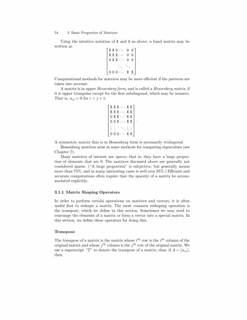
Using the intuitive notation of X and 0 as above, a band matrix may bewritten as

X X 0 · · · 0 0

X X X · · · 0 0

0 X X · · · 0 0

. . .. . .

0 0 0 · · · X X

.

Computational methods for matrices may be more efficient if the patterns aretaken into account.

A matrix is in upper Hessenberg form, and is called a Hessenberg matrix, ifit is upper triangular except for the first subdiagonal, which may be nonzero.That is, aij = 0 for i > j + 1:

X X X · · · X X

X X X · · · X X

0 X X · · · X X

0 0 X · · · X X...

.... . .

......

0 0 0 · · · X X

.

A symmetric matrix that is in Hessenberg form is necessarily tridiagonal.Hessenberg matrices arise in some methods for computing eigenvalues (see

Chapter 7).Many matrices of interest are sparse; that is, they have a large propor-

tion of elements that are 0. The matrices discussed above are generally notconsidered sparse. (“A large proportion” is subjective, but generally meansmore than 75%, and in many interesting cases is well over 95%.) Efficient andaccurate computations often require that the sparsity of a matrix be accom-modated explicitly.

3.1.1 Matrix Shaping Operators

In order to perform certain operations on matrices and vectors, it is oftenuseful first to reshape a matrix. The most common reshaping operation isthe transpose, which we define in this section. Sometimes we may need torearrange the elements of a matrix or form a vector into a special matrix. Inthis section, we define three operators for doing this.

Transpose

The transpose of a matrix is the matrix whose ith row is the ith column of theoriginal matrix and whose jth column is the jth row of the original matrix. Weuse a superscript “T” to denote the transpose of a matrix; thus, if A = (aij),then


AT = (aji). (3.2)

(In other literature, the transpose is often denoted by a prime, as in A′ =(aji) = AT.)

If the elements of the matrix are from the field of complex numbers, theconjugate transpose, also called the adjoint, is more useful than the transpose.(“Adjoint” is also used to denote another type of matrix, so we will generallyavoid using that term. This meaning of the word is the origin of the otherterm for a Hermitian matrix, a “self-adjoint matrix”.) We use a superscript“H” to denote the conjugate transpose of a matrix; thus, if A = (aij), thenAH = (aji). We also use a similar notation for vectors. If the elements of Aare all real, then AH = AT. (The conjugate transpose is often denoted by anasterisk, as in A∗ = (aji) = AH. This notation is more common if a prime isused to denote the transpose. We sometimes use the notation A∗ to denote ag2 inverse of the matrix A; see page 117.)

If (and only if) A is symmetric, A = AT; if (and only if) A is skew sym-metric, AT = −A; and if (and only if) A is Hermitian, A = AH.

Diagonal Matrices and Diagonal Vectors: diag(·) and vecdiag(·)

A square diagonal matrix can be specified by the diag(·) constructor functionthat operates on a vector and forms a diagonal matrix with the elements ofthe vector along the diagonal:

diag((d1, d2, . . . , dn)

)=

d1 0 · · · 00 d2 · · · 0

. . .

0 0 · · · dn

. (3.3)

(Notice that the argument of diag is a vector; that is why there are two setsof parentheses in the expression above, although sometimes we omit one setwithout loss of clarity.) The diag function defined here is a mapping IRn 7→IRn×n. Later we will extend this definition slightly.

A very important diagonal matrix has all 1s along the diagonal. If it hasn diagonal elements, it is denoted by In; so In = diag(1n). This is called theidentity matrix of order n. The size is often omitted, and we call it the identitymatrix, and denote it by I.

The vecdiag(·) function forms a vector from the principal diagonal elementsof a matrix. If A is an n×m matrix, and k = min(n, m),

vecdiag(A) = (a11, . . . , akk). (3.4)

The vecdiag function defined here is a mapping IRn×m 7→ IRmin(n,m).Sometimes we overload diag(·) to allow its argument to be a matrix, and

in that case, it is the same as vecdiag(·). Both the R and Matlab computingsystems, for example, use this overloading; that is, they each provide a singlefunction (called diag in each case).


Forming a Vector from the Elements of a Matrix: vec(·) andvech(·)

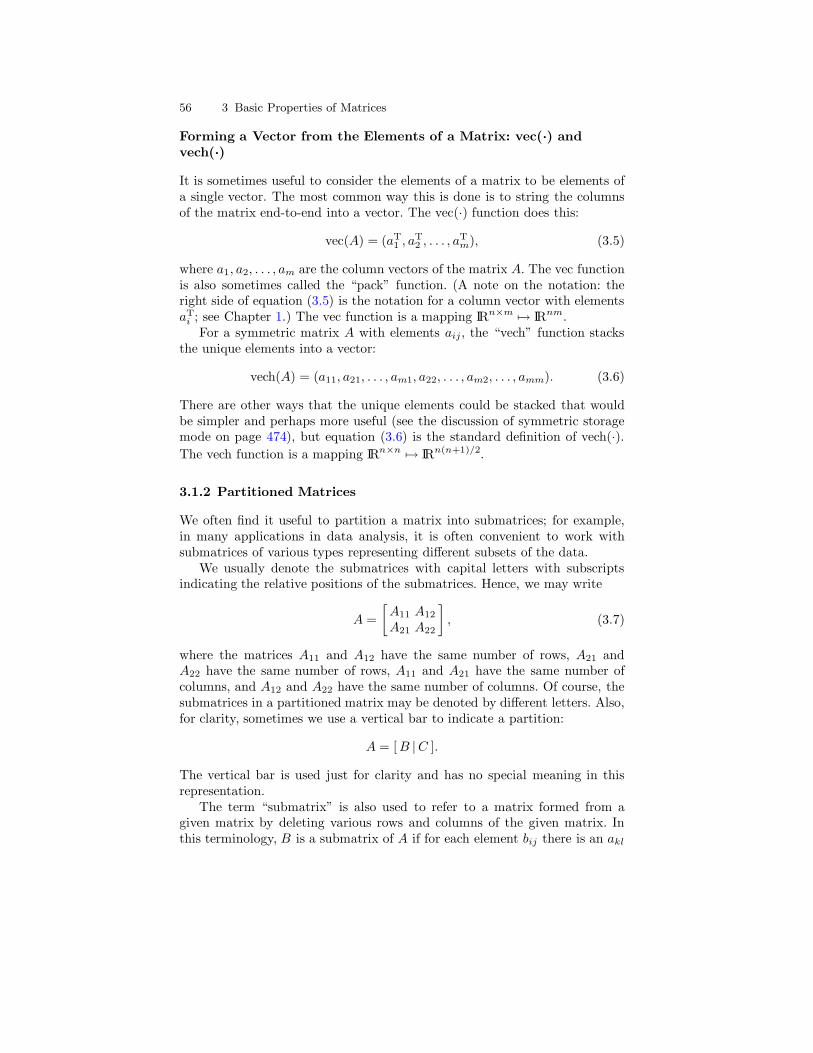
It is sometimes useful to consider the elements of a matrix to be elements ofa single vector. The most common way this is done is to string the columnsof the matrix end-to-end into a vector. The vec(·) function does this:

vec(A) = (aT1 , aT

2 , . . . , aTm), (3.5)

where a1, a2, . . . , am are the column vectors of the matrix A. The vec functionis also sometimes called the “pack” function. (A note on the notation: theright side of equation (3.5) is the notation for a column vector with elementsaT

i ; see Chapter 1.) The vec function is a mapping IRn×m 7→ IRnm.For a symmetric matrix A with elements aij, the “vech” function stacks

the unique elements into a vector:

vech(A) = (a11, a21, . . . , am1, a22, . . . , am2, . . . , amm). (3.6)

There are other ways that the unique elements could be stacked that wouldbe simpler and perhaps more useful (see the discussion of symmetric storagemode on page 474), but equation (3.6) is the standard definition of vech(·).The vech function is a mapping IRn×n 7→ IRn(n+1)/2.

3.1.2 Partitioned Matrices

We often find it useful to partition a matrix into submatrices; for example,in many applications in data analysis, it is often convenient to work withsubmatrices of various types representing different subsets of the data.

We usually denote the submatrices with capital letters with subscriptsindicating the relative positions of the submatrices. Hence, we may write

A =

[A11 A12

A21 A22

], (3.7)

where the matrices A11 and A12 have the same number of rows, A21 andA22 have the same number of rows, A11 and A21 have the same number ofcolumns, and A12 and A22 have the same number of columns. Of course, thesubmatrices in a partitioned matrix may be denoted by different letters. Also,for clarity, sometimes we use a vertical bar to indicate a partition:

A = [ B |C ].

The vertical bar is used just for clarity and has no special meaning in thisrepresentation.

The term “submatrix” is also used to refer to a matrix formed from agiven matrix by deleting various rows and columns of the given matrix. Inthis terminology, B is a submatrix of A if for each element bij there is an akl


with k ≥ i and l ≥ j such that bij = akl; that is, the rows and/or columns ofthe submatrix are not necessarily contiguous in the original matrix. This kindof subsetting is often done in data analysis, for example, in variable selectionin linear regression analysis.

A square submatrix whose principal diagonal elements are elements of theprincipal diagonal of the given matrix is called a principal submatrix. If A11 inthe example above is square, it is a principal submatrix, and if A22 is square,it is also a principal submatrix. Sometimes the term “principal submatrix” isrestricted to square submatrices. If a matrix is diagonally dominant, then itis clear that any principal submatrix of it is also diagonally dominant.

A principal submatrix that contains the (1, 1) element and whose rowsand columns are contiguous in the original matrix is called a leading principalsubmatrix. If A11 is square, it is a leading principal submatrix in the exampleabove.

Partitioned matrices may have useful patterns. A “block diagonal” matrixis one of the form

X 0 · · · 00 X · · · 0

. . .

0 0 · · · X

,

where 0 represents a submatrix with all zeros and X represents a generalsubmatrix with at least some nonzeros.

The diag(·) function previously introduced for a vector is also defined fora list of matrices:

diag(A1, A2, . . . , Ak)

denotes the block diagonal matrix with submatrices A1, A2, . . . , Ak along thediagonal and zeros elsewhere. A matrix formed in this way is sometimes calleda direct sum of A1, A2, . . . , Ak, and the operation is denoted by ⊕:

A1 ⊕ · · · ⊕Ak = diag(A1, . . . , Ak). (3.8)

Although the direct sum is a binary operation, we are justified in definingit for a list of matrices because the operation is clearly associative.

The Ai may be of different sizes and they may not be square, although inmost applications the matrices are square (and some authors define the directsum only for square matrices).

We will define vector spaces of matrices below and then recall the definitionof a direct sum of vector spaces (page 18), which is different from the directsum defined above in terms of diag(·).

Transposes of Partitioned Matrices

The transpose of a partitioned matrix is formed in the obvious way; for ex-ample,


[A11 A12 A13

A21 A22 A23

]T=

AT

11 AT21

AT12 AT

22

AT13 AT

23

. (3.9)

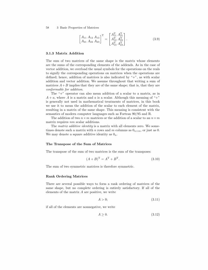
3.1.3 Matrix Addition

The sum of two matrices of the same shape is the matrix whose elementsare the sums of the corresponding elements of the addends. As in the case ofvector addition, we overload the usual symbols for the operations on the realsto signify the corresponding operations on matrices when the operations aredefined; hence, addition of matrices is also indicated by “+”, as with scalaraddition and vector addition. We assume throughout that writing a sum ofmatrices A+B implies that they are of the same shape; that is, that they areconformable for addition.

The “+” operator can also mean addition of a scalar to a matrix, as inA + a, where A is a matrix and a is a scalar. Although this meaning of “+”is generally not used in mathematical treatments of matrices, in this bookwe use it to mean the addition of the scalar to each element of the matrix,resulting in a matrix of the same shape. This meaning is consistent with thesemantics of modern computer languages such as Fortran 90/95 and R.

The addition of two n×m matrices or the addition of a scalar to an n×mmatrix requires nm scalar additions.

The matrix additive identity is a matrix with all elements zero. We some-times denote such a matrix with n rows and m columns as 0n×m, or just as 0.We may denote a square additive identity as 0n.

The Transpose of the Sum of Matrices

The transpose of the sum of two matrices is the sum of the transposes:

(A + B)T = AT + BT. (3.10)

The sum of two symmetric matrices is therefore symmetric.

Rank Ordering Matrices

There are several possible ways to form a rank ordering of matrices of thesame shape, but no complete ordering is entirely satisfactory. If all of theelements of the matrix A are positive, we write

A > 0; (3.11)

if all of the elements are nonnegative, we write

A ≥ 0. (3.12)


The terms “positive” and “nonnegative” and these symbols are not to beconfused with the terms “positive definite” and “nonnegative definite” andsimilar symbols for important classes of matrices having different properties(which we will introduce in equation (3.66) and discuss further in Section 8.3.)

Vector Spaces of Matrices

Having defined scalar multiplication and matrix addition (for conformablematrices), we can define a vector space of n ×m matrices as any set that isclosed with respect to those operations. The individual operations of scalarmultiplication and matrix addition allow us to define an axpy operation onthe matrices, as in equation (2.1) on page 12. Closure of this space impliesthat it must contain the additive identity, just as we saw on page 13). Thematrix additive identity is the 0 matrix.

As with any vector space, we have the concepts of linear independence,generating set or spanning set, basis set, essentially disjoint spaces, and directsums of matrix vector spaces (as in equation (2.10), which is different fromthe direct sum of matrices defined in terms of diag(·) as in equation (3.8)).

An important vector space of matrices is IRn×m. For matrices X, Y ∈IRn×m and a ∈ IR, the axpy operation is aX + Y .

If n ≥ m, a set of nm n×m matrices whose columns consist of all combina-tions of a set of n n-vectors that span IRn is a basis set for IRn×m. If n < m,we can likewise form a basis set for IRn×m or for subspaces of IRn×m in asimilar way. If {B1, . . . , Bk} is a basis set for IRn×m, then any n ×m matrix

can be represented as∑k

i=1 ciBi. Subsets of a basis set generate subspaces ofIRn×m.

Because the sum of two symmetric matrices is symmetric, and a scalarmultiple of a symmetric matrix is likewise symmetric, we have a vector spaceof the n × n symmetric matrices. This is clearly a subspace of the vectorspace IRn×n. All vectors in any basis for this vector space must be symmetric.Using a process similar to our development of a basis for a general vectorspace of matrices, we see that there are n(n + 1)/2 matrices in the basis (seeExercise 3.1).

3.1.4 Scalar-Valued Operators on Square Matrices:The Trace

There are several useful mappings from matrices to real numbers; that is, fromIRn×m to IR. Some important ones are norms, which are similar to vectornorms and which we will consider later. In this section and the next, wedefine two scalar-valued operators, the trace and the determinant, that applyto square matrices.


The Trace: tr(·)

The sum of the diagonal elements of a square matrix is called the trace of thematrix. We use the notation “tr(A)” to denote the trace of the matrix A:

tr(A) =∑

i

aii. (3.13)

The Trace of the Transpose of Square Matrices

From the definition, we see

tr(A) = tr(AT). (3.14)

The Trace of Scalar Products of Square Matrices

For a scalar c and an n× n matrix A,

tr(cA) = c tr(A).

This follows immediately from the definition because for tr(cA) each diagonalelement is multiplied by c.

The Trace of Partitioned Square Matrices

If the square matrix A is partitioned such that the diagonal blocks are squaresubmatrices, that is,

A =

[A11 A12

A21 A22

], (3.15)

where A11 and A22 are square, then from the definition, we see that

tr(A) = tr(A11) + tr(A22). (3.16)

The Trace of the Sum of Square Matrices

If A and B are square matrices of the same order, a useful (and obvious)property of the trace is

tr(A + B) = tr(A) + tr(B). (3.17)

3.1.5 Scalar-Valued Operators on Square Matrices:The Determinant

The determinant, like the trace, is a mapping from IRn×n to IR. Althoughit may not be obvious from the definition below, the determinant has far-reaching applications in matrix theory.


The Determinant: det(·)

For an n × n (square) matrix A, consider the product a1j1 · · ·anjn, where

πj = (j1, . . . , jn) is one of the n! permutations of the integers from 1 to n.Define a permutation to be even or odd according to the number of times that asmaller element follows a larger one in the permutation. (For example, (1, 3, 2)is an odd permutation, and (3, 1, 2) and (1, 2, 3) are even permutations.) Letσ(πj) = 1 if πj = (j1, . . . , jn) is an even permutation, and let σ(πj) = −1otherwise. Then the determinant of A, denoted by det(A), is defined by

det(A) =∑

all permutations

σ(πj)a1j1 · · ·anjn. (3.18)

Notation and Simple Properties of the Determinant

The determinant is also sometimes written as |A|.I prefer the notation det(A), because of the possible confusion between

|A| and the absolute value of some quantity. The latter notation, however, isrecommended by its compactness, and I do use it in expressions such as thePDF of the multivariate normal distribution (see equation (9.1)) that involvenonnegative definite matrices (see page 82 for the definition). The determinantof a matrix may be negative, and sometimes, as in measuring volumes (seepage 68 for simple areas and page 181 for special volumes called Jacobians), weneed to specify the absolute value of the determinant, so we need somethingof the form |det(A)|.

The definition of the determinant is not as daunting as it may appearat first glance. Many properties become obvious when we realize that σ(·) isalways ±1, and it can be built up by elementary exchanges of adjacent ele-ments. For example, consider σ(3, 2, 1). There are three elementary exchangesbeginning with the natural ordering:

(1, 2, 3)→ (2, 1, 3)→ (2, 3, 1)→ (3, 2, 1);

hence, σ(3, 2, 1) = (−1)3 = −1.If πj consists of the interchange of exactly two elements in (1, . . . , n), say

elements p and q with p < q, then there are q − p elements before p thatare larger than p, and there are q − p − 1 elements between q and p in thepermutation each with exactly one larger element preceding it. The totalnumber is 2q − 2p + 1, which is an odd number. Therefore, if πj consists ofthe interchange of exactly two elements, then σ(πj) = −1.

If the integers 1, . . . , m occur sequentially in a given permutation and arefollowed by m + 1, . . . , n which also occur sequentially in the permutation,they can be considered separately:

σ(j1, . . . , jn) = σ(j1, . . . , jm)σ(jm+1 , . . . , jn). (3.19)


Furthermore, we see that the product a1j1 · · ·anjnhas exactly one factor from

each unique row-column pair. These observations facilitate the derivation ofvarious properties of the determinant (although the details are sometimesquite tedious).

We see immediately from the definition that the determinant of an upperor lower triangular matrix (or a diagonal matrix) is merely the product of thediagonal elements (because in each term of equation (3.18) there is a 0, exceptin the term in which the subscripts on each factor are the same).

Minors, Cofactors, and Adjugate Matrices

Consider the 2× 2 matrix

A =

[a11 a12

a21 a22

].

From the definition of the determinant, we see that

det(A) = a11a22 − a12a21. (3.20)

Now let A be a 3× 3 matrix:

A =

a11 a12 a13

a21 a22 a23

a31 a32 a33

.

In the definition of the determinant, consider all of the terms in which theelements of the first row of A appear. With some manipulation of those terms,we can express the determinant in terms of determinants of submatrices as

det(A) = a11(−1)1+1det

([a22 a23

a32 a33

])

+ a12(−1)1+2det

([a21 a23

a31 a33

])

+ a13(−1)1+3det

([a21 a22

a31 a32

]).

(3.21)

Notice that this is the same form as in equation (3.20):

det(A) = a11(1)det(a22) + a12(−1)det(a21).

The manipulation in equation (3.21) of the terms in the determinant couldbe carried out with other rows of A.

The determinants of the 2 × 2 submatrices in equation (3.21) are calledminors or complementary minors of the associated element. The definition


can be extended to (n−1)×(n−1) submatrices of an n×n matrix, for n ≥ 2.We denote the minor associated with the aij element as

det(A−(i)(j)

), (3.22)

in which A−(i)(j) denotes the submatrix that is formed from A by removing

the ith row and the jth column. The sign associated with the minor corre-sponding to aij is (−1)i+j . The minor together with its appropriate sign iscalled the cofactor of the associated element; that is, the cofactor of aij is(−1)i+jdet

(A−(i)(j)

). We denote the cofactor of aij as a(ij):

a(ij) = (−1)i+jdet(A−(i)(j)

). (3.23)

Notice that both minors and cofactors are scalars.The manipulations leading to equation (3.21), though somewhat tedious,

can be carried out for a square matrix of any size larger than 1×1, and minorsand cofactors are defined as above. An expression such as in equation (3.21)is called an expansion in minors or an expansion in cofactors.

The extension of the expansion (3.21) to an expression involving a sumof signed products of complementary minors arising from (n − 1) × (n − 1)submatrices of an n× n matrix A is

det(A) =n∑

j=1

aij(−1)i+jdet(A−(i)(j)

)

=n∑

j=1

aija(ij), (3.24)

or, over the rows,

det(A) =n∑

i=1

aija(ij). (3.25)

These expressions are called Laplace expansions. Each determinant det(A−(i)(j)

)

can likewise be expressed recursively in a similar expansion.Expressions (3.24) and (3.25) are special cases of a more general Laplace

expansion based on an extension of the concept of a complementary minorof an element to that of a complementary minor of a minor. The derivationof the general Laplace expansion is straightforward but rather tedious (seeHarville, 1997, for example, for the details).

Laplace expansions could be used to compute the determinant, but themain value of these expansions is in proving properties of determinants. Forexample, from the special Laplace expansion (3.24) or (3.25), we can quicklysee that the determinant of a matrix with two rows that are the same is zero.We see this by recursively expanding all of the minors until we have only 2×2matrices consisting of a duplicated row. The determinant of such a matrix is0, so the expansion is 0.


The expansion in equation (3.24) has an interesting property: if instead ofthe elements aij from the ith row we use elements from a different row, saythe kth row, the sum is zero. That is, for k 6= i,

n∑

j=1

akj(−1)i+jdet(A−(i)(j)

)=

n∑

j=1

akja(ij)

= 0. (3.26)

This is true because such an expansion is exactly the same as an expansion forthe determinant of a matrix whose kth row has been replaced by its ith row;that is, a matrix with two identical rows. The determinant of such a matrixis 0, as we saw above.

A certain matrix formed from the cofactors has some interesting properties.We define the matrix here but defer further discussion. The adjugate of then× n matrix A is defined as

adj(A) = (a(ji)), (3.27)

which is an n × n matrix of the cofactors of the elements of the transposedmatrix. (The adjugate is also called the adjoint or sometimes “classical ad-joint”, but as we noted above, the term adjoint may also mean the conjugatetranspose. To distinguish it from the conjugate transpose, the adjugate is alsosometimes called the “classical adjoint”. We will generally avoid using theterm “adjoint”.) Note the reversal of the subscripts; that is,

adj(A) = (a(ij))T.

The adjugate has an interesting property involving matrix multiplication(which we will define below in Section 3.2) and the identity matrix:

A adj(A) = adj(A)A = det(A)I. (3.28)

To see this, consider the (i, j)th element of A adj(A). By the definition ofthe multiplication of A and adj(A), that element is

∑k aik(adj(A))kj. Now,

noting the reversal of the subscripts in adj(A) in equation (3.27), and usingequations (3.24) and (3.26), we have

∑

k

aik(adj(A))kj =

{det(A) if i = j0 if i 6= j;

that is, A adj(A) = det(A)I.The adjugate has a number of other useful properties, some of which we

will encounter later, as in equation (3.137).

The Determinant of the Transpose of Square Matrices

One important property we see immediately from a manipulation of the defi-nition of the determinant is

det(A) = det(AT). (3.29)


The Determinant of Scalar Products of Square Matrices

For a scalar c and an n× n matrix A,

det(cA) = cndet(A). (3.30)

This follows immediately from the definition because, for det(cA), each factorin each term of equation (3.18) is multiplied by c.

The Determinant of an Upper (or Lower) Triangular Matrix

If A is an n × n upper (or lower) triangular matrix, then

det(A) =

n∏

i=1

aii. (3.31)

This follows immediately from the definition. It can be generalized, as in thenext section.

The Determinant of Certain Partitioned Square Matrices

Determinants of square partitioned matrices that are block diagonal or upperor lower block triangular depend only on the diagonal partitions:

det(A) = det

([A11 00 A22

])= det

([A11 0A21 A22

])= det

([A11 A12

0 A22

])

= det(A11)det(A22).

(3.32)

We can see this by considering the individual terms in the determinant, equa-tion (3.18). Suppose the full matrix is n × n, and A11 is m ×m. Then A22

is (n − m) × (n − m), A21 is (n − m) × m, and A12 is m × (n − m). Inequation (3.18), any addend for which (j1, . . . , jm) is not a permutation of theintegers 1, . . . , m contains a factor aij that is in a 0 diagonal block, and hencethe addend is 0. The determinant consists only of those addends for which(j1, . . . , jm) is a permutation of the integers 1, . . . , m, and hence (jm+1 , . . . , jn)is a permutation of the integers m + 1, . . . , n,

det(A) =∑∑

σ(j1, . . . , jm, jm+1, . . . , jn)a1j1 · · ·amjmam+1,jn

· · ·anjn,

where the first sum is taken over all permutations that keep the first m integerstogether while maintaining a fixed ordering for the integers m + 1 through n,and the second sum is taken over all permutations of the integers from m + 1through n while maintaining a fixed ordering of the integers from 1 to m.Now, using equation (3.19), we therefore have for A of this special form


det(A) =∑∑

σ(j1, . . . , jm, jm+1, . . . , jn)a1j1 · · ·amjmam+1,jm+1

· · ·anjn

=∑

σ(j1, . . . , jm)a1j1 · · ·amjm

∑σ(jm+1 , . . . , jn)am+1,jm+1

· · ·anjn

= det(A11)det(A22),

which is equation (3.32). We use this result to give an expression for thedeterminant of more general partitioned matrices in Section 3.4.2.

Another useful partitioned matrix of the form of equation (3.15) has A11 =0 and A21 = −I:

A =

[0 A12

−I A22

].

In this case, using equation (3.24), we get

det(A) = ((−1)n+1+1(−1))ndet(A12)

= (−1)n(n+3)det(A12)

= det(A12). (3.33)

We will consider determinants of a more general partitioning in Sec-tion 3.4.2, beginning on page 110.

The Determinant of the Sum of Square Matrices

Occasionally it is of interest to consider the determinant of the sum of squarematrices. We note in general that

det(A + B) 6= det(A) + det(B),

which we can see easily by an example. (Consider matrices in IR2×2, for ex-

ample, and let A = I and B =

[−1 0

0 0

].)

In some cases, however, simplified expressions for the determinant of asum can be developed. We consider one in the next section.

A Diagonal Expansion of the Determinant

A particular sum of matrices whose determinant is of interest is one in whicha diagonal matrix D is added to a square matrix A, that is, det(A+D). (Sucha determinant arises in eigenanalysis, for example, as we see in Section 3.8.2.)

For evaluating the determinant det(A+D), we can develop another expan-sion of the determinant by restricting our choice of minors to determinants ofmatrices formed by deleting the same rows and columns and then continuingto delete rows and columns recursively from the resulting matrices. The ex-pansion is a polynomial in the elements of D; and for our purposes later, thatis the most useful form.


Before considering the details, let us develop some additional notation.The matrix formed by deleting the same row and column of A is denotedA−(i)(i) as above (following equation (3.22)). In the current context, however,it is more convenient to adopt the notation A(i1,...,ik) to represent the matrixformed from rows i1, . . . , ik and columns i1, . . . , ik from a given matrix A.That is, the notation A(i1,...,ik) indicates the rows and columns kept ratherthan those deleted; and furthermore, in this notation, the indexes of the rowsand columns are the same. We denote the determinant of this k × k matrixin the obvious way, det(A(i1,...,ik)). Because the principal diagonal elementsof this matrix are principal diagonal elements of A, we call det(A(i1,...,ik)) aprincipal minor of A.

Now consider det(A + D) for the 2× 2 case:

det

([a11 + d1 a12

a21 a22 + d2

]).

Expanding this, we have

det(A + D) = (a11 + d1)(a22 + d2)− a12a21

= det

([a11 a12

a21 a22

])+ d1d2 + a22d1 + a11d2

= det(A(1,2)) + d1d2 + a22d1 + a11d2.

Of course, det(A(1,2)) = det(A), but we are writing it this way to develop thepattern. Now, for the 3× 3 case, we have

det(A + D) = det(A(1,2,3))

+det(A(2,3))d1 + det(A(1,3))d2 + det(A(1,2))d3

+ a33d1d2 + a22d1d3 + a11d2d3

+ d1d2d3. (3.34)

In the applications of interest, the elements of the diagonal matrix D may bea single variable: d, say. In this case, the expression simplifies to

det(A + D) = det(A(1,2,3)) +∑

i 6=j

det(A(i,j))d +∑

i

ai,id2 + d3. (3.35)

Carefully continuing in this way for an n×n matrix, either as in equation (3.34)for n variables or as in equation (3.35) for a single variable, we can make useof a Laplace expansion to evaluate the determinant.

Consider the expansion in a single variable because that will prove mostuseful. The pattern persists; the constant term is |A|, the coefficient of thefirst-degree term is the sum of the (n − 1)-order principal minors, and, atthe other end, the coefficient of the (n − 1)th-degree term is the sum of the


first-order principal minors (that is, just the diagonal elements), and finallythe coefficient of the nth-degree term is 1.

This kind of representation is called a diagonal expansion of the determi-nant because the coefficients are principal minors. It has occasional use formatrices with large patterns of zeros, but its main application is in analysisof eigenvalues, which we consider in Section 3.8.2.

Computing the Determinant

For an arbitrary matrix, the determinant is rather difficult to compute. Themethod for computing a determinant is not the one that would arise directlyfrom the definition or even from a Laplace expansion. The more efficient meth-ods involve first factoring the matrix, as we discuss in later sections.

The determinant is not very often directly useful, but although it maynot be obvious from its definition, the determinant, along with minors, co-factors, and adjoint matrices, is very useful in discovering and proving prop-erties of matrices. The determinant is used extensively in eigenanalysis (seeSection 3.8).

A Geometrical Perspective of the Determinant

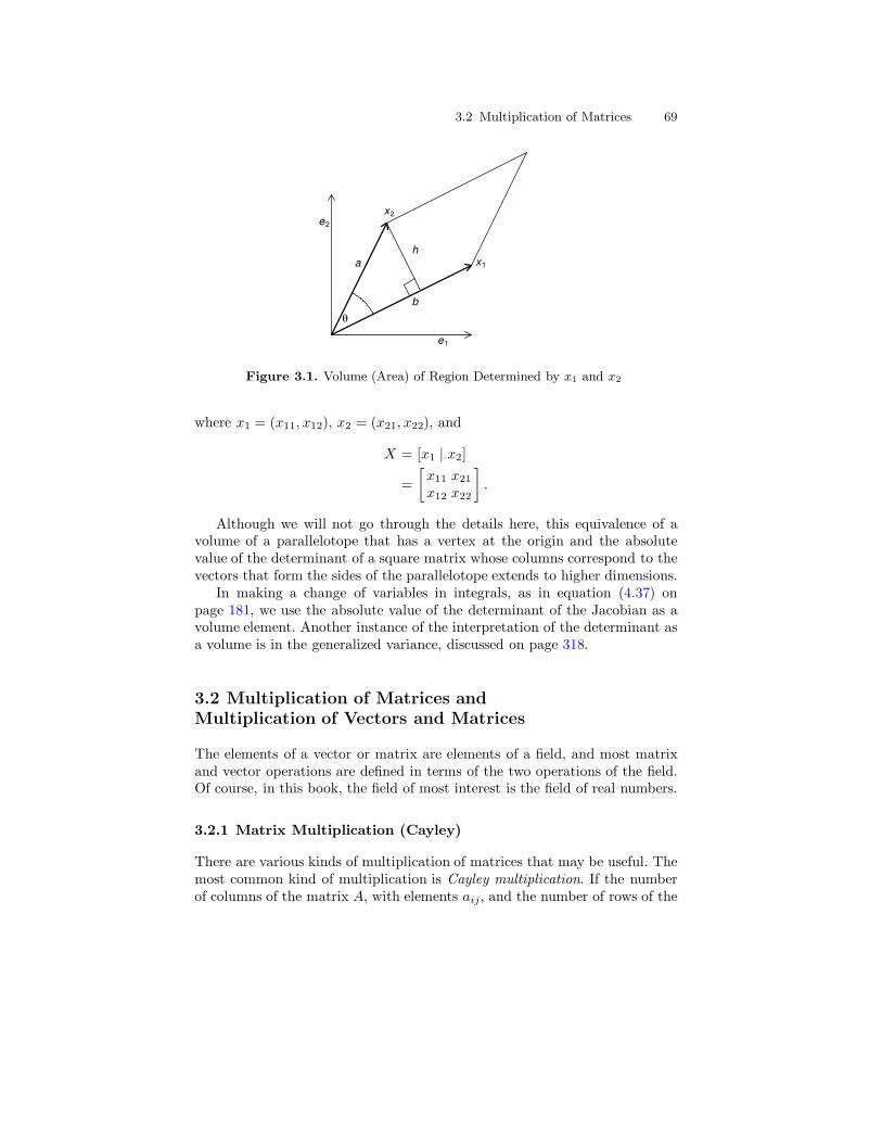
In Section 2.2, we discussed a useful geometric interpretation of vectors ina linear space with a Cartesian coordinate system. The elements of a vec-tor correspond to measurements along the respective axes of the coordinatesystem. When working with several vectors, or with a matrix in which thecolumns (or rows) are associated with vectors, we may designate a vectorxi as xi = (xi1, . . . , xid). A set of d linearly independent d-vectors define aparallelotope in d dimensions. For example, in a two-dimensional space, thelinearly independent 2-vectors x1 and x2 define a parallelogram, as shown inFigure 3.1.

The area of this parallelogram is the base times the height, bh, where, inthis case, b is the length of the vector x1, and h is the length of x2 times thesine of the angle θ. Thus, making use of equation (2.45) on page 36 for thecosine of the angle, we have

area = bh

= ‖x1‖‖x2‖ sin(θ)

= ‖x1‖‖x2‖√

1−( 〈x1, x2〉‖x1‖‖x2‖

)2

=√‖x1‖2‖x2‖2 − (〈x1, x2〉)2

=√

(x211 + x2

12)(x221 + x2

22)− (x11x21 − x12x22)2

= |x11x22 − x12x21|= |det(X)|, (3.36)

3.2 Multiplication of Matrices 69

x2

x1

θ

a

h

b

e1

e2

Figure 3.1. Volume (Area) of Region Determined by x1 and x2

where x1 = (x11, x12), x2 = (x21, x22), and

X = [x1 | x2]

=

[x11 x21

x12 x22

].

Although we will not go through the details here, this equivalence of avolume of a parallelotope that has a vertex at the origin and the absolutevalue of the determinant of a square matrix whose columns correspond to thevectors that form the sides of the parallelotope extends to higher dimensions.

In making a change of variables in integrals, as in equation (4.37) onpage 181, we use the absolute value of the determinant of the Jacobian as avolume element. Another instance of the interpretation of the determinant asa volume is in the generalized variance, discussed on page 318.

3.2 Multiplication of Matrices and

Multiplication of Vectors and Matrices

The elements of a vector or matrix are elements of a field, and most matrixand vector operations are defined in terms of the two operations of the field.Of course, in this book, the field of most interest is the field of real numbers.

3.2.1 Matrix Multiplication (Cayley)

There are various kinds of multiplication of matrices that may be useful. Themost common kind of multiplication is Cayley multiplication. If the numberof columns of the matrix A, with elements aij, and the number of rows of the


matrix B, with elements bij, are equal, then the (Cayley) product of A and Bis defined as the matrix C with elements

cij =∑

k

aikbkj. (3.37)

This is the most common type of matrix product, and we refer to it by theunqualified phrase “matrix multiplication”.

Cayley matrix multiplication is indicated by juxtaposition, with no inter-vening symbol for the operation: C = AB.

If the matrix A is n×m and the matrix B is m× p, the product C = ABis n× p:

C = A B

[ ]

n×p

=

[ ]

n×m

[ ]m×p

.

Cayley matrix multiplication is a mapping,

IRn×m × IRm×p 7→ IRn×p.

The multiplication of an n × m matrix and an m × p matrix requiresnmp scalar multiplications and np(m − 1) scalar additions. Here, as alwaysin numerical analysis, we must remember that the definition of an operation,such as matrix multiplication, does not necessarily define a good algorithmfor evaluating the operation.

It is obvious that while the product AB may be well-defined, the productBA is defined only if n = p; that is, if the matrices AB and BA are square.We assume throughout that writing a product of matrices AB implies thatthe number of columns of the first matrix is the same as the number of rows ofthe second; that is, they are conformable for multiplication in the order given.

It is easy to see from the definition of matrix multiplication (3.37) thatin general, even for square matrices, AB 6= BA. It is also obvious that if ABexists, then BTAT exists and, in fact,

BTAT = (AB)T. (3.38)

The product of symmetric matrices is not, in general, symmetric. If (but notonly if) A and B are symmetric, then AB = (BA)T.

Because matrix multiplication is not commutative, we often use the terms“premultiply” and “postmultiply” and the corresponding nominal forms ofthese terms. Thus, in the product AB, we may say B is premultiplied by A,or, equivalently, A is postmultiplied by B.

Although matrix multiplication is not commutative, it is associative; thatis, if the matrices are conformable,

A(BC) = (AB)C. (3.39)


It is also distributive over addition; that is,

A(B + C) = AB + AC (3.40)

and(B + C)A = BA + CA. (3.41)

These properties are obvious from the definition of matrix multiplication.(Note that left-sided distribution is not the same as right-sided distributionbecause the multiplication is not commutative.)

An n×n matrix consisting of 1s along the diagonal and 0s everywhere else isa multiplicative identity for the set of n×n matrices and Cayley multiplication.Such a matrix is called the identity matrix of order n, and is denoted by In,or just by I. The columns of the identity matrix are unit vectors.

The identity matrix is a multiplicative identity for any matrix so long asthe matrices are conformable for the multiplication. If A is n×m, then

InA = AIm = A.

Powers of Square Matrices

For a square matrix A, its product with itself is defined, and so we will use thenotation A2 to mean the Cayley product AA, with similar meanings for Ak

for a positive integer k. As with the analogous scalar case, Ak for a negativeinteger may or may not exist, and when it exists, it has a meaning for Cayleymultiplication similar to the meaning in ordinary scalar multiplication. Wewill consider these issues later (in Section 3.3.3).

For an n × n matrix A, if Ak exists for negative integral values of k, wedefine A0 by

A0 = In. (3.42)

For a diagonal matrix D = diag ((d1, . . . , dn)), we have

Dk = diag((dk

1 , . . . , dkn)). (3.43)

Matrix Polynomials

Polynomials in square matrices are similar to the more familiar polynomialsin scalars. We may consider

p(A) = b0I + b1A + · · · bkAk.

The value of this polynomial is a matrix.The theory of polynomials in general holds, and in particular, we have the

useful factorizations of monomials: for any positive integer k,

I −Ak = (I −A)(I + A + · · ·Ak−1), (3.44)

and for an odd positive integer k,

I + Ak = (I + A)(I −A + · · ·Ak−1). (3.45)


3.2.2 Multiplication of Matrices with Special Patterns

Various properties of matrices may or may not be preserved under matrixmultiplication. We have seen already that the product of symmetric matricesis not in general symmetric.

Many of the various patterns of zeroes in matrices discussed on page 53 arepreserved under matrix multiplication. Assume A and B are square matricesof the same number of rows.

• If A and B are diagonal, AB is diagonal;• if A and B are upper triangular, AB is upper triangular;• if A and B are lower triangular, AB is lower triangular;• if A is upper triangular and B is lower triangular, in general, none of

AB, BA, ATA, BTB, AAT, and BBT is triangular.

Each of these statements can be easily proven using the definition of multi-plication in equation (3.37).

The products of banded matrices are generally banded with a wider band-width. If the bandwidth is too great, obviously the matrix can no longer becalled banded.

Multiplication of Partitioned Matrices

Multiplication and other operations with partitioned matrices are carried outwith their submatrices in the obvious way. Thus, assuming the submatricesare conformable for multiplication,

[A11 A12

A21 A22

] [B11 B12

B21 B22

]=

[A11B11 + A12B21 A11B12 + A12B22

A21B11 + A22B21 A21B12 + A22B22

].

It is clear that the product of conformable block diagonal matrices is blockdiagonal.

Sometimes a matrix may be partitioned such that one partition is just asingle column or row, that is, a vector or the transpose of a vector. In thatcase, we may use a notation such as

[X y]

or[X | y],

where X is a matrix and y is a vector. We develop the notation in the obviousfashion; for example,

[X y]T [X y] =

[XTX XTyyTX yTy

]. (3.46)


3.2.3 Elementary Operations on Matrices

Many common computations involving matrices can be performed as a se-quence of three simple types of operations on either the rows or the columnsof the matrix:

• the interchange of two rows (columns),• a scalar multiplication of a given row (column), and• the replacement of a given row (column) by the sum of that row

(columns) and a scalar multiple of another row (column); that is, anaxpy operation.

Such an operation on the rows of a matrix can be performed by premultipli-cation by a matrix in a standard form, and an operation on the columns ofa matrix can be performed by postmultiplication by a matrix in a standardform. To repeat:

• premultiplication: operation on rows;• postmultiplication: operation on columns.

The matrix used to perform the operation is called an elementary trans-formation matrix or elementary operator matrix. Such a matrix is the identitymatrix transformed by the corresponding operation performed on its unitrows, eT

p , or columns, ep.In actual computations, we do not form the elementary transformation

matrices explicitly, but their formulation allows us to discuss the operationsin a systematic way and better understand the properties of the operations.Products of any of these elementary operator matrices can be used to effectmore complicated transformations.

Operations on the rows are more common, and that is what we will dis-cuss here, although operations on columns are completely analogous. Thesetransformations of rows are called elementary row operations.

Interchange of Rows or Columns; Permutation Matrices

By first interchanging the rows or columns of a matrix, it may be possibleto partition the matrix in such a way that the partitions have interestingor desirable properties. Also, in the course of performing computations on amatrix, it is often desirable to interchange the rows or columns of the matrix.(This is an instance of “pivoting”, which will be discussed later, especiallyin Chapter 6.) In matrix computations, we almost never actually move datafrom one row or column to another; rather, the interchanges are effected bychanging the indexes to the data.

Interchanging two rows of a matrix can be accomplished by premultiply-ing the matrix by a matrix that is the identity with those same two rowsinterchanged; for example,


1 0 0 00 0 1 00 1 0 00 0 0 1

a11 a12 a13

a21 a22 a23

a31 a32 a33

a41 a42 a43

=

a11 a12 a13

a31 a32 a33

a21 a22 a23

a41 a42 a43

.

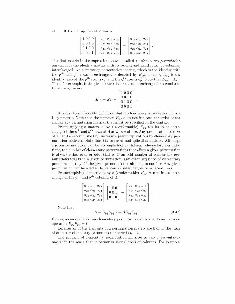
The first matrix in the expression above is called an elementary permutationmatrix. It is the identity matrix with its second and third rows (or columns)interchanged. An elementary permutation matrix, which is the identity withthe pth and qth rows interchanged, is denoted by Epq. That is, Epq is theidentity, except the pth row is eT

q and the qth row is eTp . Note that Epq = Eqp.

Thus, for example, if the given matrix is 4×m, to interchange the second andthird rows, we use

E23 = E32 =

1 0 0 00 0 1 00 1 0 00 0 0 1

.

It is easy to see from the definition that an elementary permutation matrixis symmetric. Note that the notation Epq does not indicate the order of theelementary permutation matrix; that must be specified in the context.

Premultiplying a matrix A by a (conformable) Epq results in an inter-change of the pth and qth rows of A as we see above. Any permutation of rowsof A can be accomplished by successive premultiplications by elementary per-mutation matrices. Note that the order of multiplication matters. Althougha given permutation can be accomplished by different elementary permuta-tions, the number of elementary permutations that effect a given permutationis always either even or odd; that is, if an odd number of elementary per-mutations results in a given permutation, any other sequence of elementarypermutations to yield the given permutation is also odd in number. Any givenpermutation can be effected by successive interchanges of adjacent rows.

Postmultiplying a matrix A by a (conformable) Epq results in an inter-change of the pth and qth columns of A:

a11 a12 a13

a21 a22 a23

a31 a32 a33

a41 a42 a43

1 0 00 0 10 1 0

=

a11 a13 a12

a21 a23 a22

a31 a33 a32

a41 a43 a42

.

Note thatA = EpqEpqA = AEpqEpq; (3.47)

that is, as an operator, an elementary permutation matrix is its own inverseoperator: EpqEpq = I.

Because all of the elements of a permutation matrix are 0 or 1, the traceof an n × n elementary permutation matrix is n− 2.

The product of elementary permutation matrices is also a permutationmatrix in the sense that it permutes several rows or columns. For example,


premultiplying A by the matrix Q = EpqEqr will yield a matrix whose pth rowis the rth row of the original A, whose qth row is the pth row of A, and whoserth row is the qth row of A. We often use the notation Eπ to denote a moregeneral permutation matrix. This expression will usually be used generically,but sometimes we will specify the permutation, π.

A general permutation matrix (that is, a product of elementary permuta-tion matrices) is not necessarily symmetric, but its transpose is also a per-mutation matrix. It is not necessarily its own inverse, but its permutationscan be reversed by a permutation matrix formed by products of elementarypermutation matrices in the opposite order; that is,

ETπ Eπ = I.

As a prelude to other matrix operations, we often permute both rows andcolumns, so we often have a representation such as

B = Eπ1AEπ2

, (3.48)

where Eπ1is a permutation matrix to permute the rows and Eπ2

is a permu-tation matrix to permute the columns. We use these kinds of operations toarrive at the important equation (3.105) on page 93, and combine these oper-ations with others to yield equation (3.119) on page 99. These equations areused to determine the number of linearly independent rows and columns andto represent the matrix in a form with a maximal set of linearly independentrows and columns clearly identified.

The Vec-Permutation Matrix

A special permutation matrix is the matrix that transforms the vector vec(A)into vec(AT). If A is n×m, the matrix Knm that does this is nm× nm. Wehave

vec(AT) = Knmvec(A). (3.49)

The matrix Knm is called the nm vec-permutation matrix.

Scalar Row or Column Multiplication

Often, numerical computations with matrices are more accurate if the rowshave roughly equal norms. For this and other reasons, we often transform amatrix by multiplying one of its rows by a scalar. This transformation can alsobe performed by premultiplication by an elementary transformation matrix.For multiplication of the pth row by the scalar, the elementary transformationmatrix, which is denoted by Ep(a), is the identity matrix in which the pth

diagonal element has been replaced by a. Thus, for example, if the givenmatrix is 4×m, to multiply the second row by a, we use


E2(a) =

1 0 0 00 a 0 00 0 1 00 0 0 1

.

Postmultiplication of a given matrix by the multiplier matrix Ep(a) resultsin the multiplication of the pth column by the scalar. For this, Ep(a) is a squarematrix of order equal to the number of columns of the given matrix.

Note that the notation Ep(a) does not indicate the number of rows andcolumns. This must be specified in the context.

Note that, if a 6= 0,A = Ep(1/a)Ep(a)A, (3.50)

that is, as an operator, the inverse operator is a row multiplication matrix onthe same row and with the reciprocal as the multiplier.

Axpy Row or Column Transformations

The other elementary operation is an axpy on two rows and a replacement ofone of those rows with the result

ap ← aaq + ap.

This operation also can be effected by premultiplication by a matrix formedfrom the identity matrix by inserting the scalar in the (p, q) position. Such amatrix is denoted by Epq(a). Thus, for example, if the given matrix is 4×m,to add a times the third row to the second row, we use

E23(a) =

1 0 0 00 1 a 00 0 1 00 0 0 1

.

Premultiplication of a matrix A by such a matrix,

Epq(a)A, (3.51)

yields a matrix whose pth row is a times the qth row plus the original row.Given the 4× 3 matrix A = (aij), we have

E23(a)A =

a11 a12 a13

a21 + aa31 a22 + aa32 a23 + aa33

a31 a32 a33

a41 a42 a43

.

Postmultiplication of a matrix A by an axpy operator matrix,

AEpq(a),


yields a matrix whose qth column is a times the pth column plus the originalcolumn. For this, Epq(a) is a square matrix of order equal to the number ofcolumns of the given matrix. Note that the column that is changed correspondsto the second subscript in Epq(a).

Note thatA = Epq(−a)Epq(a)A; (3.52)

that is, as an operator, the inverse operator is the same axpy elementaryoperator matrix with the negative of the multiplier.

A common use of axpy operator matrices is to form a matrix with zerosin all positions of a given column below a given position in the column. Theseoperations usually follow an operation by a scalar row multiplier matrix thatputs a 1 in the position of interest. For example, given an n × m matrix Awith aij 6= 0, to put a 1 in the (i, j) position and 0s in all positions of the jth

column below the ith row, we form the product

Emi(−amj) · · ·Ei+1,i(−ai+1,j)Ei(1/aij)A. (3.53)

This process is called Gaussian elimination.Gaussian elimination is often performed sequentially down the diagonal

elements of a matrix. If at some point aii = 0, the operations of equation (3.53)cannot be performed. In that case, we may first interchange the ith row withthe kth row, where k > i and aki 6= 0. Such an interchange is called pivoting.We will discuss pivoting in more detail on page 229 in Chapter 6.

To form a matrix with zeros in all positions of a given column except one,we use additional matrices for the rows above the given element:

Emi(−amj) · · ·Ei+1,i(−ai+1,j) · · ·Ei−1,i(−ai−1,j) · · ·E1i(−a1j)Ei(1/aij)A.

We can likewise zero out all elements in the ith row except the one in the(ij)th position by similar postmultiplications.

These elementary transformations are the basic operations in Gaussianelimination, which is discussed in Sections 5.6 and 6.2.1.

Elementary Operator Matrices: Summary of Notation

Because we have introduced various notation for elementary operator matri-ces, it may be worthwhile to review the notation. The notation is useful andI will use it from time to time, but unfortunately, there is no general form forthe notation. I will generally use an “E” as the root symbol for the matrix,but the specific type is indicated by various other symbols.

Referring back to the listing of the types of operations on page 73, we havethe various elementary operator matrices:

• Epq: the interchange of rows p and q (Epq is the same as Eqp)Eπ: a general permutation of rows, where π denotes a permutation

• Ep(a): multiplication of row p by a.


• Epq(a): the replacement of row p by the sum of row p and a times row q.

Recall that these operations are effected by premultiplication. The same kindsof operations on the columns are effected by postmultiplication.

Determinants of Elementary Operator Matrices

The determinant of an elementary permutation matrix Epq has only one termin the sum that defines the determinant (equation (3.18), page 61), and thatterm is 1 times σ evaluated at the permutation that exchanges p and q. Aswe have seen (page 61), this is an odd permutation; hence, for an elementarypermutation matrix Epq,

det(Epq) = −1. (3.54)

Because all terms in det(EpqA) are exactly the same terms as in det(A)but with one different permutation in each term, we have

det(EpqA) = −det(A).

More generally, if A and Eπ are n × n matrices, and Eπ is any permutationmatrix (that is, any product of Epq matrices), then det(EπA) is either det(A)or −det(A) because all terms in det(EπA) are exactly the same as the termsin det(A) but possibly with different signs because the permutations are dif-ferent. In fact, the differences in the permutations are exactly the same as thepermutation of 1, . . . , n in Eπ; hence,

det(EπA) = det(Eπ) det(A).

(In equation (3.60) below, we will see that this equation holds more generally.)The determinant of an elementary row multiplication matrix Ep(a) is

det(Ep(a)) = a. (3.55)

If A and Ep(a) are n× n matrices, then

det(Ep(a)A) = adet(A),

as we see from the definition of the determinant, equation (3.18).The determinant of an elementary axpy matrix Epq(a) is 1,

det(Epq(a)) = 1, (3.56)

because the term consisting of the product of the diagonals is the only termin the determinant.

Now consider det(Epq(a)A) for an n×n matrix A. Expansion in the minors(equation (3.24)) along the pth row yields


det(Epq(a)A) =

n∑

j=1

(apj + aaqj)(−1)p+jdet(A(ij))

=

n∑

j=1

apj(−1)p+jdet(A(ij)) + a

n∑

j=1

aqj(−1)p+jdet(A(ij)).

From equation (3.26) on page 64, we see that the second term is 0, and sincethe first term is just the determinant of A, we have

det(Epq(a)A) = det(A). (3.57)

3.2.4 The Trace of a Cayley Product that Is Square

A useful property of the trace for the matrices A and B that are conformablefor the multiplications AB and BA is

tr(AB) = tr(BA). (3.58)

This is obvious from the definitions of matrix multiplication and the trace.Note that A and B may not be square (so the trace is not defined for them),but if they are conformable for the multiplications, then both AB and BAare square.

Because of the associativity of matrix multiplication, this relation can beextended as

tr(ABC) = tr(BCA) = tr(CAB) (3.59)

for matrices A, B, and C that are conformable for the multiplications indi-cated. Notice that the individual matrices need not be square. This fact isvery useful in working with quadratic forms, as in equation (3.68).

3.2.5 The Determinant of a Cayley Product of Square Matrices

An important property of the determinant is

det(AB) = det(A) det(B) (3.60)

if A and B are square matrices conformable for multiplication. We see this byfirst forming

det

([I A0 I

] [A 0−I B

])= det

([0 AB−I B

])(3.61)

and then observing from equation (3.33) that the right-hand side is det(AB).Now consider the left-hand side. The matrix that is the first factor on theleft-hand side is a product of elementary axpy transformation matrices; thatis, it is a matrix that when postmultiplied by another matrix merely addsmultiples of rows in the lower part of the matrix to rows in the upper part of


the matrix. If A and B are n × n (and so the identities are likewise n × n),the full matrix is the product:

[I A0 I

]= E1,n+1(a11) · · ·E1,2n(a1n)E2,n+1(a21) · · ·E2,2n(a2,n) · · ·En,2n(ann).

Hence, applying equation (3.57) recursively, we have

det

([I A0 I

] [A 0−I B

])= det

([A 0−I B

]),

and from equation (3.32) we have

det

([A 0−I B

])= det(A)det(B),

and so finally we have equation (3.60).From equation (3.60), we see that if A and B are square matrices con-

formable for multiplication, then

det(AB) = det(BA). (3.62)

(Recall, in general, even in the case of square matrices, AB 6= BA.) Thisequation is to be contrasted with equation (3.58), tr(AB) = tr(BA), whichdoes not even require that the matrices be square. A simple counterexamplefor nonsquare matrices is det(xxT) 6= det(xTx), where x is a vector withat least two elements. (Here, think of the vector as an n × 1 matrix. Thiscounterexample can be seen in various ways. One way is to use a fact that wewill encounter on page 105, and observe that det(xxT) = 0 for any x with atleast two elements.)

3.2.6 Multiplication of Matrices and Vectors

It is often convenient to think of a vector as a matrix with only one ele-ment in one of its dimensions. This provides for an immediate extension ofthe definitions of transpose and matrix multiplication to include vectors aseither or both factors. In this scheme, we follow the convention that a vectorcorresponds to a column; that is, if x is a vector and A is a matrix, Ax orxTA may be well-defined, but neither xA nor AxT would represent anything,except in the case when all dimensions are 1. (In some computer systems formatrix algebra, these conventions are not enforced; see, for example the Rcode in Figure 12.4 on page 491.) The alternative notation xTy we introducedearlier for the dot product or inner product, 〈x, y〉, of the vectors x and y isconsistent with this paradigm.

Vectors and matrices are fundamentally different kinds of mathematicalobjects. In general, it is not relevant to say that a vector is a “column” or


a “row”; it is merely a one-dimensional (or rank 1) object. We will continueto write vectors as x = (x1, . . . , xn), but this does not imply that the vectoris a “row vector”. Matrices with just one row or one column are differentobjects from vectors. We represent a matrix with one row in a form such asY = [y11 . . . y1n], and we represent a matrix with one column in a form such

as Z =

z11

...zm1

or as Z = [z11 . . . zm1]

T.

(Compare the notation in equations (1.1) and (1.2) on page 4.)

The Matrix/Vector Product as a Linear Combination

If we represent the vectors formed by the columns of an n × m matrix Aas a1, . . . , am, the matrix/vector product Ax is a linear combination of thesecolumns of A:

Ax =

m∑

i=1

xiai. (3.63)

(Here, each xi is a scalar, and each ai is a vector.)Given the equation Ax = b, we have b ∈ span(A); that is, the n-vector b

is in the k-dimensional column space of A, where k ≤ m.

3.2.7 Outer Products

The outer product of the vectors x and y is the matrix

xyT. (3.64)

Note that the definition of the outer product does not require the vectors tobe of equal length. Note also that while the inner product is commutative,the outer product is not commutative (although it does have the propertyxyT = (yxT)T).

A very common outer product is of a vector with itself:

xxT.

The outer product of a vector with itself is obviously a symmetric matrix.We should again note some subtleties of differences in the types of objects

that result from operations. If A and B are matrices conformable for theoperation, the product ATB is a matrix even if both A and B are n × 1 andso the result is 1 × 1. For the vectors x and y and matrix C, however, xTyand xTCy are scalars; hence, the dot product and a quadratic form are notthe same as the result of a matrix multiplication. The dot product is a scalar,and the result of a matrix multiplication is a matrix. The outer product ofvectors is a matrix, even if both vectors have only one element. Nevertheless,as we have mentioned before, we will treat a one by one matrix or a vectorwith only one element as a scalar whenever it is convenient to do so.


3.2.8 Bilinear and Quadratic Forms; Definiteness

A variation of the vector dot product, xTAy, is called a bilinear form, andthe special bilinear form xTAx is called a quadratic form. Although in thedefinition of quadratic form we do not require A to be symmetric— becausefor a given value of x and a given value of the quadratic form xTAx there is aunique symmetric matrix As such that xTAsx = xTAx —we generally workonly with symmetric matrices in dealing with quadratic forms. (The matrixAs is 1

2(A + AT); see Exercise 3.3.) Quadratic forms correspond to sums of

squares and hence play an important role in statistical applications.

Nonnegative Definite and Positive Definite Matrices

A symmetric matrix A such that for any (conformable and real) vector x thequadratic form xTAx is nonnegative, that is,

xTAx ≥ 0, (3.65)

is called a nonnegative definite matrix. We denote the fact that A is nonneg-ative definite by

A � 0.

(Note that we consider 0n×n to be nonnegative definite.)A symmetric matrix A such that for any (conformable) vector x 6= 0 the

quadratic formxTAx > 0 (3.66)

is called a positive definite matrix. We denote the fact that A is positivedefinite by

A � 0.

(Recall that A ≥ 0 and A > 0 mean, respectively, that all elements of A arenonnegative and positive.) When A and B are symmetric matrices of the sameorder, we write A � B to mean A − B � 0 and A � B to mean A − B � 0.Nonnegative and positive definite matrices are very important in applications.We will encounter them from time to time in this chapter, and then we willdiscuss more of their properties in Section 8.3.

In this book we use the terms “nonnegative definite” and “positive defi-nite” only for symmetric matrices. In other literature, these terms may be usedmore generally; that is, for any (square) matrix that satisfies (3.65) or (3.66).

The Trace of Inner and Outer Products

The invariance of the trace to permutations of the factors in a product (equa-tion (3.58)) is particularly useful in working with bilinear and quadratic forms.Let A be an n×m matrix, x be an n-vector, and y be an m-vector. Because


the bilinear form is a scalar (or a 1×1 matrix), and because of the invariance,we have the very useful fact

xTAy = tr(xTAy)

= tr(AyxT). (3.67)

A common instance is when A is square and x = y. We have for the quadraticform the equality

xTAx = tr(AxxT). (3.68)

In equation (3.68), if A is the identity I, we have that the inner product ofa vector with itself is the trace of the outer product of the vector with itself,that is,

xTx = tr(xxT). (3.69)

Also, by letting A be the identity in equation (3.68), we have an alternativeway of showing that for a given vector x and any scalar a, the norm ‖x− a‖is minimized when a = x:

(x− a)T(x − a) = tr(xcxTc ) + n(a− x)2. (3.70)

(Here, “x” denotes the mean of the elements in x. Compare this with equa-tion (2.61) on page 44.)

3.2.9 Anisometric Spaces

In Section 2.1, we considered various properties of vectors that depend onthe inner product, such as orthogonality of two vectors, norms of a vector,angles between two vectors, and distances between two vectors. All of theseproperties and measures are invariant to the orientation of the vectors; thespace is isometric with respect to a Cartesian coordinate system. Noting thatthe inner product is the bilinear form xTIy, we have a heuristic generalizationto an anisometric space. Suppose, for example, that the scales of the coordi-nates differ; say, a given distance along one axis in the natural units of theaxis is equivalent (in some sense depending on the application) to twice thatdistance along another axis, again measured in the natural units of the axis.The properties derived from the inner product, such as a norm and a metric,may correspond to the application better if we use a bilinear form in whichthe matrix reflects the different effective distances along the coordinate axes.A diagonal matrix whose entries have relative values corresponding to theinverses of the relative scales of the axes may be more useful. Instead of xTy,we may use xTDy, where D is this diagonal matrix.

Rather than differences in scales being just in the directions of the co-ordinate axes, more generally we may think of anisometries being measuredby general (but perhaps symmetric) matrices. (The covariance and correlationmatrices defined on page 316 come to mind. Any such matrix to be used in this


context should be positive definite because we will generalize the dot prod-uct, which is necessarily nonnegative, in terms of a quadratic form.) A bilinearform xTAy may correspond more closely to the properties of the applicationthan the standard inner product.

We define orthogonality of two vectors x and y with respect to A by

xTAy = 0. (3.71)

In this case, we say x and y are A-conjugate.The L2 norm of a vector is the square root of the quadratic form of the

vector with respect to the identity matrix. A generalization of the L2 vectornorm, called an elliptic norm or a conjugate norm, is defined for the vectorx as the square root of the quadratic form xTAx for any symmetric positivedefinite matrix A. It is sometimes denoted by ‖x‖A:

‖x‖A =√

xTAx. (3.72)

It is easy to see that‖x‖A

satisfies the definition of a norm given on page 24. If A is a diagonal matrixwith elements wi ≥ 0, the elliptic norm is the weighted L2 norm of equa-tion (2.31).

The elliptic norm yields an elliptic metric in the usual way of defining ametric in terms of a norm. The distance between the vectors x and y withrespect to A is

√(x− y)TA(x− y). It is easy to see that this satisfies the

definition of a metric given on page 30.A metric that is widely useful in statistical applications is the Mahalanobis

distance, which uses a covariance matrix as the scale for a given space. (Thesample covariance matrix is defined in equation (8.70) on page 316.) If S isthe covariance matrix, the Mahalanobis distance, with respect to that matrix,between the vectors x and y is

√(x− y)TS−1(x− y). (3.73)

3.2.10 Other Kinds of Matrix Multiplication

The most common kind of product of two matrices is the Cayley product,and when we speak of matrix multiplication without qualification, we meanthe Cayley product. Three other types of matrix multiplication that are use-ful are Hadamard multiplication, Kronecker multiplication, and inner productmultiplication.

The Hadamard Product

Hadamard multiplication is defined for matrices of the same shape as the mul-tiplication of each element of one matrix by the corresponding element of the


other matrix. Hadamard multiplication immediately inherits the commutativ-ity, associativity, and distribution over addition of the ordinary multiplicationof the underlying field of scalars. Hadamard multiplication is also called arraymultiplication and element-wise multiplication. Hadamard matrix multiplica-tion is a mapping

IRn×m × IRn×m 7→ IRn×m.

The identity for Hadamard multiplication is the matrix of appropriateshape whose elements are all 1s.

The Kronecker Product

Kronecker multiplication, denoted by ⊗, is defined for any two matrices An×m

and Bp×q as

A⊗B =

a11B . . . a1mB... . . .

...an1B . . . anmB

.

The Kronecker product of A and B is np × mq; that is, Kronecker matrixmultiplication is a mapping

IRn×m × IRp×q 7→ IRnp×mq.

The Kronecker product is also called the “right direct product” or justdirect product. (A left direct product is a Kronecker product with the factorsreversed. In some of the earlier literature, “Kronecker product” was used tomean a left direct product.) Note the similarity of the Kronecker product ofmatrices with the direct product of sets, defined on page 5, in the sense thatthe result is formed from ordered pairs of elements from the two operands.

Kronecker multiplication is not commutative, but it is associative and itis distributive over addition, as we will see below. (Again, this parallels thedirect product of sets.)

The identity for Kronecker multiplication is the 1 × 1 matrix with theelement 1; that is, it is the same as the scalar 1.

We can understand the properties of the Kronecker product by expressingthe (i, j) element of A⊗ B in terms of the elements of A and B,

(A⊗ B)i,j = A[i/p]+1, [j/q]+1Bi−p[i/p], j−q[i/q], (3.74)

where [·] is the greatest integer function.Some additional properties of Kronecker products that are immediate re-

sults of the definition are, assuming the matrices are conformable for theindicated operations,


(aA) ⊗ (bB) = ab(A ⊗B)

= (abA) ⊗B

= A ⊗ (abB), for scalars a, b, (3.75)

(A + B) ⊗ (C) = A ⊗C + B ⊗ C, (3.76)

(A⊗ B) ⊗C = A ⊗ (B ⊗ C), (3.77)

(A⊗ B)T = AT ⊗ BT, (3.78)

(A ⊗B)(C ⊗D) = AC ⊗ BD. (3.79)

These properties are all easy to see by using equation (3.74) to express the(i, j) element of the matrix on either side of the equation, taking into accountthe size of the matrices involved. For example, in the first equation, if A isn×m and B is p× q, the (i, j) element on the left-hand side is

aA[i/p]+1, [j/q]+1bBi−p[i/p], j−q[i/q]

and that on the right-hand side is

abA[i/p]+1, [j/q]+1Bi−p[i/p], j−q[i/q].

They are all this easy! Hence, they are Exercise 3.6.The determinant of the Kronecker product of two square matrices An×n

and Bm×m has a simple relationship to the determinants of the individualmatrices:

det(A ⊗B) = det(A)mdet(B)n . (3.80)

The proof of this, like many facts about determinants, is straightforward butinvolves tedious manipulation of cofactors. The manipulations in this case canbe facilitated by using the vec-permutation matrix. See Harville (1997) for adetailed formal proof.

Another property of the Kronecker product of square matrices is

tr(A⊗ B) = tr(A)tr(B). (3.81)

This is true because the trace of the product is merely the sum of all possibleproducts of the diagonal elements of the individual matrices.

The Kronecker product and the vec function often find uses in the sameapplication. For example, an n×m normal random matrix X with parametersM , Σ, and Ψ can be expressed in terms of an ordinary np-variate normalrandom variable Y = vec(X) with parameters vec(M) and Σ⊗Ψ . (We discussmatrix random variables briefly on page 185. For a fuller discussion, the readeris referred to a text on matrix random variables such as Carmeli, 1983.)


A relationship between the vec function and Kronecker multiplication is

vec(ABC) = (CT ⊗A)vec(B) (3.82)

for matrices A, B, and C that are conformable for the multiplication indicated.

The Inner Product of Matrices

A product of two matrices of the same shape is defined as the sum of thedot products of the vectors formed from the columns of one matrix withvectors formed from the corresponding columns of the other matrix; that is,if a1, . . . , am are the columns of A and b1, . . . , bm are the columns of B, thenthe inner product of A and B, denoted 〈A, B〉, is

〈A, B〉 =

m∑

j=1

aTj bj. (3.83)

Similarly as for vectors (page 23), the inner product is sometimes called a “dotproduct”, and the notation A ·B is sometimes used to denote the matrix innerproduct. (I generally try to avoid use of the term dot product for matricesbecause the term may be used differently by different people. In Matlab, forexample, “dot product”, implemented in the dot function, can refer either to1×m matrix consisting of the individual terms in the sum in equation (3.83),or to the n×1 matrix consisting of the the dot products of the vectors formedfrom the rows of A and B. In the NumPy linear algebra package, the dot

function implements Cayley multiplication! This is probably because someoneworking with Python realized the obvious fact that the defining equation ofCayley multiplication, equation (3.37) on page 70, is actually the dot productof the vector formed from the elements in the ith row in the first matrix andthe vector formed from the elements in the jth column in the first matrix.)

For conformable matrices A, B, and C, we can easily confirm that thisproduct satisfies the general properties of an inner product listed on page 23:

• If A 6= 0, 〈A, A〉 > 0, and 〈0, A〉 = 〈A, 0〉 = 〈0, 0〉 = 0.• 〈A, B〉 = 〈B, A〉.• 〈sA, B〉 = s〈A, B〉, for a scalar s.• 〈(A + B), C〉 = 〈A, C〉+ 〈B, C〉.As in the case of the inner product of vectors, the inner product of matricesdefined as in equation (3.83) over the complex field is not an inner productbecause the first property listed above does not hold. As in the case of vectors,a generalized definition of a inner product using complex conjugates is an innerproduct.

As with any inner product (restricted to objects in the field of the reals),its value is a real number. Thus the matrix inner product is a mapping

IRn×m × IRn×m 7→ IR.


We see from the definition above that the inner product of matrices satisfies

〈A, B〉 = tr(ATB), (3.84)

which could alternatively be taken as the definition.Rewriting the definition of 〈A, B〉 as

∑mj=1

∑ni=1 aijbij, we see that

〈A, B〉 = 〈AT, BT〉. (3.85)

Like any inner product, inner products of matrices obey the Cauchy-Schwarz inequality (see inequality (2.21), page 24),

〈A, B〉 ≤ 〈A, A〉 12 〈B, B〉 12 , (3.86)

with equality holding only if A = 0 or B = sA for some scalar s.In Section 2.1.8, we defined orthogonality and orthonormality of two or

more vectors in terms of inner products. We can likewise define an orthogonalbinary relationship between two matrices in terms of inner products of matri-ces. We say the matrices A and B of the same shape are orthogonal to eachother if

〈A, B〉 = 0. (3.87)

We also use the term “orthonormal” to refer to matrices that are orthogonalto each other and for which each has an inner product with itself of 1. InSection 3.7, we will define orthogonality as a unary property of matrices. Theterm “orthogonal”, when applied to matrices, generally refers to that propertyrather than the binary property we have defined here.

On page 59 we identified a vector space of matrices and defined a basisfor the space IRn×m. If {U1, . . . , Uk} is a basis set for M ⊂ IRn×m, with theproperty that 〈Ui, Uj〉 = 0 for i 6= j and 〈Ui, Ui〉 = 1, and A is an n × mmatrix, with the Fourier expansion

A =

k∑

i=1

ciUi, (3.88)

we have, analogous to equation (2.50) on page 39,

ci = 〈A, Ui〉. (3.89)

The ci have the same properties (such as the Parseval identity, equation (2.51),for example) as the Fourier coefficients in any orthonormal expansion. Bestapproximations within M can also be expressed as truncations of the sumin equation (3.88) as in equation (2.54). The objective of course is to reducethe truncation error. (The norms in Parseval’s identity and in measuring thegoodness of an approximation are matrix norms in this case. We discuss matrixnorms in Section 3.9 beginning on page 145.)

3.3 Matrix Rank and the Inverse of a Matrix 89

3.3 Matrix Rank and the Inverse of a Matrix

The linear dependence or independence of the vectors forming the rows orcolumns of a matrix is an important characteristic of the matrix.

The maximum number of linearly independent vectors (those forming ei-ther the rows or the columns) is called the rank of the matrix. We use thenotation

rank(A)

to denote the rank of the matrix A. (We have used the term “rank” before todenote dimensionality of an array. “Rank” as we have just defined it appliesonly to a matrix or to a set of vectors, and this is by far the more commonmeaning of the word. The meaning is clear from the context, however.)

Because multiplication by a nonzero scalar does not change the linearindependence of vectors, for the scalar a with a 6= 0, we have

rank(aA) = rank(A). (3.90)

From results developed in Section 2.1, we see that for the n ×m matrixA,

rank(A) ≤ min(n, m). (3.91)

Row Rank and Column Rank

We have defined matrix rank in terms of numbers of linearly independent rowsor columns. This is because the number of linearly independent rows is thesame as the number of linearly independent columns. Although we may usethe terms “row rank” or “column rank”, the single word “rank” is sufficientbecause they are the same. To see this, assume we have an n ×m matrix Aand that there are exactly p linearly independent rows and exactly q linearlyindependent columns. We can permute the rows and columns of the matrixso that the first p rows are linearly independent rows and the first q columnsare linearly independent and the remaining rows or columns are linearly de-pendent on the first ones. (Recall that applying the same permutation to allof the elements of each vector in a set of vectors does not change the lineardependencies over the set.) After these permutations, we have a matrix Bwith submatrices W , X, Y , and Z,

B =

[Wp×q Xp×m−q

Yn−p×q Zn−p×m−q

], (3.92)

where the rows of R = [W |X] correspond to p linearly independent m-vectors

and the columns of C =

[WY

]correspond to q linearly independent n-vectors.

Without loss of generality, we can assume p ≤ q. Now, if p < q, it must bethe case that the columns of W are linearly dependent because there are q of


them, but they have only p elements. Therefore, there is some q-vector a suchthat Wa = 0. Now, since the rows of R are the full set of linearly independentrows, any row in [Y |Z] can be expressed as a linear combination of the rowsof R, and any row in Y can be expressed as a linear combination of the rowsof W . This means, for some n−p × p matrix T , that Y = TW . In this case,however, Ca = 0. But this contradicts the assumption that the columns ofC are linearly independent; therefore it cannot be the case that p < q. Weconclude therefore that p = q; that is, that the maximum number of linearlyindependent rows is the same as the maximum number of linearly independentcolumns.

Because the row rank, the column rank, and the rank of A are all thesame, we have

rank(A) = dim(V(A)), (3.93)

rank(AT) = rank(A), (3.94)

dim(V(AT)) = dim(V(A)). (3.95)

(Note, of course, that in general V(AT) 6= V(A); the orders of the vector spacesare possibly different.)

Full Rank Matrices

If the rank of a matrix is the same as its smaller dimension, we say the matrixis of full rank. In the case of a nonsquare matrix, we may say the matrix isof full row rank or full column rank just to emphasize which is the smallernumber.

If a matrix is not of full rank, we say it is rank deficient and define therank deficiency as the difference between its smaller dimension and its rank.

A full rank matrix that is square is called nonsingular, and one that is notnonsingular is called singular.

A square matrix that is either row or column diagonally dominant is non-singular. The proof of this is Exercise 3.8. (It’s easy!)

A positive definite matrix is nonsingular. The proof of this is Exercise 3.9.

Later in this section, we will identify additional properties of square fullrank matrices. (For example, they have inverses and their determinants arenonzero.)

Rank of Elementary Operator Matrices and Matrix ProductsInvolving Them

Because within any set of rows of an elementary operator matrix (see Sec-tion 3.2.3), for some given column, only one of those rows contains a nonzero


element, the elementary operator matrices are all obviously of full rank (withthe proviso that a 6= 0 in Ep(a)).

Furthermore, the rank of the product of any given matrix with an elemen-tary operator matrix is the same as the rank of the given matrix. To see this,consider each type of elementary operator matrix in turn. For a given matrixA, the set of rows of EpqA is the same as the set of rows of A; hence, the rankof EpqA is the same as the rank of A. Likewise, the set of columns of AEpq

is the same as the set of columns of A; hence, again, the rank of AEpq is thesame as the rank of A.

The set of rows of Ep(a)A for a 6= 0 is the same as the set of rows of A,except for one, which is a nonzero scalar multiple of the corresponding rowof A; therefore, the rank of Ep(a)A is the same as the rank of A. Likewise,the set of columns of AEp(a) is the same as the set of columns of A, exceptfor one, which is a nonzero scalar multiple of the corresponding row of A;therefore, again, the rank of AEp(a) is the same as the rank of A.

Finally, the set of rows of Epq(a)A for a 6= 0 is the same as the set ofrows of A, except for one, which is a nonzero scalar multiple of some row ofA added to the corresponding row of A; therefore, the rank of Epq(a)A is thesame as the rank of A. Likewise, we conclude that the rank of AEpq(a) is thesame as the rank of A.

We therefore have that if P and Q are the products of elementary operatormatrices,

rank(PAQ) = rank(A). (3.96)

On page 101, we will extend this result to products by any full rank matrices.

3.3.1 The Rank of Partitioned Matrices, Products ofMatrices, and Sums of Matrices

The partitioning in equation (3.92) leads us to consider partitioned matricesin more detail.

Rank of Partitioned Matrices and Submatrices

Let the matrix A be partitioned as

A =

[A11 A12

A21 A22

],

where any pair of submatrices in a column or row may be null (that is, wherefor example, it may be the case that A = [A11|A12]). Then the number oflinearly independent rows of A must be at least as great as the number oflinearly independent rows of [A11|A12] and the number of linearly independentrows of [A21|A22]. By the properties of subvectors in Section 2.1.1, the numberof linearly independent rows of [A11|A12] must be at least as great as thenumber of linearly independent rows of A11 or A21. We could go through a


similar argument relating to the number of linearly independent columns andarrive at the inequality

rank(Aij) ≤ rank(A). (3.97)

Furthermore, we see that

rank(A) ≤ rank([A11|A12]) + rank([A21|A22]) (3.98)

because rank(A) is the number of linearly independent columns of A, whichis less than or equal to the number of linearly independent rows of [A11|A12]plus the number of linearly independent rows of [A12|A22]. Likewise, we have

rank(A) ≤ rank

([A11

A21

])+ rank

([A12

A22

]). (3.99)

In a similar manner, by merely counting the number of independent rows,we see that, if

V([A11|A12]

T)⊥ V

([A21|A22]

T),

thenrank(A) = rank([A11|A12]) + rank([A21|A22]); (3.100)

and, if

V([

A11

A21

])⊥ V

([A12

A22

]),

then

rank(A) = rank

([A11

A21

])+ rank

([A12

A22

]). (3.101)

An Upper Bound on the Rank of Products of Matrices

The rank of the product of two matrices is less than or equal to the lesser ofthe ranks of the two:

rank(AB) ≤ min(rank(A), rank(B)). (3.102)

We can show this by separately considering two cases for the n× k matrix Aand the k ×m matrix B. In one case, we assume k is at least as large as nand n ≤ m, and in the other case we assume k < n ≤ m. In both cases, werepresent the rows of AB as k linear combinations of the rows of B.

From equation (3.102), we see that the rank of an outer product matrix(that is, a matrix formed as the outer product of two vectors) is 1.

Equation (3.102) provides a useful upper bound on rank(AB). In Sec-tion 3.3.8, we will develop a lower bound on rank(AB).


An Upper and a Lower Bound on the Rank of Sums of Matrices

The rank of the sum of two matrices is less than or equal to the sum of theirranks; that is,

rank(A + B) ≤ rank(A) + rank(B). (3.103)

We can see this by observing that

A + B = [A|B]

[II

],

and so rank(A + B) ≤ rank([A|B]) by equation (3.102), which in turn is≤ rank(A) + rank(B) by equation (3.98).

Using inequality (3.103) and the fact that rank(−B) = rank(B), we writerank(A−B) ≤ rank(A)+rank(B), and so, replacing A in (3.103) by A+B, wehave rank(A) ≤ rank(A+B)+rank(B), or rank(A+B) ≥ rank(A)−rank(B).By a similar procedure, we get rank(A + B) ≥ rank(B) − rank(A), or

rank(A + B) ≥ |rank(A)− rank(B)|. (3.104)

3.3.2 Full Rank Partitioning

As we saw above, the matrix W in the partitioned B in equation (3.92) issquare; in fact, it is r × r, where r is the rank of B:

B =

[Wr×r Xr×m−r

Yn−r×r Zn−r×m−r

]. (3.105)

This is called a full rank partitioning of B.The matrix B in equation (3.105) has a very special property: the full set

of linearly independent rows are the first r rows, and the full set of linearlyindependent columns are the first r columns.

Any rank r matrix can be put in the form of equation (3.105) by usingpermutation matrices as in equation (3.48), assuming that r ≥ 1. That is, ifA is a nonzero matrix, there is a matrix of the form of B above that has thesame rank. For some permutation matrices Eπ1

and Eπ2,

B = Eπ1AEπ2

. (3.106)

The inverses of these permutations coupled with the full rank partitioning ofB form a full rank partitioning of the original matrix A.

For a square matrix of rank r, this kind of partitioning implies that thereis a full rank r × r principal submatrix, and the principal submatrix formedby including any of the remaining diagonal elements is singular. The princi-pal minor formed from the full rank principal submatrix is nonzero, but ifthe order of the matrix is greater than r, a principal minor formed from asubmatrix larger than r × r is zero.


The partitioning in equation (3.105) is of general interest, and we willuse this type of partitioning often. We express an equivalent partitioning of atransformed matrix in equation (3.119) below.

The same methods as above can be used to form a full rank square subma-trix of any order less than or equal to the rank. That is, if the n×m matrixA is of rank r and q ≤ r, we can form

EπrAEπc

=

[Sq×q Tq×m−q

Un−q×r Vn−q×m−q

], (3.107)

where S is of rank q.It is obvious that the rank of a matrix can never exceed its smaller dimen-

sion (see the discussion of linear independence on page 12). Whether or nota matrix has more rows than columns, the rank of the matrix is the same asthe dimension of the column space of the matrix. (As we have just seen, thedimension of the column space is necessarily the same as the dimension of therow space, but the order of the column space is different from the order of therow space unless the matrix is square.)

3.3.3 Full Rank Matrices and Matrix Inverses

We have already seen that full rank matrices have some important properties.In this section, we consider full rank matrices and matrices that are theirCayley multiplicative inverses.

Solutions of Linear Equations

Important applications of vectors and matrices involve systems of linear equa-tions:

a11x1 + · · ·+ a1mxm?= b1

......

...

an1x1 + · · ·+ anmxm?= bn

(3.108)

orAx

?= b. (3.109)

In this system, A is called the coefficient matrix. An x that satisfies thissystem of equations is called a solution to the system. For given A and b, asolution may or may not exist. From equation (3.63), a solution exists if andonly if the n-vector b is in the k-dimensional column space of A, where k ≤ m.A system for which a solution exists is said to be consistent; otherwise, it isinconsistent.

We note that if Ax = b, for any conformable y,

yTAx = 0⇐⇒ yTb = 0. (3.110)


Consistent Systems

A linear system An×mx = b is consistent if and only if

rank([A | b]) = rank(A). (3.111)

We can see this by recognizing that the space spanned by the columns of Ais the same as that spanned by the columns of A and the vector b; thereforeb must be a linear combination of the columns of A. Furthermore, the linearcombination is the solution to the system Ax = b. (Note, of course, that it isnot necessary that it be a unique linear combination.)

Equation (3.111) is equivalent to the condition

[A | b]y = 0⇔ Ay = 0. (3.112)

A special case that yields equation (3.111) for any b is

rank(An×m) = n, (3.113)

and so if A is of full row rank, the system is consistent regardless of the valueof b. In this case, of course, the number of rows of A must be no greater thanthe number of columns (by inequality (3.91)). A square system in which A isnonsingular is clearly consistent.

A generalization of the linear system Ax = b is AX = B, where B is ann × k matrix. This is the same as k systems Ax1 = b1, . . . , Axk = bk, wherethe xi and the bi are the columns of the respective matrices. Consistency ofAX = B, as above, is the condition for a solution in X to exist. (This conditionis also called “compatibility” of the system; that is, the linear system AX = Bis said to be compatible if it is consistent.)

It is clear that the system AX = B is consistent if each of the Axi = bi

systems is consistent. Furthermore, if the system is consistent, then everylinear relationship among the rows of A exists among the rows of B; that is,for any c such that cTA = 0, then cTB = 0. To see this, let c be such thatcTA = 0. We then have cTAX = cTB = 0, and so the same linear relationshipthat exists among the rows of A exists among the rows of B.

We discuss methods for solving linear systems in Section 3.5 and in Chap-ter 6. In the next section, we consider a special case of n× n (square) A whenequation (3.113) is satisfied (that is, when A is nonsingular).

Matrix Inverses

Let A be an n× n nonsingular matrix, and consider the linear systems

Axi = ei,

where ei is the ith unit vector. For each ei, this is a consistent system byequation (3.111).


We can represent all n such systems as

A[x1| · · · |xn

]=[e1| · · · |en

]

orAX = In,

and this full system must have a solution; that is, there must be an X suchthat AX = In. Because AX = I, we call X a “right inverse” of A. The matrixX must be n× n and nonsingular (because I is); hence, it also has a rightinverse, say Y , and XY = I. From AX = I, we have AXY = Y , so A = Y ,and so finally XA = I; that is, the right inverse of A is also the “left inverse”.We will therefore just call it the inverse of A and denote it as A−1. This isthe Cayley multiplicative inverse. Hence, for an n× n nonsingular matrix A,we have a matrix A−1 such that

A−1A = AA−1 = In. (3.114)

The inverse of the nonsingular square matrix A is unique. (This follows fromthe argument above about a “right inverse” and a “left inverse”.)

We have already encountered the idea of a matrix inverse in our discussionsof elementary transformation matrices. The matrix that performs the inverseof the elementary operation is the inverse matrix.

From the definitions of the inverse and the transpose, we see that

(A−1)T = (AT)−1, (3.115)

and because in applications we often encounter the inverse of a transpose ofa matrix, we adopt the notation

A−T

to denote the inverse of the transpose.In the linear system (3.109), if n = m and A is nonsingular, the solution

isx = A−1b. (3.116)

For scalars, the combined operations of inversion and multiplication areequivalent to the single operation of division. From the analogy with scalar op-erations, we sometimes denote AB−1 by A/B. Because matrix multiplicationis not commutative, we often use the notation “\” to indicate the combinedoperations of inversion and multiplication on the left; that is, B\A is the sameas B−1A. The solution given in equation (3.116) is also sometimes representedas A\b.

We discuss the solution of systems of equations in Chapter 6, but here wewill point out that when we write an expression that involves computations toevaluate it, such as A−1b or A\b, the form of the expression does not specifyhow to do the computations. This is an instance of a principle that we willencounter repeatedly: the form of a mathematical expression and the way theexpression should be evaluated in actual practice may be quite different.


Nonsquare Full Rank Matrices; Right and Left Inverses

Suppose A is n × m and rank(A) = n; that is, n ≤ m and A is of full rowrank. Then rank([A | ei]) = rank(A), where ei is the ith unit vector of lengthn; hence the system

Axi = ei

is consistent for each ei, and ,as before, we can represent all n such systemsas

A[x1| · · · |xn

]=[e1| · · · |en

]

orAX = In.

As above, there must be an X such that AX = In, and we call X a rightinverse of A. The matrix X must be m× n and it must be of rank n (becauseI is). This matrix is not necessarily the inverse of A, however, because A andX may not be square. We denote the right inverse of A as

A−R.

Furthermore, we could only have solved the system AX if A was of full rowrank because n ≤ m and n = rank(I) = rank(AX) ≤ rank(A). To summarize,A has a right inverse if and only if A is of full row rank.

Now, suppose A is n ×m and rank(A) = m; that is, m ≤ n and A is offull column rank. Writing Y A = Im and reversing the roles of the coefficientmatrix and the solution matrix in the argument above, we have that Y existsand is a left inverse of A. We denote the left inverse of A as

A−L.

Also, using a similar argument as above, we see that the matrix A has a leftinverse if and only if A is of full column rank.

We also note that if AAT is of full rank, the right inverse of A isAT(AAT)−1. Likewise, if ATA is of full rank, the left inverse of A is (ATA)−1AT.

3.3.4 Full Rank Factorization

For a given matrix A, it is often of interest to find matrices A1, . . . , An suchthat A1, . . . , An have some useful properties and A = A1 · · ·An. This is calleda factorization or decomposition of A. (We will use these two words inter-changeably.) In most cases, the number of factors n is either 2 or 3. In thischapter, we will discuss some factorizations as they arise naturally in thedevelopment, and then in Chapter 5 we will discuss factorizations in moredetail.

The partitioning of an n × m matrix as in equation (3.105) on page 93leads to an interesting factorization of a matrix. Recall that we had an n×mmatrix B partitioned as


B =

[Wr×r Xr×m−r

Yn−r×r Zn−r×m−r

],

where r is the rank of B, W is of full rank, the rows of R = [W |X] span the

full row space of B, and the columns of C =

[WY

]span the full column space

of B.Therefore, for some T , we have [Y |Z] = TR, and for some S, we have[

XZ

]= CS. From this, we have Y = TW , Z = TX, X = WS, and Z = Y S,

so Z = TWS. Since W is nonsingular, we have T = Y W−1 and S = W−1X,so Z = Y W−1X.

We can therefore write the partitions as

B =

[W XY Y W−1X

]

=

[I

Y W−1

]W[I |W−1X

]. (3.117)

From this, we can form two equivalent factorizations of B:

B =

[WY

] [I | W−1X

]=

[I

Y W−1

] [W | X

].

The matrix B has a very special property: the full set of linearly indepen-dent rows are the first r rows, and the full set of linearly independent columnsare the first r columns. We have seen, however, that any matrix A of rank rcan be put in this form, and A = Eπ2

BEπ1for an n× n permutation matrix

Eπ2and an m×m permutation matrix Eπ1

.We therefore have, for the n × m matrix A with rank r, two equivalent

factorizations,

A =

[QWQY

] [P |W−1XP

]

=

[Q

QY W−1

] [WP | XP

],

both of which are in the general form

An×m = Ln×r Rr×m, (3.118)

where L is of full column rank and R is of full row rank. This is called a full rankfactorization of the matrix A. We will use a full rank factorization in provingvarious properties of matrices. We will consider other factorizations later inthis chapter and in Chapter 5 that have more practical uses in computations.


3.3.5 Equivalent Matrices

Matrices of the same order that have the same rank are said to be equivalentmatrices.

Equivalent Canonical Forms

For any n×m matrix A with rank(A) = r > 0, by combining the permutationsthat yield equation (3.105) with other operations, we have, for some matricesP and Q that are products of various elementary operator matrices,

PAQ =

[Ir 00 0

]. (3.119)

This is called an equivalent canonical form of A, and it exists for any matrixA that has at least one nonzero element (which is the same as requiringrank(A) > 0).

We can see by construction that an equivalent canonical form exists forany n ×m matrix A that has a nonzero element. First, assume aij 6= 0. Bytwo successive permutations, we move aij to the (1, 1) position; specifically,(Ei1AE1j)11 = aij. We then divide the first row by aij; that is, we formE1(1/aij)Ei1AE1j. We then proceed with a sequence of n − 1 premultipli-cations by axpy matrices to zero out the first column of the matrix, as inexpression (3.53), followed by a sequence of (m − 1) postmultiplications byaxpy matrices to zero out the first row. We then have a matrix of the form

1 0 · · · 00... [ X ]0

. (3.120)

If X = 0, we are finished; otherwise, we perform the same kinds of operationson the (n − 1) × (m − 1) matrix X and continue until we have the form ofequation (3.119).

The matrices P and Q in equation (3.119) are not unique. The order inwhich they are built from elementary operator matrices can be very importantin preserving the accuracy of the computations.

Although the matrices P and Q in equation (3.119) are not unique, theequivalent canonical form itself (the right-hand side) is obviously unique be-cause the only thing that determines it, aside from the shape, is the r in Ir ,and that is just the rank of the matrix. There are two other, more general,equivalent forms that are often of interest. These equivalent forms, “row ech-elon form” and “Hermite form”, are not unique. A matrix R is said to be inrow echelon form, or just echelon form, if

• rij = 0 for i > j, and


• if k is such that rik 6= 0 and ril = 0 for l < k, then ri+1,j = 0 for j ≤ k.

A matrix in echelon form is upper triangular. An upper triangular matrix His said to be in Hermite form if

• hii = 0 or 1,• if hii = 0, then hij = 0 for all j, and• if hii = 1, then hki = 0 for all k 6= i.

If H is in Hermite form, then H2 = H , as is easily verified. (A matrix Hsuch that H2 = H is said to be idempotent. We discuss idempotent matricesbeginning on page 302.) Another, more specific, equivalent form, called theJordan form, is a special row echelon form based on eigenvalues.

Any of these equivalent forms is useful in determining the rank of a ma-trix. Each form may have special uses in proving properties of matrices. Wewill often make use of the equivalent canonical form in other sections of thischapter.

Products with a Nonsingular Matrix

It is easy to see that if A is a square full rank matrix (that is, A is nonsingular),and if B and C are conformable matrices for the multiplications AB and CA,respectively, then

rank(AB) = rank(B) (3.121)

andrank(CA) = rank(C). (3.122)

This is true because, for a given conformable matrix B, by the inequal-ity (3.102), we have rank(AB) ≤ rank(B). Forming B = A−1AB, and againapplying the inequality, we have rank(B) ≤ rank(AB); hence, rank(AB) =rank(B). Likewise, for a square full rank matrix A, we have rank(CA) =rank(C). (Here, we should recall that all matrices are real.)

On page 101, we give a more general result for products with general fullrank matrices.

A Factorization Based on an Equivalent Canonical Form

Elementary operator matrices and products of them are of full rank and thushave inverses. When we introduced the matrix operations that led to thedefinitions of the elementary operator matrices in Section 3.2.3, we mentionedthe inverse operations, which would then define the inverses of the matrices.

The matrices P and Q in the equivalent canonical form of the matrixA, PAQ in equation (3.119), have inverses. From an equivalent canonicalform of a matrix A with rank r, we therefore have the equivalent canonicalfactorization of A:

A = P−1

[Ir 00 0

]Q−1. (3.123)


A factorization based on an equivalent canonical form is also a full rank fac-torization and could be written in the same form as equation (3.118).

Equivalent Forms of Symmetric Matrices

If A is symmetric, the equivalent form in equation (3.119) can be writtenas PAP T = diag(Ir , 0) and the equivalent canonical factorization of A inequation (3.123) can be written as

A = P−1

[Ir 00 0

]P−T. (3.124)

These facts follow from the same process that yielded equation (3.119) for ageneral matrix.

Also a full rank factorization for a symmetric matrix, as in equation (3.118),can be given as

A = LLT. (3.125)

3.3.6 Multiplication by Full Rank Matrices

We have seen that a matrix has an inverse if it is square and of full rank.Conversely, it has an inverse only if it is square and of full rank. We see thata matrix that has an inverse must be square because A−1A = AA−1, andwe see that it must be full rank by the inequality (3.102). In this section, weconsider other properties of full rank matrices. In some cases, we require thematrices to be square, but in other cases, these properties hold whether ornot they are square.

Using matrix inverses allows us to establish important properties of prod-ucts of matrices in which at least one factor is a full rank matrix.

Products with a General Full Rank Matrix

If A is a full column rank matrix and if B is a matrix conformable for themultiplication AB, then

rank(AB) = rank(B). (3.126)

If A is a full row rank matrix and if C is a matrix conformable for the multi-plication CA, then

rank(CA) = rank(C). (3.127)

Consider a full rank n×m matrix A with rank(A) = m (that is, m ≤ n)and let B be conformable for the multiplication AB. Because A is of fullcolumn rank, it has a left inverse (see page 97); call it A−L, and so A−LA =Im. From inequality (3.102), we have rank(AB) ≤ rank(B), and applying


the inequality again, we have rank(B) = rank(A−LAB) ≤ rank(AB); hencerank(AB) = rank(B).

Now consider a full rank n × m matrix A with rank(A) = n (that is,n ≤ m) and let C be conformable for the multiplication CA. Because A is offull row rank, it has a right inverse; call it A−R, and so AA−R = In. Frominequality (3.102), we have rank(CA) ≤ rank(C), and applying the inequalityagain, we have rank(C) = rank(CAA−L) ≤ rank(CA); hence rank(CA) =rank(C).

To state this more simply:

• Premultiplication of a given matrix by a full column rank matrix doesnot change the rank of the given matrix, and postmultiplication of agiven matrix by a full row rank matrix does not change the rank of thegiven matrix.

From this we see that ATA is of full rank if (and only if) A is of full columnrank, and AAT is of full rank if (and only if) A is of full row rank. We willdevelop a stronger form of these statements in Section 3.3.7.

Preservation of Positive Definiteness

A certain type of product of a full rank matrix and a positive definite matrixpreserves not only the rank, but also the positive definiteness: if C is n × nand positive definite, and A is n × m and of rank m (hence, m ≤ n), thenATCA is positive definite. (Recall from inequality (3.66) that a matrix C ispositive definite if it is symmetric and for any x 6= 0, xTCx > 0.)

To see this, assume matrices C and A as described. Let x be any m-vectorsuch that x 6= 0, and let y = Ax. Because A is of full column rank, y 6= 0. Wehave

xT(ATCA)x = (Ax)TC(Ax)

= yTCy

> 0. (3.128)

Therefore, since ATCA is symmetric,

• if C is positive definite and A is of full column rank, then ATCA ispositive definite.

Furthermore, we have the converse:

• if ATCA is positive definite, then A is of full column rank,

for otherwise there exists an x 6= 0 such that Ax = 0, and so xT(ATCA)x = 0.


The General Linear Group

Consider the set of all square n×n full rank matrices together with the usual(Cayley) multiplication. As we have seen, this set is closed under multiplica-tion. (The product of two square matrices of full rank is of full rank, and ofcourse the product is also square.) Furthermore, the (multiplicative) identityis a member of this set, and each matrix in the set has a (multiplicative)inverse in the set; therefore, the set together with the usual multiplication isa mathematical structure called a group. (See any text on modern algebra.)This group is called the general linear group and is denoted by GL(n). Generalgroup-theoretic properties can be used in the derivation of properties of thesefull-rank matrices. Note that this group is not commutative.

As we mentioned earlier (before we had considered inverses in general), ifA is an n× n matrix and if A−1 exists, we define A0 to be In.

The n×n elementary operator matrices are members of the general lineargroup GL(n).

The elements in the general linear group are matrices and, hence, can beviewed as transformations or operators on n-vectors. Another set of linearoperators on n-vectors are the doubletons (A, v), where A is an n × n full-rank matrix and v is an n-vector. As an operator on x ∈ IRn, (A, v) is thetransformation Ax + v, which preserves affine spaces. Two such operators,(A, v) and (B, w), are combined by composition: (A, v)((B, w)(x)) = ABx +Aw +v. The set of such doubletons together with composition forms a group,called the affine group. It is denoted by AL(n). A subset of the elements ofthe affine group with the same first element, together with the axpy operator,constitute a quotient space.

3.3.7 Products of the Form AT

A

Given a real matrix A, an important matrix product is ATA. (This is called aGramian matrix. We will discuss this kind of matrix in more detail beginningon page 309.)

Matrices of this form have several interesting properties. First, for anyn×m matrix A, we have the fact that ATA = 0 if and only if A = 0. We seethis by noting that if A = 0, then tr(ATA) = 0. Conversely, if tr(ATA) = 0,then a2

ij = 0 for all i, j, and so aij = 0, that is, A = 0. Summarizing, we have

tr(ATA) = 0 ⇔ A = 0 (3.129)

andATA = 0 ⇔ A = 0. (3.130)

Another useful fact about ATA is that it is nonnegative definite. This isbecause for any y, yT(ATA)y = (Ay)T(Ay) ≥ 0. In addition, we see that ATAis positive definite if and only if A is of full column rank. This follows from(3.130), and if A is of full column rank, Ay = 0⇒ y = 0.


Now consider a generalization of the equation ATA = 0:

ATA(B − C) = 0.

Multiplying by BT −CT and factoring (BT − CT)ATA(B − C), we have

(AB −AC)T(AB − AC) = 0;

hence, from (3.130), we have AB − AC = 0. Furthermore, if AB − AC = 0,then clearly ATA(B −C) = 0. We therefore conclude that

ATAB = ATAC ⇔ AB = AC. (3.131)

By the same argument, we have

BATA = CATA ⇔ BAT = CAT.

Now, let us consider rank(ATA). We have seen that (ATA) is of full rank ifand only if A is of full column rank. Next, preparatory to our main objective,we note from above that

rank(ATA) = rank(AAT). (3.132)

Let A be an n×m matrix, and let r = rank(A). If r = 0, then A = 0 (hence,ATA = 0) and rank(ATA) = 0. If r > 0, interchange columns of A if necessaryto obtain a partitioning similar to equation (3.105),

A = [A1A2],

where A1 is an n×r matrix of rank r. (Here, we are ignoring the fact that thecolumns might have been permuted. All properties of the rank are unaffectedby these interchanges.) Now, because A1 is of full column rank, there is anr ×m− r matrix B such that A2 = A1B; hence we have A = A1[IrB] and

ATA =

[Ir

BT

]AT

1 A1[IrB].

Because A1 is of full rank, rank(AT1 A1) = r. Now let

T =

[Ir 0−BT Im−r

].

It is clear that T is of full rank, and so

rank(ATA) = rank(TATATT)

= rank

([AT

1 A1 00 0

])

= rank(AT1 A1)

= r;


that is,rank(ATA) = rank(A). (3.133)

From this equation, we have a useful fact for Gramian matrices. The system

ATAx = ATb (3.134)

is consistent for any A and b.

3.3.8 A Lower Bound on the Rank of a Matrix Product

Equation (3.102) gives an upper bound on the rank of the product of twomatrices; the rank cannot be greater than the rank of either of the factors.Now, using equation (3.123), we develop a lower bound on the rank of theproduct of two matrices if one of them is square.

If A is n× n (that is, square) and B is a matrix with n rows, then

rank(AB) ≥ rank(A) + rank(B) − n. (3.135)

We see this by first letting r = rank(A), letting P and Q be matrices that forman equivalent canonical form of A (see equation (3.123)), and then forming

C = P−1

[0 00 In−r

]Q−1,

so that A + C = P−1Q−1. Because P−1 and Q−1 are of full rank, rank(C) =rank(In−r) = n− rank(A). We now develop an upper bound on rank(B),

rank(B) = rank(P−1Q−1B)

= rank(AB + CB)

≤ rank(AB) + rank(CB), by equation (3.103)

≤ rank(AB) + rank(C), by equation (3.102)

= rank(AB) + n− rank(A),

yielding (3.135), a lower bound on rank(AB).The inequality (3.135) is called Sylvester’s law of nullity. It provides a

lower bound on rank(AB) to go with the upper bound of inequality (3.102),min(rank(A), rank(B)).

3.3.9 Determinants of Inverses

From the relationship det(AB) = det(A) det(B) for square matrices men-tioned earlier, it is easy to see that for nonsingular square A,

det(A−1) = (det(A))−1 , (3.136)

and so


• det(A) = 0 if and only if A is singular.

(From the definition of the determinant in equation (3.18), we see that thedeterminant of any finite-dimensional matrix with finite elements is finite, andwe implicitly assume that the elements are finite.)

For an n × n matrix with n ≥ 2 whose determinant is nonzero, fromequation (3.28) we have

A−1 =1

det(A)adj(A). (3.137)

If det(A) = 1, this obviously implies

A−1 = adj(A).

See Exercise 3.12 on page 158 for an interesting consequence of this.

3.3.10 Inverses of Products and Sums of Nonsingular Matrices

In linear regression analysis and other applications, we sometimes need in-verses of various sums or products of matrices. In regression analysis, thismay be because we wish to update regression estimates based on additionaldata or because we wish to delete some observations.

There is no simple relationship between the inverses of factors in aHadamard product and the product matrix, but there are simple relation-ships between the inverses of factors in Cayley and Kronecker products andthe product matrices.

Inverses of Cayley Products of Matrices

The inverse of the Cayley product of two nonsingular matrices of the samesize is particularly easy to form. If A and B are square full rank matrices ofthe same size,

(AB)−1 = B−1A−1. (3.138)

We can see this by multiplying B−1A−1 and (AB). This, of course, generalizesto

(A1 · · ·An)−1 = A−1n · · ·A−1

1

if A1, · · · , An are all full rank and conformable.

Inverses of Kronecker Products of Matrices

If A and B are square full rank matrices, then

(A ⊗B)−1 = A−1 ⊗B−1. (3.139)

We can see this by multiplying A−1 ⊗ B−1 and A ⊗B.


Inverses of Sums of Matrices and Their Inverses

The inverse of the sum of two nonsingular matrices is somewhat more com-plicated. The first question of course is whether the sum is nonsingular. Wecan develop several useful relationships of inverses of sums and the sums andproducts of the individual matrices.

The simplest case to get started is I +A. Let A and I +A be nonsingular.Then it is easy to derive (I +A)−1 by use of I = AA−1 and equation (3.138).We get

(I + A)−1 = A−1(I + A−1)−1. (3.140)

If A and B are full rank matrices of the same size and such sums as I +A,A + B, and so on, are full rank, the following relationships are easy to show(and are easily proven in the order given, using equations (3.138) and (3.140);see Exercise 3.13):

A(I + A)−1 = (I + A−1)−1, (3.141)

(A + B)−1 = A−1 −A−1(A−1 + B−1)−1A−1, (3.142)

(A + BBT)−1B = A−1B(I + BTA−1B)−1, (3.143)

(A−1 + B−1)−1 = A(A + B)−1B, (3.144)

A −A(A + B)−1A = B −B(A + B)−1B, (3.145)

A−1 + B−1 = A−1(A + B)B−1, (3.146)

(I + AB)−1 = I −A(I + BA)−1B, (3.147)

(I + AB)−1A = A(I + BA)−1 . (3.148)

When A and/or B are not of full rank, the inverses may not exist, but in thatcase these equations may or may not hold for a generalized inverse, which wewill discuss in Section 3.6.

Another simple general result, this time involving some non-square matri-ces, is that if A is a full-rank n× n matrix, B is a full-rank m×m matrix, Cis any n×m matrix, and D is any m× n matrix such that A + CBD is fullrank, then

(A + CBD)−1 = A−1 −A−1C(B−1 + DA−1C)−1DA−1. (3.149)

This can be derived from equation (3.141), which is a special case of it. Wecan verify this by multiplication (Exercise 3.14).


From this it also follows that if A is a full-rank n× n matrix and b and care n-vectors such that (A + bcT) is full rank, then

(A + bcT)−1 = A−1 − A−1bcTA−1

1 + cTA−1b. (3.150)

This fact has application in adding an observation to a least squares linearregression problem (page 361).

An Expansion of a Matrix Inverse

There is also an analogue to the expansion of the inverse of (1−a) for a scalara:

(1 − a)−1 = 1 + a + a2 + a3 + · · · , if |a| < 1.

This expansion for the scalar a comes from a factorization of the binomial1− ak and the fact that ak → 0 if |a| < 1.

To extend this to (I +A)−1 for a matrix A, we need a similar condition onAk as k increases without bound. In Section 3.9 on page 145, we will discussconditions that ensure the convergence of Ak for a square matrix A. We willdefine a norm ‖A‖ on A and show that if ‖A‖ < 1, then Ak → 0. Then,analogous to the scalar series, using equation (3.44) on page 71 for a squarematrix A, we have

(I −A)−1 = I + A + A2 + A3 + · · · , if ‖A‖ < 1. (3.151)

We include this equation here because of its relation to equations (3.141)through (3.147). We will discuss it further on page 151, after we have intro-duced and discussed ‖A‖ and other conditions that ensure convergence. Thisexpression and the condition that determines it are very important in theanalysis of time series and other stochastic processes.

Also, looking ahead, we have another expression similar to equations (3.141)through (3.147) and (3.151) for a special type of matrix. If A2 = A, for anya 6= −1,

(I + aA)−1 = I − a

a + 1A

(see page 304).

3.3.11 Inverses of Matrices with Special Forms

Matrices with various special patterns may have inverses with similar patterns.

• The inverse of a nonsingular diagonal matrix with nonzero entries is adiagonal matrix consisting of the reciprocals of those elements.

• The inverse of a block diagonal matrix with nonsingular submatricesalong the diagonal is a block diagonal matrix consisting of the inversesof the submatrices.

3.4 The Schur Complement 109

• The inverse of a nonsingular triangular matrix is a triangular matrixwith the same pattern; furthermore, the diagonal elements in the inverseare the reciprocals of the diagonal elements in the original matrix.

Each of these statements can be easily proven by multiplication (using thefact that the inverse is unique).

The inverses of other matrices with special patterns, such as banded ma-trices, may not have those patterns.

In Chapter 8, we discuss inverses of various other special matrices thatarise in applications in statistics.

3.3.12 Determining the Rank of a Matrix

Although the equivalent canonical form (3.119) immediately gives the rankof a matrix, in practice the numerical determination of the rank of a matrixis not an easy task. The problem is that rank is a mapping IRn×m 7→ ZZ+,where ZZ+ represents the positive integers. Such a function is often difficultto compute because the domain is relatively dense and the range is sparse.Small changes in the domain may result in large discontinuous changes in thefunction value. The common way that the rank of a matrix is evaluated is byuse of the QR decomposition; see page 208.

It is not even always clear whether a matrix is nonsingular. Because ofrounding on the computer, a matrix that is mathematically nonsingular mayappear to be singular. We sometimes use the phrase “nearly singular” or“algorithmically singular” to describe such a matrix. In Sections 6.1 and 11.4,we consider this kind of problem in more detail.

3.4 More on Partitioned Square Matrices:

The Schur Complement

A square matrix A that can be partitioned as

A =

[A11 A12

A21 A22

], (3.152)

where A11 is nonsingular, has interesting properties that depend on the matrix

Z = A22 − A21A−111 A12, (3.153)

which is called the Schur complement of A11 in A.We first observe from equation (3.117) that if equation (3.152) represents

a full rank partitioning (that is, if the rank of A11 is the same as the rank ofA), then

A =

[A11 A12

A21 A21A−111 A12

], (3.154)


and Z = 0.There are other useful properties, which we mention below. There are also

some interesting properties of certain important random matrices partitionedin this way. For example, suppose A22 is k × k and A is an m ×m Wishartmatrix with parameters n and Σ partitioned like A in equation (3.152). (Thisof course means A is symmetrical, and so A12 = AT

21.) Then Z has a Wishartdistribution with parameters n −m + k and Σ22 −Σ21Σ

−111 Σ12, and is inde-

pendent of A21 and A11. (See Exercise 4.8 on page 187 for the probabilitydensity function for a Wishart distribution.)

3.4.1 Inverses of Partitioned Matrices

Suppose A is nonsingular and can be partitioned as above with both A11 andA22 nonsingular. It is easy to see (Exercise 3.16, page 159) that the inverse ofA is given by

A−1 =

A−1

11 + A−111 A12Z

−1A21A−111 −A−1

11 A12Z−1

−Z−1A21A−111 Z−1

, (3.155)

where Z is the Schur complement of A11.If

A = [X y]T [X y]

and is partitioned as in equation (3.46) on page 72 and X is of full columnrank, then the Schur complement of XTX in [X y]T [X y] is

yTy − yTX(XTX)−1XTy. (3.156)

This particular partitioning is useful in linear regression analysis, where thisSchur complement is the residual sum of squares and the more general Wishartdistribution mentioned above reduces to a chi-squared one. (Although theexpression is useful, this is an instance of a principle that we will encounterrepeatedly: the form of a mathematical expression and the way the expressionshould be evaluated in actual practice may be quite different.)

3.4.2 Determinants of Partitioned Matrices

If the square matrix A is partitioned as

A =

[A11 A12

A21 A22

],

and A11 is square and nonsingular, then

det(A) = det(A11) det(A22 −A21A

−111 A12

); (3.157)

3.5 Linear Systems of Equations 111

that is, the determinant is the product of the determinant of the principalsubmatrix and the determinant of its Schur complement.

This result is obtained by using equation (3.32) on page 65 and the fac-torization

[A11 A12

A21 A22

]=

[A11 0

A21 A22 −A21A−111 A12

] [I A−1

11 A12

0 I

]. (3.158)

The factorization in equation (3.158) is often useful in other contexts as well.

3.5 Linear Systems of Equations

Some of the most important applications of matrices are in representing andsolving systems of n linear equations in m unknowns,

Ax = b,

where A is an n × m matrix, x is an m-vector, and b is an n-vector. Aswe observed in equation (3.63), the product Ax in the linear system is alinear combination of the columns of A; that is, if aj is the jth column of A,Ax =

∑mj=1 xjaj .

If b = 0, the system is said to be homogeneous. In this case, unless x = 0,the columns of A must be linearly dependent.

3.5.1 Solutions of Linear Systems

When in the linear system Ax = b, A is square and nonsingular, the solution isobviously x = A−1b. We will not discuss this simple but common case furtherhere. Rather, we will discuss it in detail in Chapter 6 after we have discussedmatrix factorizations later in this chapter and in Chapter 5.

When A is not square or is singular, the system may not have a solution ormay have more than one solution. A consistent system (see equation (3.111))has a solution. For consistent systems that are singular or not square, thegeneralized inverse is an important concept. We introduce it in this sectionbut defer its discussion to Section 3.6.

Underdetermined Systems

A consistent system in which rank(A) < m is said to be underdetermined.An underdetermined system may have fewer equations than variables, or thecoefficient matrix may just not be of full rank. For such a system there ismore than one solution. In fact, there are infinitely many solutions because ifthe vectors x1 and x2 are solutions, the vector wx1 + (1− w)x2 is likewise asolution for any scalar w.


Underdetermined systems arise in analysis of variance in statistics, and itis useful to have a compact method of representing the solution to the system.It is also desirable to identify a unique solution that has some kind of optimalproperties. Below, we will discuss types of solutions and the number of linearlyindependent solutions and then describe a unique solution of a particular type.

Overdetermined Systems

Often in mathematical modeling applications, the number of equations in thesystem Ax = b is not equal to the number of variables; that is the coefficientmatrix A is n×m and n 6= m. If n > m and rank([A | b]) > rank(A), the systemis said to be overdetermined. There is no x that satisfies such a system, butapproximate solutions are useful. We discuss approximate solutions of suchsystems in Section 6.7 on page 243 and in Section 9.2.2 on page 352.

Generalized Inverses

A matrix G such that AGA = A is called a generalized inverse and is denotedby A−:

AA−A = A. (3.159)

Note that if A is n×m, then A− is m× n. If A is nonsingular (square and offull rank), then obviously A− = A−1.

Without additional restrictions on A, the generalized inverse is not unique.Various types of generalized inverses can be defined by adding restrictions tothe definition of the inverse. In Section 3.6, we will discuss various types ofgeneralized inverses and show that A− exists for any n ×m matrix A. Herewe will consider some properties of any generalized inverse.

From equation (3.159), we see that

AT(A−)TAT = AT;

thus, if A− is a generalized inverse of A, then (A−)T is a generalized inverseof AT.

The m×m square matrices A−A and (I −A−A) are often of interest. Byusing the definition (3.159), we see that

(A−A)(A−A) = A−A. (3.160)

(Such a matrix is said to be idempotent. We discuss idempotent matricesbeginning on page 302.) From equation (3.102) together with the fact thatAA−A = A, we see that

rank(A−A) = rank(A). (3.161)

By multiplication as above, we see that

3.5 Linear Systems of Equations 113

A(I − A−A) = 0, (3.162)

that(I − A−A)(A−A) = 0, (3.163)

and that (I − A−A) is also idempotent:

(I − A−A)(I −A−A) = (I − A−A). (3.164)

The fact that (A−A)(A−A) = A−A yields the useful fact that

rank(I −A−A) = m− rank(A). (3.165)

This follows from equations (3.163), (3.135), and (3.161), which yield

0 ≥ rank(I −A−A) + rank(A)−m,

and from equation (3.103), which gives

m = rank(I) ≤ rank(I −A−A) + rank(A).

The two inequalities result in the equality of equation (3.165).

Multiple Solutions in Consistent Systems

Suppose the system Ax = b is consistent and A− is a generalized inverse ofA; that is, it is any matrix such that AA−A = A. Then

x = A−b (3.166)

is a solution to the system because if AA−A = A, then AA−Ax = Ax andsince Ax = b,

AA−b = b; (3.167)

that is, A−b is a solution. Furthermore, if x = Gb is any solution, then AGA =A; that is, G is a generalized inverse of A. This can be seen by the followingargument. Let aj be the jth column of A. The m systems of n equations,Ax = aj, j = 1, . . . , m, all have solutions. (Each solution is a vector with 0sin all positions except the jth position, which is a 1.) Now, if Gb is a solutionto the original system, then Gaj is a solution to the system Ax = aj. SoAGaj = aj for all j; hence AGA = A.

If Ax = b is consistent, not only is A−b a solution but also, for any z,

A−b + (I −A−A)z (3.168)

is a solution because A(A−b + (I − A−A)z) = AA−b + (A − AA−A)z = b.Furthermore, any solution to Ax = b can be represented as A−b+(I−A−A)zfor some z. This is because if y is any solution (that is, if Ay = b), we have

y = A−b− A−Ay + y = A−b− (A−A− I)y = A−b + (I − A−A)z.

The number of linearly independent solutions arising from (I − A−A)z isjust the rank of (I −A−A), which from equation (3.165) is rank(I −A−A) =m− rank(A).


3.5.2 Null Space: The Orthogonal Complement

The solutions of a consistent system Ax = b, which we characterized in equa-tion (3.168) as A−b +(I −A−A)z for any z, are formed as a given solution toAx = b plus all solutions to Az = 0.

For an n×m matrix A, the set of vectors generated by all solutions, z, ofthe homogeneous system

Az = 0 (3.169)

is called the null space of A. We denote the null space of A by

N (A).

The null space is either the single 0 vector (in which case we say the nullspace is empty or null) or it is a vector space.

We see that the null space of A is a vector space if it is not empty becausethe zero vector is in N (A), and if x and y are in N (A) and a is any scalar,ax + y is also a solution of Az = 0. We call the dimension of N (A) the nullityof A. The nullity of A is

dim(N (A)) = rank(I − A−A)

= m− rank(A) (3.170)

from equation (3.165).The order of N (A) is m. (Recall that the order of V(A) is n. The order of

V(AT) is m.)If A is square, we have

N (A) ⊂ N (A2) ⊂ N (A3) ⊂ · · · (3.171)

andV(A) ⊃ V(A2) ⊃ V(A3) ⊃ · · · . (3.172)

(We see this easily from the inequality (3.102).)If Ax = b is consistent, any solution can be represented as A−b + z, for

some z in the null space of A, because if y is some solution, Ay = b = AA−bfrom equation (3.167), and so A(y −A−b) = 0; that is, z = y −A−b is in thenull space of A. If A is nonsingular, then there is no such z, and the solution isunique. The number of linearly independent solutions to Az = 0, is the sameas the nullity of A.

If a is in V(AT) and b is in N (A), we have bTa = bTATx = 0. In otherwords, the null space of A is orthogonal to the row space of A; that is, N (A) ⊥V(AT). This is because ATx = a for some x, and Ab = 0 or bTAT = 0. Forany matrix B whose columns are in N (A), AB = 0, and BTAT = 0.

Because dim(N (A)) + dim(V(AT)) = m and N (A) ⊥ V(AT), by equa-tion (2.37) we have

N (A) ⊕ V(AT) = IRm; (3.173)

that is, the null space of A is the orthogonal complement of V(AT). All vectorsin the null space of the matrix AT are orthogonal to all vectors in the columnspace of A.

3.6 Generalized Inverses 115

3.6 Generalized Inverses

On page 112, we defined a generalized inverse of a matrix A as a matrixA− such that AA−A = A, and we observed several interesting properties ofgeneralized inverses. We will now consider some additional properties, afterquickly summarizing some we observed previously.

Immediate Properties of Generalized Inverses

Let A be an n × m matrix, and let A− be a generalized inverse of A. Theproperties of a generalized inverse A− derived in equations (3.160) through(3.168) include:

• (A−)T is a generalized inverse of AT.• rank(A−A) = rank(A).• A−A is idempotent.• I − A−A is idempotent.• rank(I − A−A) = m− rank(A).

We note that if A is m ×m and nonsingular, then A− = A−1, and so all ofthese properties apply to ordinary inverses.

In this section, we will first consider some more properties of “general”generalized inverses, which are analogous to properties of inverses, and thenwe will discuss some additional requirements on the generalized inverse thatmake it unique.

3.6.1 Generalized Inverses of Products and Sums of Matrices

We often need to perform various operations on a matrix that is expressedas sums or products of various other matrices. Some operations are rathersimple, for example, the transpose of the sum of two matrices is the sumof the transposes (equation (3.10)), and the transpose of the product is theproduct of the transposes in reverse order (equation (3.38)). Once we knowthe relationships for a single sum and a single product, we can extend thoserelationships to various sums and products of more than just two matrices.

In Section 3.3.10, beginning on page 106, we gave a number of relationshipsbetween inverses of sums and/or products and sums and/or products of sums.The two basic relationships were equations (3.138) and (3.140):

(AB)−1 = B−1A−1

and(I + A)−1 = A−1(I + A−1)−1.

These same relations hold with the inverse replaced by generalized inverses.


We can relax the conditions on nonsingularity of A, B, I + A and so on,but because of the nonuniqueness generalized inverses, in some cases we mustinterpret the equations as “holding for some generalized inverse”.

With the relaxation on the nonsingularity of constituent matrices, equa-tions (3.141) through (3.147) do not necessarily hold for generalized inversesof general matrices, but some do. For example,

A(I + A)− = (I + A−)−.

(Again, the true relationships are easily proven if taken in the order given onpage 107, and in Exercise 3.15 you are asked to determine which are true forgeneralized inverses of general matrices and to prove that those are.)

3.6.2 Generalized Inverses of Partitioned Matrices

If A is partitioned as

A =

[A11 A12

A21 A22

], (3.174)

then, similar to equation (3.155), a generalized inverse of A is given by

A− =

A−

11 + A−11A12Z

−A21A−11 −A−

11A12Z−

−Z−A21A−11 Z−

, (3.175)

where Z = A22 −A21A−11A12 (see Exercise 3.17, page 159).

If the partitioning in (3.174) happens to be such that A11 is of full rankand of the same rank as A, a generalized inverse of A is given by

A− =

A−1

11 0

0 0

, (3.176)

where 0 represents matrices of the appropriate shapes. This is not necessarilythe same generalized inverse as in equation (3.175). The fact that it is ageneralized inverse is easy to establish by using the definition of generalizedinverse and equation (3.154).

3.6.3 Pseudoinverse or Moore-Penrose Inverse

A generalized inverse is not unique in general. As we have seen, a generalizedinverse determines a set of linearly independent solutions to a linear systemAx = b. We may impose other conditions on the generalized inverse to arriveat a unique matrix that yields a solution that has some desirable properties.If we impose three more conditions, we have a unique matrix, denoted by A+,that yields a solution A+b that has the minimum length of any solution toAx = b. We define this matrix and discuss some of its properties below, andin Section 6.7 we discuss properties of the solution A+b.

3.6 Generalized Inverses 117

Definition and Terminology

To the general requirement AA−A = A, we successively add three require-ments that define special generalized inverses, sometimes called respectivelyg2 or g12, g3 or g123, and g4 or g1234 inverses. The “general” generalized inverseis sometimes called a g1 inverse. The g4 inverse is called the Moore-Penroseinverse. As we will see below, it is unique. The terminology distinguishing thevarious types of generalized inverses is not used consistently in the literature.I will indicate some alternative terms in the definition below.

For a matrix A, a Moore-Penrose inverse, denoted by A+, is a matrix thathas the following four properties.

1. AA+A = A. Any matrix that satisfies this condition is called a gener-alized inverse, and as we have seen above is denoted by A−. For manyapplications, this is the only condition necessary. Such a matrix is alsocalled a g1 inverse, an inner pseudoinverse, or a conditional inverse.

2. A+AA+ = A+. A matrix A+ that satisfies this condition is called anouter pseudoinverse. A g1 inverse that also satisfies this condition iscalled a g2 inverse or reflexive generalized inverse, and is denoted byA∗.

3. A+A is symmetric.4. AA+ is symmetric.

The Moore-Penrose inverse is also called the pseudoinverse, the p-inverse,and the normalized generalized inverse. (My current preferred term is “Moore-Penrose inverse”, but out of habit, I often use the term “pseudoinverse” for thisspecial generalized inverse. I generally avoid using any of the other alternativeterms introduced above. I use the term “generalized inverse” to mean the“general generalized inverse”, the g1.) The name Moore-Penrose derives fromthe preliminary work of Moore (1920) and the more thorough later work ofPenrose (1955), who laid out the conditions above and proved existence anduniqueness.

Existence

We can see by construction that the Moore-Penrose inverse exists for anymatrix A. First, if A = 0, note that A+ = 0. If A 6= 0, it has a full rankfactorization, A = LR, as in equation (3.118), so LTART = LTLRRT. Be-cause the n × r matrix L is of full column rank and the r ×m matrix R isof full row rank, LTL and RRT are both of full rank, and hence LTLRRT

is of full rank. Furthermore, LTART = LTLRRT, so it is of full rank, and(LTART)−1 exists. Now, form RT(LTART)−1LT. By checking properties 1through 4 above, we see that

A+ = RT(LTART)−1LT (3.177)


is a Moore-Penrose inverse of A. This expression for the Moore-Penrose inversebased on a full rank decomposition of A is not as useful as another expres-sion we will consider later, based on QR decomposition (equation (5.37) onpage 208).

Uniqueness

We can see that the Moore-Penrose inverse is unique by considering any matrixG that satisfies the properties 1 through 4 for A 6= 0. (The Moore-Penroseinverse of A = 0 (that is, A+ = 0) is clearly unique, as there could be no othermatrix satisfying property 2.) By applying the properties and using A+ givenabove, we have the following sequence of equations:

G =GAG = (GA)TG = ATGTG = (AA+A)TGTG = (A+A)TATGTG =

A+AATGTG = A+A(GA)TG = A+AGAG = A+AG = A+AA+AG =A+(AA+)T(AG)T = A+(A+)TATGTAT = A+(A+)T(AGA)T =

A+(A+)TAT = A+(AA+)T = A+AA+

= A+.

Other Properties

Similarly to the property for inverses expressed in equation 3.115, we have

(A+)T = (AT)+. (3.178)

This is easily seen from the defining properties of the Moore-Penrose inverse.If A is nonsingular, then obviously A+ = A−1, just as for any generalized

inverse.Because A+ is a generalized inverse, all of the properties for a generalized

inverse A− discussed above hold; in particular, A+b is a solution to the linearsystem Ax = b (see equation (3.166)). In Section 6.7, we will show that thisunique solution has a kind of optimality.

If the inverses on the right-hand side of equation (3.175) are pseudoin-verses, then the result is the pseudoinverse of A.

The generalized inverse given in equation (3.176) is the same as the pseu-doinverse given in equation (3.177).

Pseudoinverses also have a few additional interesting properties not sharedby generalized inverses; for example

(I − A+A)A+ = 0. (3.179)

3.7 Orthogonality 119

3.7 Orthogonality

In Section 2.1.8, we defined orthogonality and orthonormality of two or morevectors in terms of dot products. On page 88, in equation (3.87), we alsodefined the orthogonal binary relationship between two matrices. Now wedefine the orthogonal unary property of a matrix. This is the more importantproperty and is what is commonly meant when we speak of orthogonality ofmatrices. We use the orthonormality property of vectors, which is a binaryrelationship, to define orthogonality of a single matrix.

Orthogonal Matrices; Definition and Simple Properties

A matrix whose rows or columns constitute a set of orthonormal vectors issaid to be an orthogonal matrix. If Q is an n × m orthogonal matrix, thenQQT = In if n ≤ m, and QTQ = Im if n ≥ m. If Q is a square orthogonalmatrix, then QQT = QTQ = I. An orthogonal matrix is also called a unitarymatrix. (For matrices whose elements are complex numbers, a matrix is saidto be unitary if the matrix times its conjugate transpose is the identity; thatis, if QQH = I.)

The determinant of a square orthogonal matrix is ±1 (because the deter-minant of the product is the product of the determinants and the determinantof I is 1).

When n ≥ m, the matrix inner product of an n×m orthogonal matrix Qwith itself is its number of columns:

〈Q, Q〉 = m. (3.180)

This is because QTQ = Im. If n ≤ m, it is its number of rows. Recalling thedefinition of the orthogonal binary relationship from page 88, we note that ifQ is an orthogonal matrix, then Q is not orthogonal to itself.

A permutation matrix (see page 74) is orthogonal. We can see this bybuilding the permutation matrix as a product of elementary permutation ma-trices, and it is easy to see that they are all orthogonal.

One further property we see by simple multiplication is that if A and Bare orthogonal, then A⊗B is orthogonal.

The definition of orthogonality is sometimes made more restrictive to re-quire that the matrix be square.

Orthogonal and Orthonormal Columns

The definition given above for orthogonal matrices is sometimes relaxed to re-quire only that the columns or rows be orthogonal (rather than orthonormal).If orthonormality is not required, the determinant is not necessarily ±1. If Qis a matrix that is “orthogonal” in this weaker sense of the definition, and Qhas more rows than columns, then


QTQ =

X 0 · · · 00 X · · · 0

. . .

0 0 · · · X

.

Unless stated otherwise, I use the term “orthogonal matrix” to refer to amatrix whose columns are orthonormal; that is, for which QTQ = I.

The Orthogonal Group

The set of n×m orthogonal matrices for which n ≥ m is called an (n, m) Stiefelmanifold, and an (n, n) Stiefel manifold together with Cayley multiplicationis a group, sometimes called the orthogonal group and denoted as O(n). Theorthogonal groupO(n) is a subgroup of the general linear group GL(n), definedon page 103. The orthogonal group is useful in multivariate analysis because ofthe invariance of the so-called Haar measure over this group (see Section 4.5.1).

Because the Euclidean norm of any column of an n×m orthogonal matrixwith n ≥ m is 1, no element in the matrix can be greater than 1 in absolutevalue. We therefore have an analogue of the Bolzano-Weierstrass theorem forsequences of orthogonal matrices. The standard Bolzano-Weierstrass theoremfor real numbers states that if a sequence ai is bounded, then there exists asubsequence aij

that converges. (See any text on real analysis.) From this, weconclude that if Q1, Q2, . . . is a sequence of n × n orthogonal matrices, thenthere exists a subsequence Qi1 , Qi2 , . . ., such that

limj→∞

Qij= Q, (3.181)

where Q is some fixed matrix. The limiting matrix Q must also be orthogonalbecause QT

ijQij

= I, and so, taking limits, we have QTQ = I. The set of n×northogonal matrices is therefore compact.

Conjugate Vectors

Instead of defining orthogonality of vectors in terms of dot products as inSection 2.1.8, we could define it more generally in terms of a bilinear form asin Section 3.2.9. If the bilinear form xTAy = 0, we say x and y are orthogonalwith respect to the matrix A. We also often use a different term and saythat the vectors are conjugate with respect to A, as in equation (3.71). Theusual definition of orthogonality in terms of a dot product is equivalent to thedefinition in terms of a bilinear form in the identity matrix.

Likewise, but less often, orthogonality of matrices is generalized to conju-gacy of two matrices with respect to a third matrix: QTAQ = I.

3.8 Eigenanalysis; Canonical Factorizations 121

3.8 Eigenanalysis; Canonical Factorizations

Multiplication of a given vector by a square matrix may result in a scalarmultiple of the vector. Stating this more formally, and giving names to sucha special vector and scalar, if A is an n× n (square) matrix, v is a vector notequal to 0, and c is a scalar such that

Av = cv, (3.182)

we say v is an eigenvector of the matrix A, and c is an eigenvalue of thematrix A. We refer to the pair c and v as an associated eigenvector andeigenvalue or as an eigenpair. While we restrict an eigenvector to be nonzero(or else we would have 0 as an eigenvector associated with any number beingan eigenvalue), an eigenvalue can be 0; in that case, of course, the matrixmust be singular. (Some authors restrict the definition of an eigenvalue toreal values that satisfy (3.182), and there is an important class of matricesfor which it is known that all eigenvalues are real. In this book, we do notwant to restrict ourselves to that class; hence, we do not require c or v inequation (3.182) to be real.)

We use the term “eigenanalysis” or “eigenproblem” to refer to the gen-eral theory, applications, or computations related to either eigenvectors oreigenvalues.

There are various other terms used for eigenvalues and eigenvectors. Aneigenvalue is also called a characteristic value (that is why I use a “c” torepresent an eigenvalue), a latent root, or a proper value, and similar synonymsexist for an eigenvector. An eigenvalue is also sometimes called a singularvalue, but the latter term has a different meaning that we will use in thisbook (see page 143; the absolute value of an eigenvalue is a singular value,and singular values are also defined for nonsquare matrices).

Although generally throughout this chapter we have assumed that vectorsand matrices are real, in eigenanalysis, even if A is real, it may be the casethat c and v are complex. Therefore, in this section, we must be careful aboutthe nature of the eigenpairs, even though we will continue to assume the basicmatrices are real.

Before proceeding to consider properties of eigenvalues and eigenvectors,we should note how remarkable the relationship Av = cv is: the effect of amatrix multiplication of an eigenvector is the same as a scalar multiplicationof the eigenvector. The eigenvector is an invariant of the transformation inthe sense that its direction does not change. This would seem to indicate thatthe eigenvalue and eigenvector depend on some kind of deep properties of thematrix, and indeed this is the case, as we will see. Of course, the first questionis whether such special vectors and scalars exist. The answer is yes, but beforeconsidering that and other more complicated issues, we will state some simpleproperties of any scalar and vector that satisfy Av = cv and introduce someadditional terminology.


Left Eigenvectors

In the following, when we speak of an eigenvector or eigenpair without qualifi-cation, we will mean the objects defined by equation (3.182). There is anothertype of eigenvector for A, however, a left eigenvector, defined as a nonzero win

wTA = cwT. (3.183)

For emphasis, we sometimes refer to the eigenvector of equation (3.182), Av =cv, as a right eigenvector.

We see from the definition of a left eigenvector, that if a matrix is sym-metric, each left eigenvector is an eigenvector (a right eigenvector).

If v is an eigenvector of A and w is a left eigenvector of A with a differentassociated eigenvalue, then v and w are orthogonal; that is, if Av = c1v,wTA = c2w

T, and c1 6= c2, then wTv = 0. We see this by multiplying bothsides of wTA = c2w

T by v to get wTAv = c2wTv and multiplying both sides

of Av = c1v by wT to get wTAv = c1wTv. Hence, we have c1w

Tv = c2wTv,

and because c1 6= c2, we have wTv = 0.

3.8.1 Basic Properties of Eigenvalues and Eigenvectors

If c is an eigenvalue and v is a corresponding eigenvector for a real matrixA, we see immediately from the definition of eigenvector and eigenvalue inequation (3.182) the following properties. (In Exercise 3.19, you are asked tosupply the simple proofs for these properties, or you can see the proofs in atext such as Harville, 1997, for example.)

Assume that Av = cv and that all elements of A are real.

1. bv is an eigenvector of A, where b is any nonzero scalar.It is often desirable to scale an eigenvector v so that vTv = 1. Such anormalized eigenvector is also called a unit eigenvector.For a given eigenvector, there is always a particular eigenvalue associ-ated with it, but for a given eigenvalue there is a space of associatedeigenvectors. (The space is a vector space if we consider the zero vec-tor to be a member.) It is therefore not appropriate to speak of “the”eigenvector associated with a given eigenvalue—although we do use thisterm occasionally. (We could interpret it as referring to the normalizedeigenvector.) There is, however, another sense in which an eigenvaluedoes not determine a unique eigenvector, as we discuss below.

2. bc is an eigenvalue of bA, where b is any nonzero scalar.3. 1/c and v are an eigenpair of A−1 (if A is nonsingular).4. 1/c and v are an eigenpair of A+ if A (and hence A+) is square and c

is nonzero.5. If A is diagonal or triangular with elements aii, the eigenvalues are

aii, and for diagonal A the corresponding eigenvectors are ei (the unitvectors).


6. c2 and v are an eigenpair of A2. More generally, ck and v are an eigenpairof Ak for k = 1, 2, . . ..

7. If A and B are conformable for the multiplications AB and BA, thenonzero eigenvalues of AB are the same as the nonzero eigenvalues ofBA. (Note that A and B are not necessarily square.) The set of eigen-values is the same if A and B are square. (Note, however, that if Aand B are square and d is an eigenvalue of B, d is not necessarily aneigenvalue of AB.)

8. If A and B are square and of the same order and if B−1 exists, thenthe eigenvalues of BAB−1 are the same as the eigenvalues of A. (Thisis called a similarity transformation; see page 129.)

3.8.2 The Characteristic Polynomial

From the equation (A − cI)v = 0 that defines eigenvalues and eigenvectors,we see that in order for v to be nonnull, (A− cI) must be singular, and hence

det(A− cI) = det(cI − A) = 0. (3.184)

Equation (3.184) is sometimes taken as the definition of an eigenvalue c. It isdefinitely a fundamental relation, and, as we will see, allows us to identify anumber of useful properties.

For the n×n matrix A, the determinant in equation (3.184) is a polynomialof degree n in c, pA(c), called the characteristic polynomial, and when it isequated to 0, it is called the characteristic equation:

pA(c) = s0 + s1c + · · ·+ sncn = 0. (3.185)

From the expansion of the determinant det(cI −A), as in equation (3.35)on page 67, we see that s0 = (−1)ndet(A) and sn = 1, and, in general,sk = (−1)n−k times the sums of all principal minors of A of order n − k.(Note that the signs of the si are different depending on whether we usedet(cI − A) or det(A − cI).)

An eigenvalue of A is a root of the characteristic polynomial. The existenceof n roots of the polynomial (by the Fundamental Theorem of Algebra) allowsthe characteristic polynomial to be written in factored form as

pA(c) = (−1)n(c − c1) · · · (c− cn), (3.186)

and establishes the existence of n eigenvalues. Some may be complex, somemay be zero, and some may be equal to others. We call the set of all eigen-values the spectrum of the matrix. The “number of eigenvalues” must bedistinguished from the cardinality of the spectrum, which is the number ofunique values.

A real matrix may have complex eigenvalues (and, hence, eigenvectors),just as a polynomial with real coefficients can have complex roots. Clearly, the


eigenvalues of a real matrix must occur in conjugate pairs just as in the case ofroots of polynomials with real coefficients. (As mentioned above, some authorsrestrict the definition of an eigenvalue to real values that satisfy (3.182). Wewill see below that the eigenvalues of a real symmetric matrix are always real,and this is a case that we will emphasize, but in this book we do not restrictthe definition.)

The characteristic polynomial has many interesting properties. One, statedin the Cayley-Hamilton theorem, is that the matrix itself is a root of the matrixpolynomial formed by the characteristic polynomial; that is,

pA(A) = s0I + s1A + · · ·+ snAn = 0n. (3.187)

We see this by using equation (3.28) to write the matrix in equation (3.184)as

(A− cI)adj(A− cI) = pA(c)I. (3.188)

Hence adj(A − cI) is a polynomial in c of degree less than or equal to n− 1,so we can write it as

adj(A− cI) = B0 + B1c + · · ·+ Bn−1cn−1,

where the Bi are n × n matrices. Now, equating the coefficients of c on thetwo sides of equation (3.188), we have

AB0 = s0I

AB1 − B0 = s1I

...

ABn−1 −Bn−2 = sn−1I

Bn−1 = snI.

Now, multiply the second equation by A, the third equation by A2, and the ith

equation by Ai−1, and add all equations. We get the desired result: pA(A) = 0.See also Exercise 3.20.

Another interesting fact is that any given nth-degree polynomial, p, is thecharacteristic polynomial of an n× n matrix, A, of particularly simple form.Consider the polynomial

p(c) = s0 + s1c + · · ·+ sn−1cn−1 + cn

and the matrix

A =

0 1 0 · · · 00 0 1 · · · 0

. . .

0 0 0 · · · 1−s0 −s1 −s2 · · · −sn−1

. (3.189)


The matrix A is called the companion matrix of the polynomial p, and it iseasy to see (by a tedious expansion) that the characteristic polynomial of Ais p. This, of course, shows that a characteristic polynomial does not uniquelydetermine a matrix, although the converse is true (within signs).

Additional Properties of Eigenvalues and Eigenvectors

Using the characteristic polynomial yields the following properties. This is acontinuation of the list we began on page 122. We assume A is a real matrixwith eigenpair (c, v).

10. c is an eigenvalue of AT (because det(AT − cI) = det(A − cI) for anyc). The eigenvectors of AT, which are left eigenvectors of A, are notnecessarily the same as the eigenvectors of A, however.

11. There is a left eigenvector such that c is the associated eigenvalue.12. (c, v) is an eigenpair of A, where c and v are the complex conjugates

and A, as usual, consists of real elements. (If c and v are real, this is atautology.)

13. cc is an eigenvalue of ATA.14. c is real if A is symmetric or if A is triangular.

In Exercise 3.21, you are asked to supply the simple proofs for these properties,or you can see the proofs in a text such as Harville (1997), for example.

A further comment on property 12 may be worthwhile. Throughout thisbook, we assume we begin with real numbers. There are some times, however,when standard operations in the real domain carry us outside the reals. Thesimplest situations, which of course are related, are roots of polynomial equa-tions with real coefficients and eigenpairs of matrices with real elements. Inboth of these situations, because sums must be real, the complex values occurin conjugate pairs.

Eigenvalues and the Trace and Determinant

If the eigenvalues of the matrix A are c1, . . . , cn, because they are the rootsof the characteristic polynomial, we can readily form that polynomial as

pA(c) = (c − c1) · · · (c − cn)

= (−1)n∏

ci + · · ·+ (−1)n−1∑

cicn−1 + cn. (3.190)

Because this is the same polynomial as obtained by the expansion of thedeterminant in equation (3.185), the coefficients must be equal. In particular,by simply equating the corresponding coefficients of the constant terms and(n− 1)th-degree terms, we have the two very important facts:

det(A) =∏

ci (3.191)


andtr(A) =

∑ci. (3.192)

It might be worth recalling that we have assumed the A is real, and there-fore det(A) and tr(A) are real, but the eigenvalues ci may not be real. Nonrealeigenvalues, however, occur in conjugate pairs (property 12 above); hence

∏ci

and∑

ci are real.

3.8.3 The Spectrum

Although, for an n × n matrix, from the characteristic polynomial we haven roots, and hence n eigenvalues, some of these roots may be the same. Itmay also be the case that more than one eigenvector corresponds to a giveneigenvalue. As we mentioned above, the set of all the distinct eigenvalues of amatrix is called the spectrum of the matrix.

Notation

Sometimes it is convenient to refer to the distinct eigenvalues and sometimeswe wish to refer to all eigenvalues, as in referring to the number of roots of thecharacteristic polynomial. To refer to the distinct eigenvalues in a way thatallows us to be consistent in the subscripts, we will call the distinct eigenvaluesλ1, . . . , λk. The set of these constitutes the spectrum.

We denote the spectrum of the matrix A by σ(A):

σ(A) = {λ1, . . . , λk}. (3.193)

In terms of the spectrum, equation (3.186) becomes

pA(c) = (−1)n(c − λ1)m1 · · · (c− λk)mk , (3.194)

for mi ≥ 1.We label the ci and vi so that

|c1| ≥ · · · ≥ |cn|. (3.195)

We likewise label the λi so that

|λ1| > · · · > |λk|. (3.196)

With this notation, we have|λ1| = |c1|

and|λk| = |cn|,

but we cannot say anything about the other λs and cs.


The Spectral Radius

For the matrix A with these eigenvalues, |c1| is called the spectral radius andis denoted by ρ(A):

ρ(A) = max |ci|. (3.197)

The set of complex numbers

{x : |x| = ρ(A)} (3.198)

is called the spectral circle of A.An eigenvalue corresponding to max |ci| (that is, c1) is called a dominant

eigenvalue. We are more often interested in the absolute value (or modulus)of a dominant eigenvalue rather than the eigenvalue itself; that is, ρ(A) (thatis, |c1|) is more often of interest than just c1.)

Interestingly, we have for all i

|ci| ≤ maxj

∑

k

|akj| (3.199)

and|ci| ≤ max

k

∑

j

|akj|. (3.200)

The inequalities of course also hold for ρ(A) on the left-hand side. Ratherthan proving this here, we show this fact in a more general setting relating tomatrix norms in inequality (3.259) on page 150. (These bounds relate to theL1 and L∞ matrix norms, respectively.)

A matrix may have all eigenvalues equal to 0 but yet the matrix itselfmay not be 0. Any upper triangular matrix with all 0s on the diagonal is anexample.

Because, as we saw on page 122, if c is an eigenvalue of A, then bc is aneigenvalue of bA where b is any nonzero scalar, we can scale a matrix with anonzero eigenvalue so that its spectral radius is 1. The scaled matrix is simplyA/|c1|.

Linear Independence of Eigenvectors Associated withDistinct Eigenvalues

Suppose that {λ1, . . . , λk} is a set of distinct eigenvalues of the matrix Aand {x1, . . . , xk} is a set of eigenvectors such that (λi, xi) is an eigenpair.Then x1, . . . , xk are linearly independent; that is, eigenvectors associated withdistinct eigenvalues are linearly independent.

We can see that this must be the case by assuming that the eigenvectorsare not linearly independent. In that case, let {y1, . . . , yj} ⊂ {x1, . . . , xk}, forsome j < k, be a maximal linearly independent subset. Let the correspondingeigenvalues be {µ1, . . . , µj} ⊂ {λ1, . . . , λk}. Then, for some eigenvector yj+1,we have


yj+1 =

j∑

i=1

tiyi

for some ti. Now, multiplying both sides of the equation by A− µj+1I, whereµj+1 is the eigenvalue corresponding to yj+1, we have

0 =

j∑

i=1

ti(µi − µj+1)yi.

If the eigenvalues are unique (that is, for each i ≤ j), we have µi 6= µj+1, thenthe assumption that the eigenvalues are not linearly independent is contra-dicted because otherwise we would have a linear combination with nonzerocoefficients equal to zero.

The Eigenspace and Geometric Multiplicity

Rewriting the definition (3.182) for the ith eigenvalue and associated eigen-vector of the n× n matrix A as

(A − ciI)vi = 0, (3.201)

we see that the eigenvector vi is in N (A − ciI), the null space of (A − ciI).For such a nonnull vector to exist, of course, (A− ciI) must be singular; thatis, rank(A− ciI) must be less than n. This null space is called the eigenspaceof the eigenvalue ci.

It is possible that a given eigenvalue may have more than one associatedeigenvector that are linearly independent of each other. For example, we eas-ily see that the identity matrix has only one unique eigenvalue, namely 1,but any vector is an eigenvector, and so the number of linearly independenteigenvectors is equal to the number of rows or columns of the identity. If uand v are eigenvectors corresponding to the same eigenvalue c, then any lin-ear combination of u and v is an eigenvector corresponding to c; that is, ifAu = cu and Av = cv, for any scalars a and b,

A(au + bv) = c(au + bv).

The dimension of the eigenspace corresponding to the eigenvalue ci iscalled the geometric multiplicity of ci; that is, the geometric multiplicityof ci is the nullity of A − ciI. If gi is the geometric multiplicity of ci, aneigenvalue of the n× n matrix A, then we can see from equation (3.170) thatrank(A− ciI) + gi = n.

The multiplicity of 0 as an eigenvalue is just the nullity of A. If A is of fullrank, the multiplicity of 0 will be 0, but, in this case, we do not consider 0 tobe an eigenvalue. If A is singular, however, we consider 0 to be an eigenvalue,and the multiplicity of the 0 eigenvalue is the rank deficiency of A.


Multiple linearly independent eigenvectors corresponding to the sameeigenvalue can be chosen to be orthogonal to each other using, for example,the Gram-Schmidt transformations, as in equation (2.47) on page 37. Theseorthogonal eigenvectors span the same eigenspace. They are not unique, ofcourse, as any sequence of Gram-Schmidt transformations could be applied.

Algebraic Multiplicity

A single value that occurs as a root of the characteristic equation m timesis said to have algebraic multiplicity m. Although we sometimes refer to thisas just the multiplicity, algebraic multiplicity should be distinguished fromgeometric multiplicity, defined above. These are not the same, as we will seein an example later. An eigenvalue whose algebraic multiplicity and geometricmultiplicity are the same is called a semisimple eigenvalue. An eigenvalue withalgebraic multiplicity 1 is called a simple eigenvalue.

Because the determinant that defines the eigenvalues of an n×n matrix isan nth-degree polynomial, we see that the sum of the multiplicities of distincteigenvalues is n.

Because most of the matrices in statistical applications are real, in thefollowing we will generally restrict our attention to real matrices. It is impor-tant to note that the eigenvalues and eigenvectors of a real matrix are notnecessarily real, but as we have observed, the eigenvalues of a symmetric realmatrix are real. (The proof, which was stated as an exercise, follows by not-ing that if A is symmetric, the eigenvalues of ATA are the eigenvalues of A2,which from the definition are obviously nonnegative.)

3.8.4 Similarity Transformations

Two n×n matrices, A and B, are said to be similar if there exists a nonsingularmatrix P such that

B = P−1AP. (3.202)

The transformation in equation (3.202) is called a similarity transformation.(Compare this with equivalent matrices on page 99. The matrices A and B inequation (3.202) are equivalent, as we see using equations (3.121) and (3.122).)

It is clear from the definition that the similarity relationship is both com-mutative and transitive.

If A and B are similar, as in equation (3.202), then for any scalar c

det(A − cI) = det(P−1)det(A − cI)det(P )

= det(P−1AP − cP−1IP )

= det(B − cI),

and, hence, A and B have the same eigenvalues. (This simple fact was statedas property 8 on page 123.)


Orthogonally Similar Transformations

An important type of similarity transformation is based on an orthogonalmatrix in equation (3.202). If Q is orthogonal and

B = QTAQ, (3.203)

A and B are said to be orthogonally similar.If B in the equation B = QTAQ is a diagonal matrix, A is said to be

orthogonally diagonalizable, and QBQT is called the orthogonally diagonalfactorization or orthogonally similar factorization of A. We will discuss char-acteristics of orthogonally diagonalizable matrices in Sections 3.8.5 and 3.8.6below.

Schur Factorization

If B in equation (3.203) is an upper triangular matrix, QBQT is called theSchur factorization of A.

For any square matrix, the Schur factorization exists; hence, it is one of themost useful similarity transformations. The Schur factorization clearly existsin the degenerate case of a 1× 1 matrix.

To see that it exists for any n × n matrix A, let (c, v) be an arbitraryeigenpair of A with v normalized, and form an orthogonal matrix U with vas its first column. Let U2 be the matrix consisting of the remaining columns;that is, U is partitioned as [v |U2].

UTAU =

[vTAv vTAU2

UT2 Av UT

2 AU2

]

=

[c vTAU2

0 UT2 AU2

]

= B,

where UT2 AU2 is an (n − 1) × (n− 1) matrix. Now the eigenvalues of UTAU

are the same as those of A; hence, if n = 2, then UT2 AU2 is a scalar and must

equal the other eigenvalue, and so the statement is proven.We now use induction on n to establish the general case. Assume that the

factorization exists for any (n − 1) × (n− 1) matrix, and let A be any n × nmatrix. We let (c, v) be an arbitrary eigenpair of A (with v normalized), followthe same procedure as in the preceding paragraph, and get

UTAU =

[c vTAU2

0 UT2 AU2

].

Now, since UT2 AU2 is an (n−1)× (n−1) matrix, by the induction hypothesis

there exists an (n−1)×(n−1) orthogonal matrix V such that V T(UT2 AU2)V =

T , where T is upper triangular. Now let


Q = U

[1 00 V

].

By multiplication, we see that QTQ = I (that is, Q is orthogonal). Now form

QTAQ =

[c vTAU2V0 V TUT

2 AU2V

]=

[c vTAU2V0 T

]= B.

We see that B is upper triangular because T is, and so by induction the Schurfactorization exists for any n× n matrix.

Note that the Schur factorization is also based on orthogonally similartransformations, but the term “orthogonally similar factorization” is generallyused only to refer to the diagonal factorization.

Uses of Similarity Transformations

Similarity transformations are very useful in establishing properties of ma-trices, such as convergence properties of sequences (see, for example, Sec-tion 3.9.5). Similarity transformations are also used in algorithms for comput-ing eigenvalues (see, for example, Section 7.3). In an orthogonally similar fac-torization, the elements of the diagonal matrix are the eigenvalues. Althoughthe diagonals in the upper triangular matrix of the Schur factorization are theeigenvalues, that particular factorization is rarely used in computations.

Although similar matrices have the same eigenvalues, they do not neces-sarily have the same eigenvectors. If A and B are similar, for some nonzerovector v and some scalar c, Av = cv implies that there exists a nonzero vectoru such that Bu = cu, but it does not imply that u = v (see Exercise 3.22b).

3.8.5 Similar Canonical Factorization; Diagonalizable Matrices

If V is a matrix whose columns correspond to the eigenvectors of A, and Cis a diagonal matrix whose entries are the eigenvalues corresponding to thecolumns of V , using the definition (equation (3.182)) we can write

AV = V C. (3.204)

Now, if V is nonsingular, we have

A = VCV −1. (3.205)

Expression (3.205) represents a diagonal factorization of the matrix A. We seethat a matrix A with eigenvalues c1, . . . , cn that can be factorized this wayis similar to the matrix diag(c1, . . . , cn), and this representation is sometimescalled the similar canonical form of A or the similar canonical factorizationof A.


Not all matrices can be factored as in equation (3.205). It obviously de-pends on V being nonsingular; that is, that the eigenvectors are linearly inde-pendent. If a matrix can be factored as in (3.205), it is called a diagonalizablematrix, a simple matrix, or a regular matrix (the terms are synonymous, andwe will generally use the term “diagonalizable”); a matrix that cannot be fac-tored in that way is called a deficient matrix or a defective matrix (the termsare synonymous).

Any matrix all of whose eigenvalues are unique is diagonalizable (because,as we saw on page 127, in that case the eigenvectors are linearly independent),but uniqueness of the eigenvalues is not a necessary condition. A necessaryand sufficient condition for a matrix to be diagonalizable can be stated interms of the unique eigenvalues and their multiplicities: suppose for the n×nmatrix A that the distinct eigenvalues λ1, . . . , λk have algebraic multiplicitiesm1, . . . , mk. If, for l = 1, . . . , k,

rank(A − λlI) = n −ml (3.206)

(that is, if all eigenvalues are semisimple), then A is diagonalizable, and thiscondition is also necessary for A to be diagonalizable. This fact is called the“diagonalizability theorem”. Recall that A being diagonalizable is equivalentto V in AV = V C (equation (3.204)) being nonsingular.

To see that the condition is sufficient, assume, for each i, rank(A− ciI) =n−mi, and so the equation (A− ciI)x = 0 has exactly n− (n−mi) linearlyindependent solutions, which are by definition eigenvectors of A associatedwith ci. (Note the somewhat complicated notation. Each ci is the same assome λl, and for each λl, we have λl = cl1 = clml

for 1 ≤ l1 < · · · < lml≤ n.)

Let w1, . . . , wmibe a set of linearly independent eigenvectors associated with

ci, and let u be an eigenvector associated with cj and cj 6= ci. (The vectorsw1, . . . , wmi

and u are columns of V .) We have already seen on page 127 thatu must be linearly independent of the other eigenvectors, but we can alsouse a slightly different argument here. Now if u is not linearly independent ofw1, . . . , wmi

, we write u =∑

bkwk, and so Au = A∑

bkwk = ci

∑bkwk =

ciu, contradicting the assumption that u is not an eigenvector associated withci. Therefore, the eigenvectors associated with different eigenvalues are linearlyindependent, and so V is nonsingular.

Now, to see that the condition is necessary, assume V is nonsingular; thatis, V −1 exists. Because C is a diagonal matrix of all n eigenvalues, the matrix(C − ciI) has exactly mi zeros on the diagonal, and hence, rank(C − ciI) =n−mi. Because V (C−ciI)V −1 = (A−ciI), and multiplication by a full rankmatrix does not change the rank (see page 101), we have rank(A − ciI) =n−mi.

Symmetric Matrices

A symmetric matrix is a diagonalizable matrix. We see this by first letting Abe any n× n symmetric matrix with eigenvalue c of multiplicity m. We need


to show that rank(A − cI) = n − m. Let B = A − cI, which is symmetricbecause A and I are. First, we note that c is real, and therefore B is real. Letr = rank(B). From equation (3.133), we have

rank(B2)

= rank(BTB

)= rank(B) = r.

In the full rank partitioning of B, there is at least one r×r principal submatrixof full rank. The r-order principal minor in B2 corresponding to any full rankr× r principal submatrix of B is therefore positive. Furthermore, any j-orderprincipal minor in B2 for j > r is zero. Now, rewriting the characteristicpolynomial in equation (3.185) slightly by attaching the sign to the variablew, we have

pB2 (w) = tn−r(−w)n−r + · · ·+ tn−1(−w)n−1 + (−w)n = 0,

where tn−j is the sum of all j-order principal minors. Because tn−r 6= 0, w = 0is a root of multiplicity n−r. It is likewise an eigenvalue of B with multiplicityn− r. Because A = B + cI, 0+ c is an eigenvalue of A with multiplicity n− r;hence, m = n− r. Therefore n−m = r = rank(A− cI).

A Defective Matrix

Although most matrices encountered in statistics applications are diagonal-izable, it may be of interest to consider an example of a matrix that is notdiagonalizable. Searle (1982) gives an example of a small matrix:

A =

0 1 22 3 00 4 5

.

The three strategically placed 0s make this matrix easy to work with, and thedeterminant of (cI −A) yields the characteristic polynomial equation

c3 − 8c2 + 13c− 6 = 0.

This can be factored as (c−6)(c−1)2 , hence, we have eigenvalues c1 = 6 withalgebraic multiplicity m1 = 1, and c2 = 1 with algebraic multiplicity m2 = 2.Now, consider A − c2I:

A− I =

−1 1 2

2 2 00 4 4

.

This is clearly of rank 2; hence the rank of the null space of A−c2I (that is, thegeometric multiplicity of c2) is 3− 2 = 1. The matrix A is not diagonalizable.


3.8.6 Properties of Diagonalizable Matrices

If the matrix A has the similar canonical factorization VCV −1 of equa-tion (3.205), some important properties are immediately apparent. First ofall, this factorization implies that the eigenvectors of a diagonalizable matrixare linearly independent.

Other properties are easy to derive or to show because of this factorization.For example, the general equations (3.191) and (3.192) concerning the productand the sum of eigenvalues follow easily from

det(A) = det(VCV −1) = det(V ) det(C) det(V −1) = det(C)

andtr(A) = tr(VCV −1) = tr(V −1VC) = tr(C).

One important fact is that the number of nonzero eigenvalues of a diago-nalizable matrix A is equal to the rank of A. This must be the case becausethe rank of the diagonal matrix C is its number of nonzero elements and therank of A must be the same as the rank of C. Another way of saying this isthat the sum of the multiplicities of the unique nonzero eigenvalues is equalto the rank of the matrix; that is,

∑ki=1 mi = rank(A), for the matrix A with

k distinct eigenvalues with multiplicities mi.

3.8.7 Matrix Functions

There are various types of functions of matrices. Several that we have dis-cussed, such as the trace, the rank, the determinant, and the different normsare all functions from IRn×n into the IR or the nonnegative reals, IR+.

Another type of functions of matrices are those defined by elementwiseoperations, such as sin(A) = (sin(aij)) and exp(A) = (exp(aij)). That is, astandard function that maps IR to IR, when evaluated on IRn×m maps toIRn×m in a very direct way. Most of the mathematical software, such as R,Matlab, and Fortran 95 (and later), interpret builtin functions this way whena matrix if given as the argument.

We can also use the diagonal factorization (3.205) of the matrix A =VCV −1 to define a function of the matrix that corresponds to a function of ascalar, f(x),

f(A) = V diag(f(c1), . . . , f(cn))V −1, (3.207)

if f(·) is defined for each eigenvalue ci. (Notice the relationship of this defini-tion to the Cayley-Hamilton theorem, page 124, and to Exercise 3.20.)

Another useful feature of the diagonal factorization of the matrix A inequation (3.205) is that it allows us to study functions of powers of A becauseAk = VCkV −1. In particular, we may assess the convergence of a function ofa power of A,

limk→∞

g(k, A).


Functions defined by elementwise operations have limited applications.Functions of real numbers that have power series expansions may be definedfor matrices in terms of power series expansions in A, which are effectivelypower series in the diagonal elements of C. For example, using the power

series expansion of ex =∑∞

k=0xk

k! , we can define the matrix exponential forthe square matrix A as the matrix

eA =

∞∑

k=0

Ak

k!, (3.208)

where A0/0! is defined as I. (Recall that we did not define A0 if A is singular.)If A is represented as VCV −1, this expansion becomes

eA = V

∞∑

k=0

Ck

k!V −1

= V diag ((ec1 , . . . , ecn)) V −1.

The expression exp(A) is generally interpreted as exp(A) = (exp(aij)),while the expression eA is interpreted as in equation (3.208), but often eachexpression is used in the opposite way. As mentioned above, the standard exp

function in software systems, when evaluated for a matrix A, yields (exp(aij)).Both R and Matlab have a function expm for the matrix exponential. (In R,expm is in the Matrix package.)

An extensive coverage of matrix functions is given in Higham (2008).

3.8.8 Eigenanalysis of Symmetric Matrices

The eigenvalues and eigenvectors of symmetric matrices have some interestingproperties. First of all, as we have already observed, for a real symmetricmatrix, the eigenvalues are all real. We have also seen that symmetric matricesare diagonalizable; therefore all of the properties of diagonalizable matricescarry over to symmetric matrices.

Orthogonality of Eigenvectors

In the case of a symmetric matrix A, any eigenvectors corresponding to dis-tinct eigenvalues are orthogonal. This is easily seen by assuming that c1 andc2 are unequal eigenvalues with corresponding eigenvectors v1 and v2. Nowconsider vT

1 v2. Multiplying this by c2, we get

c2vT1 v2 = vT

1 Av2 = vT2 Av1 = c1v

T2 v1 = c1v

T1 v2.

Because c1 6= c2, we have vT1 v2 = 0.

Now, consider two eigenvalues ci = cj , that is, an eigenvalue of multiplicitygreater than 1 and distinct associated eigenvectors vi and vj. By what we


just saw, an eigenvector associated with ck 6= ci is orthogonal to the spacespanned by vi and vj . Assume vi is normalized and apply a Gram-Schmidttransformation to form

vj =1

‖vj − 〈vi, vj〉vi‖(vj − 〈vi, vj〉vi),

as in equation (2.47) on page 37, yielding a vector orthogonal to vi. Now, wehave

Avj =1

‖vj − 〈vi, vj〉vi‖(Avj − 〈vi, vj〉Avi)

=1

‖vj − 〈vi, vj〉vi‖(cjvj − 〈vi, vj〉civi)

= cj1

‖vj − 〈vi, vj〉vi‖(vj − 〈vi, vj〉vi)

= cj vj ;

hence, vj is an eigenvector of A associated with cj . We conclude therefore thatthe eigenvectors of a symmetric matrix can be chosen to be orthogonal.

A symmetric matrix is orthogonally diagonalizable, because the V in equa-tion (3.205) can be chosen to be orthogonal, and can be written as

A = VCV T, (3.209)

where V V T = V TV = I, and so we also have

V TAV = C. (3.210)

Such a matrix is orthogonally similar to a diagonal matrix formed from itseigenvalues.

Spectral Decomposition

When A is symmetric and the eigenvectors vi are chosen to be orthonormal,

I =∑

i

vivTi , (3.211)

so

A = A∑

i

vivTi

=∑

i

AvivTi

=∑

i

civivTi . (3.212)


This representation is called the spectral decomposition of the symmetric ma-trix A. It is essentially the same as equation (3.209), so A = VCV T is alsocalled the spectral decomposition.

The representation is unique except for the ordering and the choice ofeigenvectors for eigenvalues with multiplicities greater than 1. If the rank ofthe matrix is r, we have |c1| ≥ · · · ≥ |cr| > 0, and if r < n, then cr+1 = · · · =cn = 0.

Note that the matrices in the spectral decomposition are projection matri-ces that are orthogonal to each other (but they are not orthogonal matrices)and they sum to the identity. Let

Pi = vivTi . (3.213)

Then we have

PiPi = Pi, (3.214)

PiPj = 0 for i 6= j, (3.215)∑

i

Pi = I, (3.216)

and the spectral decomposition,

A =∑

i

ciPi. (3.217)

The Pi are called spectral projectors.The spectral decomposition also applies to powers of A,

Ak =∑

i

cki viv

Ti , (3.218)

where k is an integer. If A is nonsingular, k can be negative in the expressionabove.

The spectral decomposition is one of the most important tools in workingwith symmetric matrices.

Although we will not prove it here, all diagonalizable matrices have a spec-tral decomposition in the form of equation (3.217) with projection matricesthat satisfy properties (3.214) through (3.216). These projection matrices can-not necessarily be expressed as outer products of eigenvectors, however. Theeigenvalues and eigenvectors of a nonsymmetric matrix might not be real, theleft and right eigenvectors might not be the same, and two eigenvectors mightnot be mutually orthogonal. In the spectral representation A =

∑i ciPi, how-

ever, if cj is a simple eigenvalue with associated left and right eigenvectors yj

and xj, respectively, then the projection matrix Pj is xjyHj /yH

j xj. (Note thatbecause the eigenvectors may not be real, we take the conjugate transpose.)This is Exercise 3.23.


Quadratic Forms and the Rayleigh Quotient

Equation (3.212) yields important facts about quadratic forms in A. BecauseV is of full rank, an arbitrary vector x can be written as V b for some vectorb. Therefore, for the quadratic form xTAx we have

xTAx = xT∑

i

civivTi x

=∑

i

bTV TvivTi V bci

=∑

i

b2i ci.

This immediately gives the inequality

xTAx ≤ max{ci}bTb.

(Notice that max{ci} here is not necessarily c1; in the important case whenall of the eigenvalues are nonnegative, it is, however.) Furthermore, if x 6= 0,bTb = xTx, and we have the important inequality

xTAx

xTx≤ max{ci}. (3.219)

Equality is achieved if x is the eigenvector corresponding to max{ci}, so wehave

maxx 6=0

xTAx

xTx= max{ci}. (3.220)

If c1 > 0, this is the spectral radius, ρ(A).The expression on the left-hand side in (3.219) as a function of x is called

the Rayleigh quotient of the symmetric matrix A and is denoted by RA(x):

RA(x) =xTAx

xTx

=〈x, Ax〉〈x, x〉 . (3.221)

Because if x 6= 0, xTx > 0, it is clear that the Rayleigh quotient is nonnegativefor all x if and only if A is nonnegative definite and is positive for all x if andonly if A is positive definite.

The Fourier Expansion

The vivTi matrices in equation (3.212) have the property that 〈viv

Ti , vjv

Tj 〉 = 0

for i 6= j and 〈vivTi , viv

Ti 〉 = 1, and so the spectral decomposition is a Fourier

expansion as in equation (3.88) and the eigenvalues are Fourier coefficients.


From equation (3.89), we see that the eigenvalues can be represented as theinner product

ci = 〈A, vivTi 〉. (3.222)

The eigenvalues ci have the same properties as the Fourier coefficientsin any orthonormal expansion. In particular, the best approximating matriceswithin the subspace of n×n symmetric matrices spanned by {v1v

T1 , . . . , vnvT

n }are partial sums of the form of equation (3.212). In Section 3.10, however, wewill develop a stronger result for approximation of matrices that does not relyon the restriction to this subspace and which applies to general, nonsquarematrices.

Powers of a Symmetric Matrix

If (c, v) is an eigenpair of the symmetric matrix A with vTv = 1, then for anyk = 1, 2, . . ., (

A − cvvT)k

= Ak − ckvvT. (3.223)

This follows from induction on k, for it clearly is true for k = 1, and if for agiven k it is true that for k − 1

(A − cvvT

)k−1= Ak−1 − ck−1vvT,

then by multiplying both sides by (A − cvvT), we see it is true for k:

(A− cvvT

)k=(Ak−1 − ck−1vvT

)(A − cvvT)

= Ak − ck−1vvTA− cAk−1vvT + ckvvT

= Ak − ckvvT − ckvvT + ckvvT

= Ak − ckvvT.

There is a similar result for nonsymmetric square matrices, where w andv are left and right eigenvectors, respectively, associated with the same eigen-value c that can be scaled so that wTv = 1. (Recall that an eigenvalue of Ais also an eigenvalue of AT, and if w is a left eigenvector associated with theeigenvalue c, then ATw = cw.) The only property of symmetry used abovewas that we could scale vTv to be 1; hence, we just need wTv 6= 0. This isclearly true for a diagonalizable matrix (from the definition). It is also trueif c is simple (which is somewhat harder to prove). It is thus true for thedominant eigenvalue, which is simple, in two important classes of matriceswe will consider in Sections 8.7.1 and 8.7.2, positive matrices and irreduciblenonnegative matrices.

If w and v are left and right eigenvectors of A associated with the sameeigenvalue c and wTv = 1, then for k = 1, 2, . . .,

(A − cvwT

)k= Ak − ckvwT. (3.224)

We can prove this by induction as above.


The Trace and Sums of Eigenvalues

For a general n × n matrix A with eigenvalues c1, . . . , cn, we have tr(A) =∑ni=1 ci. (This is equation (3.192).) This is particularly easy to see for sym-

metric matrices because of equation (3.209), rewritten as V TAV = C, thediagonal matrix of the eigenvalues. For a symmetric matrix, however, we havea stronger result.

If A is an n× n symmetric matrix with eigenvalues c1 ≥ · · · ≥ cn, and Uis an n× k orthogonal matrix, with k ≤ n, then

tr(UTAU) ≤k∑

i=1

ci. (3.225)

To see this, we represent U in terms of the columns of V , which span IRn, asU = V X. Hence,

tr(UTAU) = tr(XTV TAV X)

= tr(XTCX)

=

n∑

i=1

xTi xi ci, (3.226)

where xTi is the ith row of X.

Now XTX = XTV TV X = UTU = Ik, so either xTi xi = 0 or xT

i xi = 1,

and∑n

i=1 xTi xi = k. Because c1 ≥ · · · ≥ cn, therefore

∑ni=1 xT

i xi ci ≤∑k

i=1 ci,

and so from equation (3.226) we have tr(UTAU) ≤∑ki=1 ci.

3.8.9 Positive Definite and Nonnegative DefiniteMatrices

The factorization of symmetric matrices in equation (3.209) yields some usefulproperties of positive definite and nonnegative definite matrices (introducedon page 82). We will briefly discuss these properties here and then return tothe subject in Section 8.3 and discuss more properties of positive definite andnonnegative definite matrices.

Eigenvalues of Positive and Nonnegative Definite Matrices

In this book, we use the terms “nonnegative definite” and “positive definite”only for real symmetric matrices, so the eigenvalues of nonnegative definite orpositive definite matrices are real.

Any real symmetric matrix is positive (nonnegative) definite if and onlyif all of its eigenvalues are positive (nonnegative). We can see this using thefactorization (3.209) of a symmetric matrix. One factor is the diagonal matrix


C of the eigenvalues, and the other factors are orthogonal. Hence, for any x,we have xTAx = xTVCV Tx = yTCy, where y = V Tx, and so

xTAx > (≥) 0

if and only ifyTCy > (≥) 0.

This, together with the resulting inequality (3.128) on page 102, impliesthat if P is a nonsingular matrix and D is a diagonal matrix, P TDP is positive(nonnegative) if and only if the elements of D are positive (nonnegative).

A matrix (whether symmetric or not and whether real or not) all of whoseeigenvalues have positive real parts is said to be positive stable. Positive stabil-ity is an important property in some applications, such as numerical solutionof systems of nonlinear differential equations. Clearly, a positive definite ma-trix is positive stable.

Inverse of Positive Definite Matrices

If A is positive definite and A = VCV T as in equation (3.209), then A−1 =VC−1V T and A−1 is positive definite because the elements of C−1 are positive.

Diagonalization of Positive Definite Matrices

If A is positive definite, the elements of the diagonal matrix C in equa-tion (3.209) are positive, and so their square roots can be absorbed into Vto form a nonsingular matrix P . The diagonalization in equation (3.210),V TAV = C, can therefore be reexpressed as

P TAP = I. (3.227)

Square Roots of Positive and Nonnegative Definite Matrices

The factorization (3.209) together with the nonnegativity of the eigenvaluesof positive and nonnegative definite matrices allows us to define a square rootof such a matrix.

Let A be a nonnegative definite matrix and let V and C be as in equa-tion (3.209): A = VCV T. Now, let S be a diagonal matrix whose elementsare the square roots of the corresponding elements of C. Then (VSV T)2 = A;hence, we write

A12 = VSV T (3.228)

and call this matrix the square root of A. This definition of the square rootof a matrix is an instance of equation (3.207) with f(x) =

√x. We also can

similarly define A1r for r > 0.

We see immediately that A12 is symmetric because A is symmetric.


If A is positive definite, A−1 exists and is positive definite. It therefore hasa square root, which we denote as A− 1

2 .The square roots are nonnegative, and so A

12 is nonnegative definite. Fur-

thermore, A1

2 and A− 1

2 are positive definite if A is positive definite.In Section 5.9.1, we will show that this A

12 is unique, so our reference to it

as the square root is appropriate. (There is occasionally some ambiguity in theterms “square root” and “second root” and the symbols used to denote them.If x is a nonnegative scalar, the usual meaning of its square root, denoted by√

x, is a nonnegative number, while its second roots, which may be denoted byx

12 , are usually considered to be either of the numbers ±√x. In our notation

A12 , we mean the square root; that is, the nonnegative matrix, if it exists.

Otherwise, we say the square root of the matrix does not exist. For example,

I12

2 = I2, and while if J =

[0 11 0

], J2 = I2, we do not consider J to be a square

root of I2.)

3.8.10 The Generalized Eigenvalue Problem

The characterization of an eigenvalue as a root of the determinant equa-tion (3.184) can be extended to define a generalized eigenvalue of the squarematrices A and B to be a root in c of the equation

det(A− cB) = 0 (3.229)

if a root exists.Equation (3.229) is equivalent to A− cB being singular; that is, for some

c and some nonzero, finite v,

Av = cBv.

Such a v (if it exists) is called the generalized eigenvector. In contrast tothe existence of eigenvalues of any square matrix with finite elements, thegeneralized eigenvalues may not exist; that is, they may be infinite.

If B is nonsingular and A and B are n × n, all n eigenvalues of A andB exist (and are finite). These generalized eigenvalues are the eigenvaluesof AB−1 or B−1A. We see this because det(B) 6= 0, and so if c0 is any ofthe n (finite) eigenvalues of AB−1 or B−1A, then 0 = det(AB−1 − c0I) =det(B−1A − c0I) = det(A − c0B) = 0. Likewise, we see that any eigenvectorof AB−1 or B−1A is a generalized eigenvector of A and B.

In the case of ordinary eigenvalues, we have seen that symmetry of thematrix induces some simplifications. In the case of generalized eigenvalues,symmetry together with positive definiteness yields some useful properties,which we will discuss in Section 7.6.

Generalized eigenvalue problems often arise in multivariate statistical ap-plications. Roy’s maximum root statistic, for example, is the largest general-ized eigenvalue of two matrices that result from operations on a partitionedmatrix of sums of squares.


Matrix Pencils

As c ranges over the reals (or, more generally, the complex numbers), the setof matrices of the form A − cB is called the matrix pencil, or just the pencil,generated by A and B, denoted as

(A, B).

(In this definition, A and B do not need to be square.) A generalized eigenvalueof the square matrices A and B is called an eigenvalue of the pencil.

A pencil is said to be regular if det(A− cB) is not identically 0 (assuming,of course, that det(A − cB) is defined, meaning A and B are square). Aninteresting special case of a regular pencil is when B is nonsingular. As wehave seen, in that case, eigenvalues of the pencil (A, B) exist (and are finite)and are the same as the ordinary eigenvalues of AB−1 or B−1A, and theordinary eigenvectors of AB−1 or B−1A are eigenvectors of the pencil (A, B).

3.8.11 Singular Values and the Singular Value Decomposition

An n×m matrix A can be factored as

A = UDV T, (3.230)

where U is an n×n orthogonal matrix, V is an m×m orthogonal matrix, andD is an n×m diagonal matrix with nonnegative entries. (An n×m diagonalmatrix has min(n, m) elements on the diagonal, and all other entries are zero.)

The factorization (3.230) is called the singular value decomposition (SVD)or the canonical singular value factorization of A. The elements on the di-agonal of D, di, are called the singular values of A. We can rearrange theentries in D so that d1 ≥ d2 ≥ · · · , and by rearranging the columns of Ucorrespondingly, nothing is changed.

We see that the factorization exists for any matrix by forming a squaresymmetric matrix and then using the decomposition in equation (3.209) onpage 136. We first form ATA = V CV T. If n ≥ m, we have

ATA = V CV T

= V [I 0]

[C0

]V T

=

[V 00 I

] [C0

]V T

= UDV T,

as above. Note if n = m, the 0 partitions in the matrices are nonexistent. If,on the other hand, n < m, we form D = [C 0] and proceed as before.

From this development, we see that the squares of the singular values ofA are the positive eigenvalues of ATA and of AAT. Also, if A is symmetric,


we see that the singular values of A are the absolute values of the eigenvaluesof A.

The number of positive entries in D is the same as the rank of A. (We seethis by first recognizing that the number of nonzero entries of D is obviouslythe rank of D, and multiplication by the full rank matrices U and V T yieldsa product with the same rank from equations (3.126) and (3.127).)

If the rank of the matrix is r, we have d1 ≥ · · · ≥ dr > 0, and if r <min(n, m), then dr+1 = · · · = dmin(n,m) = 0. In this case

D =

[Dr 00 0

],

where Dr = diag(d1, . . . , dr).From the factorization (3.230) defining the singular values, we see that the

singular values of AT are the same as those of A.For a matrix with more rows than columns, in an alternate definition of the

singular value decomposition, the matrix U is n×m with orthogonal columns,and D is an m×m diagonal matrix with nonnegative entries. Likewise, for amatrix with more columns than rows, the singular value decomposition can bedefined as above but with the matrix V being m×n with orthogonal columnsand D being n × n and diagonal with nonnegative entries.

The Fourier Expansion in Terms of the Singular ValueDecomposition

From equation (3.230), we see that the general matrix A with rank r alsohas a Fourier expansion, similar to equation (3.212), in terms of the singularvalues and outer products of the columns of the U and V matrices:

A =

r∑

i=1

diuivTi . (3.231)

This is also called a spectral decomposition. The uivTi matrices in equa-

tion (3.231) have the property that 〈uivTi , ujv

Tj 〉 = 0 for i 6= j and 〈uiv

Ti , uiv

Ti 〉 =

1, and so the spectral decomposition is a Fourier expansion as in equa-tion (3.88), and the singular values are Fourier coefficients.

The singular values di have the same properties as the Fourier coefficientsin any orthonormal expansion. For example, from equation (3.89), we see thatthe singular values can be represented as the inner product

di = 〈A, uivTi 〉.

After we have discussed matrix norms in the next section, we will formulateParseval’s identity for this Fourier expansion.

3.9 Matrix Norms 145

3.9 Matrix Norms

Norms on matrices are scalar functions of matrices with the three propertieson page 24 that define a norm in general. Matrix norms are often requiredto have another property, called the consistency property, in addition to theproperties listed on page 24, which we repeat here for convenience. Assume Aand B are matrices conformable for the operations shown.

1. Nonnegativity and mapping of the identity:if A 6= 0, then ‖A‖ > 0, and ‖0‖ = 0.

2. Relation of scalar multiplication to real multiplication:‖aA‖ = |a| ‖A‖ for real a.

3. Triangle inequality:‖A + B‖ ≤ ‖A‖+ ‖B‖.

4. Consistency property:‖AB‖ ≤ ‖A‖ ‖B‖.

Some people do not require the consistency property for a matrix norm. Mostuseful matrix norms have the property, however, and we will consider it to bea requirement in the definition. The consistency property for multiplication issimilar to the triangular inequality for addition.

Any function from IRn×m to IR that satisfies these four properties is amatrix norm.

We note that the four properties of a matrix norm do not imply that itis invariant to transposition of a matrix, and in general, ‖AT‖ 6= ‖A‖. Somematrix norms are the same for the transpose of a matrix as for the originalmatrix. For instance, because of the property of the matrix inner productgiven in equation (3.85), we see that a norm defined by that inner productwould be invariant to transposition.

For a square matrix A, the consistency property for a matrix norm yields

‖Ak‖ ≤ ‖A‖k (3.232)

for any positive integer k.A matrix norm ‖·‖ is orthogonally invariant if A and B being orthogonally

similar implies ‖A‖ = ‖B‖.

3.9.1 Matrix Norms Induced from Vector Norms

Some matrix norms are defined in terms of vector norms. For clarity, we willdenote a vector norm as ‖ · ‖v and a matrix norm as ‖ · ‖M. (This notation ismeant to be generic; that is, ‖ · ‖v represents any vector norm.) The matrixnorm ‖ · ‖M induced by ‖ · ‖v is defined by

‖A‖M = maxx 6=0

‖Ax‖v‖x‖v

. (3.233)


It is easy to see that an induced norm is indeed a matrix norm. The firstthree properties of a norm are immediate, and the consistency property canbe verified by applying the definition (3.233) to AB and replacing Bx with y;that is, using Ay.

We usually drop the v or M subscript, and the notation ‖ · ‖ is overloadedto mean either a vector or matrix norm. (Overloading of symbols occurs inmany contexts, and we usually do not even recognize that the meaning iscontext-dependent. In computer language design, overloading must be recog-nized explicitly because the language specifications must be explicit.)

The induced norm of A given in equation (3.233) is sometimes called themaximum magnification by A. The expression looks very similar to the max-imum eigenvalue, and indeed it is in some cases.

For any vector norm and its induced matrix norm, we see from equa-tion (3.233) that

‖Ax‖ ≤ ‖A‖ ‖x‖ (3.234)

because ‖x‖ ≥ 0.

Lp Matrix Norms

The matrix norms that correspond to the Lp vector norms are defined for then×m matrix A as

‖A‖p = max‖x‖p=1

‖Ax‖p. (3.235)

(Notice that the restriction on ‖x‖p makes this an induced norm as definedin equation (3.233). Notice also the overloading of the symbols; the norm onthe left that is being defined is a matrix norm, whereas those on the right ofthe equation are vector norms.) It is clear that the Lp matrix norms satisfythe consistency property, because they are induced norms.

The L1 and L∞ norms have interesting simplifications of equation (3.233):

‖A‖1 = maxj

∑

i

|aij|, (3.236)

so the L1 is also called the column-sum norm; and

‖A‖∞ = maxi

∑

j

|aij|, (3.237)

so the L∞ is also called the row-sum norm. We see these relationships byconsidering the Lp norm of the vector

v = (aT1∗x, . . . , aT

n∗x),

where ai∗ is the ith row of A, with the restriction that ‖x‖p = 1. The Lp

norm of this vector is based on the absolute values of the elements; that is,|∑j aijxj | for i = 1, . . . , n. Because we are free to choose x (subject to the


restriction that ‖x‖p = 1), for a given i, we can choose the sign of each xj tomaximize the overall expression. For example, for a fixed i, we can choose eachxj to have the same sign as aij , and so |∑j aijxj| is the same as

∑j |aij| |xj|.

For the column-sum norm, the L1 norm of v is∑

i |aTi∗x|. The elements

of x are chosen to maximize this under the restriction that∑ |xj| = 1. The

maximum of the expression is attained by setting xk = sign(∑

i aik), where kis such that |∑i aik| ≥ |

∑i aij|, for j = 1, . . . , m, and xq = 0 for q = 1, . . .m

and q 6= k. (If there is no unique k, any choice will yield the same result.)This yields equation (3.236).

For the row-sum norm, the L∞ norm of v is

maxi|aT

i∗x| = maxi

∑

j

|aij| |xj|

when the sign of xj is chosen appropriately (for a given i). The elements ofx must be chosen so that max |xj| = 1; hence, each xj is chosen as ±1. Themaximum |aT

i∗x| is attained by setting xj = sign(akj), for j = 1, . . .m, where kis such that

∑j |akj| ≥

∑j |aij|, for i = 1, . . . , n. This yields equation (3.237).

From equations (3.236) and (3.237), we see that

‖AT‖∞ = ‖A‖1. (3.238)

Alternative formulations of the L2 norm of a matrix are not so obviousfrom equation (3.235). It is related to the eigenvalues (or the singular values)of the matrix. The L2 matrix norm is related to the spectral radius (page 127):

‖A‖2 =√

ρ(ATA), (3.239)

(see Exercise 3.27, page 160). Because of this relationship, the L2 matrix normis also called the spectral norm.

From the invariance of the singular values to matrix transposition, wesee that positive eigenvalues of ATA are the same as those of AAT; hence,‖AT‖2 = ‖A‖2.

For Q orthogonal, the L2 vector norm has the important property

‖Qx‖2 = ‖x‖2 (3.240)

(see Exercise 3.28a, page 160). For this reason, an orthogonal matrix is some-times called an isometric matrix. By the proper choice of x, it is easy to seefrom equation (3.240) that

‖Q‖2 = 1. (3.241)

Also from this we see that if A and B are orthogonally similar, then ‖A‖2 =‖B‖2; hence, the spectral matrix norm is orthogonally invariant.

The L2 matrix norm is a Euclidean-type norm since it is induced by theEuclidean vector norm (but it is not called the Euclidean matrix norm; seebelow).


L1, L2, and L∞ Norms of Symmetric Matrices

For a symmetric matrix A, we have the obvious relationships

‖A‖1 = ‖A‖∞ (3.242)

and, from equation (3.239),

‖A‖2 = ρ(A). (3.243)

3.9.2 The Frobenius Norm — The “Usual” Norm

The Frobenius norm is defined as

‖A‖F =

√∑

i,j

a2ij . (3.244)

It is easy to see that this measure has the consistency property (Exercise 3.30),as a norm must. The Frobenius norm is sometimes called the Euclidean matrixnorm and denoted by ‖ · ‖E, although the L2 matrix norm is more directlybased on the Euclidean vector norm, as we mentioned above. We will usuallyuse the notation ‖ · ‖F to denote the Frobenius norm. Occasionally we use‖ · ‖ without the subscript to denote the Frobenius norm, but usually thesymbol without the subscript indicates that any norm could be used in theexpression. The Frobenius norm is also often called the “usual norm”, whichemphasizes the fact that it is one of the most useful matrix norms. Othernames sometimes used to refer to the Frobenius norm are Hilbert-Schmidtnorm and Schur norm.

From the definition, we have ‖AT‖F = ‖A‖F. We have seen that the L2

matrix norm also has this property.Another important property of the Frobenius norm that is obvious from

the definition is

‖A‖F =√

tr(ATA) (3.245)

=√〈A, A〉; (3.246)

that is,

• the Frobenius norm is the norm that arises from the matrix inner prod-uct (see page 87).

The complete vector space IRn×m with the Frobenius norm is therefore aHilbert space.

Another thing worth noting for a square A is the relationship of the Frobe-nius norm to the eigenvalues ci of A:

‖A‖F =√∑

cici, (3.247)


and if A is also symmetric,

‖A‖F =√∑

c2i , (3.248)

These follow from equation (3.245) and equation (3.192) on page 126.Similar to defining the angle between two vectors in terms of the inner

product and the norm arising from the inner product, we define the anglebetween two matrices A and B of the same size and shape as

angle(A, B) = cos−1

( 〈A, B〉‖A‖F‖B‖F

). (3.249)

If Q is an n×m orthogonal matrix, then

‖Q‖F =√

m (3.250)

(see equation (3.180)).If A and B are orthogonally similar (see equation (3.203)), then

‖A‖F = ‖B‖F;

that is, the Frobenius norm is an orthogonally invariant norm. To see this, letA = QTBQ, where Q is an orthogonal matrix. Then

‖A‖2F = tr(ATA)

= tr(QTBTQQTBQ)

= tr(BTBQQT)

= tr(BTB)

= ‖B‖2F.

(The norms are nonnegative, of course, and so equality of the squares is suf-ficient.)

Parseval’s Identity

Several important properties result because the Frobenius norm arises froman inner product. For example, following the Fourier expansion in terms ofthe singular value decomposition, equation (3.231), we mentioned that thesingular values have the general properties of Fourier coefficients; for example,they satisfy Parseval’s identity, equation (2.51), on page 39. This identitystates that the sum of the squares of the Fourier coefficients is equal to thesquare of the norm that arises from the inner product used in the Fourierexpansion. Hence, we have the important property of the Frobenius normthat the square of the norm is the sum of squares of the singular values of thematrix:

‖A‖2F =∑

d2i . (3.251)


3.9.3 Matrix Norm Inequalities

There is an equivalence among any two matrix norms similar to that of expres-sion (2.33) for vector norms (over finite-dimensional vector spaces). If ‖ · ‖aand ‖ · ‖b are matrix norms, then there are positive numbers r and s suchthat, for any matrix A,

r‖A‖b ≤ ‖A‖a ≤ s‖A‖b. (3.252)

We will not prove this result in general but, in Exercise 3.31, ask the readerto do so for matrix norms induced by vector norms. These induced normsinclude the matrix Lp norms of course.

If A is an n×m real matrix, we have some specific instances of (3.252):

‖A‖∞ ≤√

m ‖A‖F, (3.253)

‖A‖F ≤√

min(n, m) ‖A‖2, (3.254)

‖A‖2 ≤√

m ‖A‖1, (3.255)

‖A‖1 ≤√

n ‖A‖2, (3.256)

‖A‖2 ≤ ‖A‖F, (3.257)

‖A‖F ≤√

n ‖A‖∞. (3.258)

See Exercises 3.32 and 3.33 on page 160. Compare these inequalities withthose for Lp vector norms on page 27. Recall specifically that for vector Lp

norms we had the useful fact that for a given x and for p ≥ 1, ‖x‖p is anonincreasing function of p; and specifically we had inequality (2.28):

‖x‖∞ ≤ ‖x‖2 ≤ ‖x‖1.

3.9.4 The Spectral Radius

The spectral radius is the appropriate measure of the condition of a squarematrix for certain iterative algorithms. Except in the case of symmetric ma-trices, as shown in equation (3.243), the spectral radius is not a norm (seeExercise 3.34a).

We have for any norm ‖ · ‖ and any square matrix A that

ρ(A) ≤ ‖A‖. (3.259)


To see this, we consider the associated eigenvalue and eigenvector ci and vi

and form the matrix V = [vi|0| · · · |0], so ciV = AV , and by the consistencyproperty of any matrix norm,

|ci|‖V ‖ = ‖ciV ‖= ‖AV ‖≤ ‖A‖ ‖V ‖,

or|ci| ≤ ‖A‖,

(see also Exercise 3.34b).The inequality (3.259) and the L1 and L∞ norms yield useful bounds on

the eigenvalues and the maximum absolute row and column sums of matrices:the modulus of any eigenvalue is no greater than the largest sum of absolutevalues of the elements in any row or column.

The inequality (3.259) and equation (3.243) also yield a minimum propertyof the L2 norm of a symmetric matrix A:

‖A‖2 ≤ ‖A‖.

3.9.5 Convergence of a Matrix Power Series

We define the convergence of a sequence of matrices in terms of the conver-gence of a sequence of their norms, just as we did for a sequence of vectors (onpage 31). We say that a sequence of matrices A1, A2, . . . (of the same shape)converges to the matrix A with respect to the norm ‖ · ‖ if the sequence ofreal numbers ‖A1 − A‖, ‖A2 − A‖, . . . converges to 0. Because of the equiv-alence property of norms, the choice of the norm is irrelevant. Also, becauseof inequality (3.259), we see that the convergence of the sequence of spectralradii ρ(A1 −A), ρ(A2 −A), . . . to 0 must imply the convergence of A1, A2, . . .to A.

Conditions for Convergence of a Sequence of Powers

For a square matrix A, we have the important fact that

Ak → 0, if ‖A‖ < 1, (3.260)

where 0 is the square zero matrix of the same order as A and ‖·‖ is any matrixnorm. (The consistency property is required.) This convergence follows frominequality (3.232) because that yields limk→∞ ‖Ak‖ ≤ limk→∞ ‖A‖k, and soif ‖A‖ < 1, then limk→∞ ‖Ak‖ = 0.

Now consider the spectral radius. Because of the spectral decomposition,we would expect the spectral radius to be related to the convergence of asequence of powers of a matrix. If Ak → 0, then for any conformable vector


x, Akx → 0; in particular, for the eigenvector v1 6= 0 corresponding to thedominant eigenvalue c1, we have Akv1 = ck

1v1 → 0. For ck1v1 to converge to

zero, we must have |c1| < 1; that is, ρ(A) < 1. We can also show the converse:

Ak → 0 if ρ(A) < 1. (3.261)

We will do this by defining a norm ‖ · ‖d in terms of the L1 matrix norm insuch a way that ρ(A) < 1 implies ‖A‖d < 1. Then we can use equation (3.260)to establish the convergence.

Let A = QTQT be the Schur factorization of the n × n matrix A, whereQ is orthogonal and T is upper triangular with the same eigenvalues as A,c1, . . . , cn. Now for any d > 0, form the diagonal matrix D = diag(d1, . . . , dn).Notice that DTD−1 is an upper triangular matrix and its diagonal elements(which are its eigenvalues) are the same as the eigenvalues of T and A. Con-sider the column sums of the absolute values of the elements of DTD−1 :

|cj|+j−1∑

i=1

d−(j−i)|tij|.

Now, because |cj| ≤ ρ(A) for given ε > 0, by choosing d large enough, we have

|cj|+j−1∑

i=1

d−(j−i)|tij| < ρ(A) + ε,

or

‖DTD−1‖1 = maxj

(|cj|+

j−1∑

i=1

d−(j−i)|tij|)

< ρ(A) + ε.

Now define ‖ · ‖d for any n× n matrix X, where Q is the orthogonal matrixin the Schur factorization and D is as defined above, as

‖X‖d = ‖(QD−1)−1X(QD−1)‖1. (3.262)

Now ‖ · ‖d is a norm (Exercise 3.35). Furthermore,

‖A‖d = ‖(QD−1)−1A(QD−1)‖1= ‖DTD−1‖1< ρ(A) + ε,

and so if ρ(A) < 1, ε and d can be chosen so that ‖A‖d < 1, and by equa-tion (3.260) above, we have Ak → 0; hence, we conclude that

Ak → 0 if and only if ρ(A) < 1. (3.263)

Informally, we see that Ak goes to 0 more rapidly the smaller is ρ(A).


Another Perspective on the Spectral Radius: Relation to Norms

From inequality (3.259) and the fact that ρ(Ak) = ρ(A)k, we have

ρ(A) ≤ ‖Ak‖1/k, (3.264)

where ‖ · ‖ is any matrix norm. Now, for any ε > 0, ρ(A/(ρ(A) + ε)

)< 1 and

solim

k→∞

(A/(ρ(A) + ε)

)k= 0

from expression (3.263); hence,

limk→∞

‖Ak‖(ρ(A) + ε)k

= 0.

There is therefore a positive integer Mε such that ‖Ak‖/(ρ(A) + ε)k < 1 forall k > Mε, and hence ‖Ak‖1/k < (ρ(A) + ε) for k > Mε. We have therefore,for any ε > 0,

ρ(A) ≤ ‖Ak‖1/k < ρ(A) + ε for k > Mε,

and thuslim

k→∞‖Ak‖1/k = ρ(A). (3.265)

Convergence of a Power Series; Inverse of I − A

Consider the power series in an n × n matrix such as in equation (3.151) onpage 108,

I + A + A2 + A3 + · · · .In the standard fashion for dealing with series, we form the partial sum

Sk = I + A + A2 + A3 + · · ·Ak

and consider limk→∞ Sk. We first note that

(I − A)Sk = I − Ak+1

and observe that if Ak+1 → 0, then Sk → (I−A)−1, which is equation (3.151).Therefore,

(I − A)−1 = I + A + A2 + A3 + · · · if ‖A‖ < 1. (3.266)


Nilpotent Matrices

The condition in equation (3.252) is not necessary; that is, if Ak → 0, it maybe the case that, for some norm, ‖A‖ > 1. A simple example is

A =

[0 20 0

].

For this matrix, A2 = 0, yet ‖A‖1 = ‖A‖2 = ‖A‖∞ = ‖A‖F = 2.A matrix like A above such that its product with itself is 0 is called nilpo-

tent. More generally, for a square matrix A, if Ak = 0 for some positive integerk, but Ak−1 6= 0, A is said to be nilpotent of index k. Strictly speaking, a nilpo-tent matrix is nilpotent of index 2, but often the term “nilpotent” withoutqualification is used to refer to a matrix that is nilpotent of any index. Asimple example of a matrix that is nilpotent of index 3 is

A =

0 0 01 0 00 1 0

.

It is easy to see that if An×n is nilpotent, then

tr(A) = 0, (3.267)

det(A) = 0, (3.268)

ρ(A) = 0, (3.269)

(that is, all eigenvalues of A are 0), and

rank(A) = n− 1. (3.270)

You are asked to supply the proofs of these statements in Exercise 3.36.In applications, for example in time series or other stochastic processes,

because of expression (3.263), the spectral radius is often the most useful.Stochastic processes may be characterized by whether the absolute value ofthe dominant eigenvalue (spectral radius) of a certain matrix is less than 1.Interesting special cases occur when the dominant eigenvalue is equal to 1.

3.10 Approximation of Matrices

In Section 2.2.6, we discussed the problem of approximating a given vectorin terms of vectors from a lower dimensional space. Likewise, it is often ofinterest to approximate one matrix by another. In statistical applications, wemay wish to find a matrix of smaller rank that contains a large portion of theinformation content of a matrix of larger rank (“dimension reduction”as onpage 368; or variable selection as in Section 9.4.2, for example), or we may

3.10 Approximation of Matrices 155

want to impose conditions on an estimate that it have properties known tobe possessed by the estimand (positive definiteness of the correlation matrix,for example, as in Section 9.4.6). In numerical linear algebra, we may wishto find a matrix that is easier to compute or that has properties that ensuremore stable computations.

Metric for the Difference of Two Matrices

A natural way to assess the goodness of the approximation is by a norm of thedifference (that is, by a metric induced by a norm), as discussed on page 31.

If A is an approximation to A, we measure the quality of the approximationby ‖A − A‖ for some norm. In the following, we will measure the goodnessof the approximation using the norm that arises from the inner product (theFrobenius norm).

Best Approximation with a Matrix of Given Rank

Suppose we want the best approximation to an n×m matrix A of rank r bya matrix A in IRn×m but with smaller rank, say k; that is, we want to find Aof rank k such that

‖A− A‖F (3.271)

is a minimum for all A ∈ IRn×m of rank k.We have an orthogonal basis in terms of the singular value decomposition,

equation (3.231), for some subspace of IRn×m, and we know that the Fouriercoefficients provide the best approximation for any subset of k basis matrices,as in equation (2.56). This Fourier fit would have rank k as required, but itwould be the best only within that set of expansions. (This is the limitationimposed in equation (2.56).) Another approach to determine the best fit couldbe developed by representing the columns of the approximating matrix aslinear combinations of the given matrix A and then expanding ‖A − A‖2F.

Neither the Fourier expansion nor the restriction V(A) ⊂ V(A) permit us toaddress the question of what is the overall best approximation of rank k withinIRn×m. As we see below, however, there is a minimum of expression (3.271)that occurs within V(A), and a minimum is at the truncated Fourier expansionin the singular values (equation (3.231)).

To state this more precisely, let A be an n × m matrix of rank r withsingular value decomposition

A = U

[Dr 00 0

]V T,

where Dr = diag(d1, . . . , dr), and the singular values are indexed so thatd1 ≥ · · · ≥ dr > 0. Then, for all n ×m matrices X with rank k < r,


‖A−X‖2F ≥r∑

i=k+1

d2i , (3.272)

and this minimum occurs for X = A, where

A = U

[Dk 00 0

]V T. (3.273)

To see this, for any X, let Q be an n × k matrix whose columns are anorthonormal basis for V(X), and let X = QY , where Y is a k×n matrix, alsoof rank k. The minimization problem now is

minY‖A −QY ‖F

with the restriction rank(Y ) = k.Now, expanding, completing the Gramian and using its nonnegative defi-

niteness, and permuting the factors within a trace, we have

‖A−QY ‖2F = tr((A −QY )T(A −QY )

)

= tr(ATA

)+ tr

(Y TY − ATQY − Y TQTA

)

= tr(ATA

)+ tr

((Y −QTA)T(Y −QTA)

)− tr

(ATQQTA

)

≥ tr(ATA

)− tr

(QTAATQ

).

The squares of the singular values of A are the eigenvalues of ATA, and sotr(ATA) =

∑ri=1 d2

i . The eigenvalues of ATA are also the eigenvalues of AAT,

and so, from inequality (3.225), tr(QTAATQ) ≤∑ki=1 d2

i , and so

‖A−X‖2F ≥r∑

i=1

d2i −

k∑

i=1

d2i ;

hence, we have inequality (3.272). (This technique of “completing the Gramian”when an orthogonal matrix is present in a sum is somewhat similar to the tech-nique of completing the square; it results in the difference of two Gramianmatrices, which are defined in Section 3.3.7.)

Direct expansion of ‖A− A‖2F yields

tr(ATA

)− 2tr

(ATA

)+ tr

(ATA

)=

r∑

i=1

d2i −

k∑

i=1

d2i ,

and hence A is the best rank k approximation to A under the Frobenius norm.Equation (3.273) can be stated another way: the best approximation of A

of rank k is

A =

k∑

i=1

diuivTi . (3.274)

Exercises 157

This result for the best approximation of a given matrix by one of lowerrank was first shown by Eckart and Young (1936). On page 293, we willdiscuss a bound on the difference between two symmetric matrices whetherof the same or different ranks.

In applications, the rank k may be stated a priori or we examine a se-quence k = r − 1, r − 2, . . ., and determine the norm of the best fit ateach rank. If sk is the norm of the best approximating matrix, the sequencesr−1, sr−2, . . . may suggest a value of k for which the reduction in rank issufficient for our purposes and the loss in closeness of the approximation isnot too great. Principal components analysis is a special case of this process(see Section 9.3).

Exercises

3.1. Vector spaces of matrices.a) Exhibit a basis set for IRn×m for n ≥ m.b) Does the set of n ×m diagonal matrices form a vector space? (The

answer is yes.) Exhibit a basis set for this vector space (assumingn ≥m).

c) Exhibit a basis set for the vector space of n× n symmetric matrices.(First, of course, we must ask is this a vector space. The answer isyes.)

d) Show that the cardinality of any basis set for the vector space ofn× n symmetric matrices is n(n + 1)/2.

3.2. By expanding the expression on the left-hand side, derive equation (3.70)on page 83.

3.3. Show that for any quadratic form xTAx there is a symmetric matrixAs such that xTAsx = xTAx. (The proof is by construction, with As =12(A+AT), first showing As is symmetric and then that xTAsx = xTAx.)

3.4. For a, b, c ∈ IR, give conditions on a, b, and c for the matrix below to bepositive definite. [

a bb c

].

3.5. Show that the Mahalanobis distance defined in equation (3.73) is ametric (that is, show that it satisfies the properties listed on page 30).

3.6. Verify the relationships for Kronecker products shown in equations (3.75)through (3.79) on page 86.Make liberal use of equation (3.74) and previously verified equations.

3.7. Cauchy-Schwarz inequalities for matrices.a) Prove the Cauchy-Schwarz inequality for the dot product of matrices

((3.86), page 88), which can also be written as

(tr(ATB))2 ≤ tr(ATA)tr(BTB).


b) Prove the Cauchy-Schwarz inequality for determinants of matricesA and B of the same shape:

det(ATB)2 ≤ det(ATA)det(BTB).

Under what conditions is equality achieved?c) Let A and B be matrices of the same shape, and define

p(A, B) = det(ATB).

Is p(·, ·) an inner product? Why or why not?3.8. Prove that a square matrix that is either row or column (strictly) diag-

onally dominant is nonsingular.3.9. Prove that a positive definite matrix is nonsingular.

3.10. Let A be an n×m matrix.a) Under what conditions does A have a Hadamard multiplicative in-

verse?b) If A has a Hadamard multiplicative inverse, what is it?

3.11. The affine group AL(n).a) What is the identity in AL(n)?b) Let (A, v) be an element of AL(n). What is the inverse of (A, v)?

3.12. In computational explorations involving matrices, it is often convenientto work with matrices whose elements are integers. If an inverse is in-volved, it would be nice to know that the elements of the inverse are alsointegers. Equation (3.137) on page 106 provides us a way of ensuringthis.Show that if the elements of the square matrix A are integers and ifdet(A) = ±1, then (A−1 exists and) the elements of A−1 are integers.

3.13. Verify the relationships shown in equations (3.141) through (3.148) onpage 107. Do this by multiplying the appropriate matrices. For example,equation (3.141) is verified by the equations

(I + A−1)A(I + A)−1 = (A + I)(I + A)−1 = (I + A)(I + A)−1 = I.

Make liberal use of equation (3.138) and previously verified equations.Of course it is much more interesting to derive relationships such as theserather than merely to verify them. The verification, however, often givesan indication of how the relationship would arise naturally.

3.14. Verify equation (3.149).3.15. In equations (3.141) through (3.148) on page 107, drop the assumptions

of nonsingularity of matrices, and assume only that the matrices areconformable for the operations in the expressions. Replace the inversewith the Moore-Penrose inverse.Now, determine which of these relationships are true. For those that aretrue, show that they are (for general but conformable matrices). If therelationship does not hold, give a counterexample.

Exercises 159

3.16. By writing AA−1 = I, derive the expression for the inverse of a parti-tioned matrix given in equation (3.155).

3.17. Show that the expression given for the generalized inverse in equa-tion (3.175) on page 116 is correct.

3.18. Show that the expression given in equation (3.177) on page 117 is aMoore-Penrose inverse of A. (Show that properties 1 through 4 hold.)

3.19. Write formal proofs of the properties of eigenvalues/vectors listed onpage 122.

3.20. Let A be a square matrix with an eigenvalue c and corresponding eigen-vector v. Consider the matrix polynomial in A

p(A) = b0I + b1A + · · ·+ bkAk.

Show that if (c, v) is an eigenpair of A, then p(c), that is,

b0 + b1c + · · ·+ bkck,

is an eigenvalue of p(A) with corresponding eigenvector v. (Technically,the symbol p(·) is overloaded in these two instances.)

3.21. Write formal proofs of the properties of eigenvalues/vectors listed onpage 125.

3.22. a) Show that the unit vectors are eigenvectors of a diagonal matrix.b) Give an example of two similar matrices whose eigenvectors are not

the same.Hint: In equation (3.202), let A be a 2× 2 diagonal matrix (so youknow its eigenvalues and eigenvectors) with unequal values alongthe diagonal, and let P be a 2× 2 upper triangular matrix, so thatyou can invert it. Form B and check the eigenvectors.

3.23. Let A be a diagonalizable matrix (not necessarily symmetric) with aspectral decomposition of the form of equation (3.217), A =

∑i ciPi.

Let cj be a simple eigenvalue with associated left and right eigenvectorsyj and xj, respectively. (Note that because A is not symmetric, it mayhave nonreal eigenvalues and eigenvectors.)a) Show that yH

j xj 6= 0.

b) Show that the projection matrix Pj is xjyHj /yH

j xj.3.24. If A is nonsingular, show that for any (conformable) vector x

(xTAx)(xTA−1x) ≥ (xTx)2.

Hint: Use the square roots and the Cauchy-Schwarz inequality.3.25. Prove that the induced norm (page 145) is a matrix norm; that is, prove

that it satisfies the consistency property.3.26. Prove the inequality (3.234) for an induced matrix norm on page 146:

‖Ax‖ ≤ ‖A‖ ‖x‖.


3.27. Prove that, for the square matrix A,

‖A‖22 = ρ(ATA).

Hint: Show that ‖A‖22 = maxxTATAx for any normalized vector x.3.28. Let Q be an n× n orthogonal matrix, and let x be an n-vector.

a) Prove equation (3.240):

‖Qx‖2 = ‖x‖2.

Hint: Write ‖Qx‖2 as√

(Qx)TQx.b) Give examples to show that this does not hold for other norms.

3.29. The triangle inequality for matrix norms: ‖A + B‖ ≤ ‖A‖+ ‖B‖.a) Prove the triangle inequality for the matrix L1 norm.b) Prove the triangle inequality for the matrix L∞ norm.c) Prove the triangle inequality for the matrix Frobenius norm.

3.30. Prove that the Frobenius norm satisfies the consistency property.3.31. If ‖ · ‖a and ‖ · ‖b are matrix norms induced respectively by the vector

norms ‖ · ‖vaand ‖ · ‖vb

, prove inequality (3.252); that is, show thatthere are positive numbers r and s such that, for any A,

r‖A‖b ≤ ‖A‖a ≤ s‖A‖b.

3.32. Use the Cauchy-Schwarz inequality to prove that for any square matrixA with real elements,

‖A‖2 ≤ ‖A‖F.

3.33. Prove inequalities (3.253) through (3.258), and show that the boundsare sharp by exhibiting instances of equality.

3.34. The spectral radius, ρ(A).a) We have seen by an example that ρ(A) = 0 does not imply A = 0.

What about other properties of a matrix norm? For each, eithershow that the property holds for the spectral radius or, by meansof an example, that it does not hold.

b) Use the outer product of an eigenvector and the one vector to showthat for any norm ‖ · ‖ and any matrix A, ρ(A) ≤ ‖A‖.

3.35. Show that the function ‖ · ‖d defined in equation (3.262) is a norm.Hint: Just verify the properties on page 145 that define a norm.

3.36. Prove equations (3.267) through (3.270).3.37. Prove equations (3.272) and (3.273) under the restriction that V(X) ⊂

V(A); that is, where X = BL for a matrix B whose columns span V(A).

3 Basic Properties of Matrices

Documents

Transcript of 3 Basic Properties of Matrices