2SLS HATCO SPSS, STATA and SHAZAM Example by Eddie Oczkowski August...

2SLS HATCO SPSS, STATA and SHAZAM

Example by Eddie Oczkowski

August 2001

This example illustrates how to use SPSS to estimate and evaluate a 2SLS latent variable

model. The bulk of the example relates to SPSS, the SHAZAM code is provided on the

final page. We employ data from Hair et al (Multivariate Data Analysis, 1998). The data

pertain to a company called HATCO and relate to purchase outcomes from and

perceptions of the company. The models presented may not necessarily be good models,

we simply use them for presentation purposes. Consider a model which has a single

dependent variable (usage) and two latent independent variables (strategy and image).

Dependent variable

X9: Usage Level (how much of the firm’s total product is purchased from HATCO).

Latent Independent Variables

Strategy

X1: Delivery Speed (assume this is the scaling variable) X2: Price Level

X3: Price Flexibility

X7: Product Quality

Image

X4: Manufacturer’s Image (assume this is the scaling variable) X6: Salesforce image

2

2SLS Estimation

The 2SLS option is gained via:

Analyze � Regression � 2-Stage Least Squares

For our basic model (usage against strategy and image) the variable boxes are filled by:

Dependent Variable: X9 Explanatory Variables: X1 and X4 (these are our scaling variables)

Instrumental Variables: X2, X3, X7 and X6 (these are our non-scaling variables)

3

For the diagnostic testing of the model it is useful to save the residuals and predictions from this model using Options.

Part of the output from this 2SLS model is:

Two-stage Least Squares

Equation number: 1

Dependent variable.. X9

Multiple R .58798

R Square .34573

Adjusted R Square .33224

Standard Error 6.61991

Analysis of Variance:

DF Sum of Squares Mean Square

Regression 2 2246.2000 1123.1000

Residuals 97 4250.8496 43.8232

F = 25.62798 Signif F = .0000

4

------------------ Variables in the Equation ------------------

Variable B SE B Beta T Sig T

X1 5.362919 .834134 .787978 6.429 .0000

X4 2.284282 .735917 .287522 3.104 .0025

(Constant) 15.261425 4.877526 3.129 .0023

The following new variables are being created:

Name Label

FIT_1 Fit for X9 from 2SLS, MOD_2 Equation 1

ERR_1 Error for X9 from 2SLS, MOD_2 Equation 1

Comments: The R-Square is 0.34 and F-statistic being significant indicates reasonable

overall fit. The two independent variables are both statistically significant with expected

positive signs. Two variables have been created: FIT_1 is the IV ‘fitted value’ variable

while ERR_1 is the IV residual.

2SLS as two OLS Regressions

Consider now the 2 step method for calculating estimates. This should be employed to get the 2SLS forecasts and residuals for later diagnostic testing.

The first step is to run a regression for each scaling variable against all instruments and

save predictions.

OLS Regression: X1 against X2, X3, X6, X7, save predictions.


Recall the R-square values from these runs can be examined to ascertain the possible

usefulness of the instruments.

5

The standard OLS option is gained via:

Analyze � Regression � Linear

The 1st regression is:


6

Save the predictions in the Save box.

Part of the output from the regression is:

Regression

Model Summaryb

Model

R

R Square

Adjusted

R Square

Std. Error of

the Estimate

1 .604a .365 .338 1.075

a. Predictors: (Constant), Product Quality, Salesforce

Image, Price Flexibility, Price Level

b. Dependent Variable: Delivery Speed

7

Coefficientsa

Model

Unstandardized

Coefficients

Standardi

zed

Coefficien

ts

t

Sig. B Std. Error Beta

1 (Constant)

Price Level Price

Flexibility

Salesforce Image

Product Quality

2.335

-6.44E-02

.322

.271

-.277

1.117

.110

.094

.144

.081

-.058

.338

.158

-.332

2.091

-.583

3.438

1.884

-3.409

.039

.561

.001

.063

.001

a. Dependent Variable: Delivery Speed

Comments: The R-square exceeds 0.10 and some variables are significant, this

indicates some instrument acceptability. Note, however, that Price Level appears not to

be a good instrument. A new variable with the predictions has been saved here: pre_1.

The same approach is used for the other scaling variable.


Part of the output from this regression is:

Regression

Model Summaryb

Model

R

R Square

Adjusted

R Square

Std. Error of

the Estimate

1 .799a .639 .623 .694



b. Dependent Variable: Manufacturer Image

8

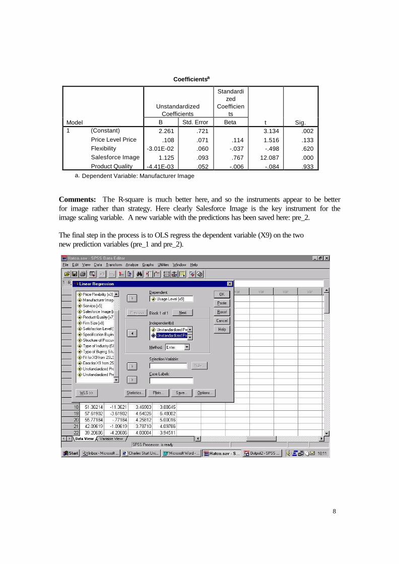
Coefficientsa

Model

Unstandardized

Coefficients

Standardi

zed

Coefficien

ts

t


1 (Constant)

Price Level Price

Flexibility

Salesforce Image

Product Quality

2.261

.108

-3.01E-02

1.125

-4.41E-03

.721

.071

.060

.093

.052

.114

-.037

.767

-.006

3.134

1.516

-.498

12.087

-.084

.002

.133

.620

.000

.933

a. Dependent Variable: Manufacturer Image

Comments: The R-square is much better here, and so the instruments appear to be better

for image rather than strategy. Here clearly Salesforce Image is the key instrument for the

image scaling variable. A new variable with the predictions has been saved here: pre_2.

The final step in the process is to OLS regress the dependent variable (X9) on the two

new prediction variables (pre_1 and pre_2).

9

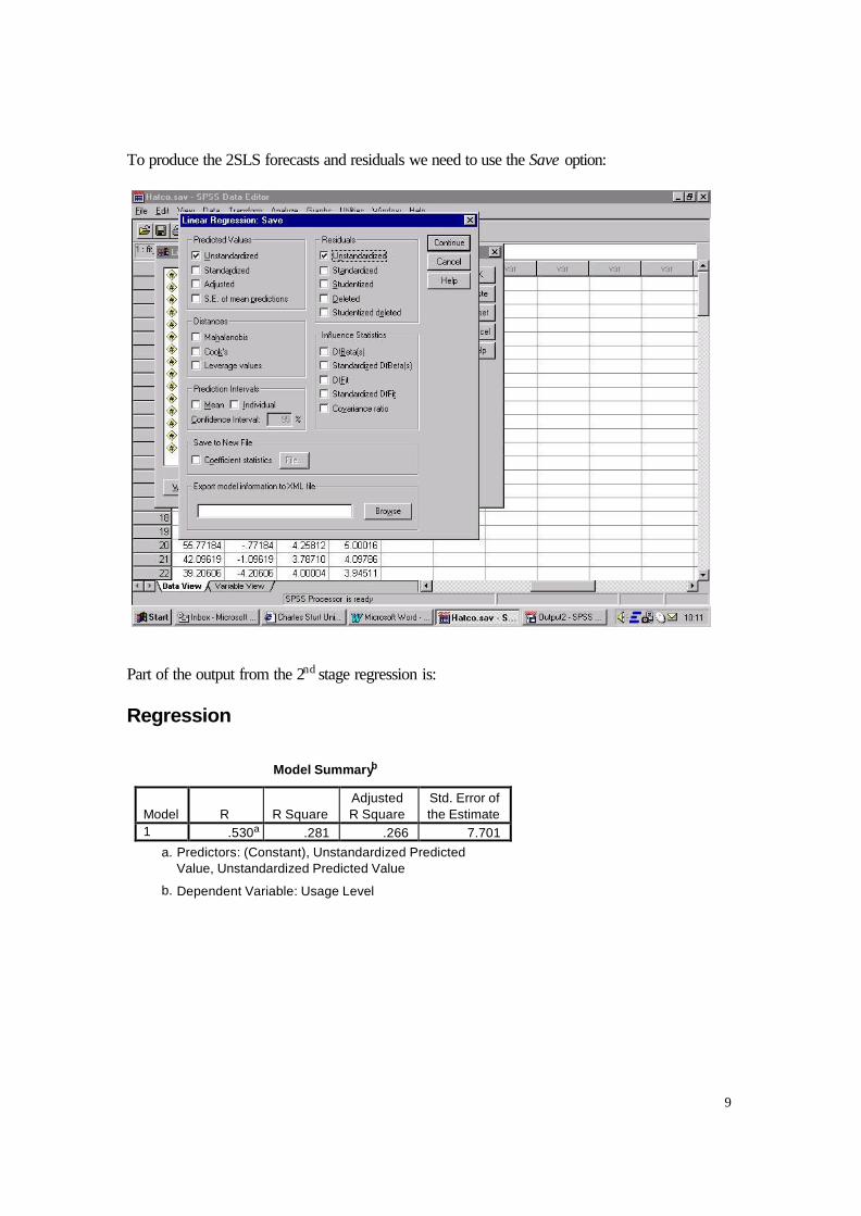
To produce the 2SLS forecasts and residuals we need to use the Save option:

Part of the output from the 2nd stage regression is:

Regression

Model Summaryb

Model

R

R Square

Adjusted

R Square

Std. Error of

the Estimate

1 .530a .281 .266 7.701

a. Predictors: (Constant), Unstandardized Predicted

Value, Unstandardized Predicted Value

b. Dependent Variable: Usage Level

10

ANOVAb

Model

Sum of

Squares

df

Mean Square

F

Sig.

1 Regression

Residual

Total

2246.200

5752.800

7999.000

2

97

99

1123.100

59.307

18.937 .000a

a. Predictors: (Constant), Unstandardized Predicted Value, Unstandardized Predicted Value

b. Dependent Variable: Usage Level

Coefficientsa

Model

Unstandardized

Coefficients

Standardi

zed

Coefficien

ts

t


1 (Constant)

Unstandardized

Predicted Value

Unstandardized

Predicted Value

15.261

5.363

2.284

5.674

.970

.856

.476

.230

2.690

5.527

2.668

.008

.000

.009

a. Dependent Variable: Usage Level

Comments: Note how the parameter estimates are the same between this regression and

the initial 2SLS model. Also note how the standard errors (and hence t and significance

levels) are different. The reported R-square is the (GR 2 ) generalized R-square referred to

in the notes and this indicates how 28.1% of the variation in the data is explained. This is

different to the initially presented R-square in the 2SLS model of 34.6%. Two new variables have been saved: pre_3 which are the 2SLS forecasts and res_1 which are the

2SLS residuals.

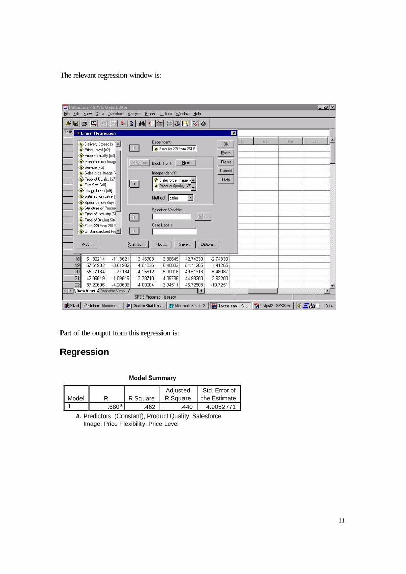
Over-identifying Restrictions Test

To perform this test we perform a regression of the IV residuals (err_1) against all the instruments: X2, X3, X6, X7. Note the R-square from this regression and multiply it by the sample size (N = 100) to get the test statistic. In this case the degrees of freedom (no. of instruments less no. of RHS variables) is (4 – 2 = 2). At the 5% level of significance

the critical value for a chi-square with d.f. = 2 is: 5.99

11

The relevant regression window is:

Part of the output from this regression is:

Regression

Model Summary

Model

R

R Square

Adjusted

R Square

Std. Error of

the Estimate

1 .680a .462 .440 4.9052771



12

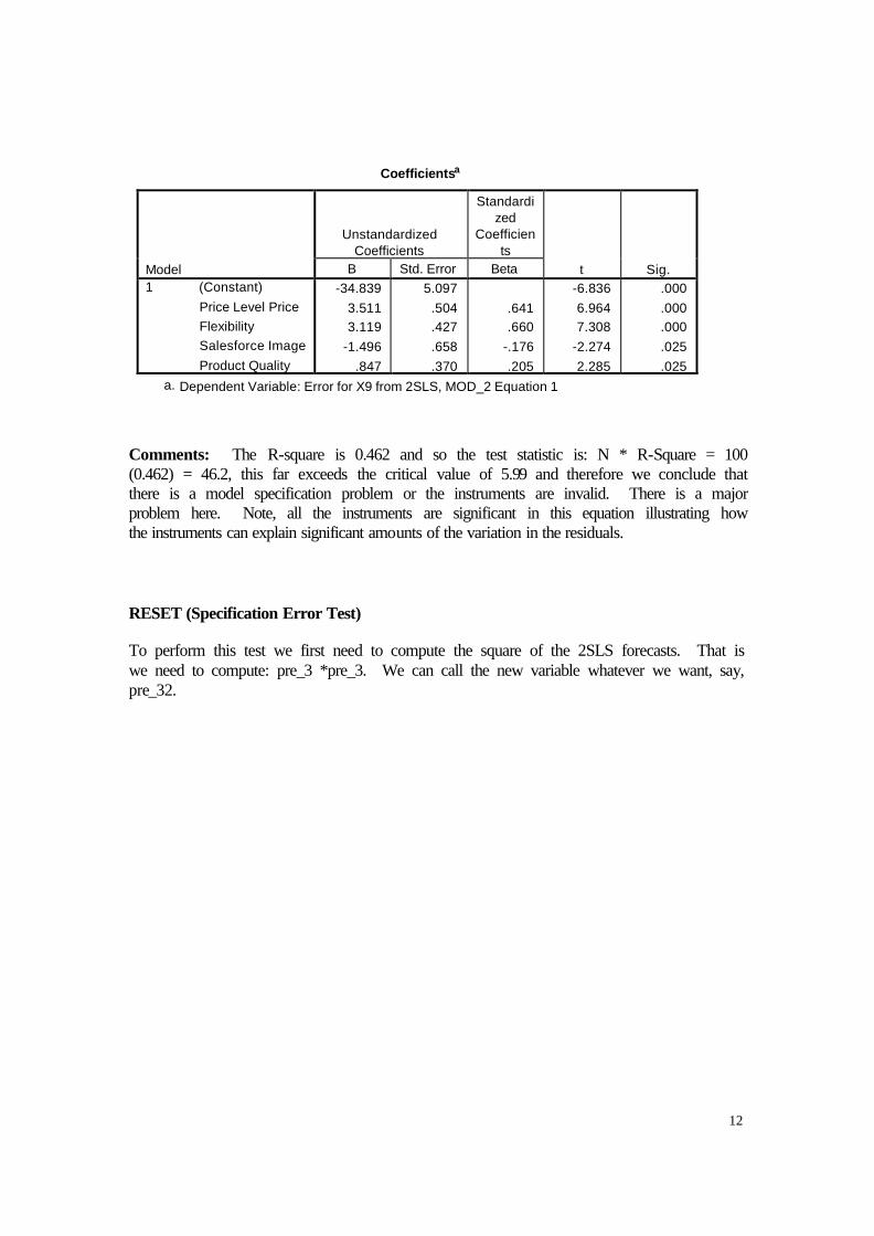
Coefficientsa

Model

Unstandardized

Coefficients

Standardi

zed

Coefficien

ts

t


1 (Constant)

Price Level Price

Flexibility

Salesforce Image

Product Quality

-34.839

3.511

3.119

-1.496

.847

5.097

.504

.427

.658

.370

.641

.660

-.176

.205

-6.836

6.964

7.308

-2.274

2.285

.000

.000

.000

.025

.025

a. Dependent Variable: Error for X9 from 2SLS, MOD_2 Equation 1

Comments: The R-square is 0.462 and so the test statistic is: N * R-Square = 100

(0.462) = 46.2, this far exceeds the critical value of 5.99 and therefore we conclude that

there is a model specification problem or the instruments are invalid. There is a major

problem here. Note, all the instruments are significant in this equation illustrating how

the instruments can explain significant amounts of the variation in the residuals.

RESET (Specification Error Test)

To perform this test we first need to compute the square of the 2SLS forecasts. That is

we need to compute: pre_3 *pre_3. We can call the new variable whatever we want, say,

pre_32.

13

To do this we use the option:

Transform � Compute

The new variable pre_32 is now added to the original 2SLS model. That is, we employ the original dependent, independent and instrumental variables, but we add to the

independent variables and instrumental variables pre_32. Part of the output from this

2SLS regression is:



Multiple R .48849

R Square .23863



14



X1

8.950208

8.336701

1.315060

1.074

.2857

X4 3.877008 3.794486 .487998 1.022 .3095

PRE_32 -.007123 .016422 -.360003 -.434 .6655

(Constant) 9.590647 14.521680 .660 .5106

Comments: The test statistic is the t-ratio for pre_32. In this case the t-ratio is –0.434

with a p-value of 0.6655. This is highly insignificant. This implies that there are no

omitted variables and the functional form can be trusted. Taken together with the

previous test, this may imply that the problems with the model relate to inadequate

instruments.

Hetero scedasticity Test

To perform this test we initially have to square the IV residuals using the compute option:

err_12 = err_1 * err_1

15

This new variable (err_12) is then regressed against the 2SLS forecasts (pre_32) and the t-ratio on the forecast variable represents the test statistic.

The output from this regression is: Regression

Model Summary

Model

R

R Square

Adjusted

R Square

Std. Error of

the Estimate

1 .069a .005 -.005 51.4851

a. Predictors: (Constant), PRE_32

16

Coefficientsa

Model

Unstandardized

Coefficients

Standardi

zed

Coefficien

ts

t


1 (Constant)

PRE_32

25.777

7.790E-03

24.997

.011

.069

1.031

.684

.305

.496

a. Dependent Variable: ERR_12

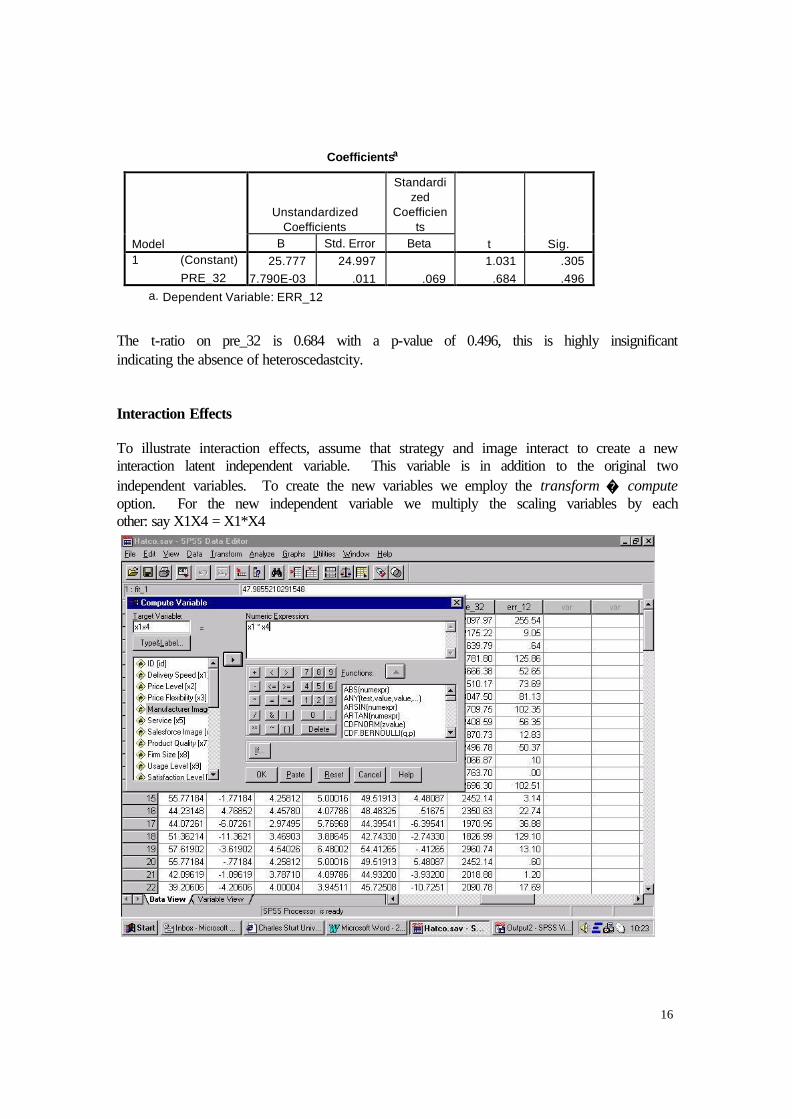
The t-ratio on pre_32 is 0.684 with a p-value of 0.496, this is highly insignificant

indicating the absence of heteroscedastcity.

Interaction Effects

To illustrate interaction effects, assume that strategy and image interact to create a new

interaction latent independent variable. This variable is in addition to the original two

independent variables. To create the new variables we employ the transform � compute

option. For the new independent variable we multiply the scaling variables by each

other: say X1X4 = X1*X4

17

The instruments for this new variable are the products of all the remaining non-scaling

variables across the two constructs. Since there is only one non-scaling variable for

image we simply multiply it with the non-scaling variables for strategy to get our

instruments:

X2X6 =X2*X6 X3X6 = X3*X6 X7X6 = X7*X6

Thus the original 2SLS model is run again with one new explanatory variable X1X4 and three new instrumental variables X2X6, X3X6, X7X6.

Part of the output from this 2SLS regression is:



Multiple R .59043

R Square .34861



18



X1

8.295013

4.662882

1.218792

1.779

.0784

X4 4.506761 3.536422 .567265 1.274 .2056 X1X4 -.555352 .859773 -.519850 -.646 .5199

(Constant) 3.577392 19.010684 .188 .8511

Comments: Note, this model appears to be inferior to the original specification. All the variables are now insignificant, including the new interaction term X1X4.

Non-nested Testing

To illustrate these tests consider two models:

Model A: Usage Strategy

Model B: Usage Image

Assume we wish to ascertain which variable better explains usage. We will conduct a

paired test alternating the role of Models A and B.

Case 1

H0: Null model: Usage Strategy

H1: Alternative model: Usage Image

In terms of our notation, our x’s are the strategy indicators while the w’s are the image indicators. The three steps are:

1. Regression: X4 on X6 and save the predictions (pre_4).

2. 2SLS regression X9 on X1 and pre_4 (instruments: X2, X3, X7 and pre_4). 3. The t-ratio on the pre_4 variable is the test statistic.

The output from this 2SLS regression is:



Multiple R .58664

R Square .34415



19



X1

5.095873

.822486

.748740

6.196

.0000

PRE_4 1.998917 .735642 .198320 2.717 .0078

(Constant) 17.697687 4.564165 3.878 .0002

Comments: The t-ratio for Pre_4 is 2.717 with a p-value of 0.0078, this is highly

significant. This implies that the alternative model H1 image rejects the null model H0

strategy.

Case 2

H0: Null model: Usage Image

H1: Alternative model: Usage Strategy

In terms of our notation our, x’s are the image indicators while the w’s are the strategy

indicators. The three steps are:

1. Regression: X1 on X2,X3,X7 and save the predictions (pre_5).

4. 2SLS regression X9 on X4 and pre_5 (instruments: X6 and pre_5).

5. The t-ratio on the pre_5 variable is the test statistic.

The output from this 2SLS regression is:

Two-stage Least Squares Dependent variable.. X9

Multiple R .53666

R Square .28800





X4

3.227772

.886499

.406279

3.641

.0004

PRE_5 6.010515 1.032240 .515718 5.823 .0000

(Constant) 8.033696 6.596728 1.218 .2262

Comments: The t-ratio for Pre_5 is 5.823 with a p-value of 0.0000, this is highly

significant. This implies that the alternative model H1 strategy rejects the null model H0

image.

In summary these results combined imply that both models reject each other and

therefore it is erroneous to use either in isolation.

20

2SLS HATCO STATA EXAMPLE

This section presents the STATA code corresponding to the SPSS example.

* Original 2SLS model

ivregress 2sls X9 (X1 X4 = X2 X3 X7 X6)

predict FIT_1

predict ERR_1, r

* 2 step OLS version to get 2SLS predictions, residuals and GR^2

regress X1 X2 X3 X6 X7

predict PRE_1

regress X4 X2 X3 X6 X7

predict PRE_2

regress X9 PRE_1 PRE_2

predict PRE_3

predict RES_1, r

* Over-identifying restrictions test

regress ERR_1 X2 X3 X6 X7

gen OIR=e(N)*e(r2)

display OIR

*RESET test

gen PRE_32=PRE_3*PRE_3

ivregress 2sls X9 PRE_32 (X1 X4 = X2 X3 X7 X6 PRE_32)

* Heteroscedasticity Test

gen ERR_12=ERR_1*ERR_1

regress ERR_12 PRE_32

* Interactions Model Specification

gen X1X4=X1*X4

gen X2X6=X2*X6

gen X3X6=X3*X6

gen X7X6=X7*X6

ivregress 2sls X9 (X1 X4 X1X4 = X2 X3 X7 X6 X2X6 X3X6 X7X6)

* Non-nested Test Case 1

regress X4 X6

predict PRE_4

ivregress 2sls X9 PRE_4 (X1 = X2 X3 X7 PRE_4)


regress X1 X2 X3 X7

predict PRE_5

ivregress 2sls X9 PRE_5 (X4 = PRE_5 X6 PRE_5)

21

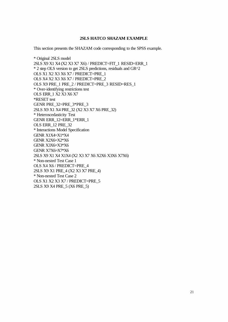
2SLS HATCO SHAZAM EXAMPLE

This section presents the SHAZAM code corresponding to the SPSS example.

* Original 2SLS model

2SLS X9 X1 X4 (X2 X3 X7 X6) / PREDICT=FIT_1 RESID=ERR_1 * 2 step OLS version to get 2SLS predictions, residuals and GR^2

OLS X1 X2 X3 X6 X7 / PREDICT=PRE_1 OLS X4 X2 X3 X6 X7 / PREDICT=PRE_2

OLS X9 PRE_1 PRE_2 / PREDICT=PRE_3 RESID=RES_1

* Over-identifying restrictions test OLS ERR_1 X2 X3 X6 X7

*RESET test GENR PRE_32=PRE_3*PRE_3

2SLS X9 X1 X4 PRE_32 (X2 X3 X7 X6 PRE_32) * Heteroscedasticity Test

GENR ERR_12=ERR_1*ERR_1

OLS ERR_12 PRE_32 * Interactions Model Specification

GENR X1X4=X1*X4 GENR X2X6=X2*X6

GENR X3X6=X3*X6

GENR X7X6=X7*X6

2SLS X9 X1 X4 X1X4 (X2 X3 X7 X6 X2X6 X3X6 X7X6)

* Non-nested Test Case 1 OLS X4 X6 / PREDICT=PRE_4

2SLS X9 X1 PRE_4 (X2 X3 X7 PRE_4)


OLS X1 X2 X3 X7 / PREDICT=PRE_5

2SLS X9 X4 PRE_5 (X6 PRE_5)

2SLS HATCO SPSS, STATA and SHAZAM Example by Eddie Oczkowski August...

Documents

Transcript of 2SLS HATCO SPSS, STATA and SHAZAM Example by Eddie Oczkowski August...