1

ShaDe for SketchUp©

User's Guide All rights reserved

For research use only (non-commercial use) © Manuela Ruiz Montiel and Universidad de Málaga

Author Manuela Ruiz Montiel

Date September 5, 2012

Version of ShaDe 2.4

2

Contents 0. Introduction ......................................................................................................... 4

1. SketchUp canvas and basic tools ........................................................................... 6

2. Installing the plugin .............................................................................................. 9

3. Basic functionality of ShaDe ................................................................................ 10

3.1 New project ......................................................................................................... 11

3.2 Open project ........................................................................................................ 11

3.3 Save project (as) ................................................................................................... 11

3.4 New grammar ....................................................................................................... 12

3.5 Open grammar ...................................................................................................... 12

3.6 Save grammar as .................................................................................................. 12

3.6 Add rule ................................................................................................................ 13

3.7 Delete rule ............................................................................................................ 13

3.8 Copy rule ............................................................................................................... 13

3.9 Rules edition ......................................................................................................... 13

3.9.1 Loading new shapes ...................................................................................... 14

3.9.2 Transforming shapes ..................................................................................... 15

3.9.3 Saving shapes ................................................................................................. 18

3.10 Specifying the source of the axiom .................................................................... 18

3.11 Applying a rule .................................................................................................... 18

3.12 Apply a random rule ........................................................................................... 19

3.13 Apply a number of random rules ....................................................................... 19

3.14 Undo a step ......................................................................................................... 19

3.15 Reset design ........................................................................................................ 19

3.16 Save design ......................................................................................................... 19

3.17 Show labels ......................................................................................................... 19

3.18 Hide labels .......................................................................................................... 19

3.19 Change the radius of labels ................................................................................ 20 3.20 Convert to 3D shape ........................................................................................... 19

3.18 Convert to 2D shape ........................................................................................... 20

4. Layers ................................................................................................................. 22

5. Constraints and goals .......................................................................................... 25

5.1 Add a constraint ................................................................................................... 25

5.2 Add a custom constraint ....................................................................................... 25

5.3 Remove a constraint ............................................................................................. 35

5.4 View project constraints ....................................................................................... 35

5.6 Add a goal ............................................................................................................. 35

5.7 Add a custom goal ................................................................................................ 35

5.8 Remove a goal ...................................................................................................... 36

5.9 View project goals ................................................................................................ 36

5.10 Verify goals ......................................................................................................... 36

5.11 Apply rules until the goals are satisfied.............................................................. 36

6. Design scripts ..................................................................................................... 38

6.1 Create a script ....................................................................................................... 38

6.2 Execute a script ..................................................................................................... 39

3

6.3 Load a script .......................................................................................................... 39

7. Frequent problems ............................................................................................. 40

4

0. Introduction Google SketchUp is a 3D modelling software that combines a tool-set with an intelligent drawing system. Along with its Ruby API, it can be extended and customized to satisfy particular and concrete needs that may go from automation of common tasks to the creation of personal drawing tools. This is managed through the creation of Ruby scripts that will work as Sketchup plugins. ShaDe for Sketchup is one of them. The aim of this plugin is to offer the user a way of creating, editing and experimenting 2D shape grammars. A shape grammar is a formalism that represents visual thinking. The proceeding way is the application of visual rules like the one in figure 1 to a given design. A grammar is a set of this kind of rules plus an initial design (a shape) called axiom.

Figure 1: A rule

These rules tell: "see the left side in a design and replace it with what is on the right". As we have said, the initial design is the axiom, and we start applying the rules from it, trying to match some sub-shape in the design with the left part of some rule. Then, we would replace the matched shape with what is on the right part of the rule, always applying to it the same transformation that we did in order to match the left shape. In figure 2 we can see an example of rule derivation, starting from a square as axiom:

Figure 2: A rule derivation

Our plugin will allow the creation and edition of 2D design grammars and the application of its rules to a design. The user will be able to configure the rules and see how the design changes as the rules are edited. The plugin will also allow the imposition of custom constraints and goals to the derivation process, in order to control the global composition of the designs.

5

This user guide contains some special sections:

These squares contain pieces of information that can be useful or deserve special attention.

These squares contain very important information that has to be considered when working with ShaDe for SketchUp.

6

1. SketchUp canvas and basic tools Before explaining the plugin itself, it may be necessary to have a brief look at the main features of SketchUp canvas and basic tools, which manipulation is needed to use the 2D Shape Grammars Tool.

Screenshot 1: Google SketchUp

In screenshot 1 we can see the canvas and a toolbar with some basic tools. The recommended template is the one that takes the units as meters and puts the camera at the top, thus we can see a 2D space. Selecting Window -> Preferences -> Templates, the dialog for changing our template will appear (screenshot 2).

Screenshot 2: Choosing template

7

In order to move the canvas we should use the hand tool. The selection tool selects anything in the canvas. In our plugin, the rule shapes will be groups. In Google SketchUp, a group is a set of lines, faces and possibly other groups that go together. That is, one cannot change the relative position between the lines, faces and internal groups; so a square, for example, will always be a square -and not a rectangle or a rhombus, unless we enter the group. Thus, to modify the groups, we need to enter them. By double-clicking a shape, its group will be opened and then we will be able to do modifications such translations, rotations and scales or even adding or removing units.

Allowed modifications can be performed by the use of three tools:

Move/Rotate tool : The same tool can be used either to move or rotate a shape in the canvas. When placing the cursor over the red crosses (if present, in case the shape is a group), it becomes a rotator.

Screenshot 4: Moving

Screenshot 5: Rotation

Screenshot 3: Inside a group

8

Scale tool : This one is used to scale a shape. The plugin will only allow uniform scales.

Screenshot 6: Scaling

Rotate tool : This one is used to rotate a shape.

Screenshot 7: Rotating a shape with the rotate tool

We can use these tools in order to transform the main groups without entering them, and also the entities inside the groups. In section 3.9 we will further explain the shape and rule edition. Moreover, we can use the paint tools of SketchUp for drawing inside the groups. These tools are the following:

Pencil tool : For drawing lines

Square tool : For drawing squares

Circle tool : For drawing circles

Arc tool : For drawing arcs

9

2. Installing the plugin To run the plugin, at least Google SketchUp 8 is needed. Once it is installed, the extension scripts (shade_extension.rb) and the code folder (Shade) must be copied into the SketchUp Plugins directory. If any previous version has been installed, erasing the associate files is crucial for the proper running of the plugin.

10

3. Basic functionality of ShaDe The first time we launch SketchUp after copying the files into the Plugins directory, we need to select Window -> Preferences -> Extensions and activate ShaDe. Now, we can launch the plugin by selecting Plugins > ShaDe. The next time we open SketchUp, the activation step will not be necessary, that is, we will see the plugin option beneath the Plugins tab directly. Once the plugin has been launched, several changes are going to take place:

The xyz axis have disappeared

The canvas is filled with a default project

Three new toolbars have appeared (two for execution and one for edition tasks).

We can see them in screenshot 8.

Screenshot 8: Default view of the plugin

We can re-shape the toolbars and place them wherever we want, even fitting them into the SketchUp reserved places for toolbars. Inside the canvas, we can see two different areas. The right one is reserved for the generated design, and at the beginning, it only has one shape: the axiom. The left part contains the rules that set up the grammar -at the moment there is only one.

11

The shapes which we are going to work with are represented as sets of edges and points. These points can be of two kinds: intersection points, that is, points where two or more edges coincide, and label points, that is, points with an associated mark. The default shapes are an unlabelled square for the left part of the rule and two overlapped unlabelled squares for the right part of the rule. The axiom is, by default, the left shape of the first rule (the square in this case), but, as we will see later, it can be loaded from a SketchUp file. In the next sections we will go through the offered functionalities.

3.1 New project

Whenever the user wants, he or she can start a new, default project, that is, the one that we can see in screenshot 9. A prompt will appear in case the previous project is not saved. What do we understand for project? Our project is the union of a grammar and a set of constraints and goals. Constraints and goals will be further explained in next sections. By the moment we can say that they determine the execution of the grammar, analysing the generated design in each step.

3.2 Open project

This option will open a previously saved project. A prompt will appear in case the previous project is not saved.

3.3 Save project (as)

When the user is happy with the configured project, it can be saved to a .prj file and thus be opened later.

Please note that there is a cross in the origin of every rule shape. This symbol is not part of the shape, and it is only present for establishing the spatial relation between the left and the right part of each rule.

12

3.4 New grammar

If we need to reset the grammar of our project, with this option a default one will be loaded. A prompt will appear in case the current project is not saved, just to ask if the current grammar needs to be saved for future use.

3.5 Open grammar

If we need to load a grammar in our project, with this option a default one will be loaded. A prompt will appear in case the current project is not saved, just to ask if the current grammar needs to be saved for future use.

3.6 Save grammar as

If we want to have the current grammar as a separate file, in order to re-use it in further projects, we can have it saved with this option, as a .gr2 file.

Screenshot 10: Project files. They need to be in the same directory.

When saving grammars and project, apart from the .prj or .gr2 files, the plugin will generate a .txt file for every rule shape. Moreover, if the axiom has been loaded from a file, the plugin will also generate a .txt file with the axiom specification. These files are necessary for loading the grammars and projects in the future, and the application searches for them in the same directory where the .prj or .gr2 file is. In the same way, when saving a project, a .gr2 file will be saved in the same directory, representing its grammar.

Screenshot 9: Necessary files for a project

13

3.6 Add rule

We can add more rules to the grammar. The added rule will be appended at the end of the rule list, and its appearance will be like the one of the rule in screenshot 8 -the default rule. In screenshot 10 we can see new rules (rule 2 and rule 3). We can add any number of rules.

3.7 Delete rule

Any rule can be deleted, except if there is only one rule. If the axiom (rule 1) is deleted, and the axiom has not been loaded from a file, then the new axiom will be the left shape of rule 2, which now is going to be the new rule 1.

3.8 Copy rule

In case we want to add a rule that is similar to some existing rule, then we can copy it in order to further edit it. A prompt in which we have to enter the rule-to-copy index will appear, and the new rule will be added to the end of the list.

Screenshot 110: Rule 2 and rule 3 added

3.9 Rules edition

There are two main ways of editing a rule: changing the whole shapes or transforming them. When changing rules, the current design will not be affected until a new execution of the grammar is performed.

14

3.9.1 Loading new shapes

We can load a previously saved shape (in .txt format) into a rule part with the

command . A sample shape file would be:

That is, we specify the segments with a capital letter ‘S’ and labels with a capital ‘L’, and then just provide two 2D points, in the case of segments, or one, in the case of labels. In this last case it is also necessary to write the colour of the label. The unit of measure is the meter.

The allowed colors that can appear in the text files are the following: "AliceBlue", "AntiqueWhite", "Aqua", "Aquamarine", "Azure", "Beige", "Bisque", "Black", "BlanchedAlmond", "Blue", "BlueViolet", "Brown", "BurlyWood", "CadetBlue", "Chartreuse", "Chocolate", "Coral", "CornflowerBlue", "Cornsilk", "Crimson", "Cyan", "DarkBlue", "DarkCyan", "DarkGoldenrod", "DarkGray", "DarkGreen", "DarkKhaki", "DarkMagenta", "DarkOliveGreen", "DarkOrange", "DarkOrchid", "DarkRed", "DarkSalmon", "DarkSeaGreen", "DarkSlateBlue", "DarkSlateGray", "DarkTurquoise", "DarkViolet", "DeepPink", "DeepSkyBlue", "DimGray", "DodgerBlue", "FireBrick", "FloralWhite", "ForestGreen", "Fuchsia", "Gainsboro", "GhostWhite", "Gold", "Goldenrod", "Gray", "Green", "GreenYellow", "Honeydew", "HotPink", "IndianRed", "Indigo", "Ivory", "Khaki", "Lavender", "LavenderBlush", "LawnGreen", "LemonChiffon", "LightBlue", "LightCoral", "LightCyan", "LightGoldenrodYellow", "LightGreen", "LightGrey", "LightPink", "LightSalmon", "LightSeaGreen", "LightSkyBlue", "LightSlateGray", "LightSteelBlue", "LightYellow", "Lime", "LimeGreen", "Linen", "Magenta", "Maroon", "MediumAquamarine", "MediumBlue", "MediumOrchid", "MediumPurple", "MediumSeaGreen", "MediumSlateBlue", "MediumSpringGreen", "MediumTurquoise", "MediumVioletRed", "MidnightBlue", "MintCream", "MistyRose", "Moccasin", "NavajoWhite", "Navy", "OldLace", "Olive", "OliveDrab", "Orange", "OrangeRed", "Orchid", "PaleGoldenrod", "PaleGreen", "PaleTurquoise", "PaleVioletRed", "PapayaWhip", "PeachPuff", "Peru", "Pink", "Plum", "PowderBlue", "Purple", "Red", "RosyBrown", "RoyalBlue", "SaddleBrown", "Salmon", "SandyBrown", "SeaGreen", "Seashell", "Sienna", "Silver", "SkyBlue", "SlateBlue", "SlateGray", "Snow", "SpringGreen", "SteelBlue", "Tan", "Teal", "Thistle", "Tomato", "Turquoise", "Violet", "Wheat", "White", "WhiteSmoke", "Yellow", "YellowGreen" In order to check how they look like, please visit: http://en.wikipedia.org/wiki/X11_color_names

15

In section 3.9.3 we can see the command for saving shapes. If we want to copy a rule shape into another part of any rule, we can manage it through this command. We can choose the origin and destiny shapes (screenshot 11).

Screenshot 121: Copy shape dialog

If a shape has been removed and we need to draw it again, then we should use the command in order to re-introduce the corresponding SketchUp group. This command will draw the default left or right shape, depending on the affected part of the rule. The default left part is a square and the default right one is a group of two overlapping squares.

3.9.2 Transforming shapes

Using the tools mentioned in section 1, we can edit the rule shapes. We have three options:

1. Transforming the groups as a whole. We can use the transforming (move, rotate and scale) tools. If we use the painting tools outside the groups, the new lines are not registered as part of the shapes and it will have no effect in the grammar execution.

Some important considerations regarding the format of the text files for shapes:

Its extension must be .txt The letters S and L must be capitals, and they must be followed by two dots (:) For segments we must specify two points (that is, the start and the end of the

segment), so we need to provide four numbers separated by at least one space For labels we must specify one point (that is, two numbers separated by at least one

space) and its color If some of the previous considerations is violated, then an error message will appear

when loading the file The unit of measure is the meter

16

2. Entering the groups. Inside a group we can use both the transforming and painting (line, square, circle and arc) tools. Everything we paint inside a group is considered in the execution.

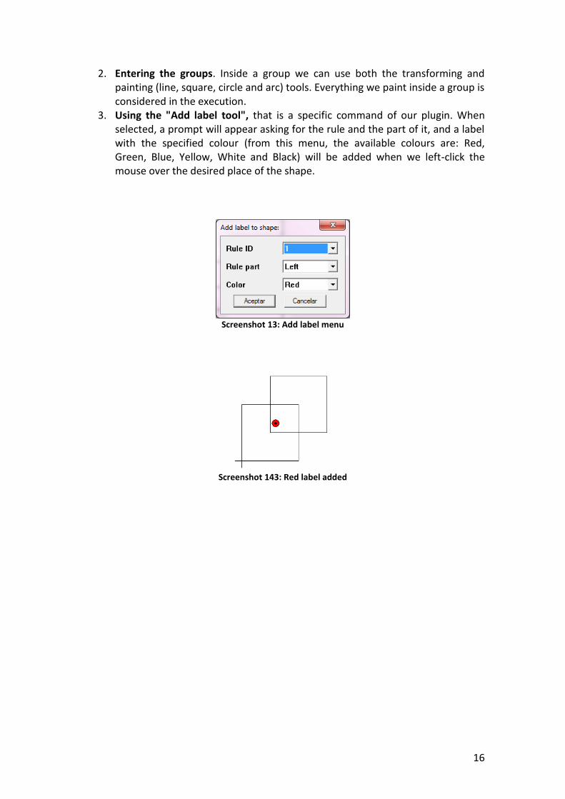
3. Using the "Add label tool", that is a specific command of our plugin. When selected, a prompt will appear asking for the rule and the part of it, and a label with the specified colour (from this menu, the available colours are: Red, Green, Blue, Yellow, White and Black) will be added when we left-click the mouse over the desired place of the shape.

Screenshot 13: Add label menu

Screenshot 143: Red label added

17

Be careful when choosing the rule part for adding a label. Placing the cursor over a shape does not mean that the label will be added to it: it will be always added to the rule part that was specified in the menu depicted in screenshot 12. For example, if we add a label to the left part, as determined in screenshot 12, and then place the cursor over the right part, the label will still be joined to the left one:

Sometimes, when adding segments, SketchUp adds automatically some faces to the shapes, with the default material:

This faces do not affect the execution of the grammar, but we can easily remove them by using the selection tool and then right-clicking and pressing “Erase” or just pressing “Supr”:

18

3.9.3 Saving shapes

We can save a rule shape into a .txt file with this button. A prompt will appear, asking which shape is to be saved, specifying the rule and the part of it.

3.10 Specifying the source of the axiom

With the first button, we can load an axiom from a .txt file. With the second one, we specify that the axiom is the left part of the first rule.

3.11 Applying a rule

We can make our grammar run by applying rules to the design. When we choose this option, a prompt will appear. It will ask us to choose the rule to apply, by its position in the list. It will be applied only if its left shape is a subshape of the current design, by means of a transformation. Every time a rule is applied, an execution history is updated with a pair that stores, among other things, the applied rule and the

If we still want to use the editing tools of SketchUp to edit the current shape, then we can use the next procedure:

1. Save the left part of the first rule into a .txt file 2. Save the current shape into a .txt file with the command explained in section 3.16 3. Load the file produced in (2) into the left part of the first rule 4. Perform the desired editions 5. Now we can choose between:

a. Save the left part again into another text file and load it into the axiom b. Specify that the axiom is the left part of the first rule

6. Now, restore the left part of the first rule by loading the file produced in (1)

The axiom, and in general the produced shape at the right part of the canvas, should not be edited by hand from the plugin, because it is supposed to be generated exclusively by the shape grammar. Actually it can be edited, but the performed changes will not be registered in the internal representation of the shape. If we need to change the axiom or the current shape, we can use one of the two tools explained above.

Sometimes it can be difficult to add labels or paint segments with certain precision. We recommend working with text files when possible, or getting familiarized with the SketchUp hints for getting accuracy: http://youtu.be/DVO1cpDLbrs. You can also find a video tutorial for some ShaDe tasks in http://youtu.be/VgUyjurOlUQ. Being precise is of crucial importance when working with ShaDe if we want the subshape matching algorithm to work as we expect.

19

transformation that was performed in order to make the left part of the rule a subshape of the current design.

3.12 Apply a random rule

Sometimes there is more than one fitting rule for a given shape. Moreover, we can randomly choose both the rule and subshape to be affected in the next step. That is the aim of this command. In case it is impossible to apply any rule to any shape of the design, then a message will appear. Now we can press this button many times and see how a random design appears.

3.13 Apply a number of random rules

In case we want to apply certain number of random rules at once, we can use this command. The application of a large number of rules can be somewhat slow (we use a backtracking process). We can see the steps that are being applied during this time.

3.14 Undo a step

We can remove the last step by clicking this button.

3.15 Reset design

At any moment, we can reset the design, so the shape in it is the axiom.

3.16 Save design

In case the generated design is worthy, it can be saved to a .txt file.

3.17 Show labels

In order to see the labels in the current shape, we can use this command.

3.18 Hide labels

In order to hide the labels in the current shape, we can use this command.

When any of the commands in sections 3.11, 3.12 and 3.13 is used, the plugin will use an external command for execute them, so as to speed up the rule application process (the Ruby interpreter that comes along with SketchUp can become a bit slow). A shell will appear during the execution process, then it will disappear and the produced shape will be shown in the right part of the canvas.

20

3.19 Change the radius of labels

We can specify the radius of the labels with this command.

3.20 Convert to 3D shape

With this command, we can convert to 3D the current shape. For each layer, the user must indicate two values of the z component per layer, z and z’ (Figure 3).

Figure 3

When this button is pressed, we will be able to choose if we want to introduce the values for each layer or open the values from a file (Screenshot 14).

Screenshot 14: Convert to 3D shape dialogue

On the one hand, if we have chosen Open the 3D values from a file, the file must contain two numbers per layer; otherwise, the file will not be able to be used. On the other hand, if we have chosen Introduce the 3D values, a window will appear and we must introduce, again, two numbers per layer(Screenshot 15). aaa

21

ff

Screenshot 15: Introduce the 3D values window

aaa

3.21 Convert to 2D shape

If we have a 3D current shape, we can convert to 2D shape using this button.

When we load a file which was saved like a 3D format and we press the 3D button, the program does not ask us, it loads the z values which were specified in the file. The 3D text file must contain in the first line the word 3D: and the z values. Example: 3D: 5.0 6.0

22

4. Layers

We can take advantage of the layer system of SketchUp in order to edit layered grammars. To see the layers window, open the menu ‘Window’ and choose ‘Layers’. The small window shown in screenshot 16 will appear.

Screenshot 16: Layers Window

To add a layer, click the top-left button ‘+’ inside this window. After typing a name and activating the new layer by selecting its associated radio-button, now our initial shape grammar will have two layers. The policy for filling the new added layers is to copy inside them the content of the first existing non-empty layer in the current grammar. In order to explain the process of editing the grammar and executing it when multiple layers are present, we provide the following step-by-step example, starting from the default shape grammar: 1. Add a layer and type in the name: “Layer1”. 2. Click the radio-button associated with the new added layer. 3. Make Layer1 visible and Layer0 invisible. Check that both layers are identical, since Layer1 has been filled with a copy of the content of Layer0.

4. Edit the Layer1 of the right shape of the rule, adding a diagonal in one of the squares.

23

5. Apply a rule using the command. The rule can be applied since the axiom has a square in both layers, and thus the left part of the rule, which also has a square per layer, is a sub-shape of the axiom. That is, for a rule to be applied, its left shape must be a sub-shape of the current shape, regarding all its layers. Now we can see how the rule has been applied by making visible only Layer1 or only Layer0. When only Layer1 is visible, we can see the diagonal in the current shape:

But in the case of Layer0, we can only see two squares:

The format of the text files for storing the layered shapes is the same as shown in section 3.9.1. If we load files such as the one provided there, then all the segments and labels will be stored inside Layer0, which is the default layer in SketchUp. But if the shape has entities among several layers, then we have to specify which segments and labels go in which layers:

24

LAYER: Layer0 S: 0.0 0.0 8.0 0.0 S: 4.0 4.0 12.0 4.0 S: 0.0 8.0 8.0 8.0 S: 4.0 12.0 12.0 12.0 S: 0.0 0.0 0.0 8.0 S: 4.0 4.0 4.0 12.0 S: 8.0 0.0 8.0 8.0 S: 12.0 4.0 12.0 12.0 LAYER: Layer1 S: 4.0 12.0 12.0 4.0 S: 0.0 0.0 8.0 0.0 S: 4.0 4.0 12.0 4.0 S: 0.0 8.0 8.0 8.0 S: 4.0 12.0 12.0 12.0 S: 0.0 0.0 0.0 8.0 S: 4.0 4.0 4.0 12.0 S: 8.0 0.0 8.0 8.0 S: 12.0 4.0 12.0 12.0

25

5. Constraints and goals

5.1 Add a constraint

We have the option of imposing constraints on the generated design. This means that each time a new design is generated, the plugin will check if these constraints are complied. In case that one of them is not complied, then the application of the last rule will be undone.

In case of the command , when a constraint is broken, a message appears. Nevertheless, if we are using the random commands (those with the '?' mark), the plugin will try another rule. If the algorithm runs out of alternatives, then a message will appear, saying that is impossible to complete the process. Some pre-programmed constraints are available:

Produce Distinct Shape constraint: This ensures that the application of a rule always changes the design.

No Scales constraint: The algorithm of sub-shape recognition will not take into account scale transformations.

Area constraint: The design is always inside a given area, that can be specified in a text file of points. For example:

50 -50 0 50 7.3 0 200 7.3 0 200 -50 0

5.2 Add a custom constraint

Apart from the pre-programmed constraints, the users are able to program their own constraints and having them stored in order to use them in following work sessions with the plugin. This can be managed by two alternatives interfaces:

1. A CODE interface that allows directly writing, syntax-checking and executing custom Ruby code (screenshot 17):

26

Screenshot 167: Interface for adding custom constraints

Once the ‘ok’ button is pressed, the new constraint is added to the project, and also it will be available for adding it with the command in future work sessions with the plugin, stored inside the directory ‘custom_constraints’ as a .txt file. Within this interface, two potentially useful links are provided: one for the SketchUp API documentation (in case some function of the SketchUp API is necessary) and another one for the ShaDe software documentation, which is provided in HTML format along with the plugin files.

2. A graphic (GUI) interface that allows the addition of custom constraints with the help of a wizard. The first step one the GUI interface has been chosen is the one depicted in screenshot 18.

27

Screenshot 178: Choosing main focus of a constraint

The aim of this step is choosing the main focus of a constraint. We can have two different focuses: we can impose constraints over the rule that has been applied and, on the other hand, to the shape that is produced. We first illustrate the rule focus:

Screenshot 19: Choosing rule focus

When imposing a constraint to the applied rule, we may refer to several aspects: (1) the ID of the rule being applied (RULE ID), (2) the transformation of the rule being applied (TRANSFORMATION) and (3) a special case that only takes into account the ID of the first rule applied (FIRST RULE APPLIED). This last case is useful if the user wants to specify which rule is to be applied in first place. The RULE ID constraint is configured by the screen depicted in screenshot 20.

Screenshot 20: Configuring the RULE ID constraint

The possibilities are specified in two lists (1 and 2) and one text box (3). The list (1) gathers all the possibilities depicted in screenshot 21.

Screenshot 21: Configuring the RULE ID constraint (II)

The list (2) gathers two possibilities, as shown in screenshot 22.

28

Screenshot 182: Configuring the RULE ID constraint (III)

In case the first option (“the previous rule ID) of screenshot 20 is chosen, then the configuration is done. When the “number” option is chosen instead, we still need to write a number in the text field (3). For example, for editing the constraint: “the rule applied must be always the following to the previous one”, the configuration must be the one depicted in screenshot 23. In this case, the content of the text field (3) will be ignored.

Screenshot 193: Constraint: the applied rule must be always following to the previous one

The TRANSFORMATION constraint of screenshot 17 is configured by means of the screen depicted in screenshot 24.

Screenshot 204: Configuring the TRANSFORMATION constraint

The list (1) gathers some aspects of the applied transformation that the constraint may refer to. We can see these aspects in screenshot 25.

Screenshot 215: Configuring the TRANSFORMATION constraint (II)

That is, we can impose constraints over the traslation, rotation and scale of the applied transformation, by means of the comparators in the list (2) (see screenshot 26)

29

Screenshot 226: Configuring the TRANSFORMATION constraint (III)

For example, if we want to forbid scales bigger than 2x factor (that is, that add the right part of the involved rule more than twice as bigger), we should configure the options as in screenshot 27.

Screenshot 237: Constraints: forbid those transformations that involve scales with factor

bigger than 2x (in the x-axis)

The FIRST RULE APPLIED constraint of screenshot 20 is configured by means of the screen depicted in screenshot 28.

Screenshot 248: Configuring the FIRST RULE APPLIED constraint

In this case, we only have to specify the comparator in the list and a number in the text field. If we choose the focus CURRENT SHAPE of screenshot 19, we obtain the screen depicted in screenshot 29.

Screenshot 29: Choosing current shape focus

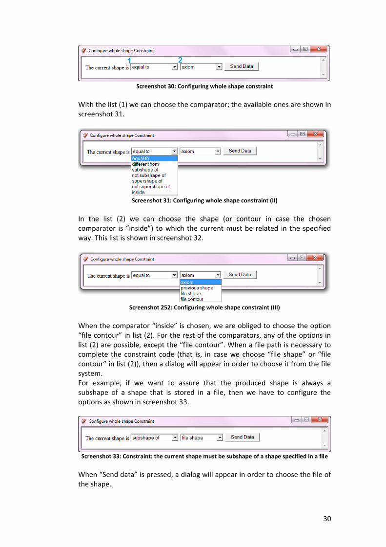
With the focus WHOLE SHAPE we can configure constraints that affect the shape as a whole, in the sense that it must, for example, be subshape of other shape or be inside certain contour. This kind of constraints can be configured by means of the screen depicted in screenshot 30.

30

Screenshot 30: Configuring whole shape constraint

With the list (1) we can choose the comparator; the available ones are shown in screenshot 31.

Screenshot 31: Configuring whole shape constraint (II)

In the list (2) we can choose the shape (or contour in case the chosen comparator is “inside”) to which the current must be related in the specified way. This list is shown in screenshot 32.

Screenshot 252: Configuring whole shape constraint (III)

When the comparator “inside” is chosen, we are obliged to choose the option “file contour” in list (2). For the rest of the comparators, any of the options in list (2) are possible, except the “file contour”. When a file path is necessary to complete the constraint code (that is, in case we choose “file shape” or “file contour” in list (2)), then a dialog will appear in order to choose it from the file system. For example, if we want to assure that the produced shape is always a subshape of a shape that is stored in a file, then we have to configure the options as shown in screenshot 33.

Screenshot 33: Constraint: the current shape must be subshape of a shape specified in a file

When “Send data” is pressed, a dialog will appear in order to choose the file of the shape.

31

When the focus POINTS of screenshot 29 is chosen, we obtain the screen depicted in screenshot 34. This focus must be chosen when the constraint refers to the points (that is, intersections or labels) of the shape.

Screenshot 34: Choosing constraint points focus

Again, we need to choose between two options. When our constraint is related to the amount of points of the current shape, we choose the option NUMBER OF POINTS. The screen shown in screenshot 35 will appear.

Screenshot 265: Configuring number of points constraint

The list (1) gathers some types of points that can be found inside a shape (screenshot 36). We must choose the type we are referring to; for example, if we want to impose some constraint about the existing blue labels in the current shape, then we need to choose the option “blue”.

Screenshot 276: Configuring number of points constraint (II)

With the second list we can establish the comparator of the constraint (screenshot 37).

32

Screenshot 37: Configuring number of points constraint (III)

Now, if we let the list in (3) with the option “number”, as seen in screenshot 35, we just need to write a number inside the text field (4), and our constraint will assure that the current shape has always a certain number of blue labels (screenshot 38). The content of the list in (5) will be ignored in this case.

Screenshot 288: Constraint: the current shape must have exactly four blue labels

The list (3) has two more options (screenshot 39), referring to the labels or the current shape or the labels of the previous shape (that is, the one before the last rule was applied).

Screenshot 39: Configuring number of points constraint (IV)

For example, if we want to assure that the produced shapes always have more blue labels than green ones, then we must configure the constraint panel as in screenshot 40. In this case, the text field (5) will be ignored.

Screenshot 290: Constraint: the current shape must have more blue labels than green ones

When our constraint is related to the position of the points of the current shape, we choose the option POSITION OF POINTS of screenshot 34. The screen shown in screenshot 41 will appear.

33

Screenshot 301: Configuring points position constraint

This panel is used for establishing distance relations among different types of labels. The list in (1) is used for determining the number of affected labels (screenshot 42).

Screenshot 312: Configuring points position constraint (II)

When the option “all” is selected, we do not need to write anything in the text field (2) (if there is something written in it, it will be ignored). On the other hand, when we choose the option “at least” we must write some number in this text field. The list in (3) is used to specify the kind of points that are to be affected by the distance constraint (screenshot 43).

Screenshot 323: Configuring points position constraint (III)

The list in (4) is used to specify the point(s) with respect to the distance is going to be measured (screenshot 44).

34

Screenshot 334: Configuring points position constraint (IV)

For example, we may want to assure that the distance between every yellow label and the origin is lesser than 10 meters (screenshot 45).

Screenshot 345: Constraint: the distance between every yellow label and the origin is less

than 10 meters

If we do not choose any type in list (3), then the constraint will refer to any kind of points, including labels and intersection points. When the focus SEGMENTS of screenshot 29 is chosen, we obtain the screen depicted in screenshot 46. This focus must be chosen when the constraint refers to the length of the lines of the shape.

Screenshot 356: Configuring segments constraint

With the list in (1) we can refer to either all the segments (in that case, the content of text field (2) will be ignored) or at least some number of them (screenshot 47), in which case we need to write a number in the text field (2).

Screenshot 367: Configuring segments constraint (II)

35

With the list in (3) we specify the comparator and in the text field (4) we must insert some number for the desired length of the segments. For example, we can assure that at least three segments of the shape measures more than 15 meters (screenshot 48).

Screenshot 378: Constraint: at least three segments of the current shape measure more than

15 meters

In all the cases, when “Send Data” is pressed, a constraint with the specified name and predicate is created and added to the project. The constraint will be available in the list of predefined constraints in future sessions, so it is reusable.

5.3 Remove a constraint

We can remove any present constraint with this command, choosing its name.

5.4 View project constraints

With this command, we can see the present constraints in a project.

5.6 Add a goal

A goal is something desirable. Ideally, at some point of the execution, the design will satisfy a goal. In our plugin there is the possibility of adding goals to the execution and run the grammar until the goals are all satisfied. Three pre-programmed goals are available:

No Labels goal: This goal is reached when the design has no labels.

All rules applied goal: This goal is satisfied when all the rules of the grammar have been applied at least one.

No more rules can be applied goal: This goal is satisfied if no more rules can be applied, either because of negative subshape detection or because the present constraints are violated.

5.7 Add a custom goal

Apart from the pre-programmed goals, the users are able to program their own goals and having them stored in order to use them in following work sessions with the plugin. This is managed through two interfaces, one for directly writing Ruby Code and a graphic one, analogously to those that were illustrated for editing constraints. The difference is just the way they are considered when executing the rules.

36

5.8 Remove a goal

We can remove any present goal with this command, choosing its name from the list that will appear.

5.9 View project goals

With this command, we can see the present goals in a project.

5.10 Verify goals

At any moment, we can find out if the current design satisfies all the specified goals.

5.11 Apply rules until the goals are satisfied

Instead of specifying a given number of random rules, we can use this command. With it, the grammar will apply random rules until all the goals are reached. A dialog with some settings will appear (screenshot 49).

Screenshot 49: Goals execution settings

We can decide if the steps the algorithm takes to try to comply the goals are to be seen or not. Also we can impose a timeout, in seconds, in order to stop the execution when some time has passed and the goals are not met. It is also possible to establish a rule number limit, for example, when 100 rules have been applied, the execution will stop in case the goals are not fulfilled. In case the goals cannot be reached with the present rules, a message will appear.

The text files with the generated code for custom constraints and custom goals, either generated with the CODE or the GUI interface, are stored inside the directory custom_constraints or custom_goals inside the Shade folder of the plugin installation. You can inspect the code that has been generated inside these files. Also, if you need to use the created constraints or goals in a different computer, you just need to copy the desired files into the same directory of the plugin installation folder of the destiny computer. When ShaDe is launched in that computer, the added constraint or goal will be available by means of the commands of sections 5.1 and 5.6.

37

If we want to further use a grammar along with a set of constraints and goals, saving the project is compulsory. If we just save the grammar, then the constraints and goals will have to be added again in future work sessions.

When executing some of the commands in section 3.11, 3.12 or 3.13, the goals are not considered. Only the loaded constraints are always considered in the execution processes. Goals are only taken into account when using the command in section 5.11.

38

6. Design scripts In case the user wants to execute several projects (that is, several shape grammars along with a set of constraints and goals) sequentially, he or she can use the script functionalities of ShaDe.

6.1 Create a script

With this command the user can add projects to the script to further execute them sequentially, in the order they were added, by means of the dialog depicted in screenshot 50.

Screenshot 5038: Creating a design script

When the button “Add Project” is pressed, a dialog for choosing a .prj file will appear. Once is chosen, a prompt will ask the user which form of execution is preferred (screenshot 51).

Screenshot 391: Choosing the execution mode for the added project

If the option “Goals” is chosen, then the grammar will be executed until the goals of the project are meet. If the option “Number of rules” is chosen instead, then a prompt with a text field will appear in order to specify a number n, so as to execute n rules of the grammar. The script has to be saved by pressing the button “Save script”, in the dialog shown in screenshot 48. It will be saved in a specified path, as a .txt file. Once it is saved, the script is also loaded into the plugin, so it can be executed as explained in section 6.2.

39

6.2 Execute a script

Once the script is loaded, it can be executed with this command. A prompt asking the number of designs to create (that is, the number of times the script is to be executed) will appear (screenshot 52).

Screenshot 402: Specifying the number of designs to generate

Then the user will be asked where to save the produced designs and the root name that will be given to the files. They will be saved in the specified directory, with names <root_name>0.txt, <root_name>1.txt and so on. The projects will be executed in the order they were added. The first one starts from the axiom of its associated grammar. The rest of the projects will start applying rules from the output shape produced by the previous projects.

6.3 Load a script

It is also possible to load a previously created script with this command. A dialog will appear in order to choose the .txt script file. Once the script is loaded, it can be executed as explained in section 6.2.

40

7. Frequent problems Problem: The option “Plugins > ShaDe” does not appear Explanation: The plugin has not been copied to the SketchUp Plugins directory. Solution: Copy the ruby extension file (shade_extension.rb) and the code folder (Shade) into the Plugins directory. Problem: The plugin takes a lot of time to load Explanation 1: There is not an Internet connexion (it seems that SketchUp access to the Internet before loading the plugins). Solution 1: Fix the internet connexion, or just wait. Explanation 2: SketchUp is degraded after the plugin has been installed many times. Solution 2: Reinstall SketchUp (be sure of uninstalling the current version before).