Prof. Dr. Fumiya Iida

Semester-Thesis

Supervised by: Author:Prof. Dr. Fumiya Iida Remo BernetLiyu Wang

2D Modeling of a PassiveCompliant Gripper

Spring Term 2013

Contents

Abstract iii

Symbols v

1 Introduction 1

1.1 Motivation . . . . . . . . . . . . . . . . . . . . . . . . . . . . . . . . 1

1.2 Passive Compliant Gripper . . . . . . . . . . . . . . . . . . . . . . . 1

1.3 Robotic Body Extension . . . . . . . . . . . . . . . . . . . . . . . . . 2

1.3.1 HMA Gripper . . . . . . . . . . . . . . . . . . . . . . . . . . . 2

1.3.2 Functional Principle . . . . . . . . . . . . . . . . . . . . . . . 2

2 Modeling Methods 5

2.1 Lumped-Parameter Method . . . . . . . . . . . . . . . . . . . . . . . 5

2.1.1 Theory . . . . . . . . . . . . . . . . . . . . . . . . . . . . . . 5

2.1.2 Pure Bending . . . . . . . . . . . . . . . . . . . . . . . . . . . 5

2.1.3 Static Deflection of a HMA Cantilever Beam . . . . . . . . . 6

2.2 Other Methods . . . . . . . . . . . . . . . . . . . . . . . . . . . . . . 7

2.2.1 Euler-Bernoulli Beam Theory . . . . . . . . . . . . . . . . . . 7

2.2.2 FEM . . . . . . . . . . . . . . . . . . . . . . . . . . . . . . . . 8

3 Kinematic Model of Gripper 9

3.1 Dimensions of the Gripper . . . . . . . . . . . . . . . . . . . . . . . . 9

3.2 Mechanical Model . . . . . . . . . . . . . . . . . . . . . . . . . . . . 9

4 SimMechanics Implementation 11

4.1 Model Overview . . . . . . . . . . . . . . . . . . . . . . . . . . . . . 11

4.2 Implementation of the Kinematic Model . . . . . . . . . . . . . . . . 11

4.3 Object Interaction . . . . . . . . . . . . . . . . . . . . . . . . . . . . 12

4.3.1 Normal Contact Forces . . . . . . . . . . . . . . . . . . . . . 12

4.3.2 Frictional Contact Forces . . . . . . . . . . . . . . . . . . . . 13

4.3.3 Determination of the Contact Point . . . . . . . . . . . . . . 14

5 Simulation and Results 17

5.1 Interaction with Objects . . . . . . . . . . . . . . . . . . . . . . . . . 17

5.1.1 A Cylinder Shaped Object . . . . . . . . . . . . . . . . . . . 17

5.1.2 A Box Shaped Object . . . . . . . . . . . . . . . . . . . . . . 17

5.2 Validation of Linear Stress-Strain Relation . . . . . . . . . . . . . . . 18

5.3 Results . . . . . . . . . . . . . . . . . . . . . . . . . . . . . . . . . . . 19

5.3.1 Linear Actuator Force . . . . . . . . . . . . . . . . . . . . . . 19

5.3.2 Angle of Deflection . . . . . . . . . . . . . . . . . . . . . . . . 20

i

6 Future Work 236.1 Force Closure Analysis . . . . . . . . . . . . . . . . . . . . . . . . . . 236.2 Design Optimization . . . . . . . . . . . . . . . . . . . . . . . . . . . 236.3 Auto-Detection of Object Contour . . . . . . . . . . . . . . . . . . . 246.4 3D Modeling . . . . . . . . . . . . . . . . . . . . . . . . . . . . . . . 24

A MATLAB Code 25A.1 Parameters.m . . . . . . . . . . . . . . . . . . . . . . . . . . . . . . . 25

B CAD Drawing 29B.1 Tip of the Gripper . . . . . . . . . . . . . . . . . . . . . . . . . . . . 29

Bibliography 31

ii

Abstract

The main objective of this thesis is to propose a 2D model of a passive compli-ant gripper which can be scaled and therefore is able to pick and place differentshaped objects. The motivation of such a gripper originates from the field of roboticbody extension where self-reconfigurable robots are considered which can adaptivelychange their structures.The approach presented in this thesis used a lumped-parameter method in whichthe flexible gripper is discretized into a set of rigid bodies connected by revolutejoints with torsional spring-damper systems. The interaction between the gripperand the object is represented by a soft contact model where the normal force isdetermined by a spring-damper system. Frictional forces are also included. Themodel of the gripper and the interaction were implemented in MATLAB SimMe-chanics. The simulation of the model based on a real gripper was validated bycomparing the angle of deflection for two different shaped objects during lifting theobject. The relative error of this angle between model and real world experimentis approximately 2%. The grippers are made of Hot Melt Adhesives (HMA) andwere manufactured by a multi degree of freedom robot arm consisting of a fullyautomated glue supply mechanism.

iii

iv

Symbols

Symbols

M Bending moment [Nm]

E Young’s modulus [MPa]

I Second moment of area [m4]

FN Normal contact force [N]

FF Frictional contact force [N]

µs Coefficient of static friction [-]

µk Coefficient of kinetic friction [-]

Indices

W World Reference Frame

Acronyms and Abbreviations

ETH Eidgenossische Technische Hochschule

BIRL Bio-Inspired Robotics Lab

HMA Hot Melt Adhesives

GBE Generalized Beam Element

v

vi

Chapter 1

Introduction

1.1 Motivation

Picking and placing objects is a crucial task in robotics. These robots take a prod-uct from one location to another. The automation speeds up the process since for ahuman the required repetitive motion over a long duration results in possible fatigueissues. Moreover, the robots are more accurate.Such tasks have been used extensively, e.g. in auto industry. In contrast, the in-volvement of robotic manipulation in food industry is relatively little since the foodproducts are highly variable in shape, sizes and structures and therefore are not easyto handle for manipulators [8]. Hence, the design of an universal gripper which isable to pick-and-place various objects of different shapes and surfaces is a challeng-ing task.

Manipulation of objects may be divided into two fields, i.e. the task of restrainingobjects (fixturing) and the task of manipulating objects with fingers (dexterous ma-nipulation) [7]. The grasping itself can be divided into two types: fingertip graspsand enveloping grasps [5]. Generally, fingertip grasps can apply an arbitrary forceonto the object, since the force can be actively controlled.

Sophisticated multi-fingered hands use a lot of actuators, e.g. the hand built bythe Utah-MIT is designed with 32 actuators [9]. This leads to difficulties in robotcontrol and the actuators and sensor are generally also the highest cost components.Thus, there are number of efforts to focus on reduced complex mechanisms such aspassive grippers. Sakai et al. [3] developed a pick-and-place mechanism without anysensor and actuators based on passive force/form closure principle. The mechanismconsists of rigid bodies which gain mobility by hinges.

1.2 Passive Compliant Gripper

A passive gripper is from a control point of view an underactuated system. Thepurpose of underactuation is to reduce the amount of actuators and therefore drivethe opening and closing motion of the gripper by a single actuator. On the otherhand, compliance implies that the gripper is made of a flexible structure. Petkovicet al. [6] developed a passive compliant gripper made by press-curring from silicone.The gripper is depicted in Figure 1.1. The system is driven by a single actuator.With iterative FEM optimization and optimal criteria method using mathematicalprogramming an optimal shape of the gripper was obtained. The optimization was

1

Chapter 1. Introduction 2

performed for two target functions: accommodation to concave and convex shapesof grasping objects.

Figure 1.1: Gripper from Petkovic et al. [6]. Left: initial position. Right: graspingdifferent shaped objects.

1.3 Robotic Body Extension

The capability of extending body structures is one of the most significant challengesin the robotics research [1]. The idea of a self-reconfigurable robot which is able toadaptively change its structure has been partially explored. A robot that is ableto extend its body structures and integrate them into its own body can accomplishnew tasks which could not have been achieved otherwise. A new body structurethat can be integrated is, for example, a passive compliant gripper. The robot canpick and place objects with this new manufactured tool.

1.3.1 HMA Gripper

The grippers that are currently used at the Bio-Inspired Robotics Lab (BIRL) aremade of Hot Melt Adhesives (HMA) and are manufactured by a multi degree offreedom robot arm consisting of a fully automated glue supply mechanism. HMAsticks are transfered from solid to liquid state inside the glue supply mechanism byheating resistors. Once in liquid state, the HMA is applied through a nozzle onthe desired position. The glue supply mechanism follows a predefined trajectoryforming the structure layer by layer. An example is shown in Figure 1.2. Thisgeometric type of gripper is later modeled in Chapter 3.

Figure 1.2: HMA Gripper manufactured by a multi degree of freedom robot.

1.3.2 Functional Principle

The functional principle of picking up an object is conceptually illustrated in Figure1.3. The gripper approaches an object which is assumed to be rigid for the modeling(a). When the object and the gripper are in contact (b) the left and right beam

3 1.3. Robotic Body Extension

are bent outwards (c) due to the contact forces (discussed in detail in Section 4.3).Pushing the gripper further, the beams start to envelop the object (d). Eventually,the gripper is able to pick up the object as a result of force/form closure (e). Frictionforces are central for this enveloping grasp and therefore predicting the passive forceclosure is crucial to robotic grasping [5].Placing the object may be a difficult task for passive compliant grippers. E.g., inmicro-assembly of microparts release is obtained by using a specific imprint on thesubstrate (clip, lock) [10]. In our case, placing the object is achieved by pushingthe gripper further towards the ground. The left and right beam are bent furtheroutwards and therefore the object is released. At that point, the gripper can bemoved sideways out of range of the object and execute another task.

(a) (b) (c) (d) (e)

rigid

object

gripper

Figure 1.3: Schematic of picking up mechanism.

Chapter 1. Introduction 4

Chapter 2

Modeling Methods

2.1 Lumped-Parameter Method

A lumped-parameter method was used for the kinematic model of the gripper. TheHMA gripper is a flexible body, i.e. a continuous medium. The lumped-parametermethod approximates a flexible body as a set of rigid bodies coupled with springsand dampers [2]. Thus, this can be implemented by a chain of alternating bodies andjoints in SimMechanics. The spring stiffness coefficients and damping coefficients arefunctions of the material properties and the geometry of the flexible member underconsideration. The method is best suited to model beam-like geometries/lineargeometries, in which each fundamental flexible element is coupled to two others ina simple chain. This method could also be extended to more complicated bodygeometries, although other approaches may be more suitable such as FEM (seeSection 2.2.2).

2.1.1 Theory

In this section, the lumped-parameter method is illustrated by an example of acontinuous uniform beam (see Figure 2.1). The cantilever beam of length L isclamped on the left side and has a certain Young’s modulus E and second momentof area I. The beam is discretized into n identical generalized beam elements(GBEs). Each GBE has length l = L/n and mass m = M/n and consists ofa joint-body-joint combination. On the joint acts a spring-damper system whoseproperties are determined by the material properties. Note that the GBEs do notnecessarily have to be identical. The material properties may vary along the beamwhich result in different GBEs properties. Moreover, the length of each GBE mayalso be chosen differently, for example, a more detailed approximation to the shapeof a beam portion.

2.1.2 Pure Bending

The above theory is specialized to the case of pure bending. In that case, the bestmodel is to be expected by having a revolute joint with a torsional spring-dampersystem. The bending moment Mi at the i-th GBE of length li is given by:

Mi = ki · ∆αi (2.1)

where ki is the torsional spring stiffness at node i and ∆αi is the relative anglebetween the i-th and (i–1)-th GBE, depicted in Figure 2.2. The torsional spring

5

Chapter 2. Modeling Methods 6

clam

p

continuous beam

discretized beam

generalized beam element

(GBE)

bodyjoint jointbodyweld

L

l

SimMechanics representation

E,I

Figure 2.1: Illustration of the lumped-parameter method from Chudnovsky et al.[2] in case of an uniform beam.

stiffness ki can be obtained by an approximation of the equation for the transversedeflection of the beam from Euler-Bernoulli beam theory [2, 4]:

ki =EiIili

(2.2)

where Ei is the Young’s modulus of the i-th GBE and Ii is the second moment ofarea at node i.For a uniform beam and identical GBEs the torsional spring stiffness equates tok = EI

l .

i i+1

ki

ki+1

li

Figure 2.2: Illustration of the i-th GBE.

2.1.3 Static Deflection of a HMA Cantilever Beam

In this section, the static deflection d of an elliptical uniform HMA cantilever beamof length L and with point end load F is analyzed, as shown in Figure 2.3. TheYoung’s modulus E of HMA is approximately given by 8.9MPa [1]. The relationshipbetween the deflection d and applied force F is

d =FL3

3EI. (2.3)

Following parameters were used to compute the static deflection: L = 30mm, I =22mm4 and F = 0.05N which gives a static deflection of d = 2.30mm.The cantilever beam was also modeled with the above mentioned lumped-parametermethod in SimMechanics. The beam is represented by different numbers of GBEsin order to get an idea of the relationship between number of GBEs and accuracy.The results are listed in Table 2.1. From the table it can be seen that there is a

7 2.2. Other Methods

F

d

Figure 2.3: HMA cantilever beam with point end load F .

trade-off between accuracy and computation time. Another finding of the analysisof the cantilever beam is that also for larger deflections more GBEs are required inorder to represent the true deflection.The implementation in SimMechanics will be discussed in more detail in Chapter4.

Number of GBEs Simulated deflection [mm] Rel. error [%] Computation time [s]

2 0.860 62.6 1.135 1.65 28.3 1.6310 1.96 14.9 2.2050 2.22 3.54 10.3100 2.25 2.07 23.3200 2.27 1.34 56.8500 2.28 0.89 301

Table 2.1: Simulated deflection of the HMA cantilever beam for different numbersof GBEs. The theoretical deflection is d = 2.30mm.

2.2 Other Methods

2.2.1 Euler-Bernoulli Beam Theory

A beam is defined as a structure that has one of its dimension much larger thanthe remaining two. Beam theories are often used at a pre-design stage to get a firstinsight into the behavior of structures and are also useful to validate computationalsolutions. There exists different beam theories based on various assumptions, i.e.different accuracies. The simplest and most useful was first described by Euler andBernoulli. Following kinematic assumptions are made in the Euler-Bernoulli BeamTheory [11]:

1. The cross-section is infinitely rigid in its own plane.

2. The cross-section of a beam remains plane after deformation.

3. The cross-section remains normal to the deformed axis of the beam.

In case of transverse loads, i.e. pure bending, the transverse deflection u of the beamis given by following differential equation:

d2

dx2

(EI

d2u

dx2

)= p(x) (2.4)

where x is the coordinate along the beam and p(x) is the distribution of transverseloading. This equation can be solved for different cases (e.g. clamped end), givenfour boundary conditions.

Chapter 2. Modeling Methods 8

2.2.2 FEM

Beam theories lead to a solution with small calculation work for relative simple loadconditions. If the load and the boundary conditions become complicated, numer-ical methods should be taken into account such as finite element analysis (FEA)software.The finite element method (FEM) approximates solutions to boundary value prob-lems. The solution domain is subdivided into elements of simple geometric shape,such as triangles, squares or tetrahedra [12]. Furthermore, a set of basis functionsare defined such that each basis function is non-zero over a small number of ele-ments only. This process is called discretization. The finite element space is definedas the set of all functions that can be written as linear combinations of the basisfunctions. The accuracy depends on the finite element space and the method usedfor computing the data.

This section exemplifies the difference between FEM and the lumped-parametermethod with the uniform beam. Using the lumped-parameter method, the angleof deflection along the beam is discontinuous, i.e. changes from the (i–1)-th GBEto the i-th GBE by ∆αi (see Section 2.1.2). In the case of FEM, not only thedeflection itself is set equal at the nodes but also the slope of the deflection curveis set continuous. Hence, each element has four boundary conditions (two on eachnode). As an approximation of the deflection curve an interpolation function (basisfunction) is introduced. E.g., a polynomial third degree would meet the require-ments and fulfill the boundary conditions [4]. Finally, the system can be solved forthe unknown coefficients of the interpolation function with all boundary conditionsand Equation 2.4.

Chapter 3

Kinematic Model of Gripper

In this chapter, the kinematic model the HMA gripper will be presented. Thegripper model consists of 63 GBEs and was implemented in SimMechanics.

3.1 Dimensions of the Gripper

The dimensions of the gripper are depicted in Figure 3.1. They are based on a realgripper as shown in Section 1.3.1 Figure 1.2. The gripper is divided into five parts:beam at the top, left and right beam and two tips. The width along the beams isassumed constant as well as the height (in direction perpendicular to the drawing).The tips were designed in CAD and a sketch is depicted in Appendix B.

24mm

4mm

97°

43mm

4mm

15.2mm

12.2mm

2mm

2mm

45°

1mm

Figure 3.1: Dimensions of the gripper. The height (in direction perpendicular tothe drawing) is assumed constant (7mm).

3.2 Mechanical Model

A mechanical model was designed based on the lumped-parameter method, shownon the right in Figure 3.2. A torsional spring-damper system is acting on each joint.The mass m of one GBE can be calculated by m = ρV , where V is the volume ofone GBE and ρ = 0.98g/cm3 is the density of HMA at room temperature [13].

9

Chapter 3. Kinematic Model of Gripper 10

The moment of inertia J is given by the formula for a cuboid-shaped object. Thetorsional spring stiffness k is given by Equation 2.2.The top beam is represented by 11 identical cuboid-shaped GBEs of length l1, massm1, moment of inertia J1, torsional spring stiffness k1 and damping coefficient b.The GBE in the middle (on the symmetrical line) is connected to the environmentby a prismatic joint so that the gripper can be moved upwards and downwards. Theright beam (equal to the left beam) is represented by 25 identical cuboid-shapedGBEs of length l2, mass m2, moment of inertia J2, torsional spring stiffness k2 anddamping coefficient b. The reason for the different spring stiffness k2 is the differentchosen GBE length l2.Finally, the tip is assumed as one rigid body of mass mt and moment of inertia Jt.This assumption is justified by claiming that the total compliance is mainly due tothe top and left/right beam since the length of the tip is very small. The mass mt

and the moment of inertia Jt were calculated with CAD-Software with the densityof HMA ρ = 0.98g/cm3.The equivalent visualization of SimMechanics is shown on the left in Figure 3.2.The model consists in total of 63 GBEs: 11 GBEs on top, 25 GBEs on each sidefor the left and right beam and 2 tip GBEs.

...

m1,J1

k1

b

... m1,J1 m1,J1 m1,J1 m1,J1 m1,J1

k1

b

k1

b

k1

b

k1

b

m2 ,J

2m2 ,J

2m2 ,J

2m2 ,J

2

m2 ,J

2mt ,J

t

b

b

b

b

b

b

k2

k2

k2

k2

k2

k2

mt,Jt

...

...

m2,l2,J2...

...

m1,l1,J1

... ...

l2

l1

Figure 3.2: Left: visualization in SimMechanics. Right: equivalent mechanicalmodel.

Chapter 4

SimMechanicsImplementation

This chapter presents the model of the gripper in SimMechanics including the inter-action of the gripper with an object and proposes a method for the determinationof the contact point.

4.1 Model Overview

The SimMechanics model of the gripper is shown in Figure 4.1. As discussed inSection 3.2 and illustrated on the left side, the GBE in the middle of the top beam(‘Fixed GBE’) is connected to the environment by a prismatic joint so that thegripper can be moved upwards and downwards. The top beam consists of the‘Fixed GBE’ which is connected to ‘Right Upper Beam’ and ‘Left Upper Beam’.The ‘Right Vertical Beam’ and the ‘Left Vertical Beam’ are connected to a blockcalled ‘Left/Right Object Interaction’ which models the reaction forces due to theinteraction of the gripper with an object (discussed in Section 4.3). In this model,the object is a box (labeled yellow on the bottom left side). The block ‘Ground1’represents the ground and is used for visualization reasons. For the up and downmovement of the gripper a joint actuator is used which defines the velocity of theprismatic joint (shown on the left side).

4.2 Implementation of the Kinematic Model

As mentioned in Section 3.2, the beam is represented by a chain of alternatingbodies and joints. The SimMechanics model of the right half of the upper beam isshown in Figure 4.2. One subsystem consists of a joint and a body block. The bodyblock is shown in Figure 4.3. The body block has assigned three coordinate systems(CG, CS1, CS2). The center of gravity is defined by the CG coordinate system.CS1 and CS2 are used to connect the adjacent body blocks to the current body,and are defined on each end of the current body. All translation of the differentcoordinate systems are defined with respect to the adjoining CS (in that exampleCS1).The joint subsystem consists of a revolute joint with a torsional spring-dampersystem. An initial condition block is also connected to the revolute joint in order toset the initial deflection to zero. Moreover, each body block has certain mass andinertia properties, i.e. m1 and J1 in the case of the upper beam which are given inSection 3.2.

11

Chapter 4. SimMechanics Implementation 12

Figure 4.1: Overview of the SimMechanics implementation.

4.3 Object Interaction

The object interaction turned out to be a difficult task since SimMechanics is notable to model contacts between bodies. The solver does not know the shape of abody in SimMechanics. Only the locations of the various coordinate systems areknown. Therefore, the gripper contour is sampled into points which are tracked andchecked whether the object is penetrated. Then a body actuator is used to apply anappropriate force. The object interaction is modeled by a soft contact model whichmeans that the normal force FN is represented by a linear spring-damper system.Only if a contact point of the gripper penetrates the object, a force will be appliedto this point. The contact force is divided into a normal and frictional force.

4.3.1 Normal Contact Forces

As mentioned above, a soft contact model is chosen to represent the object interac-tion. The normal force FN is governed by following equation:

FN =

{−knn− bnn if − knn− bnn ≥ 0 and n ≤ 0

0 else(4.1)

where kn is the spring constant and bn the damping rate. The penetration depthn is locally perpendicular to the surface at the contact point. The normal velocityn is also perpendicular to the surface. Note that only a normal force FN will beapplied if the gripper penetrates the object, i.e. if n ≤ 0. In addition, the normalforce FN is always positive to avoid sticking forces which implies the condition−knn−bnn ≥ 0. This model introduces two additional parameters kn and bn whichare typically chosen large.The calculation of the normal force was implemented by conventional MATLABSimulink blocks. With a body sensor the penetration depth n and the normalvelocity n are determined. The penetration depth is then multiplied with the springconstant kn and the normal velocity with the damping rate bn. Afterwards, thesetwo values are summed up and a saturation block guarantees that finally the normalforce FN is always greater or equal than zero.

13 4.3. Object Interaction

Figure 4.2: Right upper beam composed of five subsystems. One subsystem con-sists of a torsional spring-damper system acting on the revolute joint and a bodyblock. The ‘Joint Initial Condition’ block sets the initial relative angle between theelements to zero.

Figure 4.3: Body block with assigned mass and moment of inertia. The center ofgravity coordinate system is labeled as CG. Coordinate systems CS1 and CS2 aredefined on each end of the current body to connect the adjacent body blocks.

4.3.2 Frictional Contact Forces

Frictional forces can be divided into static and kinetic friction. To do so, thetangential component of the contact force has to be known since static frictionoccurs if two objects are not moving relative to each other and the frictional forceFF is governed by the equation:

FF ≤ µsFN (4.2)

where µs is the coefficient of static friction. Given that the relative velocity vrelbetween the objects is zero, the objects start moving relative to each other as soonas the absolute value of FF is greater than µsFN . In that case, the frictional forceFF is given by:

FF = µkFN (4.3)

Chapter 4. SimMechanics Implementation 14

where µk is the coefficient of kinetic friction.Unfortunately, SimMechanics body sensors are not able to measure forces and there-fore it is not possible to distinguish between static friction and kinetic friction. Forthat reason, a linear regularized friction model was used as shown in Figure 4.4.The idea is that the inequality of static friction (Equation 4.2) is replaced by alinear function with a very steep slope described by the parameter c. An advantageof this approach is that now the frictional force FF is fully described by the relativevelocity vrel only. The relative velocity vrel is measured by a body sensor. Thefunction in Figure 4.4 assumes that the coefficient of static friction is equal to thecoefficient of kinetic friction, i.e. µ = µs = µk, which could easily be modified if thecoefficients do not coincide.

vrelcc

FF

Figure 4.4: Linear regularized friction model according to Vielsack [14]. Parameterc is chosen 10−9m/s.

The coefficient of static friction µs was experimentally determined between HMAand different materials and is shown in Figure 4.5. Depending on the object’smaterial, this value can be modified in the SimMechanics model.

Aluminum Steel Wood PMMA

Coefficient of static friction

µs

0.7

0.8

0.9

1

1.1

1.2

1.3

1.4

Figure 4.5: Experimentally determined coefficients of static friction µs betweenHMA and different materials.

4.3.3 Determination of the Contact Point

As mentioned above, the solver does not know the shape of a body in SimMechanics.Thus, the contour of the gripper’s tip is sampled into 11 contact points on each sideas depicted in Figure 4.6. All coordinate systems are perpendicular to the contourso that the normal force FN is applied in x-direction and the frictional force FF in y-direction. The concept of the determination of the contact point is shown in Figure

15 4.3. Object Interaction

4.7. For the sake of clarity only 2 sample points are drawn. The world referenceframe is labeled with the axis xW and yW . The sample points are tracked withrespect to the world frame as vectors ~p1(t) and ~p2(t), respectively. The object itselfhas a continuous contour and is described by a function f(xW ), also with respect tothe world frame. Knowing the positions of the sample points, a test function checkswhether or not a point penetrates the object with the help of the function f(xW ).Then, normal force and frictional force are applied as soon as a point is inside theobject by computing the penetration depth n and normal velocity n.

...

contact points...

Figure 4.6: Sampled contour of the gripper. On each side 11 contact points aredefined. The coordinate systems are perpendicular to the contour.

object

xW

yW

f(xW)gripper p2(t)

p1(t)

Figure 4.7: Interaction of the gripper with an object. The object is defined as acontinuous function f(xW ) with respect to the world frame. The gripper contouris sampled into several points. For the sake of clarity only two points are shown.These two points are tracked with respect to the world frame (~p1(t), ~p2(t)). As soonas a point on the contour penetrates the object, normal force and frictional forceare applied.

Chapter 4. SimMechanics Implementation 16

Chapter 5

Simulation and Results

The interaction of the gripper with two different object (a cylinder and a box) wassimulated and then compared with a real world experiment.

5.1 Interaction with Objects

5.1.1 A Cylinder Shaped Object

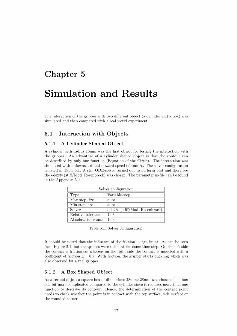
A cylinder with radius 15mm was the first object for testing the interaction withthe gripper. An advantage of a cylinder shaped object is that the contour canbe described by only one function (Equation of the Circle). The interaction wassimulated with a downward and upward speed of 4mm/s. The solver configurationis listed in Table 5.1. A stiff ODE-solver turned out to perform best and thereforethe ode23s (stiff/Mod. Rosenbrock) was chosen. The parameter m-file can be foundin the Appendix A.1.

Solver configuration

Type Variable-stepMax step size autoMin step size autoSolver ode23s (stiff/Mod. Rosenbrock)Relative tolerance 1e-3Absolute tolerance 1e-3

Table 5.1: Solver configuration.

It should be noted that the influence of the friction is significant. As can be seenfrom Figure 5.1, both snapshots were taken at the same time step. On the left sidethe contact is frictionless whereas on the right side the contact is modeled with acoefficient of friction µ = 0.7. With friction, the gripper starts buckling which wasalso observed for a real gripper.

5.1.2 A Box Shaped Object

As a second object a square box of dimensions 28mm×28mm was chosen. The boxis a bit more complicated compared to the cylinder since it requires more than onefunction to describe its contour. Hence, the determination of the contact pointneeds to check whether the point is in contact with the top surface, side surface orthe rounded corner.

17

Chapter 5. Simulation and Results 18

Figure 5.1: Comparison between a frictionless contact and a contact with µ = 0.7.The snapshots were taken at the same time step.

Figure 5.2 shows a snapshot series of the interaction with the box. The coefficientof friction in this series is µ = 0.6. After touchdown (≈ 1s) the gripper envelopesthe box and starts buckling. As soon as the tip is in contact with the side surface(≈ 3s) this buckling behavior stops and the right and left beam bend outwards.

Figure 5.2: Snapshot series of the interaction with the box. The coefficient offriction is µ = 0.6.

5.2 Validation of Linear Stress-Strain Relation

The lumped-parameter method proposed in Section 2.1 assumes a linear relationbetween stress and strain, described by the Young’s modulus E. Hence, this ap-proach is only applicable as long as stress and strain are in this linear region. Thissection shows that the following simulation results are valid because the estimatedstress-strain from bending measurements falls into the linear region of HMA. Notethat once leaving this linear region, the model could be extended if the stress-strainrelation is known. This relation can be experimentally determined as presented byBrodbeck et al. [1] where strain and stress of an HMA string were measured whenvariations of forces were exerted, shown in Figure 5.3. The stress-strain relationis linear if the strain is smaller than 0.2 or accordingly the stress is smaller than1.2 · 106Pa.In SimMechanics, the bending moments were measured with a joint sensor for boththe cylinder and the box. The largest measured bending moments are listed inTable 5.2.Using the relation between bending moment M and stress σ:

σ =M

I· z (5.1)

where z is the coordinate along the cross section, the maximum stress can be calcu-lated and will be at the top surface (zmax). These values are also listed in Table 5.2.It is obtained that the resulting stress is significantly smaller than the maximumstress of 1.2 · 106Pa for the linear region. Thus, the linear stress-strain relationshipis valid.

19 5.3. Results

Largest bending moment [Nm] Resulting stress [Pa]Box 5.41 · 10−3 2.9 · 105 < 1.2 · 106

Cylinder 3.82 · 10−3 2.0 · 105 < 1.2 · 106

Table 5.2: Largest bending moment and resulting stress for box and cylinder.

0 0.5 1 1.50

0.5

1

1.5

2x 10

6

Strain ε [−]

Nom

inal

Str

ess

σ n [Pa]

Figure 5.3: Tension test of an HMA string from Brodbeck et al. [1]. Linear relationuntil approximately σn = 1.2 · 106Pa.

5.3 Results

5.3.1 Linear Actuator Force

An interesting aspect of designing a passive compliant gripper may be the requiredlinear actuator force in order to pick up an object. The gripper geometry couldthen be optimized in a second step to reduce the maximum force that has to beapplied. Figure 5.4 shows measurements of the reaction force of the prismaticjoint for the cylinder and the box when the gripper moves towards the object withvelocity 4mm/s and a traveling distance of 28mm. Initially, the actuator force Fact

is negative since the weight of the gripper has to be supported. Afterwards, itincreases in both cases and reaches a maximum at a certain point. At time 7s thegripper has reached the lowest position.

Time [s]

Fact[N

]

Linear Actuator Force for Cylinder

0 1 2 3 4 5 6 7−0.1

0

0.1

0.2

0.3

0.4

0.5

0.6

(a) Cylinder.

Time [s]

Fact[N

]

Linear Actuator Force for Box

0 1 2 3 4 5 6 7−0.2

0

0.2

0.4

0.6

0.8

(b) Box.

Figure 5.4: Linear actuator force for cylinder/box (µ = 0.6).

Chapter 5. Simulation and Results 20

5.3.2 Angle of Deflection

To validate the model, the gripper was mounted on a robot arm and moved towardsthe exact same sized objects as discussed above. The angle of deflection ϕ(t) isdefined as the angle between the top beam and the right and left beam, respectively.In the simulation these two angles coincide since the geometry is symmetric. Theinitial angle of deflection ϕ0 = ϕ(t = 0) is shown on left in Figure 5.6. The simulatedangle over time is shown in the graphs of Figure 5.5. Again, the gripper reaches thelowest point at 7s and moves with velocity 4mm/s. This values for ϕ(t = 7s) arelisted in Table 5.3 in the column ‘Simulated angle’. The same angle was visuallymeasured from the experiment, shown on the right in Figure 5.6. The angle isdetermined on both left and right side because the experiment is not perfectlysymmetric. These values and its averages are also listed in Table 5.3 and comparedwith the simulated values which gives a relative error for the box of 1.9% and forthe cylinder of 1.5%.

Time [s]

ϕ(t)[◦]

Angle of Deflection for Cylinder

0 1 2 3 4 5 6 796

98

100

102

104

106

108

(a) Cylinder.

Time [s]

ϕ(t)[◦]

Angle of Deflection for Box

0 1 2 3 4 5 6 796

98

100

102

104

106

108

(b) Box.

Figure 5.5: Angle of deflection ϕ(t) for cylinder/box (µ = 0.6).

Real gripper experimentLeft angle Right angle Average Simulated angle Relative error [%]

Box 112.1◦ 106.9◦ 109.5◦ 107.4◦ 1.9Cylinder 110.3◦ 106.8◦ 108.6◦ 107.0◦ 1.5

Table 5.3: Angle of deflection during picking up for real world experiment andsimulation.

21 5.3. Results

Figure 5.6: Left: definition of the angle of deflection ϕ0 at time 0s. Right: angle ofdeflection ϕ(t = 7s) visually measured for the box and the cylinder at the lowestpoint.

Chapter 5. Simulation and Results 22

Chapter 6

Future Work

6.1 Force Closure Analysis

The current model does not consider whether or not the force closure of the gripper issufficient to pick up the object. This constraint could be implemented by knowingthe normal force FN and the frictional force FF before lifting the object. Theseforces can be measured in SimMechanics.The contact forces acting on the cylinder and the box are depicted in Figure 6.1.The lowest point of the gripper has no influence on the force composition in thecase of the box whereas for the cylinder the lowest point determines the directionof the contact forces. The contact point of the cylinder is described by an angle α.Adding up the force vectors results in a lifting force Flift,cyl in y-direction of:

Flift,cyl = 2FN sinα+ 2µFN cosα (6.1)

For the box, only the frictional force has a component in y-direction and thereforethe lifting force Flift,box is given by:

Flift,box = 2µFN (6.2)

The gripper is able to pick up the object if the lifting force is greater than theweight force of the object, i.e. Flift,box > mbox ·g and Flift,cyl > mcyl ·g , where mbox

is the mass of the box, mcyl is the mass of the cylinder and g is the gravitationalacceleration, respectively.

FN

FF

FN

FF

x

y FF

FN

FF

FN

x

y

Figure 6.1: Contact forces acting on the cylinder and box.

6.2 Design Optimization

Having a gripper model, this model can be used to run an optimization algorithm toget a new designed gripper which may have better properties regarding the process

23

Chapter 6. Future Work 24

of picking and placing a certain object. To do so, the model has to be generalizedto arbitrary parameters, e.g. the length of the beams, the angle between the beamsetc.

6.3 Auto-Detection of Object Contour

Further developments of the robot itself could also be a continuation of this project.This includes, for example, an auto-detection device for perceiving the object con-tour. By mounting a camera on the robot, following task could be accomplished:the robot has to pick and place a certain object. First, the camera detects the objectcontour and above mentioned optimization algorithm produces an optimal gripperfor that specific object. Afterwards, the fully automated glue supply mechanismmanufactures this optimal gripper and finally the robot is able to fulfill its task.

6.4 3D Modeling

The model may be extended to 3D. In that case, the lumped-parameter methodmay not be suitable anymore and other methods like FEM should be considered.For the grippers that are currently used at the BIRL, 2D modeling is sufficientsince the movement of the gripper is expected in only one plane. For other types ofgrippers this may not be the case anymore.

Appendix A

MATLAB Code

A.1 Parameters.m

The Parameters.m file has to be executed before running the model file.

1 %%%%%%%%%%%%%%%%%%%%%%%%%%%%%%%%%%%%%%%%%%%%%%%%%%%%%%%%%%%%%%%%%%%%%%%%%%%2 % Gripper Parameter File %3 %%%%%%%%%%%%%%%%%%%%%%%%%%%%%%%%%%%%%%%%%%%%%%%%%%%%%%%%%%%%%%%%%%%%%%%%%%%4

5 %%6 clear all7 close all8 clc9

10 rho = 0.98; % [g/cmˆ3]11 height = 0.7; % [cm]12 E = 8.9e6; % [N/mˆ2] Young's modulus HMA13 b = 0.01; % damping coefficient14 angle beam = 7; % [degree]15

16 %% Top17

18 l 1 = 0.21; % [cm]19 w 1 = 0.4; % [cm]20 m 1 = l 1*w 1*height*rho; % [g]21 I z1 = 1/12*0.01*height*(0.01*w 1)ˆ3; %[mˆ4]22 k 1 = E*I z1/(0.01*l 1); %spring [N*m/rad]23 J 1 = diag([0, 0, 1/12*m 1*(l 1ˆ2 + w 1ˆ2)]);24

25 % Drawing26 l 1 = 2.1; % [mm]27 w 1 = 4; % [mm]28

29 CS1 r = [0, 0, 0];30 CG r = [l 1/2, 0, 0];31 CS2 r = [l 1, 0, 0];32

33 CS2 r adjoin = [l 1 − w 1/2, −w 1/2, 0];34 CS2 l adjoin = [−l 1 + w 1/2, −w 1/2, 0];35

36 CS1 l = [0, 0, 0];37 CG l = [−l 1/2, 0, 0];38 CS2 l = [−l 1, 0, 0];39

40 %% Left Beam = Right Beam41

42 l 2 = 0.172; % [cm]43 w 2 = 0.4; % [cm]

25

Appendix A. MATLAB Code 26

44 m 2 = l 2*w 2*height*rho; % [g]45 I z2 = 1/12*0.01*height*(0.01*w 2)ˆ3; %[mˆ4]46 k 2 = E*I z2/(0.01*l 2); %spring [N*m/rad]47 J 2 = diag([0, 0, 1/12*m 2*(l 2ˆ2 + w 2ˆ2)]);48

49 %% Tip50

51 A t = 112*0.01; % [cmˆ2]52 m t = A t*height*rho; % [g]53 I t = 1/12*0.01*height*(0.01*w 2)ˆ3; %[mˆ4]54 k t = E*I t/(0.01*l 2); %spring [N*m/rad]55

56 J zz = 0.020395151; % [kg/mmˆ2] CAD57 J zz = 0.001/0.1ˆ2*J zz; % [g/cmˆ2]58 J t = diag([0, 0, J zz]);59

60 % CG61 CG t = [8.808687272, −2.331376882, 0]; % from CAD62

63 % Boundaries64 % Define coordinate systems on tip65 CS t1 = [5.150757595, −10.020815280, 0];66 CS t1 o = [0, 0, −135];67

68 CS t2 = [12.289596972, −5.710403028, 0];69 CS t2 o = [0, 0, −45];70

71 CS t3 = [7.979184720 ,−10.020815280, 0];72 CS t3 o = [0, 0, −45];73

74 CS t4 = [6.564971157, −10.606601718, 0];75 CS t4 o = [0, 0, −90];76

77 CS t5 = [14.443333542, −3.556666458, 0];78 CS t5 o = [0, 0, −45];79

80 CS t6 = [13.364995700, −4.635004300, 0];81 CS t6 o = [0, 0, −45];82

83 CS t7 = [11.214198244, −6.785801756 , 0];84 CS t7 o = [0, 0, −45];85

86 CS t8 = [10.135860402, −7.864139598 , 0];87 CS t8 o = [0, 0, −45];88

89 CS t9 = [9.057522561, −8.942477439, 0];90 CS t9 o = [0, 0, −45];91

92 CS t10 = [7.330338022, −10.454360783, 0];93 CS t10 o = [0, 0, −45 − 22.5];94

95 CS t11 = [5.799604293, −10.454360783, 0];96 CS t11 o = [0, 0, −135 + 22.5];97

98 CS t12 = [16.600009224, −1.399990776, 0];99 CS t12 o = [0, 0, −45];

100

101 CS t13 = [17.031748681, 0.770510047, 0];102 CS t13 o = [0, 0, −45 + 67.5];103

104 CS t14 = [17.138007330, −0.414256067, 0];105 CS t14 o = [0, 0, −45 + 32.75];106

107 %%108 % Dimension in mm for drawing109 l 2 = 1.72; % [mm]110 w 2 = 4; % [mm]

27 A.1. Parameters.m

111

112 CS1 b = [0, 0, 0];113 CG b = [l 2/2, 0, 0];114 CS2 b = [l 2, 0, 0];115

116 height = 7; % [mm]117

118 k Ground = 10000; % [N/m]119 b Ground = 1; % [Ns/m]120 mu Ground = 0.6;121 c = 10e−10; % [m/s]

Appendix A. MATLAB Code 28

Appendix B

CAD Drawing

B.1 Tip of the Gripper

The CAD drawing of the gripper’s tip is shown in Figure B.1:

Figure B.1: CAD drawing of the tip. All dimension in mm.

29

Appendix B. CAD Drawing 30

Bibliography

[1] L. Brodbeck, L. Wang, and F. Iida: Robotic body extension based on HotMelt Adhesives. Robotics and Automation (ICRA), 2012 IEEE InternationalConference on, pp. 4322-4327, May 2012.

[2] V. Chudnovsky, A. Mukherjee, J. Wendlandt, and D. Kennedy:Modeling Flexible Bodies in SimMechanics and Simulink. MatLab Digest, May2006.

[3] Sakai, S., Y. Nakamura, and K. Nonami: A pick-and-place hand mecha-nism without any actuators and sensors. 2007 IEEE International Conferenceon. IEEE, 2007.

[4] Sayir, Mahir, Jurg Dual, and Stephan Kaufmann: Ingenieurmechanik2: Deformierbare Korper. Vol. 2. Vieweg+ Teubner Verlag, 2009.

[5] Xiong, Cai-Hua, et al.: Compliant grasping with passive forces. Journal ofRobotic Systems 22(5), pp. 271-285, 2005.

[6] Petkovic, Dalibor and Pavlovic, Nenad D: Object grasping and liftingby passive compliant gripper. Mechanismentechnik in Ilmenau, Budapest undNis, pp. 55ff, 2012.

[7] Bicchi, Antonio, and Vijay Kumar: Robotic grasping and contact: Areview. Robotics and Automation, 2000. Proceedings. ICRA’00. IEEE Interna-tional Conference on. Vol. 1. IEEE, 2000.

[8] Chua, P. Y., T. Ilschner, and D. G. Caldwell: Robotic manipulationof food products – a review. Industrial Robot: An International Journal 30(4),pp. 345-354, 2003.

[9] Jacobsen, S. C., Wood, J. E., Knutti, D. F., and Biggers, K. B:The Utah/MIT dextrous hand: Work in progress. The International Journal ofRobotics Research 3(4), pp. 21-50, 1984.

[10] Heriban, David and Gauthier, Michael: Robotic micro-assembly of mi-croparts using a piezogripper. Intelligent Robots and Systems, 2008. IROS 2008.IEEE/RSJ International Conference on. IEEE, pp. 4042-4047, 2008.

[11] Bauchau, O. A., and J. I. Craig: Euler-Bernoulli beam theory. StructuralAnalysis. Springer Netherlands, pp. 173-221, 2009.

[12] Szabo, Barna and Babuska, Ivo: Introduction to finite element analysis.John Wiley and Sons, New York, 1991.

[13] Datasheet: Henkel.: Technisches Merkblatt - Pattex Hot Sticks Transparent.2008.

31

Bibliography 32

[14] Vielsack, P.: Regularisierung des Haftzustandes bei Coulombscher Reibung.ZAMM-Journal of Applied Mathematics and Mechanics/Zeitschrift fur Ange-wandte Mathematik und Mechanik 76(8), pp. 439-446, 1996.