2D arrays and Volume Focusing Combined Inspection Technique.

Dominique Braconnier, Masaki Takahashi, KJTD co. Ltd,

9-29 Sumida 1 chome, Higashiosaka , osaka, Japan , 578-0912 dbraconnier@indes-ndt.com

Abstract:

2D arrays, also called matrix arrays, have recently appeared on the market providing key advantages to improve inspection methods and results. In particular, point focus ability, tilt and skew angle scanning are both promising features that new electronic equipment makers are promoting. Volume Focusing, when used with 2D arrays, yields high inspection speeds, interaction of UT waves and flaws, and the ability to image an entire volume of material without moving the probe. This paper presents such a situation, with results based on using a few 2D Phased arrays, as well as different test pieces to prove the feasibility. Detection as well as resolution abilities, in addition to speed issues are discussed to present not only qualitative, but quantitative data.

Key words:

Phased Array; Matrix; 2D; Ultrasonic; Inspection; Weld; Volume Focusing; Skew deflexion; point focus;

Introduction:

This paper will present results obtained with 2D arrays. At first, a quantitative comparison between linear and matrix probes from testing done at JAPEIC is reported.

Secondly, qualitative data are shown in comparison between the point focus technique, DDF (Dynamic Depth Focusing) and Volume Focusing to show the interest and limitation of each one.

In the Third part, Volume Focusing is applied on slit detection and sizing inside a weld, showing advantages in comparison with techniques commonly used nowadays.

The main objective is more to show some of the possibilities offered by Volume Focusing, than to describe a specific application.

17th World Conference on Nondestructive Testing, 25-28 Oct 2008, Shanghai, China

Comparison of sizing ability between Linear probe and Matrix from experiment with real flaw in JAPEIC:

10 sample tests were inspected by an inexperienced operator by conducting a blind test with linear probes during a training session in JAPEIC. The inspection took in the range of 2 and half hours. The same test pieces were inspected once more, another day, with Matrix phased Array, spending almost the same inspection time as the linear probe inspection, in the range of 2 and half hours. Table 1 shows the difference between the measured flaw height and the real flaw height for each technique used, Linear and Matrix.

Sample A B C D E F G H I J

Linear -0.18 -0.58 -0.93 0.09 1.56 -0.9 0.9 2.77 1.25 -1.9

Matrix 1.96 -0.18 1.78 -1.78 3.48 -1.08 0.24 -1.42 3.29 0.68

Combined -0.18 -0.18 -0.93 0.09 1.56 -0.9 0.24 -1.42 1.25 0.68

Table 1: Comparison of flaw height measurement error (in mm) between linear and matrix probes without correlation between the 2 techniques during the test.

We can conclude that in both cases, the size errors are quite small, and the inspection time is very small according to the complexity of the task. We can also notice that the 2 inspection sessions (linear and matrix) were done at 2 different times with different orders and without keeping the knowledge of the results, resulting in an uncorrelated outcome. Correlation would have probably helped a lot to reduce the variance in the flaw height.

Description of the method and tools used for the experiment:

Phased Array technology is based on sampling the surface of the probe in small elements that act as punctual probes transmitting to and receiving from any direction, and whose signals can be phased in a way that the UT beam has the characteristics the operator wishes. Symmetrical electronic lenses allow focusing at the desired depth, taking in account the wedge and part refracting interface. Dissymmetrical lenses allow deflecting the beam along a different axis of propagation from the natural axis of the probe.

Phased array does have limitations. If elements are too large versus the wavelength, the ability to focus or deflect will be limited, because the element will have sensitivity only in front of the transducer. However, the focusing and deflection ability of phased array is usually very profitable to provide images without moving the probe, with very good accuracy and clarity. Besides, scanning with phased array can capture overlaps between images with different positions, so that the immunity of the analysis to the speckle noise improves by a significant factor.

2D arrays (see figure 1&2), also called “matrix phased arrays” are constituted of 2-dimentional sampling of the surface of the probe. They are still very rare, because the 2 dimensional sampling leads to a number of elements proportional to the square of what would be necessary for a linear (1D) phased array to sample the surface of the probe, and it is still hard to find electronic instruments that can drive enough elements to produce meaningful results with matrix probes. However, when a matrix is well designed, it allows having a point focused beam, defined with 3-D parameters, and deflection along the axis with any tilt and skew angle along the depth in front of the probe at the same time.

Figure 1: 2D phased array with Rho Theta definition example

Figure 2: 2D phased array with TRL Rho Theta definition example

A word on Volume Focusing:

Volume Focusing consists of firing all element of the probe, collecting each individual signal from the element of the probe, and making mathematical processing on all signals combined together. With a matrix (2D array), as only one transmitted pulse irradiates through the volume, it is possible by calculation to form the beams that inspect this volume. This calculation is done in real time inside the electronics, and only the results are sent to the computer so that the visualization is sped up.

The beam calculation usually consists of calculating several sector scans with different definitions of incidence, range and focus depth. DDF (Dynamic Depth Focusing) is compatible with Volume Focusing.

One of the advantages of this technique is the gain in inspection speed. Indeed, to provide lots of beams, possibly from different sequences, only 1 transmitted pulse is required, and the calculation of the beam is done inside the electronic instrument so that it can be done with ultra-fast processing. This is illustrated with figure 3.

Figure 3: Comparison of conventional Phased array acquisition in the left, and with Volume Focusing in the right with a sequence of 97 cycles.

For the experiment, the following items were used:

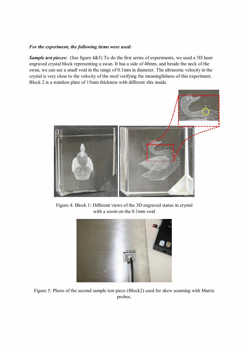
Sample test pieces: (See figure 4&5) To do the first series of experiments, we used a 3D laser engraved crystal block representing a swan. It has a side of 40mm, and beside the neck of the swan, we can see a small void in the range of 0.1mm in diameter. The ultrasonic velocity in the crystal is very close to the velocity of the steel verifying the meaningfulness of this experiment. Block 2 is a stainless plate of 15mm thickness with different slits inside.

Figure 4: Block 1: Different views of the 3D engraved statue in crystal with a zoom on the 0.1mm void

Figure 5: Photo of the second sample test piece (Block2) used for skew scanning with Matrix probes.

Probes. 2 kinds of matrix probes were used: a linear square sampling 2MHz matrix (IMASONIC 64 elements) and 2 Matrix RhoTheta (IMASONIC 5MHz 128 elements each, Active aperture of respectively 15mm and 20mm).

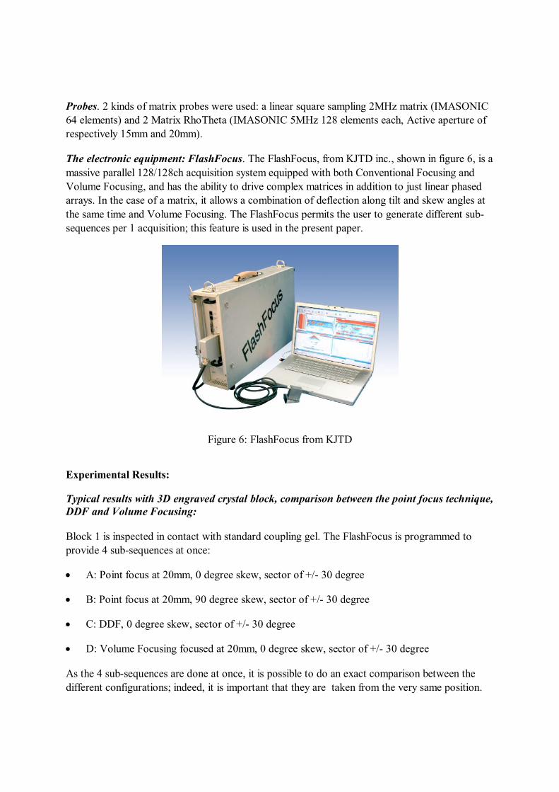
The electronic equipment: FlashFocus. The FlashFocus, from KJTD inc., shown in figure 6, is a massive parallel 128/128ch acquisition system equipped with both Conventional Focusing and Volume Focusing, and has the ability to drive complex matrices in addition to just linear phased arrays. In the case of a matrix, it allows a combination of deflection along tilt and skew angles at the same time and Volume Focusing. The FlashFocus permits the user to generate different sub-sequences per 1 acquisition; this feature is used in the present paper.

Figure 6: FlashFocus from KJTD

Experimental Results:

Typical results with 3D engraved crystal block, comparison between the point focus technique, DDF and Volume Focusing:

Block 1 is inspected in contact with standard coupling gel. The FlashFocus is programmed to provide 4 sub-sequences at once:

· A: Point focus at 20mm, 0 degree skew, sector of +/- 30 degree

· B: Point focus at 20mm, 90 degree skew, sector of +/- 30 degree

· C: DDF, 0 degree skew, sector of +/- 30 degree

· D: Volume Focusing focused at 20mm, 0 degree skew, sector of +/- 30 degree

As the 4 sub-sequences are done at once, it is possible to do an exact comparison between the different configurations; indeed, it is important that they are taken from the very same position.

A, C and D: B:

A, C and D: B:

Figure 7: Wizard views of each A, B, C and D configuration of scanning

In this section, all results of the Sscans are represented in the same way as shown in figure 8.

Figure 8: Layout showing sector scan of each A, B, C and D configuration of scanning

(A) Point focus at

20mm, 0 degree skew, sector of +/-

30 degree

(C)

DDF, 0 degree skew, sector of +/-

30 degree

(B) Point focus at

20mm, 90 degree skew, sector of +/-

30 degree

(D) Volume Focusing

focused at 20mm, 0 degree skew, sector

of +/- 30 degree

A series of views taken from different positions permits one to make a qualitative comparison between the different configurations (techniques).

Figure 9: The Matrix probe is positioned above the head of the swan along 90 degrees from the axis of the plane defined by his neck.

From figure 9, we can see clearly in configuration (B) the upper (1) and lower (2) cut view of the neck of the swan, as well as the cut (3) of the body of the swan clearly showing its tail (4). In configurations (A), (C) and (D), as the skew is the same, it must represent the same thing. In configuration (A), we can notice also the upper (1) and lower (2) cut view of the neck of the swan, and the top of the wings (5), as well as a cut of the body (6) of the swan that is more or less represented by a circle.

As the block has a 40mm side, 20mm corresponds to a focusing in the middle of the block.

In the case of DDF (configuration C), we can notice a lower sensitivity than the configuration focused at 20mm (A), but a longer depth of field. As the theory predicts, it also seems that the lateral resolution of the DDF case is better before and after the focused zone of the configuration (A), that is to say 20mm.

In the case of Volume focusing (configuration D), we can notice again a decrease in sensitivity and the lateral resolution becomes larger, but the depth of field is excellent.

1 2

3 4

5

6

Figure 10: The Matrix probe is positioned above the head of the swan along the axis of the plane defined by his neck (90 degree orientation from figure 9).

Figure 10 shows results with inversions between configurations (A) and (B) as the probe was turned by 90 degrees: we can see clearly in all the upper (1) and lower (2) cut view of the neck of the swan. In the configurations (A), (C) and (D) the cut (3) of the body of the swan and clearly its tail (4) is displayed. The configuration (A), (C) and (D), as the skew is the same, must represent the same thing. In the configuration (B), we can notice also the upper (1) and lower (2) cut view of the neck of the swan, and the top of the wings (5), as well as a cut of the body (6) of the swan that is more or less represented by a circle.

The statement remains the same from the previous figure analysis. DDF (configuration C) presents a better lateral resolution along the whole depth of field. Volume Focusing presents an excellent depth of field, but with degradation of the sensitivity and of the lateral resolutions.

1 2

3 4

5

6

a b

Figure 11: The Matrix probe is moved with different angles from the previous figures

to take different point of views.

In figure 11, the acquisition was done in the same way as the previous figures, but by turning the probe + or – 45 degrees for figure 11a, and changing the location for figure 11b. Basically, the assessment is the same as the previous views.

a

b

Figure 12: The Matrix probe is moved at different locations, above the 0.1mm void beside the neck of the swan.

Figure 12 differs from the previous ones where the matrix is now located above the 0.1mm void that is located beside the neck of the swan. We can confirm this fact because configuration (A) and (B) with a 90 degree skew difference shows the same echo from void (1).

In figure 12a (left), we can see the void with a relatively good S/N for configuration (A) and (B), but is unclear for configuration (C) and (D). This is to say that the DDF has good depth of field

1

2

and relatively good lateral resolution, but not good enough to properly detect the void located at a depth of 12mm. The same assessment is done for the case of Volume Focusing.

In figure 12b (right), a change was done in configuration (D) for Volume Focusing. In this case, the focus was changed to DDF and at the same time, the aperture was limited to 64 elements instead of 128 elements. Due to this change, it is now possible to clearly detect void (2) with a relatively good S/N.

Typical results using Volume focusing to make Skew scanning looking for slit in block2:

Here is an overview of typical results for different obliquities of the slits.

A B

C D

Figure 13: Wizard view of the 2 configurations, conventional Sector scan A, B and Skew mode scan in Volume Focusing mode C (perspective), D (Top view).

The probe is now moved on the plate (Block2) in contact through a wedge with a wire encoder to record the position. This time, the sequence contains 2 sub-sequences. The first subsequence is a usual sector scan with a tilt angle varying from 30 to 60 degrees. The second sub-sequence is done in Volume Focusing mode with a skew mode scanning, that is to say that the beam is scanned with the skew angle moving, and tilt angle fixed, at the contrary from the previous experiments where all sector scans were obtained with a fixed skew.

Figure 14: View of the sector scan sub-sequence on 5mm slit.

The slit tip echo (1) and corner (2) echo appear clearly in the Sector scan as well as in the Bscan. So, placing the cursor on the right depth range, the Cscan which is actually only 1 line (because the mechanical scan is parallel to the sector scan), also shows the slit tip and corner echo very clearly.

Figure 15: View of the Skew mode scan Volume Focusing sub-sequence from the same scan than the figure 13.

In the case of the sub-sequence from the Volume Focusing skew mode scan, we can see from figure 14 that the slit on the Sector scan and on the Cscan is not only 1 point but a line. The Bscan shows also the tip (1) of the slit as well as the corner (2) echo.

At last, figure 15 shows exactly the same result, but on 1 layout, all acquisitions are done in the same sequence.

Sector scan

Bscan

Cscan

Skew mode VF Sector scan

Bscan

Cscan

1

2

1

2

1

2

1 2

Figure 16: View of the combination of Skew mode scan Volume focusing sub-sequence and conventional sector parallel scan sub-sequence.

We then compare the result with different orientations of the slit:

Figure 16: View of the combination of Skew mode scan Volume focusing sub-sequence and conventional sector parallel scan sub-sequence with the slit at 0 degree skew.

From figure 16 to 18, the slit orientation is 0, 10 and 20 degrees. We can see from the Volume Focusing results on the Cscan that the slit is indeed shifted to one side. The main effect on the conventional sector scan is that the angle where the signal becomes the highest is lower when the slit is more angled. In addition, the sensitivity decreases.

Looking at just print-screens do not allow us to completely see the merit of the technique, but from the point of view of an operator, it is very easy to detect and size the flaw with the Volume Focusing view, and receive confirmation with the conventional sector scan.

VF Bscan

VF Cscan VF Sscan

Figure 17: View of the combination of Skew mode scan Volume focusing sub-sequence and conventional sector parallel scan sub-sequence with the slit at 10 degree skew.

Figure 18: View of the combination of Skew mode scan Volume focusing sub-sequence and conventional sector parallel scan sub-sequence with the slit at 20 degree skew.

Conclusion

According to our experience, with a conventional point focus technique, Matrix phased Array with a large amount of small elements provide more or less the same sizing ability as the best linear Phased Array, that we can conceive. However, for real flaws with a very small height such as SCC of less than 3mm, the Matrix provides more comfort to the operator.

A qualitative comparison with the Point Focus technique, DDF and Volume Focusing shows an overall decrease in sensitivity. The lateral resolution of DDF remains the best for the overall depth of field, but Volume Focusing offers the best depth of field.

VF Bscan

VF Cscan VF Sscan

VF Bscan

VF Cscan VF Sscan

Concerning the inspection speed, there is nothing to compare with the speed of the Volume Focusing technique.

Lastly, Volume Focusing when used for disoriented flaws clearly shows its advantages. The orientation of the flaw is directly accessible from the image, which creates more comfort in detecting and sizing.

It is planned to continue the present comparison experiments with natural flaws such as SCC and boundary surface area echoes and cracks. This technique opens a new field of inspection that can speed up the inspection not only by reducing the scanning acquisition time, but also more importantly by reducing the analysis time, providing in addition more self-confidence to the operator.

References

1. Takeko Murakami, Dominique Braconnier, KJTD ltd. The new technology of high speed ultrasonic detection flaw by array, 2005. 13-13, Nishiikebukuro 5-Chome, Toshima-ku, Tokyo, Japan, 2005.

2. Junichiro Nishida, MITSUBISHI HEAVY INDUSTRIES LTD., Yoichi Iwahashi, Takanori Yamashita, E-TECHNO, Dominique Braconnier, KJTD, Inspection of thick part with Phased Array Volume Focusing technique, EPRI USA May 2006.

1. Eiichi Yonetsuji, Takeko Murakami, Dominique Braconnier, KJTD ltd. Inspection of thick part with Phased Array Volume Focusing technique, 2005. 13-13, Nishiikebukuro 5-Chome, Toshima-ku, Tokyo, Japan, November 2006.

Acknowledgments

We would like to thank in particular JAPEIC: Yamaguchi san, Yoneyama san and Sugibayashi san for their kind support.