29 Aberrations - Wiley-VCH · 29 Aberrations In spite of the fact that wavefront aberrations are...

1

29.1 Introduction 2

29.2 Power Series Expansions 8

29.3 Chromatic Aberrations 13

29.4 Primary Aberrations 16

29.4.1 Aperture and Field Dependence 16

29.4.2 Symmetry and Periodicity Properties 18

29.4.3 Presentation of Aberrations and their Impact on Image Quality 20

29.4.4 Calculation of the Seidel Sums 29

29.4.5 Stop Shift Formulae 36

29.4.6 Several Aberration Expressions from the Seidel Sums 38

29.4.7 Thin Lens Aberrations 41

29.5 Pupil Aberrations 45

29.6 High-order Aberrations 50

29.6.1 Fifth-order Aberrations 50

29.6.2 Seventh and Higher-order Aberrations 53

29.7 Zernike Polynomials 55

29.8 Special Aberration Formulae 56

29.8.1 Sine Condition and the Offence against the Sine Condition 57

29.8.2 Herschel Condition 60

29.8.3 Aplanatism and Isoplanatism 61

29.8.4 Aldis Theorem 61

29.8.5 Spherical Aberration, a Surface Contribution Formula 64

29.8.6 Aplanatic Surface and Aplanatic Lens 68

29.9 Literature 70

29

Aberrations

Handbook of Optical Systems: Vol. 3. Aberration Theory and Correction of Optical Systems.Edited by Herbert GrossCopyright © 2007 WILEY-VCH Verlag GmbH & Co. KGaA, WeinheimISBN: 978-3-527-40379-0

29 Aberrations2

29.1Introduction

In this and in the following section (29.2) we will deal with monochromatic aberra-tions only. In section 29.3 chromatic aberrations will be introduced and will then beincluded in our further discussions. As we have already explained in chapter 11, ingeneral, a real optical imaging system does not perform ideal imaging. So, raysemerging from one object point O will not all meet at a single image point O′. Anexample with three meridional rays is shown in figure 29-1.

O'

O

optical

system

Figure 29-1: Aberrations of an imaging system.

There are several methods used to describe how the rays miss the image point, seesection 11.2, Description of Aberrations. Very often it is convenient to think in terms oftransverse aberrations. Consider a single object point and a given position of the imageplane and on this plane consider a given reference point, which is the point where theimage should be. Usually the assumed image point will be the Gaussian image point,but this is in fact not necessary. The position of the image plane as well as the choice ofthe image reference point may differ from the Gaussian values if required. For instance,one reason for choosing the Gaussian image plane but not the Gaussian image heightmay be some distortion if distortion is not of interest. In this case the intersection of thereal chief ray with the image plane may be adequate as the image reference point. A verycommon reason for choosing image planes, which are different from the Gaussianimage plane, is to study the behavior of the aberrations with a change in the focus.

There are several ways to present transverse aberrations in graphical form. Wewill outline some examples for a very simple system, a single biconvex lens asshown in figure 29-2. Two field points are considered, one field point is on the axis,while the second field point is off the axis.

Figure 29-2: Biconvex lens, f ′ = 100 mm, F/5, image height 5 mm.

29.1 Introduction

Spot diagrams are a very popular way of presenting transverse aberrations, seefigures 29-3 and 29-4. The through-focus spot diagrams show the characteristics ofa lot of aberrations and suggest the size of the image blur. However, even with thissimple example, it can be seen that the impression of the ray intersection spotsstrongly depends on the chosen ray distribution in the pupil. For figure 29-3 arectangular pupil grid is used and for figure 29-4 a polar pupil grid is used.

Image height

5 mm

0 mm

Defocus ( mm ) - 0 . 5 - 0.25 0 0.25 0.5

0.4 mm

Used pupil grid :

Rectangular

Figure 29-3: Through-focus spot diagram with rectangular pupil grid.

Image height

5 mm

0 mm

Defocus (mm) -0.5 -0.25 0 0.25 0.5

0.4 mm

Used pupil grid :

Polar

Figure 29-4: Through-focus spot diagram with polar pupil grid.

3

29 Aberrations

In general it is difficult to distinguish typical aberrations from spot diagrams.However, for this purpose the transverse aberration fans are an adequate means, seefigure 29-5. Here the transverse aberrations of two pupil sections are represented:For the on-axis image the ray bundle is symmetric with respect to the optical axis, soall information is contained in the presentation of the meridional section only. Themeridional pupil section is also called the tangential pupil section. For an imageheight of 5 mm, in the tangential pupil section, due to the rotational symmetry ofthe system, all aberrations are in the image y-direction. From the sagittal pupil sec-tion the rays have aberration components � y′ in image y-direction as well as compo-nents � x′ in the image x-direction and these components exhibit characteristic sym-metries (point symmetry and mirror symmetry, respectively) as shown in figure29-5. Usually, for the sagittal section, only the more important x-component of theaberration is shown. As will be explained later, the transverse aberration fans infigure 29-5 are clearly dominated by spherical aberration and also by coma.

Image

height 0 mm 5 mm 5 mm 5 mm

Aberration ∆ y' ∆ y' ∆ x' ∆ y'

Pupil section meridional meridional sagittal sagittal

0.2 mm 0.2 mm 0.2 mm 0.2 mm

Figure 29-5: Transverse ray aberrations.

The use of transverse aberrations is a powerful method and all types of aberration,such as spherical aberration, coma, astigmatism, field curvature and distortion, aswell as axial chromatic aberration and lateral chromatic aberration can be under-stood and represented as transverse aberrations.

Nevertheless, there are situations where it is desirable to use longitudinal aberra-tions. For instance, astigmatism and field curvature are easily understood as longitu-dinal phenomena. But spherical aberration, coma, and axial chromatic aberrationcan also be understood as longitudinal aberrations. Figure 29-6 shows the sphericalaberration and the astigmatic field curves of the system considered in figure 29-2 aslongitudinal aberrations. The only aberrations, which cannot be described as long-itudinal aberrations, are distortion and lateral chromatic aberration.

4

29.1 Introduction

2.0-2.0 0.0

Spherical aberration Tangential & sagittal field

z ∆ ∆

Aperture

-2.0 2.00.0

z

Field

T S

Figure 29-6: Longitudinal ray aberration curves.

For optical systems which image to infinity, the transverse as well as the longitu-dinal aberrations do not make sense, as they both become infinite. In this case, forthe image at infinity, instead of transverse aberrations measured in length units,angular aberrations measured in angle units will be adequate. So angle aberrations,which were introduced in section 11.2, Description of Aberrations, correspond totransverse aberrations and exhibit the respective properties. Also, for longitudinalaberrations there is an adequate representation when the image is at infinity:Instead of the longitudinal aberration itself, the reciprocal value of the intersectionlengths is used. As the unit of dimension diopters are normally used. To express anintersection length S′ in diopters, S′ should be measured in m. Then the corre-sponding value �S′ in diopters is defined as

�S′ diopter� � � 1S′ m� �. (29-1)

So aberrations measured in diopters correspond to the longitudinal aberrations. Forinstance, in vision optics, diopters are the preferred aberration description.

Transverse and longitudinal ray aberrations are easy to understand, and they rep-resent a complete and powerful method of describing the aberrational behavior ofan optical imaging system. So, for what reason do we need wave aberrations? Thereare, in fact, some specific advantages connected with the understanding and the useof wave aberrations. The most important benefits of a description based on waveaberrations are as follows.

� Wavefront aberrations can be measured very easily and very accurately bymeans of interferometric methods. This is a big advantage because the mea-surement of ray aberrations with any comparable completeness and accuracyis almost impossible.

5

29 Aberrations

� In spite of the fact that wavefront aberrations are strictly a geometrical opticsmethod there is a strong relationship to physical image formation. Aspointed out in chapter 12, the wave aberration is the essential input for calcu-lating the diffraction image. As an aberration-free system would image anobject point not as a single image point but as the Airy pattern, it is under-standable that very small aberrations would not change the Airy pattern sig-nificantly. In this case the image quality is determined more by diffractioneffects than by geometrical aberrations. When working with wave aberrationsthere is a very useful rule of thumb, the so-called Rayleigh limit: If the waveaberration is less than one quarter of the wave length, the system can beregarded as diffraction limited.

� When considering surface contributions, wave aberrations are convenient inthat the single surface contributions sum up directly to the total aberration. Itis possible to obtain a surface contribution formula for transverse aberra-tions, see section 29.8.4, Aldis Theorem, but these formulae are not as plausi-ble as are the wave aberrations.

� Finally, aberration theory informs us that there are distinct types of aberra-tions such as spherical aberration, coma, astigmatism, etc. For the proof ofthis statement, see section 29.2, where we show that wave aberrations aremuch more convenient than ray aberrations.

Consider an imaging system and a single object point O. Instead of investigatingthe rays itself emerging from the object point, we now look into the behavior of thewavefronts. In principle, there is no new information about the aberrations, as thewavefronts are strictly connected to the rays. The wavefront is defined as the locusof a constant optical path measured from the object point. As a reminder: the opticalpath is the geometrical distance multiplied by the local refractive index. It can beshown that the wavefronts are usually perpendicular to the rays. So in object space,where all rays pass through the object point, the wavefronts have the shape of con-centric spheres, with the object point as center. In image space, when there are noaberrations at all, the wavefronts are again spheres, centered on the image point. Inthe case of aberrations, the wavefronts in the image space are no longer spheres,and the deviation to a suitable reference sphere is the wave aberration. There issome arbitrariness in choosing the reference sphere, but in practice this is not aproblem. According to figure 29-7 the reference sphere is determined by its centerO′, which is the assumed image point, and by its radius R. Usually the radius R ischosen so that the reference sphere contains the intersection point of the chief raywith the optical axis, point Q in figure 29-7, that is the location of the exit pupil. Inthe case of an infinite image, as the image point is at infinity, the radius R becomesinfinite and the reference “sphere” becomes a plane, perpendicular to the chief ray.

6

29.1 Introduction

O

O'P

Q

B

R

Chief ray

Figure 29-7: Wave aberrations.

We denote the optical path length from the object point O to a point B by [OB].From figure 29-7 it can be seen that

[OB] = [OQ] (29-2)

as B and Q are points on the same wavefront. So, the wave aberration W is definedas the optical path along the ray from the reference sphere to the wavefront:

W = [OB] – [OP] = [OQ] – [OP]. (29-3)

An alternative designation for the wave aberration W is the optical path differenceOPD = W.

The given procedure used to determine the reference sphere radius R, using theposition of the exit pupil, breaks down when the imaging system is telecentric inthe image space. In this case the chief rays are parallel to the optical axis and theexit pupil is at infinity. Nevertheless for telecentric systems it also makes sense todefine wave aberrations relative to a reference sphere. Since for practical use theactual size of the reference sphere radius R is unimportant, the radius can be chosento have any plausible size. The only thing that must be avoided is a reference sphereradius that is too small, which means that the reference sphere should be farenough from the focal region where the rays from the imaging ray bundle intersecteach other. An example is shown in figure 29-8.

The graphical presentation of the wave aberration for the same example as shownin figure 29-2 is given in figure 29-9.

7

29 Aberrations

Chief ray O'

Optical

system

R

Optical axis

Image

plane

Figure 29-8: Wave aberration and reference sphere for a systemwhich is telecentric in the image space. The aberrations arestrongly exaggerated for clarity.

Image

height 0 mm 5 mm 5 mm

Pupil section meridional meridional sagittal

10 λ 10 λ 10 λ

Figure 29-9: Wave aberrations for the system in figure 29-2.

29.2Power Series Expansions

The wave aberration clearly depends on the chosen ray. When the wave aberrationfor all rays emerging from the object point O and passing through the exit pupil isto be described, the rays concerned are identified by their pupil coordinates xp andyp and the wave aberration W(xp,yp) is a function of two variables. It must be pointedout that this function W(xp,yp) only describes the aberrational behavior for the fixedchosen object point. To obtain complete information about the system aberrations

8

29.2 Power Series Expansions

one has to consider not only one object point but the whole object field. If we char-acterize an object point by its object plane coordinates x and y, then the wave aberra-tion becomes a function of four variables W(x,y,xp,yp). This function of four vari-ables is really necessary when optical systems without rotational symmetry are to beinvestigated [29-1]. In the more usual case, when the rotational symmetry of theoptical system is given, there is redundancy in the four variables. In figure 29-10 wewill see that, in this case, three variables are actually needed to describe the systemsaberrations completely.

Object

x

y

F

y

x

FϕPupil

P

xp

yp

z

yp

xp

Pϕ

Figure 29-10: Equivalent rays by rotational symmetry.

In figure 29-10, from the rotationally symmetric optical system, only the objectplane and the pupil plane are shown. We regard a single ray with object coordinatesx and y and pupil coordinates xp and yp (the red ray in figure 29-10). For this ray thewave aberration is denoted by W(x,y,xp,yp). Now, when this ray is rotated about theoptical axis by an arbitrary amount (the green ray in figure 29-10), due to the rota-tional symmetry of the system, the wave aberration will not change. So, instead ofdescribing the ray by the four variables x, y, xp, and yp, the Cartesian object and pupilcoordinates, we have to find adapted variables which are invariant with respect torotation about the optical axis. Let �F indicate the object vector from the object planeorigin to the object point (x, y) and �P the pupil vector from the pupil plane origin tothe pupil point (xp,yp). Let the lengths of these vectors be F and P respectively, thensuch rotationally invariant variables are:

9

29 Aberrations

� the square of the object or field vector length �F ��F � F2 � x2 � y2

� the square of the pupil vector length �P ��P � P2 � x2p � y2

p� the scalar product of the field vector and the pupil vector

�P ��F � P � F � cos ��F � �P� � xp � x � yp � y.

The last quantity �P ��F contains not only the lengths of the field and pupil vectors,but also the angle �F � �P between these two vectors.

With these new variables the wave aberration for an arbitrary ray can be writtenas W � W��P ��P��P ��F��F ��F�.

As the wave aberration is now dependent only on the length of the object vector,on the length of the pupil vector, and on the angle �F � �P between the object andpupil vector, without loss of generality we can choose the object point on the y-axis.So, we set x = 0 and for the wave aberration we obtain

W � W�x2p � y2

p� ypy� y2�. (29-4)

In eq. (29-4) y represents the object field coordinate. In the case of an object at infi-nity y should be understood as the object field angle. The function (29-4) can now beexpanded as a power series in three variables, arranging the terms in the properorder we get:

W � W�x2p � y2

p� ypy� y2�W � a0 � b1�x2

p � y2p� � b2yyp � b3y2

� c1�x2p � y2

p�2 � c2yyp�x2p � y2

p� � c3y2y2p � c4y2�x2

p � y2p� � c5y3yp � c6y4

� d1�x2p � y2

p�3 � d2yyp�x2p � y2

p�2 � d3y2y2p�x2

p � y2p� � d4y2�x2

p � y2p�2 � d5y3yp�x2

p � y2p�

� d6y3y3p � d7y4y2

p � d8y4�x2p � y2

p� � d9y5yp � d10y6

� terms with higher order�

(29-5)

The designation of the expansion coefficients ai, bi, ci, di,... corresponds to the sumof the powers in the variables. Going back to the original Cartesian coordinates y, xp,and yp, the total powers are zero for a0, two for bi, four for ci, and six for di. It will beshown that the bi terms represent the primary aberrations and the ci represent thesecondary aberrations.

This power expansion is strictly mathematical. As the wave aberration is not anarbitrary function to be expanded, but is defined in such a way that it vanishes at thepupil center (xp= yp = 0), all coefficients in expressions with no dependence on thepupil coordinates must be zero. So, a0, b3, c6, d10,... are set to zero.

This procedure of ignoring the terms which only depend on the field coordinate,when setting the coefficients b3, c6, d10,...to zero, may appear a little strange. Usuallymathematical results have some physical meaning. As we will see in section 29.5,these terms will actually have meaning when the pupil aberrations are addressed.

For some further discussion it is advantageous to express the pupil dependenceof the wave aberration not only in Cartesian coordinates as in (29-5) but also in polarcoordinates. As shown in figure 29-11 we define the length of the pupil vector r andthe azimuth angle � as

10

29.2 Power Series Expansions

yp

xp

rϕ

Figure 29-11: Polar coordinates for the pupil.

r ��x2

p � y2p

�(29-6)

xp � r � sin�

yp � r � cos��(29-7)

In terms of polar coordinates in the pupil the wave aberration W reads:

W � b1r2 � b2yr cos�

� c1r4 � c2yr3 cos�� c3y2r2 cos 2�� c4y2r2 � c5y3r cos�

� d1r6 � d2yr5 cos�� d3y2r4 cos 2�� d4y2r4 � d5y3r3 cos�

� d6y3r3 cos 3�� d7y4r2 cos 2�� d8y4r2 � d9y5r cos�

� terms with higher order�

(29-8)

According to eqs (11-12) and (11-13) the transverse ray aberrations � x′ and � y′ canbe calculated to a good approximation by differentiating the wave aberration withrespect to xp and yp , respectively:

� x ′ � � Rn′

� ∂W∂xp

, (29-9)

� y′ � � Rn′

� ∂W∂yp

, (29-10)

where R is the radius of the reference sphere and n′ is the refractive index in imagespace. The approximation inherent in eqs (29-9) and (29-10) is adequate for derivingthe primary transverse aberrations. In the case of vanishing primary aberrations,eqs (29-9) and (29-10) can also be used to derive the secondary transverse aberra-tions. So, applying these equations to (29-5) the power series expansion of the trans-verse ray aberrations can be derived:

11

29 Aberrations

� x ′ � � Rn′

2b1xp � 4c1xp�x2p � y2

p� � 2c2yxpyp � 2c4y2xp � ��

(29-11)

� y′ �� R

n′2b1yp � b2y � 4c1yp�x2

p � y2p� � c2y�x2

p � 3y2p� � 2�c3 � c4�y2yp � c5y3 � ��

� ��

(29-12)

With the help of eqs (29-6) and (29-7) and using the identities (29-13) and (29-14)

2 cos 2� � 1 � cos 2�, (29-13)

2 sin� cos� � sin 2�, (29-14)

the transverse aberrations � x ′ and � y′ can be expressed in polar coordinates in thepupil:

� x ′ � � Rn′

2b1r sin�� 4c1r3 sin�� c2yr2 sin 2�� 2c4y2r sin�� (29-15)

� y′ � � Rn′

2b1r cos�� b2y � 4c1r3 cos�� c2yr2�2 � cos 2�� 2�c3 � c4�y2r cos�� c5y3 � �� (29-16)

In the power series expansions eqs (29-5), (29-8), (29-11), (29-12), (29-15),(29-16) thesingle summands are clearly distinguished by the different powers of the field vari-able y and of the pupil variables xp and yp for Cartesian coordinates in the pupil andr for polar coordinates in the pupil. The sum of the powers for the field and aperture(pupil) variables give the order of the single aberration, while the distribution of thepower sum between the field and aperture variables determines the type of differentaberrations.

According to eq. (29-5) the lowest power sum is two in the terms with the coeffi-cients b1 and b2 (a0 and b3 are identified to be zero). So, b1 and b2 seem to representthe lowest order and therefore usually seem to be the most important aberrations.However, this is not the case, as usually these two terms are not regarded as aberra-tions at all. The terms originate from the choice of the reference image point, whichis the center of the reference sphere. An axial displacement of the reference imagepoint results in a term b1(xp

2+yp2) = b1r2. The related wave aberration, as discussed in

section 11.5.3, is that of a defocus and can be canceled by proper focusing. A dis-placement of the reference image point perpendicular to the axis, which means thechoice of the image height, results in a term b2yyp � b2yr cos�. This corresponds toa tilt of the reference sphere (see section 11.5.2). As this term is linear in y, the fieldvariable, it can be canceled by the proper choice of image scale, or magnification. Assoon as the chromatic aberrations are also addressed (next paragraph), the coeffi-cients b1 and b2 will become a new significance.

12

29.3 Chromatic Aberrations

The terms with the coefficients c1 to c6 all have the power sum four. As c6 is iden-tified to be zero there are five terms which represent the five monochromatic pri-mary aberrations. These are: spherical aberration, coma, astigmatism, (sagittal) fieldcurvature, and distortion. These aberrations, consisting of the terms with the lowestpowers which are regarded as aberrations, are also called third-order aberrations andalso Seidel aberrations. The designation “third-order” relates to the power sum inthe expressions (29-11) to (29-16) for the transverse aberrations. As the transverseaberrations are derived from the wave aberrations by differentiation with respect tothe pupil coordinate, see eqs (29-9) and (29-10), the power sum of a transverse aber-ration term is always one less than the power sum in the corresponding wave aber-ration term. The transverse aberrations have been the basis of Seidel’s investiga-tions, and so, for historical reasons, these monochromatic primary aberrations arecalled third-order aberrations although considered as wave aberrations, the order isfour.

29.3Chromatic Aberrations

Now we will have a preliminary look at chromatic aberrations, which result from achange in the refractive indices when the wavelength is changed. Clearly, all themonochromatic aberrations will have their chromatic variations. Informally, onespeaks about colored coma, colored astigmatism, etc. For the chromatic variation inthe spherical aberration there is a separate designation, known as spherochroma-tism or in German “Gaussfehler”. But when varying the refractive indices the para-xial or Gaussian quantities, such as the axial image position and the image size, alsohave their chromatic variations, and these chromatic variations turn out to representthe primary chromatic aberrations. Axial chromatic aberration or in short axial colormust be regarded as the chromatic variation of image position or chromatic focalshift. Lateral chromatic aberration or a chromatic difference in the magnification orshort lateral color is the chromatic variation of the image size.

It is accepted procedure to use the wave aberration description not only for mono-chromatic but also for chromatic aberrations. In order to do this, some conditionsmust be met. For monochromatic aberrations the wavefront, which passes throughthe center of the exit pupil, is compared with a reference sphere which representsthe ideal wavefront. When defining chromatic aberrations as wave aberrations twowavefronts, which are based on different wavelengths, are compared. This seemsslightly artificial, but it turns out to be very helpful to have the same basic under-standing of monochromatic as well as chromatic aberrations.

So, axial color as a wave aberration, see figure 29-12 and eq. (29-18), has the samedependence on the pupil and field coordinates as the term containing b1 represent-ing the monochromatic focal shift in eqs (29-5) and (29-8). For lateral color the waveaberration dependence on aperture and field corresponds to the term containing b2

representing the monochromatic change in the image size.

13

29 Aberrations

Wavefront (λ)

Wavefront (λ + δλ )

P2

P1

O2' O1'

yp

Figure 29-12: Axial color as a wave aberration.

In figure 29-12 the wavefront based on the wavelength �can be regarded as thereference sphere and the chromatic change in the wave aberration �W when thewavelength is changed to �+��is the optical path from P1 to P2

�W � P1�P2� �. (29-17)

When calculating the optical path [P1,P2], which is the geometrical path multipliedby the refractive index of the image space medium, it is not evident whether theindex n′ (for wavelength �) or the index n′+ �n′ (for wavelength �+ ��) should beapplied. In this context the wavelength change ��is assumed to be small, so thatwhen calculating the optical path based on the geometrical path, n′ can be used and�n′ can be neglected.

In figure 29-12 the wavefront (�) can be seen as a sphere with its center at O1′then the wavefront (�+ ��) can be assumed to be a sphere with a different radiusand center at O2′. The distance from O1′ to O2′ is the axial color as a longitudinalaberration. For the axial color as a wave aberration, from the geometry in figure29-12, it can be derived, to a first approximation, that

�W � �b1 � �x2p � y2

p� � �b1 � r2� (29-18)

The coefficient �b1 is different from the coefficient b1 in eqs (29-5) and (29-8), �b1

describes the amount of axial chromatic aberration.Concerning lateral color there are similar considerations. When the wavefront

for �is regarded as the reference sphere then to a good approximation the wavefrontfor �+ ��is a sphere with almost the same radius and it is tilted with respect to thereference sphere, as shown in figure 29-13.

14

29.3 Chromatic Aberrations

Wavefront (λ)

Wavefront (λ + δλ )

P2

P1

O1'

O2'

yp

Figure 29-13: Lateral color as a wave aberration.

The distance from O1′ to O2′ represents the lateral color as a transverse aberra-tion.

The dependence of the corresponding wave aberration on the aperture and fieldcoordinates is given by

�W � �b2 � yyp � �b2 � yr cos�. (29-19)

The coefficient �b2 is different from the coefficient b2 in eqs (29-5) and (29-8), �b2

describes the amount of lateral chromatic aberration.During these considerations of the primary chromatic aberrations we have

assumed, that only the type of aberration which we have just considered, appears inthe system and that all other aberrations are set to zero.

From eqs (29-18) and (29-19) it can be seen that the power sum of the pupil andfield coordinates is two. So the primary chromatic aberrations are second-orderwave aberrations (and first-order transverse aberrations).

15

29 Aberrations

29.4Primary Aberrations

29.4.1Aperture and Field Dependence

The field and the aperture dependence of the primary aberrations are listed in table29-1. In this table the Seidel sums, which will be defined in (29-23) – (29-29), arealready included.

Table 29-1: Powers of the primary wave aberrations. Aperture variables are the pupilcoordinates xp, yp and r, respectively; the field variable is the field coordinate y.

Aberration Coeffi-cient

Seidelsum

Waveaberration

Transverseaberration

Longitudinalaberration

Aperture Field Aperture Field Aperture Field

Spherical aberr. c1 SI 4 0 3 0 2 0

Coma c2 SII 3 1 2 1 1 1

Astigmatism c3 SIII 2 2 1 2 0 2

Field curvatures (sagittal)c4

(Petzval)SIV

2 2 1 2 0 2

Distortion c5 SV 1 3 0 3 – –

Axial color �b1 CI 2 0 1 0 0 0

Lateral color �b2 CII 1 1 0 1 – –

Table 29-1 also includes the longitudinal aberrations. As can be seen from thistable the powers for the aperture variables decrease by one when going from waveaberration to transverse aberration as well as from transverse aberration to longitu-dinal aberration, see section 11.5. On the other hand, the powers for the field vari-able do not depend on the type of aberration description: wave, transverse or long-itudinal.

In the following sections we will discuss the single primary aberrations in moredetail.

Based on eqs (29-8), (29-18) and (29-19) the typical shape of the primary waveaberrations can be calculated. Figure 29-14 shows the monochromatic and figure29-15 the chromatic primary aberrations in a three-dimensional representation.

16


Spherical aberration Coma

Primary monochromatic wave aberrations

Astigmatism Field curvature (sagittal)

Distortion

ypxp

ypxp

ypxp

ypxp

ypxp

( ) 4

1

222

1 rcyxcW pp ⋅=+⋅= ( ) ϕ⋅=+⋅⋅= cos3

2

22

2 yrcyxyycW ppp

ϕ⋅=⋅= 222

3

22

3 cosrycyycW p( ) 22

4

222

4 rycyxycW pp ⋅=+⋅⋅=

ϕ⋅=⋅= cos3

5

3

5 rycyycW p

Figure 29-14: Primary monochromatic wave aberrations.

Axial color Lateral color

Primary chromatic wave aberrations

( ) 2

1

22

1

~~rbyxbW pp ⋅=+⋅=δ

ypxp

ypxp

ϕ⋅=⋅=δ cos~~

22 yrbyybW p

Figure 29-15: Primary chromatic wave aberrations.

29 Aberrations

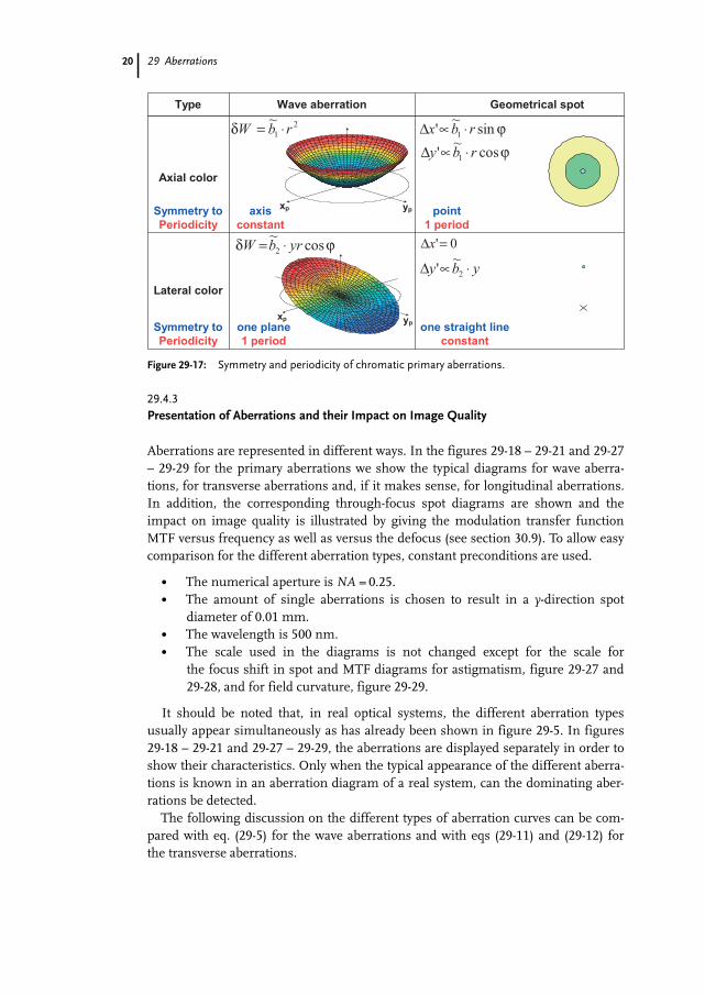
29.4.2Symmetry and Periodicity Properties

Often it is helpful to investigate symmetry and periodicity properties of the singleaberration type when analyzing the total aberrations of an optical system. This mayhelp to identify the dominating aberrations. For these considerations the fielddependence of the aberrations does not play a role. In figure 29-16 (primary mono-chromatic aberrations) and figure 29-17 (primary chromatic aberrations) symmetryand periodicity is shown for the wave aberrations as well as for the transverse aberra-tions. Three different types of symmetry occur:

1. Rotational symmetry with reference to an axis and to a point, respectively.Spherical aberration, field curvature and axial chromatic aberration all exhibitthis type of symmetry.

2. Mirror symmetry with reference to two planes and to two straight lines,respectively. This produces the appearance of astigmatism.

3. Mirror symmetry with reference to one plane and to one straight line, respec-tively. Coma and lateral chromatic aberration possess this type of symmetry.

The periodicity is defined as the period of the aberration for a single ray, while thepupil coordinates of this ray move through a concentric circle in the pupil. Thatmeans r = constant and � = 0 – 2� , keeping the field variable constant. It is impor-tant to note that wave aberrations and transverse aberrations show the same symme-try but different periodicity. For our treatment of the transverse aberrations in fig-ures 29-16 and 29-17 we use two circles in the pupil, first with a radius r (forinstance the maximum pupil radius) and second with radius r/2. In figures 29-16and 29-17 the spot diagrams for these rays are shown. The proportional relation-ships given for the transverse aberrations and the corresponding figures are gener-ated from eqs (29-15) and (29-16) by suppressing the constants.

It should be mentioned that the identification of aberrations by this method,which is based on symmetry properties, is not quite trouble-free. With higher orderaberrations new types of aberration show up and exhibit symmetry properties whichdo not correspond completely to the above results for the primary aberrations. Forexample when regarding fifth-order aberrations (see section 29.6.1) the so-called ob-lique spherical aberration exhibits mirror symmetry with reference to two planes,see figure 29-46 .So, the fifth- order oblique spherical aberration has the same typeof symmetry as third-order astigmatism. But this inconsistency does not really causea problem if kept in mind.

18

29.4 Primary Aberrations

Type

ypxp

ypxp

ypxp

ypxp

ypxp

4

1 rcW ⋅=

ϕ⋅= cos3

2 yrcW

ϕ⋅= 222

3 cosrycW

22

4 rycW ⋅=

ϕ⋅= cos3

5 rycW

ϕ⋅∝∆ sin' 3

1 rcx

ϕ⋅∝∆ cos' 3

1 rcy

ϕ⋅∝∆ 2sin' 2

2 yrcx

0'=∆x

ϕ⋅∝∆ cos' 2

3 rycy

ϕ⋅∝∆ sin' 2

4 rycx

ϕ⋅∝∆ cos' 2

4 rycy

0'=∆x3

5' ycy ⋅∝∆

Spherical

aberration

Symmetry to

Periodicity

axis

constant

point

1 period

Wave aberration Geometrical spot

Coma

Astigmatism

Field

curvature

(sagittal)

Distortion

Symmetry to

Periodicity

Symmetry to

Periodicity

Symmetry to

Periodicity

Symmetry to

Periodicity

one plane

1 period

two planes

2 period

one plane

1 period

axis

constant

point

1 period

one straight line

constant

one straight line

2 periods

two straight lines

1 period

)2cos2('2

2ϕ+⋅⋅∝∆ yrcy

Figure 29-16: Symmetry and periodicity of monochromatic primary aberrations.

19

29 Aberrations

ypxp

ypxp

Axial color

Lateral color

Symmetry to

Periodicity

Symmetry to

Periodicity

one plane

1 period

axis

constant

point

1 period

one straight line

constant

Type Wave aberration Geometrical spot

2

1

~rbW ⋅=δ

ϕ⋅=δ cos~

2 yrbW

ϕ⋅∝∆ sin~

' 1 rbx

ϕ⋅∝∆ cos~

' 1 rby

0'=∆x

yby ⋅∝∆ 2

~'

Figure 29-17: Symmetry and periodicity of chromatic primary aberrations.

29.4.3Presentation of Aberrations and their Impact on Image Quality

Aberrations are represented in different ways. In the figures 29-18 – 29-21 and 29-27– 29-29 for the primary aberrations we show the typical diagrams for wave aberra-tions, for transverse aberrations and, if it makes sense, for longitudinal aberrations.In addition, the corresponding through-focus spot diagrams are shown and theimpact on image quality is illustrated by giving the modulation transfer functionMTF versus frequency as well as versus the defocus (see section 30.9). To allow easycomparison for the different aberration types, constant preconditions are used.

� The numerical aperture is NA = 0.25.� The amount of single aberrations is chosen to result in a y-direction spot

diameter of 0.01 mm.� The wavelength is 500 nm.� The scale used in the diagrams is not changed except for the scale for

the focus shift in spot and MTF diagrams for astigmatism, figure 29-27 and29-28, and for field curvature, figure 29-29.

It should be noted that, in real optical systems, the different aberration typesusually appear simultaneously as has already been shown in figure 29-5. In figures29-18 – 29-21 and 29-27 – 29-29, the aberrations are displayed separately in order toshow their characteristics. Only when the typical appearance of the different aberra-tions is known in an aberration diagram of a real system, can the dominating aber-rations be detected.

The following discussion on the different types of aberration curves can be com-pared with eq. (29-5) for the wave aberrations and with eqs (29-11) and (29-12) forthe transverse aberrations.

20


Spherical aberrationAs shown in figure 29-18, for spherical aberration, the wave aberration curves are offourth power, so the transverse aberration curves are third-power polynomials.Spherical aberration is the only aberration for which the aberrations from the tan-gential and sagittal pupil section are identical. In the given example the sphericalaberration is under-corrected, which means that the upper marginal ray hits the axisin front of the paraxial image and so the intersection height in the paraxial imageplane is negative. Spherical aberration with the opposite sign is called over-cor-rected. From the through-focus analysis in the spot diagrams, as well as in the MTF,it can be seen that the best image quality is obtained not at the paraxial image planebut at an inward defocused position. Figure 29-19 represents the same sphericalaberration but focused to get the maximum MTF. Because of the defocusing in the

Wave aberration

tangential sagittal

λ2λ2

Primary spherical aberration at paraxial focus

Transverse ray aberration y′∆ x′∆ y′∆

Pupil: y-section x-section x-section

0.01 mm 0.01 mm 0.01 mm

Geometrical spot through

focus

0.0

2 m

m

Modulation Transfer Function MTF

MTF at paraxial focus MTF through focus for 100 cycles per mm

1

0

0.5

0 100 200cyc/mm z/mm

1

0

0.5

-0.02 0.020.0

z/mm-0.02 0.020.0-0.01 0.01

Figure 29-18: Spherical aberration at paraxial focus.

21

29 Aberrations22

Wave aberrationtangential sagittal

λ2λ2

Primary spherical aberration with compensating defocus

y′∆ x′∆ y′∆


0.01 mm 0.01 mm 0.01 mm

Transverse ray aberration


focus

0.0

2 m

m



z/mm-0.02 0.020.0-0.01 0.01

1

0

0.5


1

0

0.5

0.020.0-0.02

Figure 29-19: Spherical aberration of figure 29-18 with compensating defocus.

Longitudinal spherical aberration

0.02-0.02 0.0

aperture

'∆0.020.0-0.02

'∆

aperture

At paraxial focus With balancing defocus

z

Figure 29-20: Longitudinal aberration according to figures 29-18 and 29-19.


wave aberration curves, a second-power term is added and in the transverse aberra-tion curves this is a linear term. These additional terms balance the aberrations aswell as possible. In figure 29-20 the corresponding longitudinal aberrations are pre-sented. In this diagram the amount of balancing defocus can be clearly seen.

Coma

For primary coma it is typical that the wave aberration is zero for the sagittal section,see figure 29-21. In the tangential section the wave aberration is a third-power poly-nomial, so the transverse aberration is a second-power polynomial. A characteristic

Wave aberration

tangential sagittal

λ2λ2

Primary coma

Transverse ray aberrationy′∆ x′∆ y′∆


0.01 mm 0.01 mm 0.01 mm


focus

0.0

2 m

m



tangential

sagittal

tangential

sagittal

z/mm

-0.02 0.020.0-0.01 0.01

1

0

0.5


1

0

0.5

0.020.0-0.02

Figure 29-21: Coma.

23

29 Aberrations

property of the coma can be seen in the transverse aberration of rays in the sagittalpupil section where the x-component is zero while the y-component, representingthe sagittal coma (the coma from the sagittal pupil section), is similar to the y-com-ponent from the tangential pupil section, representing the tangential coma. Actuallythe sagittal coma is one-third of the tangential coma. It is interesting to note thatcoma is the only aberration which possesses contributions in the y-component fromthe sagittal section. This is an important feature when the transverse aberrations ofa real system which incorporates different aberration types are analyzed. The y-com-ponent from the sagittal section always shows the pure sagittal coma and no otheraberrations. On the other hand, in the usual representation of the transverse aberra-tions from the sagittal pupil section, only the x-component is shown while they-component is disabled. From through-focus analysis with help of spot diagramsand also the through-focus MTF, it is obvious that any defocus cannot improve theimaging. A further interesting property of coma can be seen from the through-focusMTF. In spite of the different sizes of the through-focus spot diagrams, the tangen-tial MTF (resolution in the y-direction) is almost constant over a certain defocusrange, while the sagittal MTF (resolution in the x-direction) shows a clear maximumat the focus with the smallest spot diagram.

As can be seen in figures 29-16 and 29-21, coma has the most complex spot dia-gram. Figure 29-22 demonstrates the geometrical coma spot in a three-dimensionalarrangement. The quantities “tangential coma” (from the chief ray intersectionpoint C to the tangential ray intersection point T) and “sagittal coma” (from the chiefray intersection point C to the sagittal ray intersection point S) are illustrated in thisfigure.

chief ray

sagittal ray

sagittal ray

tangential ray

tangential ray y'

x'

xp

yp

C

S

T

CT

tangential coma

CS

sagittal coma

C

S

T

Figure 29-22: Geometric spot for primary coma.

24


Due to the term 2� in eqs (29-15) and (29-16) for the transverse aberrations � x′and � y′ rays running through a concentric circle with radius r in the pupil, form acircle in the image with a radius proportional to r2 and the image circle is decenteredwith respect to the chief ray by a factor which is also proportional to r2. Figure 29-23is a schematic illustration of the ray path in a simple two- dimensional configurationas calculated from eqs (29-15) and (29-16).

Pupil Image

Figure 29-23: Schematic ray path for primary coma.

Depending on the sign of the coefficient c2 in eqs (29-5), (29-8), and (29-11) –(29-16), the coma is designated either as an outer or as an inner coma. In figure29-22 an outer coma is shown. All rays have image intersection points which have alarger distance to the image center than does the intersection point of the chief ray.Loosely speaking, the coma is driven outwards. In the opposite case when the aber-ration is driven inwards, it is designated as inner coma. In figure 29-24 outer andinner coma are shown schematically in one diagram.

x'

y'

inner

coma

outer

coma

optical

axis

Figure 29-24: Outer and inner coma.

25

29 Aberrations

Figure 29-25 represents an example of outer coma but in this figure the purelygeometrical spot is not shown but instead the physical intensity distribution is giv-en. The rotational symmetry with respect to the optical axis, the image center, is evi-dent.

Coma as ray aberration is usually understood as transverse aberration. Neverthe-less, sometimes it may be convenient to interpret coma as a longitudinal aberration:

y’

x’

Figure 29-25: Symmetry and intensity of coma.

chief ray

upper coma ray

lower coma ray

lows'

reference

image plane

optical

system

last

surface

tangential

coma

(transverse)

ups'

Figure 29-26: Definition of longitudinal coma.

26


� s′coma �s′up � s′low

2. (29-20)

Figure 29-26 is a sketch illustrating the definition for longitudinal coma, which isdetermined by the intersection points of the upper and lower coma ray with thechief ray. The upper and lower coma rays are also called meridional or tangentialcoma rays.

Astigmatism and Field Curvature

As shown in figures 29-27 and 29-28, astigmatism corresponds to a difference in thefocus position for the sagittal and tangential pupil section. In figure 29-27 the focus

Wave aberration

tangential sagittal

λ2λ2

Primary astigmatism at sagittal focus

Transverse ray aberration y′∆ x′∆ y′∆


0.01 mm 0.01 mm 0.01 mm




focus

0.0

2 m

m

sagittal

tangential

tangential

sagittal

z/mm-0.04 0.040.0-0.02 0.02

1

0

0.5

0 100 200cyc/mm /mz m

1

0

0.5

0.040.0-0.04

Figure 29-27: Astigmatism at sagittal focus.

27

29 Aberrations

is set to the sagittal image, as it is calculated in eqs (29-15) and (29-16). In figure 29-28 the mid-position between the sagittal and tangential focus is chosen as the receiv-ing image plane. In general this is of course only possible for a chosen imageheight. Figure 29-29 summarizes three cases: the paraxial image plane, the imageplane at the sagittal focus for maximum field, and the image plane at medial focusfor maximum field.

Wave aberration

tangential sagittal

λ2λ2

Primary astigmatism at medial focus

Transverse ray aberrationy′∆ x′∆ y ′∆


0.01 mm 0.01 mm 0.01 mm



sagittaltangential

tangentialsagittal

1

0

0.5


1

0

0.5

0.040.0-0.04


focus

0.0

2m

m

z/mm-0.04 0.040.0-0.02 0.02

Figure 29-28: Astigmatism of figure 29-27 with compensating defocus.

28


fieldfield field

Paraxial focus Sagittal focus Medial focus

Longitudinal

Astigmatism, sagittal and tangential field curvature

Figure 29-29: Sagittal and tangential field curvature as longitudinal aberration.

As shown in figure 29-29, the field dependence of the longitudinal sagittal andtangential field curvature is of second power. The astigmatism is defined as thelongitudinal distance (parallel to the z-axis of the optical system) of the tangentialfield measured from the sagittal field. A further discussion of astigmatism, sagittaland tangential field curvatures, and Petzval curvature follows in the next paragraph,when the Seidel sums are introduced.

29.4.4Calculation of the Seidel Sums

According to table 29-1 the coefficients c1 to c5 represent the amount of primaryaberrations. These coefficients depend on the system parameters (radii, separations,materials) and in addition they may depend on the position of the object as well asthe position of the aperture stop. There are different sets of formulae to calculate theprimary aberration coefficients for a given system. We will use the simplest formulaset which also provide a clear insight into how the single aberrations depend on thedifferent parameters. But instead of calculating the coefficients c1 to c5 used in themathematical derivation of the power series, we will define a new set of coefficients,the so-called Seidel sums: SI, SII, SIII, SIV, and SV which also represent the amountof primary aberrations. The relation between the ci-coefficients and the S-coeffi-cients will be given later. To make the equations as simple as possible the followingparaxial quantities are defined for each surface of the system:

A � n�hc � u� � n � i � n′ � i′ (29-21)

�A � n��hc � �u� � n ��i � n′ ��i′ (29-22)

All quantities with a bar refer to the chief ray, the corresponding quantities withoutthe bar refer to the marginal ray. As usual n is the refractive index, i is the paraxial

29

29 Aberrations

incidence angle, u is the paraxial convergence angle, h is the paraxial incidenceheight at the surface, and c is the surface curvature. In figure 29-30 these paraxialquantities are shown for the marginal ray. Actually all these quantities have an indexwhich indicates the surface number, but here the index is suppressed. So A and �Aare the refraction invariants at the chosen surface.

u u'

i

i’h

n'n

r=1/c

Figure 29-30: Quantities used to calculate the refraction invariant.

The increment on refraction is designated by � �x� � x ′ � x. H is the Lagrangeinvariant containing the aperture and the maximum field, see section 2.5, Invar-iants. For the chromatic aberrations we have the refractive index n for the referencewavelength �and the refractive index n + �n for the wavelength �+ ��.

Based on these quantities, which are to be calculated by tracing two paraxial rays,namely the marginal ray for full aperture and the chief ray for the maximum field,the following expressions define the Seidel sums [29-2].

Spherical aberration SI � ��

A2 � h � �un

� �(29-23)

Coma SII � ��

�AA � h � �un

� �(29-24)

Astigmatism SIII � ��

�A2 � h � �un

� �(29-25)

Petzval SIV � ��

H2 � c � �1n

� (29-26)

Distortion SV � �� A3

A� h � �

un

� ��

�AA� H2 � c � �

1n

� �(29-27)

Axial color CI ��

A � h � ��nn

� (29-28)

Lateral color CII ��

�A � h � ��nn

� (29-29)

where the summation is taken over all surfaces of the system.Concerning the chromatic aberrations given in eqs (29-28) and (29-29) it must be

mentioned that the height h and the refraction invariants A and �A actually dependon the wavelength. As for most imaging systems the influence of this dependence issmall, h, A and �A are calculated only for the primary wavelength and the wavelength

30


dependence is neglected, as it is done in eqs (29-28) and (29-29). A more compre-hensive treatment is given by Wynne [29-3].

It should be mentioned that also for reflecting mirror surfaces the formulae (29-23) to (29-29) should be applied. As usual for a reflective surface the refractiveindices are set to n′ � �n. Looking at eqs (29-28) and (29-29) it is evident that reflect-ing surfaces possess zero color aberrations. From eqs (29-23) – (29-27) for mono-chromatic aberrations, eq. (29-26) for the Petzval curvature becomes a special casedue to the term � 1�n� �. In fact, mirror surfaces will play a notable role in the correc-tion of the Petzval curvature, see chapter 31, Correction of Aberrations.

The Seidel sums SI – SV and CI – CII are calculated for the maximum apertureand the maximum field. So, to express the wave aberration (29-8) in terms of theseSeidel sums, the pupil coordinate r and the field coordinate y must be redefined asrelative and dimensionless coordinates:

� � rr max

�

� � yy max

�(29-30)

With these quantities the total primary monochromatic wave aberration reads

W�� 18

SI�4 � 1

2SII��

3 cos�� 12

SIII�2�2 cos 2�� 1

4SIII � SIV� ��2�2 � 1

2SV�3� cos��

(29-31)

The constants 1/8 , 1/2 , etc. in (29-31) are a consequence of the common definitionof the Seidel sums (29-23) – (29-29). As can be seen by a comparison of (29-8) and(29-31) there is a correspondence between the c-coefficients in the power seriesexpansion and the Seidel coefficients. Table 29-2 gives an overview.

Table 29-2: Wave aberration expansions: power series and corresponding Seidel coefficients.

Aberration Power series coefficientDimension unit: (length)–3

Seidel coefficientDimension unit: (length)

Spherical aberration c1 SI

Coma c2 SII

Astigmatism (half astigmatic difference) c3 SIII

Sagittal field c4 SIII + SIV

Tangential field c4 + 2c3 3SIII + SIV

Petzval field c4 – c3 SIV

Distortion c5 SV

29 Aberrations

It should be noted that there is an important difference in the dimension units ofthe c-coefficients and the S-coefficients. While the S-coefficients have the dimensionof length (due to h in eqs (29-23) – (29-29)) the c-coefficients have the dimension of(length)–3.

From table 29-2 the relations between the aberrations of astigmatism, sagittalfield curvature, tangential field curvature, and Petzval field curvature can clearly beseen. These four aberrations are calculated from two coefficients, either c3 and c4 orSIII and SIV . On the other hand, when any two of these four aberrations are known,the other two can de determined. This can be seen from table 29-2 as well as fromeqs (29-32) and (29-33). When the astigmatism is zero, SIII = 0 , the tangential andthe sagittal field coincide with the Petzval field and SIV represents the curved imageplane. That is the only situation when there is a typical image formation at the loca-tion of the Petzval field. When the astigmatism is not zero, the Petzval field justserves as a basis to determine the sagittal and tangential field and SIV = 0 is a pre-condition for a flat field. As seen from eqs (29-23) – (29-29) the Petzval field SIV isthe only Seidel coefficient which is completely independent of the ray quantities u,h, and A from the marginal as well as �h and �A from the chief ray, so SIV is indepen-dent of object, image, and stop position. It is only the surface curvatures of the sys-tem and the refractive indices which determine the Petzval field SIV. The Lagrangeinvariant H appears as a factor because the given formulation of the Seidel coeffi-cients are related to the full aperture and the maximum field.

PST

field∆s'ast

∆s'pet

∆s'tan

∆s'sag

∆ s’

Figure 29-31: Longitudinal aberrations related to the Petzval,sagittal, and tangential field curvatures.

32


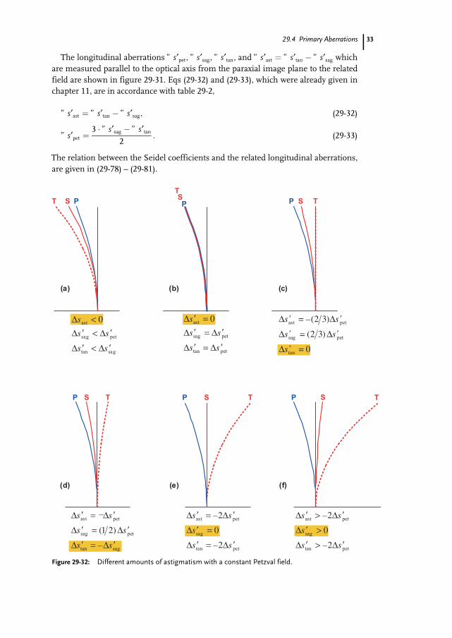
The longitudinal aberrations � s′pet, � s′sag, � s′tan, and � s′ast � � s′tan � � s′sag whichare measured parallel to the optical axis from the paraxial image plane to the relatedfield are shown in figure 29-31. Eqs (29-32) and (29-33), which were already given inchapter 11, are in accordance with table 29-2,

� s′ast � � s′tan � � s′sag� (29-32)

� s′pet �3 � � s′sag � � s′tan

2� (29-33)

The relation between the Seidel coefficients and the related longitudinal aberrations,are given in (29-78) – (29-81).

TP S S TPSP T

sagtan

petsag

petast

ss

ss

ss

'∆–='∆

'∆='∆

'∆='∆)21(

pettan

sag

petast

ss

s

ss

'∆–='∆

='∆

' –='∆

2

0

2∆

pettan

sag

petast

ss

s

ss

'∆–>'∆

>'∆

'∆–>'∆

2

0

2

(d) (e) (f)

T PS

T

TP S

(b) (c)

PS

(a)

sagtan

petsag

ast

ss

ss

s

'∆<'∆

'∆<'∆< ∆ 0

pettan

petsag

ast

ss

ss

s

'∆='∆

'∆='∆='∆ 0

0

)32(

)32(

='∆

'∆='∆

'∆–='∆

tan

petsag

petast

s

ss

ss

–

Figure 29-32: Different amounts of astigmatism with a constant Petzval field.

29 Aberrations

In figure 29-32 a constant, inwardly curved Petzval field is assumed and the sagit-tal and tangential fields for different amounts of astigmatism are shown. In parti-tion (a) a typical uncorrected situation with some negative astigmatism is shown. Inpartition (b) the astigmatism is corrected to zero, but the image is not flat, but it iscurved according to the Petzval field. Partition (c) represents a special situation, thetangential field is flat, but due to the negative Petzval field, which is held constantfor all partitions, the sagittal field is negative and so there is some positive astigma-tism. Partition (d) shows another specific situation when the sagittal field is negativeand the tangential field is positive with the same absolute value. So, the mediumfield between the sagittal and tangential field is flat. This can be seen as a possiblecompromise when optimizing a system, if the Petzval field cannot be furtherreduced. In fact the astigmatism is larger than in partition (c), but in (c) the inter-mediate image between the sagittal and tangential is curved. The next partition (e)shows a flat sagittal field. The disadvantage of this situation, compared with the flattangential field in (c), is the relatively large astigmatism. Partition (f) shows an evenlarger astigmatism with the result that both the sagittal and tangential fields are pos-itive.

There is an interesting systematic in the formulae for the Seidel sums (29-23) –(29-29) which can easily be seen when the single summands, the so-called surfacecontributions, are designated by square brackets in the following way:

SI ��

�

sI� �� (29-34)

SII ��

�

sII� ��

�

�AA

sI� �� (29-35)

SIII ��

�

sIII� ��

�

�AA

sII� �� (29-36)

SIV ��

�

sIV� �� (29-37)

SV ��

�

sV� ��

�

�AA�

sIII� �� sIV� ��

(29-38)

CI ��

�

cI� �� (29-39)

CII ��

�

cII� ��

�

�AA

cI� �� (29-40)

A graphical presentation of the single surface contributions can be very helpful inorder to get a specific insight as to which surfaces contribute which amount of thevarious aberrations. As an example, figure 29-33 shows a cross-section of a retrofo-cus-type photographic lens and figure 29-34 gives the associated surface contribu-tions for the Seidel aberrations in a bar diagram [29-4]. It should be noticed that thescale for the various aberrations is different.

34


1

23 4

5

6 8 9

10

7

Retrofocus F/2.8

Field: w=37°

Figure 29-33: Retrofocus-type photographic lens, modified from [29-5].

SISpherical Aberration

SIIComa

-200

0

200

-1000

0

1000

-2000

0

2000

-1000

0

1000

-100

0

150

-400

0

600

-6000

0

6000

SIIIAstigmatism

SIVPetzval field curvature

SVDistortion

CIAxial color

CIILateral color

Surface 1 2 3 4 5 6 7 8 9 10 Sum

Figure 29-34: Bar diagram showing Seidel sums and relatedsurface contributions for the lens in figure 29-33.

35

29 Aberrations36

It can be seen in figure 29-34 that, for all aberrations, the Seidel sums in the lastcolumn are essentially smaller than the main surface contributions, which partlycancel each other. Further, in combination with figure 29-33 it can be seen that rela-tively large surface contributions arise at surfaces where the associated rays havelarge incidence angles. For instance: regarding spherical aberration, the marginalray exhibits relatively large incidence angles at surfaces 5 and 10, while for distortionthe chief ray exhibits large incidence angles at surfaces 4, 6, and 7.

When correcting the aberrations of an optical system it is usually not enough toobtain small aberrations for the whole system, but the single surface contributionsshould also be small, so that the system is not too sensitive to manufacturing toler-ances. See chapter 35 for a further discussion.

29.4.5Stop Shift Formulae

As can be seen from eqs (29-23) – (29-29) SI is completely independent of the chiefray, which is expected, because SI represents spherical aberration. SIV is dependenton H , the Lagrange invariant and so SIV depends on the maximum aperture andthe maximum field, but SIV is independent of the marginal ray quantities h, u, A,and also independent of the chief ray quantities �A. The Seidel sums which dependon the chief ray are: SII, SIII, and SV. As the chief ray is determined by the stop posi-tion, SII, SIII, and SV must change when the stop position in the system is changed.There are so-called stop shift formulae which are very simple and provide an inter-esting insight into the impact of shifting the stop. These stop shifts are specified ina way that the marginal ray does not change, that means that while shifting the stopposition, the size of the stop is adapted to the marginal ray as shown in figure 29-35.

old position

new position

old chief ray

new chief ray

oldh

newh

Figure 29-35: Stop shift.


The stop position can be characterized at each surface by the so-called Seideleccentricity

E ��hh

, (29-41)

which indicates the eccentricity of the oblique ray bundle relative to the axial bundle.The main advantage in describing the stop position at each surface with this para-meter E is the handling of a stop shift. When the stop is shifted a certain distance,as shown in figure 29-35, at a chosen surface the chief ray intersection heightschange from �hold to �hnew and the Seidel eccentricity is changed by the amount

�E ��hnew � �hold

h. (29-42)

It transpires that, for a given stop shift, this quantity �E has the same value for allsurfaces of the system. Thus �E indicates a certain stop shift.

Let S�I to S�

V and C�I and C�

II indicate the Seidel sums after a stop shift representedby �E, then there is a very simple and instructive set of formulae describing thetransformation of the Seidel sums, the so-called stop shift formulae:

S�I � SI (29-43)

S�II � SII � �E � SI (29-44)

S�III � SIII � �E � SII � �E2 � SI (29-45)

S�IV � SIV (29-46)

S�V � SV � �E � 3SIII � SIV� � � 3�E2 � SII � �E3 � SI (29-47)

C�I � CI (29-48)

C�II � CII � �E � CI (29-49)

From these formulae, for instance, it can be seen that with a stop shift the coma(SII) changes in the same rate as the spherical aberration (SI) occurs in the system.So, more or less theoretically, if SI is unequal to zero, then the coma can be madezero by the appropriate localization of the stop position. On the other hand thecoma will be unaffected by a stop shift if the spherical aberration is zero. Such typesof statements based on the stop shift formulae (29-43) – (29-49) are valid of courseonly for primary aberrations. With higher order aberrations equivalent statementswould be much more complicated. Corresponding formulae are therefore not inuse.

37

29 Aberrations

29.4.6Several Aberration Expressions from the Seidel Sums

Based on the Seidel sums SI – SV and CI – CII as given in eqs (29-23) – (29-29) allprimary aberrations of a given optical system can be calculated.

There are in particular: wave aberrations, transverse aberrations, angular aberra-tions, fractional expressions, and all field curvatures.

In several of these expressions u′ designates the image side convergence angle(maximum aperture) and n′ is the refractive index in the image space. The tables29-3 – 29-8 summarize these results.

Table 29-3: Wave aberrations based on Seidel sums.

Primary wave aberrations

Spherical aberration Wspherical �SI

8�4 (29-50)

Coma Wcoma �SII

2��3 cos� (29-51)

Astigmatism Wast �SIII

2�2�2 cos 2� (29-52)

Petzval field Wpetzval �SIV

4�2�2 (29-53)

Sagittal field Wsag �SIII � SIV

4�2�2 (29-54)

Tangential field Wtan � 3SIII � SIV

4�2�2 (29-55)

Distortion Wdist �SV

2�3� cos� (29-56)

Axial color Wac �CI

2�2 (29-57)

Lateral color Wlc � CII�� cos� (29-58)

38


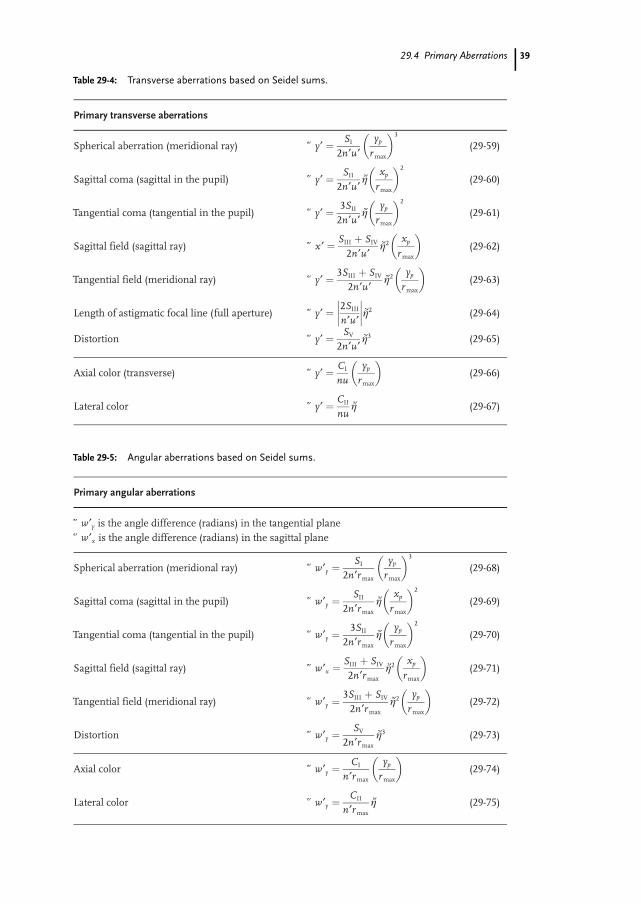
Table 29-4: Transverse aberrations based on Seidel sums.

Primary transverse aberrations

Spherical aberration (meridional ray) � y′ � SI

2n′u′yp

r max

� 3

(29-59)

Sagittal coma (sagittal in the pupil) � y′ � SII

2n′u′�

xp

r max

� 2

(29-60)

Tangential coma (tangential in the pupil) � y′ � 3SII

2n′u′�

yp

r max

� 2

(29-61)

Sagittal field (sagittal ray) � x ′ � SIII � SIV

2n′u′�2 xp

r max

� (29-62)

Tangential field (meridional ray) � y′ � 3SIII � SIV

2n′u′�2 yp

r max

� (29-63)

Length of astigmatic focal line (full aperture) � y′ � 2SIII

n′u′

��2 (29-64)

Distortion � y′ � SV

2n′u′�3 (29-65)

Axial color (transverse) � y′ � CI

nu

yp

r max

� (29-66)

Lateral color � y′ � CII

nu� (29-67)

Table 29-5: Angular aberrations based on Seidel sums.

Primary angular aberrations

� w ′y is the angle difference (radians) in the tangential plane� w ′x is the angle difference (radians) in the sagittal plane

Spherical aberration (meridional ray) � w ′y �SI

2n′r max

yp

r max

� 3

(29-68)

Sagittal coma (sagittal in the pupil) � w ′y �SII

2n′r max

�xp

r max

� 2

(29-69)

Tangential coma (tangential in the pupil) � w ′y �3SII

2n′r max

�yp

r max

� 2

(29-70)

Sagittal field (sagittal ray) � w ′x � SIII � SIV

2n′r max

�2 xp

r max

� (29-71)

Tangential field (meridional ray) � w ′y �3SIII � SIV

2n′r max

�2 yp

r max

� (29-72)

Distortion � w ′y �SV

2n′r max

�3 (29-73)

Axial color � w ′y �CI

n′r max

yp

r max

� (29-74)

Lateral color � w ′y �CII

n′r max

� (29-75)

29 Aberrations

Table 29-6: Longitudinal aberrations based on Seidel sums.

Primary longitudinal aberrations

Spherical aberration (meridional ray) � s′ � � SI

2n′u′2yp

r max

� 2

(29-76)

Coma � s′coma � � 3SII

2n′u′2�

yp

r max

� (29-77)

Sagittal field (Gaussian image to s-focus) � s′sag � �SIII � SIV

2n′u′2�2 (29-78)

Tangential field (Gaussian image to t-focus) � s′tan � � 3SIII � SIV

2n′u′2�2 (29-79)

Astigmatism (from s- to t-focus) � s′ast � � s′tan � � s′sag � � SIII

n′u′2�2 (29-80)

Petzval field (Gaussian image to Petzval) � s′pet � � SIV

2n′u′2�2 (29-81)

Axial color � s′ � � CI

n′u′2(29-82)

Table 29-7: Fractional aberrations based on Seidel sums.

Primary fractional aberrations

Fractional distortionSV

2n′u′y′ max

�2 � SV

2H�2 (29-83)

Fractional lateral colorCII

2n′u′y′ max

� CII

H(29-84)

Table 29-8: Field curvature aberrations based on Seidel sums.

Primary image surface curvatures

Sagittal field curvature csag � � SIII � SIV

n′u′2y′2max

� �n′�SIII � SIV�H2

(29-85)

Tangential field curvature c tan � � 3SIII � SIV

n′u′2y′2max

� �n′�3SIII � SIV�H2

(29-86)

Petzval field cpet � � SIV

n′u′2y′2max

� � n′SIV

H2(29-87)

40


29.4.7Thin Lens Aberrations

In eqs (29-23) – (29-29) the surface contributions of the primary aberrations aregiven. Often it is advantageous to work with the contributions of a thin lens. Theidealization of zero lens thickness leads to a considerable simplification of the for-mulae. Although there are no thin lenses in the real world, the results from the thinlens theory hold in many cases to a good approximation. To get the thin lens contri-butions, two surface summands of eqs (29-23) – (29-29) must be considered andshould be expressed in terms of the parameters of a thin lens. These thin lensparameters are the bending parameter X and the position or conjugate or magnifica-tion parameter M (see sections 10.1.1 Bending of Lenses, and 10.1.2 Position Para-meter),

X � c1 � c2

c1 � c2

(29-88)

where c1 and c2 are the curvatures of the two surfaces, and

M � u2 ′ � u1

u2 ′ � u1

(29-89)

where u1 and u2′ are the angles of the paraxial marginal ray before and after thelens, respectively. Let n be the refractive index of the lens, then the refractive powerreads

� � �n � 1��c1 � c2�. (29-90)

For the chromatic aberrations we will use the Abbe number, which in this context isdefined as

� � n � 1�n

. (29-91)

To get the essential information from the thin lens contribution formulae, it is suffi-cient to assume the stop at the lens, so that the incidence height of the chief ray iszero. If the influence of a remote stop position is to be incorporated, it is easy toapply the stop shift formulae (29-43) – (29-49).

With these parameters the primary aberrations of the thin lens (stop at the lens)are:

SI �� 3h4

43n � 2

nM2 � 4n � 4

�n � 1�n XM � n � 2

�n � 1�2nX2 � n2

�n � 1�2

� �(29-92)

SII �H� 2h2

22n � 1

nM � n � 1

�n � 1�n X

� (29-93)

SIII � H2� (29-94)

41

29 Aberrations42

SIV � H2�n

(29-95)

SV � 0 (29-96)

CI �� h2

�(29-97)

CII � 0. (29-98)

Again, to calculate the Seidel sums, the paraxial rays for both maximum apertureand maximum field must be used. As the Lagrange invariant H contains both theaperture and the field size as linear factors, the dependence of the Seidel contribu-tions on the aperture and field can easily be checked.

From eq. (29-92) it can be seen that the spherical aberration SI depends quadrati-cally on both M, the conjugate parameter, and on X, the bending parameter. In fig-ures 29-36, 29-37 and 29-38 this behavior is illustrated. In figure 29-36 the sphericalaberration is shown as a function of the bending parameter X for several conjugateparameters M and for a refractive index n = 1.5. In figures 29-37 and 29-38 contourplots and a section for M = 3 are shown for two different refractive indices, for n= 1.5and for n= 1.9. With the help of the lines for zero spherical aberration it can be seenthat, in the range of real imaging (neither virtual object nor image) represented by–1 ≤ M ≤ +1, the spherical aberration is positive, which implies under-correction.Only for extremely large conjugate parameters M and the appropriate bending pa-rameters X can the spherical aberration vanish or even exhibit over-correction. Fig-ure 29-38 shows that for the high refractive index n = 1.9 the smallest M whichallows approximately zero spherical aberration is M = 3, the appropriate bendingparameter is then X = 4. Because of the symmetry of the eq. (29-92) the sphericalaberration is also very close to zero when changing the sign of both M and X, i. e.for M = –3 and X = –4.

20

40

60

-7 -6 -5 -4 -3 -2 -1 0 1 2 3 4 5 6 7

X

M=-6 M=6M=-3 M=3

M=0

Spherical

Aberration

Figure 29-36: Spherical aberration,4

� 3h4SI of a thin lens as a

function of the bending parameter X and the conjugate para-meter M. The refractive index is n = 1.5.


scale

-10

0

+10

+20

+30

+40

X

M

SI=0

n = 1.5

range of realimaging

SI=0

0 2 4 6 8-2-4-6-8

0

2

4

6

8

-2

-4

-6

-8

section M = 3

0

42

40

0

20M = 3

Sph.

Aberr

X-1 < M < 1




scale

-10

0

+10

+20

+30

+40

X

M

SI=0

n = 1.9

range of real

imaging

SI=0

0 2 4 6 8-2-4-6-8

0

2

4

6

8

-2

-4

-6

-8

section M = 3

0

4 8

40

0

20

-1 < M < 1

Sph.

Aberr

X

M = 3




43

29 Aberrations

Virtual image Virtual object

X=4.0 M=3.0M=-3.0 X=-4.0

X=3.3 M=4.6M=-4.6 X=-3.3

n

1.5

1.9O'

OO'O' O

O OO'

Figure 29-39: Single lens with zero spherical aberration withminimum M� � for n = 1.5 and for n = 1.9.

In figure 29-39 it is demonstrated again that the condition for zero primary spher-ical aberration for a single lens is possible only in virtual imaging and for a stronglymeniscus shaped lens. For the refractive indices n = 1.5 and n = 1.9 the minimumvalues for the absolute conjugate parameter M� � which allow zero spherical aberra-tion are used, together with the appropriate lens bending X. In fact eq. (29-92) isbased on thin lenses but in figure 29-39 finite lens thicknesses are introduced formore clarity. On the other hand these thicknesses have low influence and can oftenbe neglected.

For a given conjugate parameter M the bending parameter X, which delivers theminimum spherical aberration can be calculated from eq. (29-92):

Xsph min � 2 n2 � 1� �n � 2

M. (29-99)

A special application of this formula yields the optimal bending of a single thinlens, for the object at infinity, which means the incoming light is collimated and theconjugate parameter is M = +1. A lens with this bending parameter,

X min � 2�n2 � 1�n � 2

, (29-100)

is called the lens with the optimal bending with respect to spherical aberration.According to eq. (29-100) the optimal bending depends on the refractive index n. Forn = 1.686 one gets X = 1, the plano-convex lens with the convex surface on the objectside. For indices n <1.686 the optimal bending shape is biconvex and for n >1.686the best form is a meniscus shape.

44

29.5 Pupil Aberrations 45

Eq. (29-93) for SII shows that coma depends linearly on the conjugate parameterM as well as on the bending parameter X. So, for a lens, whatever the conjugateparameter may be, there is always a suitable bending

X � �2n � 1��n � 1��n � 1� M (29-101)

which makes the primary coma zero. If the stop is not at the lens, the contributionto coma due to the spherical aberration according to the stop shift formula (29-44)must also be taken in account.

From eqs (29-94)–(29-96) we see that astigmatism, Petzval curvature and distor-tion are independent of both the lens bending (X) and the conjugate position (M).But with a remote stop due to the contributions from spherical aberration and alsofrom coma, which take effect through the stop shift formulae (29-45) and (29-47),astigmatism and distortion are no longer independent of the lens bending (X) andof the conjugate position (M). The primary chromatic aberrations CI and CII arealways independent of both X and M.

29.5Pupil Aberrations

After the discussion of the influence of a stop shift on the primary aberrations inparagraph 29.4.5, it sounds reasonable to also investigate an object shift. Of coursein most optical designs an object shift does not have the relevance of a pupil shift but theobject shift is studied in order to obtain a better theoretical insight, [29-6], [29-7]. Thebest way of doing this is to exchange the function of the object and the pupil. More pre-cisely: rather than considering the imaging of the object onto the image through thepupil, the imaging of the entrance pupil onto the exit pupil through the object andimage are examined instead. In this process, as shown in figure 29-40 the

O O'

stop and

entrance pupil

optical system

exit pupil

objectimage

Object imaging Pupil imaging

Blue rays

Red rays

Marginal rays

Marginal raysChief rays

Chief rays

Figure 29-40: Object and pupil imaging.

29 Aberrations

marginal rays of the normal imaging become the chief rays of the pupil imagingand the chief rays of the normal imaging act as marginal rays in the pupil imaging.

In fact there is a complete dualism in object and pupil imaging. So all the givenformulae can be used for the pupil imaging to calculate pupil aberrations, providedthat the quantities based on the marginal ray such as u, A, h and so on are replacedby their corresponding quantities �u� �A� �h based on the chief ray, and vice versa. Theseconsiderations are not really difficult but lengthy and – much more important – theresults are usually not in use. Nevertheless there are some interesting conclusionsfrom this pupil aberration theory which should be quoted here:

� Wave aberration power series expansionPrimary spherical pupil aberration only depends on the field coordinate. As awave aberration it depends on the 4th power in the field coordinate, whichcorresponds to the term c6y4 in the power series expansion (29-5) for the waveaberration. This term was set to zero, because at that time only image aberra-tions were considered. So, all terms in the power series expansion haveindeed meaning, if it is not only the image aberrations but also the pupilaberrations that are taken into account.

� DistortionThe spherical pupil aberration plays a part when, for normal imaging, thedistortion is investigated independently of the object and corresponding im-age shift. In fact, the change in distortion is proportional to the pupil spheri-cal aberration in the exit pupil. So, if the distortion is to be independent ofthe object position, then the spherical pupil aberration must be zero. Underthe precondition of zero spherical pupil aberration the distortion is zero ifthe so-called tangent condition [29-8] if fulfilled. The tangent condition reads

tan �U ′tan �U

� constant for all field angles �U and �U ′� (29-102)

� ObscurationWhen two parts of an interlinked optical system, for example, an objectiveand an eyepiece, are put together, both the field positions and the pupil posi-tions must be matched. In greater detail: the object plane of the eyepiece hasto match the image plane of the objective and the entrance pupil of the eye-piece has to match the exit pupil of the objective. When the parts to be com-bined are designed simultaneously this usually doesn’t represent a problem,but when they are designed independently, then pupil aberrations, in particu-lar, may frustrate the combination. A similar situation occurs with the combi-nation of an eyepiece and the eye of the observer. This case is actually morecritical, since the pupil of the eye is not really fixed. Particularly in wide-angleeyepieces, where the observer has to rotate the eye to look from one to theother end of the field of view. Due to this rotation the pupil of the eye takes adecentered position and, dependent on the size of the exit pupil of the eye-piece and the size of the eye pupil, this may result in a decreased image

46

29.5 Pupil Aberrations

illumination. If the eyepiece exhibits a strong spherical pupil aberration, thenthe decentered eye pupil may result in a partial obscuration of the imagefield. An example of a significant pupil aberration is given in figures 29-41 to29-43. Figure 29-41 shows an eyepiece with a rather large pupil aberration,together with an idealized eye. The curve of the transverse spherical pupilaberration is given in figure 29-42. Note the maximum values of about ± 4mm in the zone of the pupil. This large aberration is the reason for the ob-scuration increasing with the decentering of the eye pupil, as displayed infigure 29-43. When the pupil of the eye is decentered, the rays in the zone ofthe pupil are truncated first, as can be understood from the ray path in theinsert of figure 29-41. Therefore, the intensity first drops in a zonal region ofthe retina image. A certain area in the image even shows zero intensity. Ifhigh-quality imaging of the pupil of the instrument is required, then thedecentering would cause a uniform decrease in the intensity.

eyepiecelens and pupil of the eye

retina

caustic of the pupil image enlarged

instrument pupil

Figure 29-41: A ray path in the eyepiece with an idealized eye.The system suffers from a large spherical pupil aberration, seefigure 29-42. The ray caustic is also shown in an enlarged illus-tration.

47

29 Aberrations

y' ∆5 mm

yp

Figure 29-42: Spherical pupil aberration as a transverseaberration of the eyepiece in figure 29-41.

Figure 29-43: Illumination of the retina image for the systemshown in figure 29-41 with different values of the decentered eyepupil. The offset of the pupil causes a truncation of the ray bun-dles and therefore the intensity is locally decreased.

� Ray aimingPupil aberrations play a role in another field , which is more closely related topractical ray tracing than to image aberrations. In order to trace a selectedray, such as a marginal ray or a chief ray, through an optical system, then forfast ray tracing, the entrance pupil is very often used to aim the ray. As theentrance pupil is defined as the paraxial image of the aperture stop throughthat part of the system which is in front of the stop, it may occur that raysaimed towards the entrance pupil cannot pass through the system. This isdue to large pupil aberrations. An example is given in figure 29-44 (a), whichshows a wide-angle lens modified from [29-9] to demonstrate this effect.None of the rays from the maximum oblique bundle, when aimed towardsthe entrance pupil can pass through the lens. In such systems with large pu-pil aberrations the rays to be traced must be aimed towards the real aperturestop as shown in figure 29-44 (b). This is more time consuming but doessolve the problem.

48

29.5 Pupil Aberrations

a

Aperture

stopEntrance

pupil

Entrance beam

equal to axial beam

b

Aperture

stop

Entrance beam

larger than axial beam

Figure 29-44: Pupil aberration and ray aiming. (a) Ray aiming towardsthe paraxial entrance pupil; (b) ray aiming towards the aperture stop.

� IlluminationAs can be seen in figure 29-44 (b), when the rays are traced to the aperturestop, there is also an effect on the meridional bundle diameters. With in-creasing field angle the meridional bundle diameters also increase, which re-duces the illumination fall-off in the image. By further studying this effect itcan be shown that the increased entrance beam diameter in the oblique bun-dles is a consequence of pupil coma aberration: when imaging the aperturestop on the entrance pupil there is a considerable amount of outer coma.

� Petzval curvatureThe Seidel Petzval sum for usual and pupil imaging is identical. So the Petz-val curvature in the exit pupil, when assuming a flat entrance pupil, is thesame as in the image.

49

29 Aberrations

29.6High-order Aberrations

The primary or third-order aberrations discussed in section 29.4 represent the basicprinciples of aberration theory. In practice, already the secondary or fifth-order aber-rations are not usually used in complete detail to analyse the aberrations of an opti-cal system. As we will see in the next paragraph, the set of nine fifth-order aberra-tions contain new types of aberration, particularly with regard to the pupil or aper-ture dependence of the aberrations. Nevertheless, the main problem in lens designis to prevent or to correct all, including the higher-order aberrations. It is wellknown by the experienced optical designer that, during the optimization of an opti-cal system, the third-order aberrations are much more movable than the higher-order aberrations. So, if it is not possible to correct the aberrations to zero, the resultof the optimization is a balancing of third-order against higher-order aberrations ofthe same, or at least of a similar, type. In this view the amount of third-order aberra-tions is chosen to balance the uncorrectable higher-order aberrations. For this rea-son, in the next paragraph, the fifth-order aberrations are grouped together with therelated third-order aberrations.

29.6.1Fifth-order Aberrations

The terms containing the coefficients d1 to d9 in eqs (29-5) and (29-8) represent thenine secondary or fifth-order wave aberrations. In the following figures (29-45 –29-52) the pupil dependence of these fifth-order aberrations are arranged with therelated third-order types.

Primary, 3rd Order Secondary, 5th Order

Spherical Aberration

ypxp ypxp

4

1 rcW ⋅= 6

1 rdW ⋅=

Figure 29-45: Primary and secondary spherical aberration.

The primary spherical aberration is of 4th power in the aperture. The secondaryspherical aberration is of 6th power in the aperture. Higher power spherical aberra-tion is easy to detect. As an example, in figure 29-53, a microscope objective with atleast ninth-order spherical aberration is shown.

50

29.6 High-order Aberrations


Spherical Aberration

Oblique Spherical Aberration

ypxpypxp

4

1 rcW ⋅= ϕ⋅= 242

3 cosrydW 42

4 rydW ⋅=

ypxp

Figure 29-46: Primary and oblique spherical aberration.

The oblique spherical aberration (the sum of the d3 and d4 terms) is of 4th powerin aperture as is the primary spherical aberration. But the field dependence of theoblique spherical aberration is of 2nd power and due to the d3 term the amount ofwave aberration is different in the tangential and sagittal directions. In practical lensdesign the resulting component in the sagittal direction is often dominant and iscalled: the “oblique spherical sagittal aberration”. As mentioned in the discussionabout the symmetry properties of aberrations in section 29.4.2, the oblique sphericalaberration does not have rotational symmetry as does the third-order spherical aber-ration.


Coma

ypxp yp

xp

ϕ⋅= cos3

2 yrcW ϕ⋅= cos5

2 yrdW

Linear coma

Figure 29-47: Primary and secondary linear coma.

The designation “linear” coma describes the linear field dependence of this aber-ration. The higher power appears only in the pupil coordinate. It should be notedthat this higher-order aberration is included in the scope of the sine condition andthe “offence against the sine condition” just because it is linear in the field coordi-nate as discussed in section 29.8.1.

51

29 Aberrations52

Primary, 3rd Order

Elliptical coma

Coma

Secondary, 5th Order

ypxp yp

xp ypxp

ϕ⋅= cos3

2 yrcW ϕ⋅= cos33

5 rydW ϕ⋅= 333

6 cosrydW

Figure 29-48: Primary and elliptical coma.

The designation “elliptical” coma results from the appearance of the associatedtransverse aberration. The circles in the image spot shown in figure 29-23 for third-order coma, originating from concentric circles in the pupil, will change to ellipsesin the case of elliptical coma. The coefficient d6 controls the shape of the ellipses.An example analog to figure 29-23 is shown in figure 29-49.

sagittal

Pupil Image

tangential

chief

Figure 29-49: Schematic ray path for elliptical coma.


Astigmatism

ypxp ypxp

ϕ⋅= 222

3 cosrycW ϕ⋅= 224

7 cosrydW

Figure 29-50: Primary and secondary astigmatism.

29.6 High-order Aberrations


Field curvature (sagittal)

ypxp ypxp

22

4 rycW ⋅= 24

8 rydW ⋅=

Figure 29-51: Primary and secondary sagittal field curvature.

Fifth-order astigmatism and fifth-order field curvature as shown in figures 29-50and 29-51 are both easy to understand: it is just the field dependence which is offourth power instead of second power for the primary aberrations. As the field vari-able is not a parameter for the wave surfaces shown, the figures for primary andsecondary aberrations appear identical in these cases.


Distortion

ypxp yp

xp

ϕ⋅= cos3

5 rycW ϕ⋅= cos5

9 rydW

Figure 29-52: Primary and secondary distortion.

For distortion, in a similar way to astigmatism and field curvature, the fifth-orderaberration is only influenced by the field variable which is of fifth power for fifthorder and of third power for third order. So the figures for fifth and third orderappear identical.

29.6.2Seventh and Higher-order Aberrations

We have seen that there are five third-order and nine fifth-order aberration types.The number N of aberration types increases with the order n according to

N � �n � 3��n � 5�8

� 1� (29-103)

53

29 Aberrations

So, there are 14 seventh-order and 20 ninth-order aberrations. From these higher-order aberrations, only those which are easy to understand and easy to recognize(especially spherical aberration and distortion) are used occasionally by the lensdesigners. As an example, Figure 29-53 shows the wave aberration of a microscopeobjective. The order of spherical aberration can be estimated by the number of max-ima in the curve representing the wave aberration: the central maximum may bedue to defocus, so the next minimum indicates at least third order, and the followingthree extreme values denote at least fifth, seventh and ninth order.

One analytical method of identifying the different orders of an aberration is tocalculate the Zernike coefficients, which will be discussed in the next section. Inorder to analyze this example, let us use this powerful Zernike method. The result isshown in figure 29-54, and from this figure it can be seen that there are even higherorders of spherical aberration but there is an intense contribution of the ninth order.The indicated bar of the first-order spherical aberration of course represents theamount of balancing defocus.

(a)

(b) (c)

wavefront surface wavefront section

0.1

Figure 29-53: Microscope objective with up to ninth-order sphericalaberration. (a) Microscope objective (modified version of USP 4588264)[29-10]; (b) wave aberration; (c) OPD-plot (cross-section through (b)).

54

29.7 Zernike Polynomials

1 3 5 7 9 11 13 15 17-0.025

-0.02

-0.015

-0.01

-0.005

0

0.005

0.01

0.015

order

spherical aberration

λ

Figure 29-54: Spherical Zernike coefficients of the microscope objective of figure 29-53.

29.7Zernike Polynomials

The Zernike polynomials are covered in detail in section 11.5.4. As stated there theZernike polynomials can be used to describe the wave aberration of an optical sys-tem for a chosen field. One of the main advantages of the Zernike polynomials istheir ability to describe arbitrary wavefronts or wave aberrations without any con-straints to symmetry. This property is necessary, for instance, to describe the resultsof interferometric measurements. With rotationally symmetric optical systems thewave aberration is always symmetric about the meridional plane. Nevertheless, dueto current computational power, Zernike polynomials are increasingly used in lensdesign. The first nine low-order Zernike polynomials are related to the Seidel aberra-tions as can be seen from table 29-9.

It should be noted that, in general, there is no strict correspondence between Sei-del aberrations and the appropriate Zernike polynomial. This means that the Seidelcoefficients cannot be calculated from the corresponding Zernike coefficients andvice versa. Only in the case when there are no higher aberrations than third order(Seidel aberrations) does a strict correlation between Seidel and Zernike coefficientsexist. This is because the high-order Zernike polynomials also contain lower-orderaberrations. The advantage of building the Zernike polynomials with several ordersis that the highest order is balanced by the lower orders. For spherical aberration(fifth-order and seventh-order) this can easily be seen from table 29-9.

55

29 Aberrations

Table 29-9: Zernike polynomials and wave aberrations based on the power series expansion.

Zernike polynomials Power series

Z1 � 1 Piston a0 Constant (� 0per definition)

Z2 � r cos� Tilt y b2yr cos�c5y3r cos�

Image scaleDistortion

Z3 � r sin� Tilt x ≡ 0 (due to symmetry)

Z4 � 2r2 � 1 Defocus + Piston b1r2

c4y2r2

DefocusField curvature

Z5 � r2 cos 2� Astigmatism y c3y2r2 cos 2� Astigmatism

Z6 � r2 sin 2� Astigmatism x ≡ 0 (due to symmetry)

Z7 � �3r3 � 2r� cos� Coma y c2yr3 cos� Coma

Z8 � �3r3 � 2r� sin� Coma x ≡ 0 (due to symmetry)

Z9 � 6r4 � 6r2 � 1 Third-order spherical+ Defocus+ Piston

c1r4 Sphericalaberration

Z16 � 20r6 � 30r4 � 12r2 � 1 Fifth-order spherical+ Third-order spherical+ Defocus+ Piston

d1r6 Fifth-orderspherical

Z25 � 70r8 � 140r6 � 90r4 � 20r2 � 1 Seventh-order spherical+ Fifth-order spherical+ Third-order spherical+ Defocus+ Piston

e1r8 Seventh-orderspherical

29.8Special Aberration Formulae

The power series expansion of the wave aberration as given in eq. (29-8) is the basisfor the definition of the aberration types. There are further fundamental aberrationformulae, which make statements not limited to just the primary aberrations. Themost remarkable results in this area are Abbes sine condition together with itsexpansions (see 29.8.1) and the Aldis theorem (see section 29.8.4).

56

29.8 Special Aberration Formulae

29.8.1Sine Condition and the Offence against the Sine Condition

The Abbe sine condition is discussed in section 11.4 and the different formulationsand interpretations are repeated here. As usual let u and U designate the paraxialand finite slope angle of an aperture ray, respectively.The Abbe presentation reads [29-11]:

sin Uu

� sin U ′u′

(29-104)

for all rays in the axial aperture pencil. With magnification m (and finite conjugates)the sine condition takes the form

m � nun′u′

� n sin Un′ sin U ′

(29-105)

for all rays in the axial aperture pencil, and for an object at infinity with the incom-ing marginal ray height h (where h is used for both, the paraxial and the finite mar-ginal ray) and focal length f ′ becomes

f ′ � � hu′

� � hsin U ′

(29-106)

for all rays in the axial aperture pencil. In the form of the Lagrange invariant, withparaxial object and image heights y and y′, respectively, the sine condition reads

ny sin U � n′y′ sin U ′ (29-107)

for all rays in the axial aperture pencil.All the formulae for the sine condition given so far break down for afocal systems.

In this case the sine condition is based on the intersection heights of the rays in theaxial bundle on the first and last surface of the afocal system. H1 and Hk are theintersection heights of the finite rays and h1 and hk are the corresponding paraxialheights. Then the sine condition reads

H1

Hk

� h1

hk

(29-108)

for all rays in the axial aperture pencil.Under the precondition of zero spherical aberration (for the entire aperture) the

fulfillment of the sine condition is a necessary and sufficient requirement for zerolinear coma. Linear coma is not only the primary coma but includes all higherorders of coma, that are linear in the field variable. So the linear coma as a waveaberration is given by the sum

WlinComa ��

m

Cmyyp�x2p � y2

p�m ��

m

Cmyr2m�1 cos� (29-109)

where the term with m = 1 represents the primary coma and all other terms arehigher order linear coma.

The sine condition can be easily derived from the optical sine theorem which is ageneralization of the Lagrange invariant and gives the paraxial image height y′s

57

29 Aberrations

made by finite, sagittal rays of arbitrary aperture U in object space and U′ in imagespace, as shown in figure 29-55. The optical sine theorem states

ny sin U � n′y′s sin U ′� (29-110)

x'p

x'

y'

x

y

z'

y'p

yp

xp

UU

U'

U'

y

y's

Figure 29-55: Optical sine theorem

It is essential to understand that in the optical sine theorem the image height y′sindicates the intersection point of the sagittal rays with apertures U and U′, respec-tively, and no statement is made about other rays. Because of the restriction to aparaxial field, the aperture angles U and U′ are also found in the axial ray pencil.

Now, the “sagittal magnification” ms is calculated from the optical sine theorem(29-110) as

ms �y′sy� n sin U

n′ sin U ′� (29-111)

Abbe found that, under the condition of zero spherical aberration, linear coma mustbe zero, if ms is constant for all sagittal rays. For constant ms, when U tends to zero,ms is

ms �n sin U

n′ sin U ′� n sin u

n′ sin u′� m (29-112)

which is the sine condition as formulated in (29-105). A system with zero sphericalaberration and zero linear coma is called aplanatic. The aplanatic surface will be dis-cussed in section 29.8.6 in detail.

58


In practice, the situation that the spherical aberration is exactly zero and the sinecondition is strictly fulfilled, seldom occurs. But based on continuity arguments it isobvious that when the spherical aberration is small and the sine condition is“almost” fulfilled, the linear coma must also be small. A quantitative predication forthis situation is given by the “Offense against the Sine Condition”, OSC. The OSCgives the transverse sagittal linear coma relative to the height of the paraxial chiefray. Figure 29-56 shows the quantities used in the OSC definition. M is the intersec-tion point of the marginal ray with the optical axis, so � s′ is the longitudinal spheri-cal aberration. Q is the intersection point of the chief ray in the plane defined by Mand B′s is the intersection point of the sagittal rays of the oblique bundle. As thefield is assumed to be small, B′s is also in the plane defined by M. The transversedistance QB′s is the sagittal coma.

∆ s'

Gaussian

image

plane

M

s'pS'

Last surfacePupil

B's

Q

Sagittal

coma

s'

Marginal ray

Paraxial chief ray

Figure 29-56: Quantities to define the OSC.

OSC � QB′sMQ

(29-113)

with the help of the optical sine theorem (29-110) this can easily by shown to be[29-2], [29-12]

OSC � u′ sin Uu sin U ′

1 � � s′S′ � s′p

� � 1� (29-114)

To determine OSC (i. e. the relative transverse sagittal coma) only the finite marginalray, the paraxial marginal ray, and the paraxial chief ray must be traced. For theobject at infinity the paraxial as well as the finite marginal ray have to be calculatedwith the same incidence height on the object side. Then the OSC reads

59

29 Aberrations60

OSC � u′sin U ′

1 � � s′S′ � s′p

� � 1� (29-115)

This form can also be used when the paraxial angle u is set equal to sinU.Whenever the OSC for an imaging optical system is known from some calcula-

tion the transverse coma for small fields (linear coma) can easily be calculated from(29-113). QB′s represents the sagittal coma and, according to eqs (29-60) and (29-61)for the primary aberration, the tangential coma is three times this value. Eqs (29-114)and (29-115) clearly show the influence of both, the sine condition as well as the spheri-cal aberration, on the OSC. Only for a system which is telecentric in image space doesthe spherical aberration have no influence, because the exit pupil is at infinity,s′p � ∞ and that makes the bracketed term in (29-114) and (29-115) equal to one.

29.8.2Herschel Condition

Let us consider an optical system which images an axial object point monochromati-cally, without aberration. The sine condition (29-105) can then be understood as thecondition that the image remains free of aberrations when the object, and accord-ingly the image, is shifted a small distance perpendicular to the optical axis. “Small”means that aberrations, which depend quadratically or to an even higher power onthe field coordinate, can be neglected. The Herschel condition [29-7], [29-8] is thecorresponding condition for a small object (and image) shift along the axis. In theformulation analog to the sine condition (29-105) the Herschel condition reads

�m � n sin 2 U�2� �n′ sin 2 U ′�2� � (29-116)

for all rays in the axial aperture pencil.�m designates the longitudinal magnification

�m � �z′�z

� n′n

m2 (29-117)

as shown in figure 29-57.It can be shown that the Abbe sine condition and the Herschel condition can only

be satisfied simultaneously in a trivial case which is when the system is a plane mir-ror with m � 1 and �m � 1. So, in general, an optical system cannot image a smallvolume without aberrations.

zδ z'δ

n n'

Figure 29-57: Longitudinal magnification.


29.8.3Aplanatism and Isoplanatism

The sine condition and the OSC are the basis for understanding aplanatism and iso-planatism. A system is called alpanatic when both the spherical aberration and thelinear coma are zero. The OSC is sometimes also called the isoplanatic condition,and a system is called isoplanatic when the OSC equals zero [29-12]. The signifi-cance of isoplanatism is the stationarity of the aberration with regard to a small shiftin the field. This means that when the object point is shifted by a small amount, theaberration at the new image point will be the same as it was before the shift. For theaxial image point the only aberration which may change with a small image shift, isthe linear coma. So the system is isoplanatic (on the axis) if the OSC equals zero. Inthe theory of image formation, isoplanatism is an important principle and the termisoplanatism is generally not restricted to the axial image point as it means localstationarity of the aberrations over an expanded field. For the axial case, the OSC isa very simple method of checking for isoplanatism. Aplanatism, in general, meansthe same stationarity but with zero aberrations.

29.8.4Aldis Theorem

The Aldis theorem is a noteworthy aberration formula which calculates the finitetransverse aberrations dx′ and dy′ in the Gaussian image plane of an arbitrary raywith respect to the associated paraxial chief ray [29-2], [29-13]. Currently this resultcan be obtained by simple raytracing. The outstanding feature of Aldis theorem isthat these formulae give the finite aberrations as a sum of the surface contributions.This is extremely useful for locating the source of an aberration, especially when itis used in parallel with the Seidel third-order formulae, because the Aldis theoremgives the entire aberration, including all orders.

Let the system to be analyzed have k spherical surfaces. To use the Aldis theoremonly two rays must be traced through the system, one paraxial ray and one finite ray.The paraxial ray emerging from the axial object point with an arbitrary aperture(the aperture cancels out in the formulae) provides the refraction invariant (see eq.(29-21)) Aj � njij � nj�hjcj � uj� at each surface of the system and also the final aper-ture angle u′k. Further, the Lagrange invariant H must be calculated based on thechosen paraxial aperture and also based on the field, for which the aberrations are tobe calculated. For instance, H can be calculated in the image space as H � n′ku′ky′with the paraxial image height y′.

The finite ray emerging from the object related to y′ is the ray for which the trans-verse aberrations dx′ and dy′ are to be calculated. This finite ray provides the inci-dence points on each surface with coordinates xj, yj, zj and the direction cosines Lj,Mj, Ni in each space.

Let � �x� � x ′ � x designate the increment on refraction. With these quantitiesthe transverse aberrations dx′ and dy′ are, according to the Aldis theorem,

61

29 Aberrations

dx ′ � �1n′ku′kN ′k

�k

j�1

Ajzj� Lj �Ajxj

N ′j � Nj

� L2j � M2

j

� �� (29-118)

dy′ � �1n′ku′kN ′k

�k

j�1

Ajzj� Mj �Ajyj � H

N ′j � Nj

� L2j � M2

j

� �� (29-119)

The proof of the Aldis theorem is not really difficult but it is rather lengthy and itdoes not give any additional insight into this interesting matter [29-2]. But there is auseful specialization of the Aldis theorem, which relates to longitudinal sphericalaberration only, see the next paragraph.

The difference between the Seidel surface contributions and the Aldis surfacecontributions can be demonstrated by a rather simple example. For this purpose thespherical aberration of an achromat, see figure 29-58, will be analyzed.

312

∆y’

0.5

-0.5

Transverse

spherical aberrationF/2 Achromat, f’=100

Figure 29-58: An achromat.

In table 29-10 the Seidel surface contributions according to eq. (29-23) as well asthe Aldis surface contributions according to eq. (29-119) are listed. As the Aldis con-tributions depend on the chosen ray, in table 29-10 the Aldis contributions are givenfor two rays, for full aperture � � 1 and for half the aperture � � 0�5.

Table 29-10: Seidel and Aldis surface contributions for the achromat in figure 29-58.

Surface SeidelSI

Aldis� y′�� 0�5�

Aldis� y′�� 1�

1 0.455 –0.118 –1.047

2 –0.730 0.209 2.604

3 0.577 –0.151 –1.345

Sum 0.302 –0.060 0.212

62


-2

-1

0

1

2

3

-2

-1

0

1

2

3

-2

-1

0

1

2

3

-2

-1

0

1

2

3

Surface 1

Surface 2

Surface 3

Sum

Surfaces

1 to 3

Seidel Aldis

relative

pupil

1

relative

pupil

1

relative

pupil

1

relative

pupil

1

∆y'

∆y'

∆y'

∆y'

Figure 29-59: Aldis versus Seidel surface contributions for the achromat shown in figure 29-58.

63

29 Aberrations

Because Seidel and Aldis contributions are quite different types of quantities, adirect comparison is difficult. Much more insight is gained when the correspondingtransverse aberrations are calculated from the Seidel coefficients according to eq.(29-59). The result is shown in figure 29-59. It can be seen that the main differencebetween Seidel and Aldis occurs at surface 2, the cemented surface. As can be seenfrom figure 29-58 at this surface the marginal ray has the largest incidence anglesand so surface 2 contributes the largest amount of fifth-order aberration. The Aldiscurve for the sum over all surfaces at the bottom of figure 29-59 exactly representsthe transverse spherical aberration as is also shown in figure 29-58.

29.8.5Spherical Aberration, a Surface Contribution Formula

A simple formula for longitudinal spherical aberration on a surface-by-surface basiscan be derived from the Aldis theorem (29-118) and (29-119) or it can be deriveddirectly [29-14]. The formula reads

ds′ � �1n′ku′k sin U ′k

�k

j�1

Aj� Qj (29-120)

with the same nomenclature as in (29-118) and (29-119). ds′ is the total longitudinalspherical aberration of the ray with the finite aperture angle U′k in image space andQj designates the perpendicular distance from the surface vertex to the ray at the surfacenumber j as shown in figure 29-60. To make use of this surface contribution formula(29-120) from the axial pencil a finite and an arbitrary paraxial ray must be traced.

From (29-120) it can be seen that the surface number j does not introduce spheri-cal aberration if Aj � njij or � Qj is zero. For further discussion it is useful to modifyeq. (29-120) so that � Qj � Q ′j � Qj is expressed as a product of different quantitiesthat can vanish independently. Let AP designate the chord from the surface vertex Ato the intersection point P of the ray, as shown in figure 29-60.

UQ

A

P

AP

Figure 29-60: Chord AP and perpendicular Q , to the ray.

By using the ray tracing formulae and pure geometrical arguments it is not diffi-cult [29-14] to prove that

� Qj � Q ′j � Qj � 2APj sinI ′j � Ij

2sin

I ′j � Uj

2(29-121)

where Ij and I′j represent the finite incidence angles as usual.

64


Now, together with eq. (29-120) it follows that there are four cases where a spheri-cal surface does not introduce spherical aberration:

1. AP � 02. ni � 03. I ′ � I � 04. I ′ � U � 0�

The discussion of these four cases follows.

1. The case AP = 0

The calculated finite aperture ray hits the surface at the vertex as shown in figure 29-61. It is obvious that the surface cannot introduce spherical aberration to this ray. Ifthe paraxial object and image location is on the surface vertex and if there is nospherical aberration in the incoming axial pencil, then for each ray in this pencilone obtains

U � �I and U ′ � �I ′� (29-122)

To check the sine condition we have

n sin Un′ sin U ′

� n sin In′ sin I ′

� 1 (29-123)

and with the corresponding paraxial quantities the magnification in this case is

m � nun′u′

� nin′i′

� 1 (29-124)

so that the sine condition is fulfilled and we have an aplanatic case.

2. The case ni = n′i′ = 0

This is the only paraxial condition of the four cases. There are two possibilities.First, i = i′ = 0, which means that the location of the intermediate object and inter-mediate image is the center of curvature of the surface. So the paraxial ray does notchange the direction when passing the surface. This situation looks similar to case 3,but here the finite incoming axial pencil may have a lot of spherical aberration as wehave the paraxial condition. That means the finite marginal rays may not be perpen-dicular to the surface. Nevertheless, as long as the condition i = i′ = 0 is fulfilled, thesurface contribution to the spherical aberration will be zero. This configuration iscalled the concentric surface. The paraxial intersection lengths are equal to theradius of curvature,

s′ � s � r� (29-125)

and the magnification for the concentric surface is

m � ns′n′s

� nn′

� (29-126)

65

29 Aberrations

If there is no spherical aberration in the incoming axial pencil, of course the sinecondition is fulfilled and again we have an aplanatic case. There is also a secondpossibility; that is the trivial case, n = n′ where the surface is a dummy surface andhas no effect on the rays.

3. The case I ′– I = 0

Similar to case 2, but here related to a finite aperture ray. Again we have the twopossibilities, the first is: I′ = I = 0, the perpendicular incidence of the chosen aper-ture ray, see figure 29-61. The surface contribution to spherical aberration for thisspecial finite ray is zero. But for all other rays in the pencil for which the conditionI′ = I = 0 is not fulfilled (due to spherical aberration in the incoming pencil) thesurface contribution will not generally be zero. The second possibility is the trivialone, n = n′, the surface is a dummy surface and there is no effect on the rays fromthis surface.

n n'

M

O O'

n n'>n

OO'M

UU'

I

I'

n

O O' M

n'>n

1. Case:

Object O and image O' at

surface vertex

2. Case: Paraxial ray

3. Case: Finite ray

Object O and image O' at

the center of curvature M

4. Case:

I'+U = I+U' = 0

“Aplanatic“ condition2

=n'

nm

n'

nm

=

1=m

Figure 29-61: Cases with zero spherical aberration.

66


4. The case I′ + U = 0This is the most important case, which turns out to describe the actual aplanaticcondition, and which plays an important role in lens design. But in the first instancethis condition is again a condition for a chosen finite aperture ray, similar to thatdiscussed in cases 1 and 3. In this generality we have the statement of a zero spheri-cal aberration contribution only for the chosen aperture ray. But when the incomingaxial pencil has no (or in practice at least low) spherical aberration, this configura-tion becomes highly interesting. A more detailed discussion for this case follows inthe next paragraph.

From figure 29-61 it can be seen that, for a given surface with radius r and refrac-tive indices n and n′, there are three special object positions which exhibit zerospherical aberration: Case 1: object at the vertex of the surface; Case 2: object at thecenter of curvature, that is the concentric position; Case 3: object at the aplanaticobject point. For all other object positions the spherical aberration must be unequalto zero, as we used a rigorous mathematical case differentiation to find these threeconditions. In figure 29-62 the spherical aberration is shown as a function of theobject position. As an example, a surface with a positive power and positive radius ischosen as in figure 29-61. The radius is r = 100, the aperture angle U is held con-stant. The position of the aplanatic point depends on the ratio of the refractiveindices. In the example shown,

S � n � n′n

r � 2�5r�

∆∆s'

0 50 100 150 200 250 300-0.5

-0.4

-0.3

-0.2

-0.1

0

0.1

0.2

0.3

Saplanatic

concentricvertex

Figure 29-62: Spherical longitudinal aberration � s′ as a function of the object positionS for a constant aperture angle with sin U � 0�2. The surface radius is r = 100 and therefractive indices are n = 1 and n′ = 1.5.

67

29 Aberrations

However, figure 29-62 must not be misinterpreted. In most situations, when theintersection length S is not so close to the surface vertex as in the main range of thisfigure, a surface with positive power exhibits under-correction as can be seen in fig-ure 29-62 for S < 0 and for S > 2.5r. It is interesting to note that, for an intersectionlength, which is about 80% of the aplanatic intersection length, the spherical aberra-tion possesses a maximum over-correction. Occasionally this can be used in thedesign process.

29.8.6Aplanatic Surface and Aplanatic Lens

If the condition I′ + U = 0 is fulfilled for each ray in the axial pencil, then the aplana-tic surface is described. From this condition several conclusions relating to the inter-section lengths S and S′ of the finite aperture rays, the magnification m, and theradius of curvature r can be derived from the raytracing formulae (see section11.6.2):

I ′ � U � I � U ′ � 0� (29-127)

S � n � n′n

r and S′ � n � n′n′

r� (29-128)

Eq. (29-128) shows that any given surface with parameters r, n, n′, can work as anaplanatic surface with the appropriate object and image position. These object andimage points are called the aplanatic points of the surface. On the other hand,

r � nSn � n′

� n′S′n � n′

� SS′S � S′

� (29-129)

Eq. (29-129) shows that for any given object intersection length S (or image intersec-tion length S′) and given refractive indices n and n′ the surface radius of curvature rcan be determined, in such a way that the surface will be an aplanatic one:

nS � n′S′� (29-130)

1S� 1

S′� 1

r� (29-131)

m � ns′n′s

� nS′n′S

� nn′

� �2

� (29-132)

n sin Un′ sin U ′

� n sin I ′n′ sin I

� nn′

� �2

� m� (29-133)

68


444.0

667.1'

5.2

2

=

′=

=′

′+=

=+

=

n

nm

rrn

nnS

rrn

nnS

25.2

5.2'

667.1

2

=

′=

=′

′+=

=′+

=

n

nm

rrn

nnS

rrn

nnS

25.2

5.2'

667.1

2

=

′=

=′

′+=

=′+

=

n

nm

rrn

nnS

rrn

nnS

444.0

667.1'

5.2

2

=

′=

=′

′+=

=′+

=

n

nm

rrn

nnS

rrn

nnS

n=1 n'=1.5

OO'M U' U

I

I'

S'S

r

r > 0, Φ > 0, → increase of convergence

n'=1n=1.5

O' r

SS'

UU'

I'

I

O

r < 0, Φ > 0, → decrease of divergence

n=1.5 n'=1

r M O O'U U'

I

I'

S'S

r > 0, Φ < 0, → decrease of convergence

n'=1.5n=1

U U'

I'

I

O'O M r

SS'

r < 0, Φ < 0, → increase of divergence

′

Figure 29-63: Aplanatic surfaces with positive and negative radii r,with positive and negative power � .

69

29 Aberrations

Eq. (29-133) represents the fulfillment of the sine condition, so that the designation“aplanatic surface” is justified. In figure 29-63 aplanatic surfaces are shown for sur-faces with positive and negative radii r and, due to the arrangement of the refractiveindices, for positive and negative powers � . As seen from eqs. (29-128) the objectand image distance S and S′ both have the same sign as the surface radius r. As theobject and image are always on the same side of the surface the imaging of an apla-natic surface is always virtual. This can also be seen from the magnification m,which is always positive, see eq. (29-132). As shown in figure 29-63, the effect of anaplanatic surface is to change the magnification, or in other words, to increase or todecrease the convergence or the divergence, as the case may be.

It should be understood that the aplanatic condition I′+U = 0 makes the surfacecontribution to the spherical aberration zero only for the rays which exactly fulfillthe condition. If there is some spherical aberration in the incoming axial ray bundle,most of the rays cannot fulfill the condition and so these rays will have some spheri-cal aberration at the surface considered. If there is no spherical aberration in theincoming ray bundle, all rays can fulfill the condition and then there will be no con-tribution to spherical aberration at the surface considered.

To construct a single aplanatic lens the combination of concentric and aplanaticsurfaces can be used. The possible configurations are discussed in section 11.6.3 asshown in figure 11-22. It should be kept in mind that such aplanatic surfaces as wellas aplanatic lenses make aplanatic imaging suitable only for the appropriate objectand image position.

70

29.9Literature

29.1 I. P. A. Agurok, Double expansion of wave-front deformation in Zernike polynomialsover the pupil and the field-of-view of opticalsystems: Lens design, testing and alignment,Proc. SPIE 3430, 80 (1998).

29.2 W.T. Welford, Aberrations of Optical Systems(Adam Hilger, Bristol, 1986).

29.3 C. G. Wynne, A Comprehensive First-orderTheory of Chromatic Aberration SecondarySpectrum Correction without SpecialGlasses, J. Mod. Opt. 25, 627 (1978).

29.4 W. E. Wöltche, Structure and Image formingproperties of asymmetrical wide angle lensesfor 35-mm Photography, Appl. Opt. 7, 343(1968).

29.5 Mori Ikuo, US Patent 4203653, Inverted tele-photo type wide angle lens system. (1980).

29.6 C. G. Wynne, Primary Aberrations and Con-jugate Change, Proc. Phys. Soc. Lond. 65B,429 (1952).

29.7 V. N. Mahajan, Optical Imaging and Aberra-tions, Part I (SPIE Press, Bellingham, 1998).

29.8 C. Hofmann, Die optische Abbildung (Aka-demische Verlagsgesellschaft, Leipzig, 1980).

29.9 Horimoto Mitsuaki, US Patent 4256373,Fish eye lens system. (1981).

29.10 Shimizu Yoshiyuki, US Patent 4588264, Mi-croscope objective lens. (1986).

29.11 J. Braat, The Abbe sine condition and relatedimaging conditions in geometrical optics,Proc. SPIE 3190, 59 (1997).

29.12 M. Shibuya, The relation between offenceagainst the sine condition in the presence ofspherical aberration and lateral aberration,Opt. Commun. 70, 12 (1989).

29.13 A. Cox, A System of Optical Design (FocalPress, New York, 1964).

29.14 R. Kingslake, Lens Design Fundamentals(Academic Press, New York, 1978).

29 Aberrations - Wiley-VCH · 29 Aberrations In spite of the fact that wavefront aberrations are...

Documents

Transcript of 29 Aberrations - Wiley-VCH · 29 Aberrations In spite of the fact that wavefront aberrations are...