282 The Open Mechanical Engineering Journal, Open Access ... · 3University of Molise, Engineering...

Send Orders for Reprints to [email protected]

282 The Open Mechanical Engineering Journal, 2015, 9, 282-292

1874-155X/15 2015 Bentham Open

Open Access

FEM and BEM Stress Analysis of Mandibular Bone Surrounding a Dental Implant

Michele Perrella1, Pasquale Franciosa2 and Salvatore Gerbino*,3

1University of Salerno, Dept. of Industrial Engineering, Fisciano (SA), Italy 2University of Warwick, WMG, Coventry, UK 3University of Molise, Engineering Division, Campobasso, Italy

Abstract: In the present work the structural behaviour of a mandible with a dental implant, considering a unilateral occlusion, is numerically analysed by means of the Finite Element Method (FEM) and the Boundary Element Method (BEM). The mandible, whose CAD model was obtained by computer tomography scans, is considered as completely edentulous and only modelled in the zone surrounding the implant. The material behaviour of bone is assumed as isotropic linear elastic or, alternatively, as orthotropic linear elastic. With reference to the degree of osteo-integration between the implant and the mandibular bone, a partial osteo-integration is considered; consequently a nonlinear contact analysis is performed, with allowance for friction at the interface between implant and bone. A model of a commercial dental implant is digitised by means of optical 3D scanning process and fully reconstructed in all its geometrical features. Special attention is drawn to the mathematical reconstruction of the CAD model in order to facilitate the meshing process in the BEM environment and reduce the geometrical imperfections generated during the CAD to CAE translation process. The results of FEM and BEM analyses in terms of stress distribution on the mandible are compared in order to benchmark the two methodologies against accuracy and pre-processing efforts.

Keywords: BE modelling, dental implant, FE modelling, non-linear contact analysis.

1. INTRODUCTION

Endosteal dental implants can cause resorption in the surrounding bone, leading to gradual loosening and ultimately to a complete loss of the implant; in particular a direct correlation was found between overstressed regions and bone resorption [1]. Stress distribution in the bone strongly depends on the implant shape so it becomes of uttermost importance to test different commercial implants in order to devise the configuration providing the lowest possible stress concentration in the bone, thereby reducing the resorption risk. In [2] authors studied the stress distribution on endosseous dental implant and surrounding bone, by using both Finite Element Method (FEM) and Boundary Element Method (BEM) in a three dimensional modelling approach. A FEM-based study in [3] has pointed out the impact of the articular disc stiffness and of the temporo-mandibular joint friction coefficient on the mandible stress peaks and occlusal forces. A later comparison also with BEM was then carried out in [4]. In [5, 6] also the occlusal stress transmitted to the inferior alveolar nerve was analysed. In [7] the biomechanical behaviour, in terms of stress concentration and distribution, of different commercial dental implants with different thread profiles was studied with FEM,

*Address correspondence to this author at the University of Molise, Engineering Division, Campobasso, Italy; Tel +39 0874 404593; E-mail: [email protected]

analysing conditions of both perfect and partial osteo-integration. Similarly, by using FEM in [8] a statistical approach was described to evaluate the geometrical parameters of the implant that significantly affect the induced stresses and damage in the bone. All these studies require the modelling of the dental implant and of the surrounding bone topology. In some cases the analysis of simplified geometrical models is sufficient for a preliminary analysis, but for a closer investigation, such that adopted in the present study, detailed geometries of the real models are necessary. The virtual model of the dental implant can be generated by using high density optical scanners providing a dense point data set, which is used to create a tessellated/polygonal model that can be converted into a CAD model by fitting patch surfaces following the common reverse engineering (RE) procedures. On the other hand, the process of virtual modelling of anatomical parts is slightly different: the data set usually comes from 2D medical imaging like CT scan; it is then converted into a tessellated 3D model by volumetric segmentation algorithms. The polygonal model can be edited with RE techniques or, taking into account the specific topology of the part, CAD-like modelling functions (extrusion, sweep, loft, blend) can be used to create the final 3D CAD model [11]. The present work starts from an accurate modelling of a commercial dental implant as well as the human edentulous mandible and is intended for numerically analysing the stress gradient induced by the loaded implant, using both FEM and

FEM and BEM Stress Analysis of Mandibular Bone Surrounding a Dental Implant The Open Mechanical Engineering Journal, 2015, Volume 9 283

BEM approaches under different load conditions. The accurate 3D CAD models of both mandible and implant is performed to tackle the complexity of models closer to real geometries and point out pros and cons of the numerical analyses carried out with Comsol Multiphysics (FEM) and BEASY (BEM) commercial codes. Specific attention, as detailed in the next section, is drawn to BEM model generation, due to some restrictions of the adopted commercial code (BEASY) when involving the CAD-CAE data exchange and meshing procedure. Numerical simulations involve axial and inclined loads, not-perfect osteo-integration, and isotropic and transversely isotropic material models. Also the effects of the friction have been studied. The cross validation between the two methodologies is mainly based on the comparison of the calculated pressure distributions at the bone implant interface. This is a critical parameter when considering the problem of the micromotion and fretting damages at the dental implant/bone interface, where an accurate evaluation of contact pressure is of the uttermost importance for the correct assessment of the initial success of osteo-integration and the life time of dental implant [9, 10].

2. CAD MODELLING

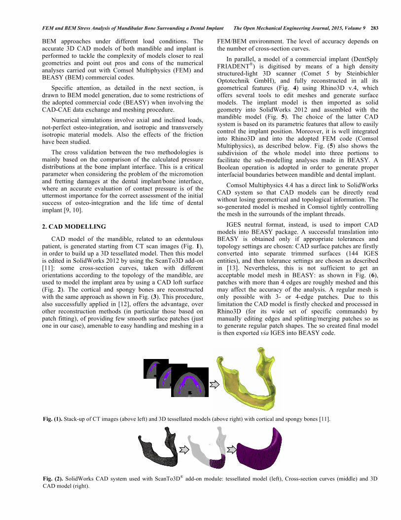
CAD model of the mandible, related to an edentulous patient, is generated starting from CT scan images (Fig. 1), in order to build up a 3D tessellated model. Then this model is edited in SolidWorks 2012 by using the ScanTo3D add-on [11]: some cross-section curves, taken with different orientations according to the topology of the mandible, are used to model the implant area by using a CAD loft surface (Fig. 2). The cortical and spongy bones are reconstructed with the same approach as shown in Fig. (3). This procedure, also successfully applied in [12], offers the advantage, over other reconstruction methods (in particular those based on patch fitting), of providing few smooth surface patches (just one in our case), amenable to easy handling and meshing in a

FEM/BEM environment. The level of accuracy depends on the number of cross-section curves. In parallel, a model of a commercial implant (DentSply FRIADENT®) is digitised by means of a high density structured-light 3D scanner (Comet 5 by Steinbichler Optotechnik GmbH), and fully reconstructed in all its geometrical features (Fig. 4) using Rhino3D v.4, which offers several tools to edit meshes and generate surface models. The implant model is then imported as solid geometry into SolidWorks 2012 and assembled with the mandible model (Fig. 5). The choice of the latter CAD system is based on its parametric features that allow to easily control the implant position. Moreover, it is well integrated into Rhino3D and into the adopted FEM code (Comsol Multiphysics), as described below. Fig. (5) also shows the subdivision of the whole model into three portions to facilitate the sub-modelling analyses made in BEASY. A Boolean operation is adopted in order to generate proper interfacial boundaries between mandible and dental implant. Comsol Multiphysics 4.4 has a direct link to SolidWorks CAD system so that CAD models can be directly read without losing geometrical and topological information. The so-generated model is meshed in Comsol tightly controlling the mesh in the surrounds of the implant threads. IGES neutral format, instead, is used to import CAD models into BEASY package. A successful translation into BEASY is obtained only if appropriate tolerances and topology settings are chosen: CAD surface patches are firstly converted into separate trimmed surfaces (144 IGES entities), and then tolerance settings are chosen as described in [13]. Nevertheless, this is not sufficient to get an acceptable model mesh in BEASY: as shown in Fig. (6), patches with more than 4 edges are roughly meshed and this may affect the accuracy of the analysis. A regular mesh is only possible with 3- or 4-edge patches. Due to this limitation the CAD model is firstly checked and processed in Rhino3D (for its wide set of specific commands) by manually editing edges and splitting/merging patches so as to generate regular patch shapes. The so created final model is then exported via IGES into BEASY code.

Fig. (1). Stack-up of CT images (above left) and 3D tessellated models (above right) with cortical and spongy bones [11].

Fig. (2). SolidWorks CAD system used with ScanTo3D® add-on module: tessellated model (left), Cross-section curves (middle) and 3D CAD model (right).

284 The Open Mechanical Engineering Journal, 2015, Volume 9 Perrella et al.

Fig. (3). CAD model of the mandible with highlight of cortical and spongy bone.

Fig. (4). 3D implant model: overall length 17.7 mm, thread diameter 3.75 mm, pitch 0.6 mm.

3. MATERIALS AND METHODS

Material properties greatly influence the stress-strain distribution in a bone-implant structure [5, 14]. If, on the one hand, for the implant a linear elastic and isotropic behaviour can be assumed (dental implants are usually made of Titanium alloys), on the other hand bone tissue is a more sophisticated structure, whose mechanical properties depend on several factors: age, gender, pathology, anatomical site, liquid content and so on [15]. With respect to the maxillary-mandible site, several contributions pointed out the bone mechanical properties [16]. Many of these contributions assumed both cortical and spongy bones as linear and isotropic. As demonstrated also in [17], this assumption corresponds to the approximation of a type II bone density. Other contributions, instead, considered a more realistic anisotropic law [2-6], also trying to capture the change of bone density in all space directions. A review of the available literature on computational modelling in the area of bone biomechanics, fracture and healing is available in [18]. Since the aim of the present research is to compare numerical results coming from FEM and BEM numerical

approaches, pointing out advantages and drawbacks in terms of stress-strain accuracy, both cases of isotropic and transversely isotropic (Fig. 7) behaviour for both cortical and spongy bones are considered. Tables 1 and 2 report the adopted isotropic and transversely isotropic material mechanical properties, respectively. Mastication involves repeated cyclic forces that are transferred to the bone tissue by the implant. Literature shows that mastication loads can significantly vary from one area of the mouth to another. As reported in [15], average forces of nearly 800 N for male young adults and 600 N for female young adults have been recorded in the molar region. In the premolar region, occlusal forces range from 200 to 600 N. Forces lower than 200 N have been measured in the incisal region. Such a variation may be related to many factors, such as muscle size, bone shape, gender, age, degree of edentulism. In the present paper, we work with an endosseous implant located in the premolar-incisal regions. The occlusal load is assumed equal to 350 N, statically applied on the upper surface of the implant and acting along its longitudinal axis or with a given inclination (α1=16°), configuring in such a way an added lateral mastication force (Fig. 7). Only half of the original reconstructed mandible is considered for numerical analyses, clamped on the two cutting surfaces as shown in Fig. (8). In all the analyses contacts are introduced at the interface between implant and cortical bone (Fig. 9), with and without friction as detailed in the following. Where friction is applied it is assumed µ=0.42. Table 3 summarises the five alternatives hypotheses adopted in the numerical FEM and BEM analyses. The compenetration between implant and cortical bone at the ring “planar supporting” area (Fig. 10) can be allowed, using internal spring of negligible stiffness (Hyp. 2 to 5), or not allowed using contact pairs (Hyp. 1). The former configures a more realistic condition in which the occlusal load is mainly absorbed at the implant thread level rather than in a very restricted area: the ring “planar supporting” area would absorb nearly 60% of the applied load if compenetration is not allowed. Moreover, the sliding between implant and bone is modelled with or without friction (Hyp. 2 to 5): where applied, the friction coefficient µ is set to 0.42 [2].

Fig. (5). Final CAD model being processed.

Final CAD modelImplant model Bone model


Fig. (6). Detail of the distorted mesh originally generated in BEASY due to the multi-edge patches coming from the CAD model.

4. FE MODEL

As previously mentioned, the CAD model shown in Fig. (8) is exported from SolidWorks to Comsol by using the LiveLink connection by Comsol. In the FEM environment the tetrahedral mesh is generated (Fig. 11) with a high refinement with linear elements in the middle portion of the model around the implant area and, in particular, along the

threaded region between the dental implant and the cortical bone, in order to obtain an accurate analysis in the contact zone. The final model consists of about 730’000 degrees of freedom (dofs). Table 1. Isotropic material properties (E: Young Modulus, ν:

Poisson ratio) [15, 19].

Implant Cortical Bone Spongy Bone

E [GPa] 120.0 13.7 1.37

ν 0.33 0.30 0.30

Numerical simulations are performed by considering a not-perfect osteo-integration. This is modelled by defining contact pairs at the implant-cortical interface. We assume that the implant has a lack of integration just in

correspondence of those threads interacting with the cortical bone, where the stress reach the highest values. Thus, the implant-spongy interface is modelled with a node-to-node identity so having a congruent mesh within Comsol. The choice of linear elements is done in order to reduce the number of dofs and to speed up the solution convergence.

Fig. (7). Different views of the analysed mandible portion: (x*-z*) is the local isotropic plane whereas xyz is the global coordinate system.

Fig. (8). Global model and sub-model (central dark coloured volume).

α1=16°

α2=45.2°

x

z x

y

sub-model full-model

cutting boundary

clamped boundary

clamped boundary

cutting boundary

quadratic domain (BEM)

quadratic domain (BEM)


Table 2. Transversely isotropic properties [4].

Cortical Bone Spongy Bone

Ex [GPa] 13.600 0.346

Ey [GPa] 24.000 1.040

Ez [GPa] 13.600 0.346

νxy 0.236 0.236

νyz 0.236 0.236

νxz 0.345 0.345

Gxy [GPa] 4.800 0.208

Gyz [GPa] 4.800 0.208

Gyz [GPa] 5.060 0.129 The adopted implant is made of Ti 6Al-4V titanium alloy [19].

Fig. (9). Highlight of the interface area between implant and cortical bone where contacts are added.

5. BE MODEL

BE model (Fig. 12) is based on a mixed linear-quadratic mesh with 4’300 elements: the higher polynomial order is provided in correspondence of the interface between the

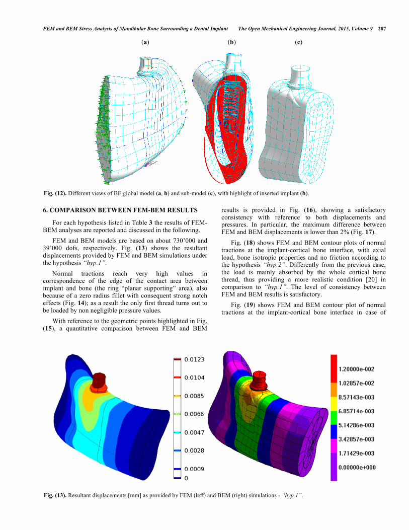
cortical bone and the implant, where highest stress gradients are expected. In the BEM environment we adopt the approach based on the extraction of a sub-model involving the volume surrounding the implant, i.e. the middle portion of the whole model (Fig. 12c).

Fig. (10). The occlusal load is mainly absorbed by the planar supporting provided by a very limited ring external cortical bone surface.

As for the FEM model, in case of not perfect osteo-integration between the implant and the cortical bone, the analysis becomes nonlinear with gap elements at the interface; for the remaining part of the implant, in contact with the spongy bone, a perfect osteo-integration is supposed and consequently the continuity is modelled for tractions and displacements. When considering a pure axial load, a mesh made of only linear elements (also in the critical area of implant/cortical bone interface) is sufficient to get accurate results, whereas, with an inclined load the use of quadratic elements in the critical areas is recommended.

“Planar Supporting”area

Fig. (11). FE mesh model and close-up of the threaded cortical region.

Table 3. Assumptions for FEM and BEM analyses.

Hypothesis Load type Bone Material Model Friction FEM Friction BEM “Planar Supporting”

1 Axial Isotropic No No Yes

2 Axial Isotropic No/Yes No/Yes No

3 Inclined Isotropic No/Yes No/Yes No

4 Axial Transversely isotropic No/Yes No/Yes No

5 Inclined Transversely isotropic No/Yes No/Yes No


6. COMPARISON BETWEEN FEM-BEM RESULTS

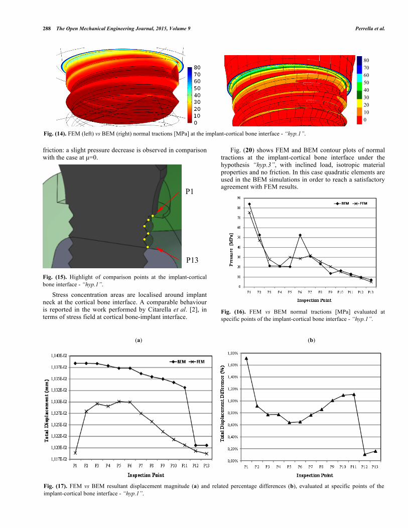
For each hypothesis listed in Table 3 the results of FEM-BEM analyses are reported and discussed in the following. FEM and BEM models are based on about 730’000 and 39’000 dofs, respectively. Fig. (13) shows the resultant displacements provided by FEM and BEM simulations under the hypothesis “hyp.1”. Normal tractions reach very high values in correspondence of the edge of the contact area between implant and bone (the ring “planar supporting” area), also because of a zero radius fillet with consequent strong notch effects (Fig. 14); as a result the only first thread turns out to be loaded by non negligible pressure values. With reference to the geometric points highlighted in Fig. (15), a quantitative comparison between FEM and BEM

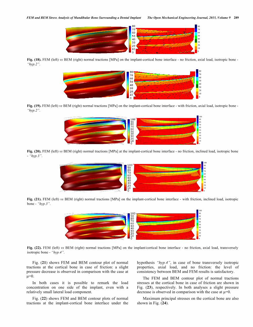
results is provided in Fig. (16), showing a satisfactory consistency with reference to both displacements and pressures. In particular, the maximum difference between FEM and BEM displacements is lower than 2% (Fig. 17). Fig. (18) shows FEM and BEM contour plots of normal tractions at the implant-cortical bone interface, with axial load, bone isotropic properties and no friction according to the hypothesis “hyp.2”. Differently from the previous case, the load is mainly absorbed by the whole cortical bone thread, thus providing a more realistic condition [20] in comparison to “hyp.1”. The level of consistency between FEM and BEM results is satisfactory. Fig. (19) shows FEM and BEM contour plot of normal tractions at the implant-cortical bone interface in case of

(a) (b) (c)

Fig. (12). Different views of BE global model (a, b) and sub-model (c), with highlight of inserted implant (b).

Fig. (13). Resultant displacements [mm] as provided by FEM (left) and BEM (right) simulations - “hyp.1”.


friction: a slight pressure decrease is observed in comparison with the case at µ=0.

Fig. (15). Highlight of comparison points at the implant-cortical bone interface - “hyp.1”.

Stress concentration areas are localised around implant neck at the cortical bone interface. A comparable behaviour is reported in the work performed by Citarella et al. [2], in terms of stress field at cortical bone-implant interface.

Fig. (20) shows FEM and BEM contour plots of normal tractions at the implant-cortical bone interface under the hypothesis “hyp.3”, with inclined load, isotropic material properties and no friction. In this case quadratic elements are used in the BEM simulations in order to reach a satisfactory agreement with FEM results.

Fig. (16). FEM vs BEM normal tractions [MPa] evaluated at specific points of the implant-cortical bone interface - “hyp.1”.

P1

P13

Fig. (14). FEM (left) vs BEM (right) normal tractions [MPa] at the implant-cortical bone interface - “hyp.1”.

(a) (b)

Fig. (17). FEM vs BEM resultant displacement magnitude (a) and related percentage differences (b), evaluated at specific points of the implant-cortical bone interface - “hyp.1”.

80 70 60 50 40 30 20 10 0


Fig. (21) shows FEM and BEM contour plot of normal tractions at the cortical bone in case of friction: a slight pressure decrease is observed in comparison with the case at µ=0. In both cases it is possible to remark the load concentration on one side of the implant, even with a relatively small lateral load component. Fig. (22) shows FEM and BEM contour plots of normal tractions at the implant-cortical bone interface under the

hypothesis “hyp.4”, in case of bone transversely isotropic properties, axial load, and no friction: the level of consistency between BEM and FEM results is satisfactory. The FEM and BEM contour plot of normal tractions stresses at the cortical bone in case of friction are shown in Fig. (23), respectively. In both analyses a slight pressure decrease is observed in comparison with the case at µ=0. Maximum principal stresses on the cortical bone are also shown in Fig. (24).

Fig. (18). FEM (left) vs BEM (right) normal tractions [MPa] on the implant-cortical bone interface - no friction, axial load, isotropic bone - “hyp.2”.

Fig. (19). FEM (left) vs BEM (right) normal tractions [MPa] on the implant-cortical bone interface - with friction, axial load, isotropic bone - “hyp.2”.

Fig. (20). FEM (left) vs BEM (right) normal tractions [MPa] at the implant-cortical bone interface - no friction, inclined load, isotropic bone - “hyp.3”.

Fig. (21). FEM (left) vs BEM (right) normal tractions [MPa] on the implant-cortical bone interface - with friction, inclined load, isotropic bone - “hyp.3”.

Fig. (22). FEM (left) vs BEM (right) normal tractions [MPa] on the implant/cortical bone interface - no friction, axial load, transversely isotropic bone - “hyp.4”.

80 70 60 50 40 30 20 10 0

80 70 60 50 40 30 20 10 0

100 90 80 70 60 50 40 30 20 10 0

100 90 80 70 60 50 40 30 20 10 0

100 90 80 70 60 50 40 30 20 10 0


Moreover, the maximum principal stress fields obtained with the two methodologies are in good agreement, highlighting a critical area in the upper part of the cortical shell. Fig. (25) shows the FEM and BEM contour plots of normal tractions at the implant-cortical bone interface, in case of transversely isotropic properties and inclined load according to the hypothesis “hyp.5”. Again, quadratic elements are necessary in the BEM simulations in order to get a satisfactory consistency with FEM results. The comparisons of the contour plots of normal tractions and maximum principal stresses at the cortical bone in case of friction are depicted in Figs. (26, 27), respectively, displaying, as in the previous cases, a sound agreement.

CONCLUSION

This paper shows a cross comparison between two numerical methodologies (FEM and BEM) as implemented

in two different commercial codes applied to a bio-mechanical problem. Different conditions are adopted to handle dental implant issues such as the isotropic and transversely isotropic material behaviour for cortical and spongy bones as well as the presence or absence of friction on the interface between implant and cortical bone. Moreover, the modelled complex geometries are very close to the real ones as accurate reconstruction techniques are used. Numerical results demonstrate an overall good agreement between the two methodologies even though they are related to the specific software adopted in the simulations: Comsol Multiphysics for FEM and BEASY for BEM. With respect to these codes some remarks can be outlined from this study. The CAD-CAE integration level is very high in Comsol environment as a direct link with common CAD software is available and well tested for several native and neutral formats of data exchange. Thus, complex geometric models can be successfully imported and, in case of data exchange

Fig. (23). FEM (left) vs BEM (right) normal tractions [MPa] on the implant/cortical bone interface - with friction, axial load, transversely isotropic bone - “hyp.4”.

Fig. (24). FEM (left) vs BEM (right) maximum principal stresses on the cortical bone [MPa] - with friction, axial load, transversely isotropic bone - “hyp.4”.

Fig. (25). FEM (left) vs BEM (right) normal tractions [MPa] on the implant/cortical bone interface - no friction, inclined load, transversely isotropic bone - “hyp.5”.

Fig. (26). FEM (left) vs BEM (right) normal tractions [MPa] on the implant/cortical bone interface - with friction, inclined load, transversely isotropic bone - “hyp.5”.

110 100 90 80 70 60 50 40 30 20 10 0

75 60 46 31 17 2.2 -12 -27 -41 -56 -70 -85

100 90 80 70 60 50 40 30 20 10 0

100 90 80 70 60 50 40 30 20 10 0


problems, healing tools are available to repair the model. The internal automatic mesher performs satisfactorily with little user intervention. Nevertheless, a very dense mesh is required to get good results, especially in case of nonlinear contact analysis without or with friction. In the latter case, in the previous versions of the Comsol software it was necessary appropriately setting the internal parameters for the penalty factor, while with the used version 4.4 it is just enough to adopt the suggested preset parameters and the solution converges. On the other hand, using BEASY code, it is difficult to handle complex geometries and particular attention must be devoted to the right settings of the parameters controlling the translation of native CAD geometries. Moreover, very few repairing tools are available to heal topology issues, so that a trial and error approach is often necessary. To obtain a good quality mesh the model topology must be controlled at a CAD level: an accurate tailored modelling task is necessary to generate in the CAD environment the single patches with only 3- or 4-edges. For this task Rhino3D is used: it provides several specific and powerful editing tools, not available in many other CAD environments. This is a very time-consuming task. Nevertheless, when facing non-linear simulations, involving contact pairs, BEM approach gives results comparable with those obtained with FEM on the boundary pairs, without drastically reducing the mean mesh size. On the contrary, the FEM solution is quite sensitive to the local mesh size around the contact pairs: to improve the accuracy, a very fine local mesh is required. The comparison between the two models is judged acceptable, although it is the authors' opinion that for a complete validation further analyses should be carried on.

CONFLICT OF INTEREST

The authors confirm that this article content has no conflict of interest.

ACKNOWLEDGEMENTS

Declared none.

REFERENCES

[1] E. Kitamura, R. Stegaroiu, S. Nomura, and O. Miyakawa, “Biomechanical aspects of marginal bone resorption around osseointegrated implants: considerations based on a three–dimensional finite element analysis”, Clin. Oral Implant. Res., vol. 15, no. 4, pp. 401-412, 2004.

[2] R. Citarella, E. Armentani, F. Caputo, and M. Lepore, “Stress analysis of an endosseus dental implant by BEM and FEM”, Open

Mech. Eng. J., vol. 6, pp. 115-124, 2012. DOI: 10.2174/1874155X01206010115.

[3] E. Armentani, F. Caputo, and R. Citarella, “FEM sensitivity analyses on the stress levels in a human mandible with a varying ATM modelling complexity”, Open Mech. Eng. J., vol. 4, pp. 8-15, 2010. DOI: 10.2174/1874155X01004010008.

[4] R. Citarella, E. Armentani, F. Caputo, and A. Naddeo, “FEM and BEM analysis of a human mandible with added temporomandibular joints”, Open Mech. Eng. J., vol. 6, pp. 100-114, 2012. DOI: 10.2174/1874155X01206010100.

[5] G. Sammartino, G. Marenzi, R. Citarella, R. Ciccarelli, and H-L. Wang, “Analysis of the occlusal stress transmitted to the inferior alveolar nerve by an osseointegrated threaded fixture”, J. Periodontol., vol. 79, no. 9, pp. 1735-1744, 2008, DOI: 10.1902/ jop.2008.080030.

[6] G. Sammartino, Hom-Lay Wang, R. Citarella, M. Lepore, and G. Marenzi, “Analysis of occlusal stresses transmitted to the inferior alveolar nerve by multiple threaded implants”, J. Periodontol., vol. 84, no. 11, pp. 1655-1661, 2013. DOI: 10.1902/jop.2013. 120611.

[7] P. Franciosa, M. Martorelli, “Stress-based performance comparison of dental implants by finite element analysis”, Int. J. Interact. Des. Manuf., vol. 6, pp. 123-129, 2012. DOI 10.1007/s12008-012-0155-y

[8] P. Ausiello, P. Franciosa, M. Martorelli, and D.C. Watts, “Effects of thread features in osseo-integrated titanium implants using a statistics-based finite element method”, Dent. Mat., 2012. http://dx.doi.org/10.1016/j.dental.2012.04.035

[9] S.S. Gao, Y.R. Zhang, Z.L. Zhu, H.Y. Yu, “Micromotions and combined damages at the dental implant/bone interface”, Int. J. Oral Sci., vol. 4, no. 4, pp. 182-188, 2012. DOI: 10.1038/ijos.2012. 68.

[10] N. Murakami, N. Wakabayashi, “Finite element contact analysis as a critical technique in dental biomechanics: A review”, J. Prosthodont. Res., vol. 58, no. 2, pp. 92-101, 2014.

[11] S. Gerbino, and M. Martorelli, “Developing CAD procedures for automatic geometric reconstruction of a human mandible”, In Proc. Int Joint Congress XVII Ingegraf - XV ADM, Siviglia, Spain, Jun 2005.

[12] P. Ausiello, P. Franciosa, M. Martorelli, and D.C. Watts, “Mechanical behavior of post-restored upper canine teeth: A 3D FE analysis”, Dent. Mater., vol. 27, no. 12, pp. 1285-1294, 2011. DOI: http://dx.doi.org/10.1016/j.dental.2011.09.009

[13] R. Citarella, and S. Gerbino, “BE analysis of shuft-hub couplings with polygonal profiles”, J. Mater. Process. Technol., vol. 109, pp. 30-37, 2001.

[14] A. Natali, N.,and P.G. Pavan, “A comparative analysis based on different strength criteria for evaluation of risk factor for dental implants”, Comput. Methods Biomech. Biomed. Eng., vol. 5, pp. 127-133, 2002.

[15] Ming-Lun Hsu, and Chih-Ling Chang, “Application of Finite Element Analysis in Dentistry”, InTech, In: D. Moratal, Ed. 2010.

[16] J.M. Reina, J.M. Garcia-Aznar, J. Dominguez, and M. Doblarè, “Numerical estimation of bone density and elastic constants distribution in a human mandible”, J. Biomech., vol. 40, no. 4, pp. 828-836, 2007.

[17] L. Baggi, I. Cappelloni, M. Di Girolamo, F. Maceri, and G. Vairo, “The influence of implant diameter and length on stress distribution of osseointegrated implants related to crestal bone geometry: A three dimensional finite element analysis”, J. Prosthet. Dent., vol. 100, pp. 422-431, 2008.

Fig. (27). FEM (left) vs BEM (right) maximum principal stresses on the cortical bone [MPa] - with friction, inclined load, transversely isotropic bone - “hyp.5”.

75 60 46 31 17 2.2 -12 -27 -41 -56 -70 -85


[18] M. Doblarè, J.M. Garcia, and M.J. Gomez, “Modelling bone tissue fracture and healing: a review”, Eng. Fract. Mech., vol. 71, pp. 1809-1840, 2004.

[19] http://www.arcam.com/wp-content/uploads/Arcam-Ti6Al4V-Titan-ium-Alloy.pdf [Accessed: Dec 19th 2014].

[20] W. Winter, D. Klein, M. Karl, “Micromotion of dental implants: basic mechanical considerations”, J. Med. Eng., vol. 2013, article ID 265412, pp. 1-9, 2013.

Received: January 8, 2015 Revised: January 15, 2015 Accepted: January 16, 2015 © Perrella et al.; Licensee Bentham Open.

This is an open access article licensed under the terms of the Creative Commons Attribution Non-Commercial License (http://creativecommons.org/licenses/by-nc/3.0/) which permits unrestricted, non-commercial use, distribution and reproduction in any medium, provided the work is properly cited.

282 The Open Mechanical Engineering Journal, Open Access ... · 3University of Molise, Engineering...

Documents

Transcript of 282 The Open Mechanical Engineering Journal, Open Access ... · 3University of Molise, Engineering...