28 - 1

CHAPTER 28Advanced Issues in Cash Management

and Inventory Control

Setting the target cash balanceEOQ modelBaumol Model

28 - 2

Theoretical models such as the Baumol model have been developed for use in setting target cash balances. The Baumol model is similar to the EOQ model, which will be discussed later.

Today, companies strive for zero cash balances and use borrowings or marketable securities as a reserve.

Monte Carlo simulation can be helpful in setting the target cash balance.

Setting the Target Cash Balance

28 - 3

Insufficient inventories can lead to lost sales.

Excess inventories means higher costs than necessary.

Large inventories, but wrong items leads to both high costs and lost sales.

Inventory management is more closely related to operations than to finance.

Why is inventory management vital to the financial health of most firms?

28 - 4

All values are known with certainty and constant over time.

Inventory usage is uniform over time.Carrying costs change proportionally with

changes in inventory levels.All ordering costs are fixed.These assumptions do not hold in the “real

world,” so safety stocks are held.

Assumptions of the EOQ Model

28 - 5

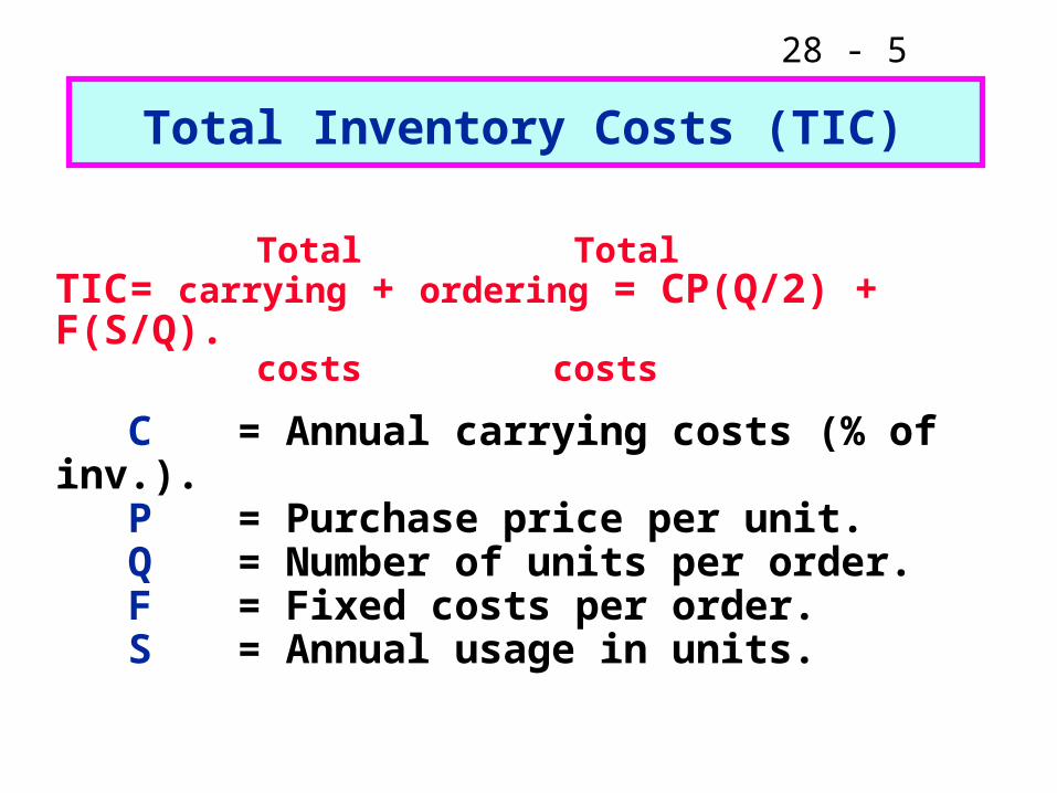
Total TotalTIC = carrying + ordering = CP(Q/2) + F(S/Q).

costs costs

C = Annual carrying costs (% of inv.). P = Purchase price per unit. Q = Number of units per order. F = Fixed costs per order. S = Annual usage in units.

Total Inventory Costs (TIC)

28 - 6

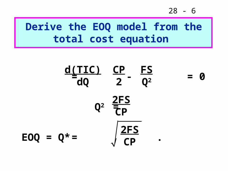
Derive the EOQ model from the total cost equation

= - = 0

Q2 =

EOQ = Q* = .2FSCP

d(TIC)dQ

CP2

FSQ2

2FSCP

28 - 7

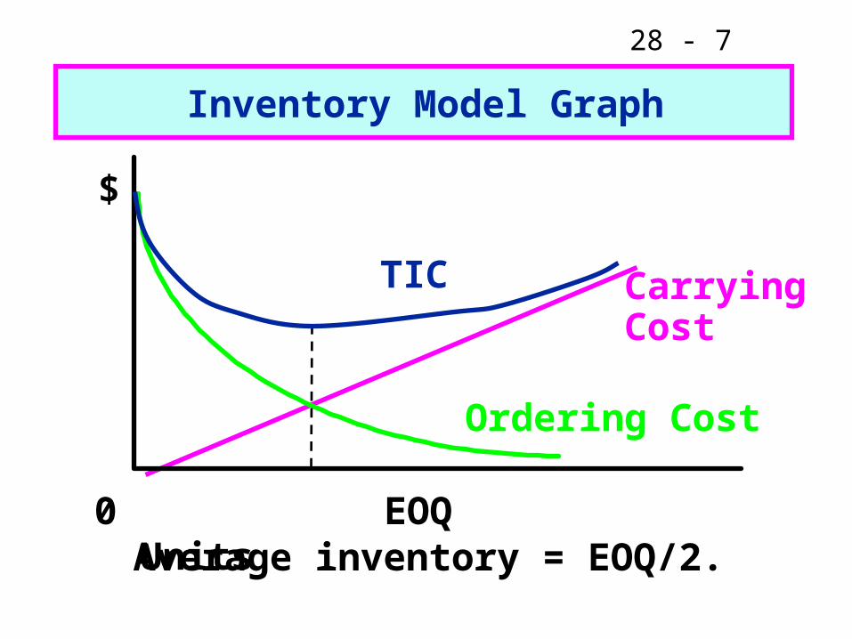
Inventory Model Graph

TIC Carrying Cost

Ordering Cost

0 EOQ Units

$

Average inventory = EOQ/2.

28 - 8

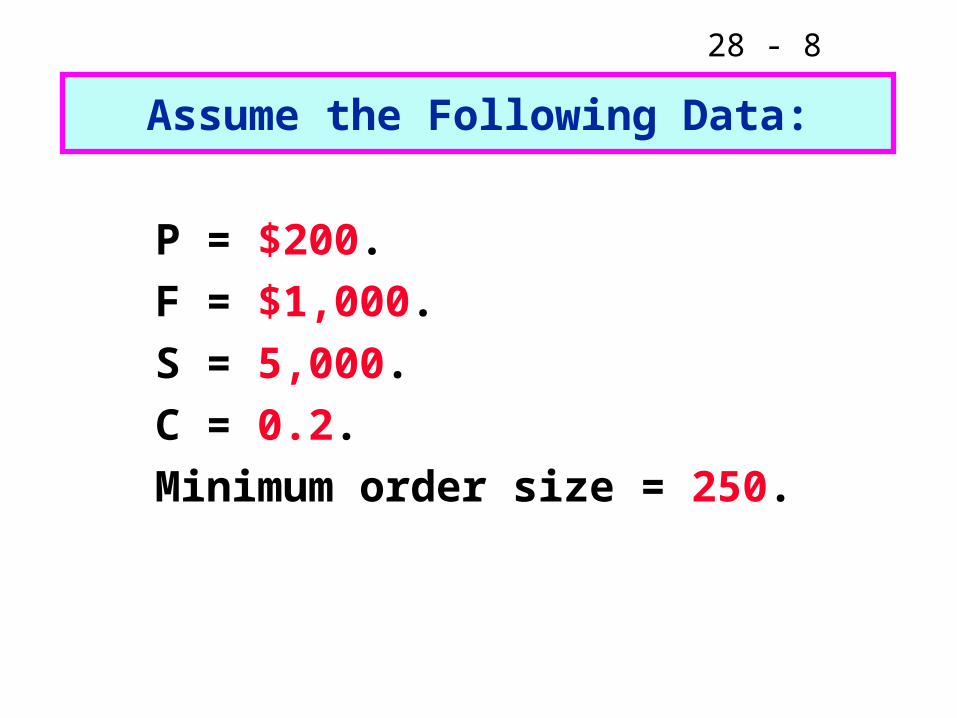
Assume the Following Data:

P = $200.

F = $1,000.

S = 5,000.

C = 0.2.

Minimum order size = 250.

28 - 9

What is the EOQ?

EOQ =

=

= 250,000 = 500 units.

2($1,000)(5,000)0.2($200)

$10,000,00040

28 - 10

TIC = CP( )+ F( )= (0.2)($200)(500/2) + $1,000(5,000/500)

= $40(250) + $1,000(10)

= $10,000 + $10,000 = $20,000.

What are total inventory costs when the EOQ is ordered?

Q2

SQ

28 - 11

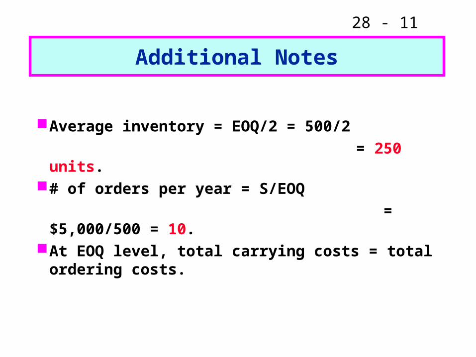
Additional Notes

Average inventory = EOQ/2 = 500/2

= 250 units.# of orders per year = S/EOQ

= $5,000/500 = 10.At EOQ level, total carrying costs = total

ordering costs.

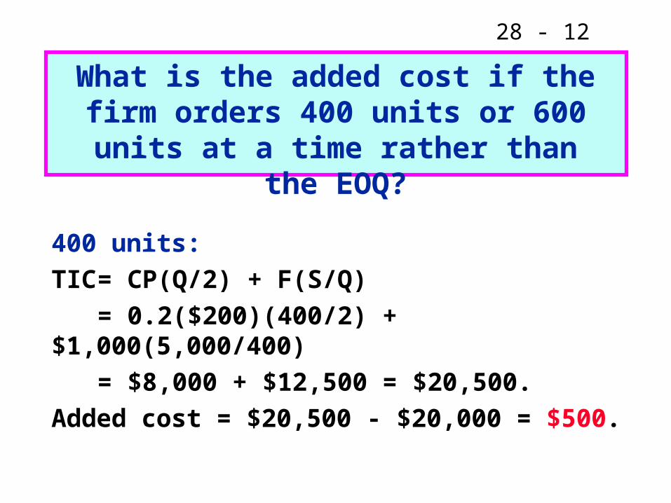
28 - 12

400 units:

TIC = CP(Q/2) + F(S/Q)

= 0.2($200)(400/2) + $1,000(5,000/400)

= $8,000 + $12,500 = $20,500.

Added cost = $20,500 - $20,000 = $500.

What is the added cost if the firm orders 400 units or 600 units at a time

rather than the EOQ?

28 - 13

600 units:

TIC = CP(Q/2) + F(S/Q)

= 0.2($200)(600/2) + $1,000(5,000/600)

= $12,000 +$8,333 = $20,333.

Added cost = $20,333 - $20,000 = $333.

28 - 14

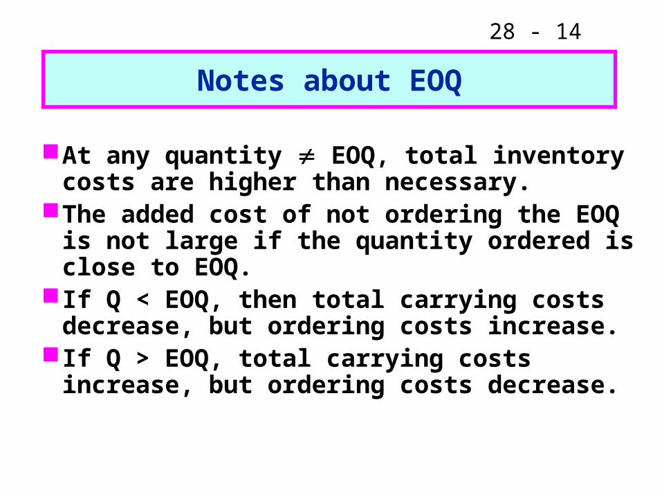
At any quantity EOQ, total inventory costs are higher than necessary.

The added cost of not ordering the EOQ is not large if the quantity ordered is close to EOQ.

If Q < EOQ, then total carrying costs decrease, but ordering costs increase.

If Q > EOQ, total carrying costs increase, but ordering costs decrease.

Notes about EOQ

28 - 15

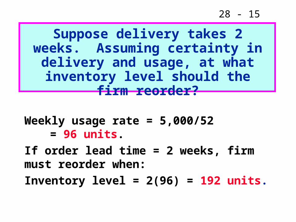
Weekly usage rate = 5,000/52 = 96 units.

If order lead time = 2 weeks, firm must reorder when:

Inventory level = 2(96) = 192 units.

Suppose delivery takes 2 weeks. Assuming certainty in delivery and

usage, at what inventory level should the firm reorder?

28 - 16

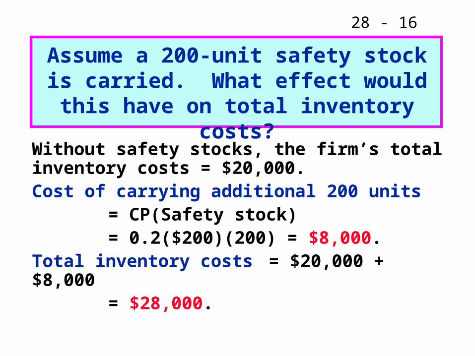
Without safety stocks, the firm’s total inventory costs = $20,000.Cost of carrying additional 200 units

= CP(Safety stock)= 0.2($200)(200) = $8,000.

Total inventory costs = $20,000 + $8,000= $28,000.

Assume a 200-unit safety stock is carried. What effect would this have

on total inventory costs?

28 - 17

Alternatively:

Average inventory = (500/2) + 200

= 450 units.

TIC = CP(Avg. Inv.) + F(S/Q)

= 0.2($200)(450) + $1,000(5,000/500)

= $18,000 + $10,000

= $28,000.

28 - 18

Reorder point = 200 + 192 = 392 units.The firm’s normal 96 unit usage

could rise to 392/2 = 196 units per week.

Or the firm could operate for 392/96 = 4 weeks while awaiting delivery of an order.

What is the new reorder point with the safety stock?

28 - 19

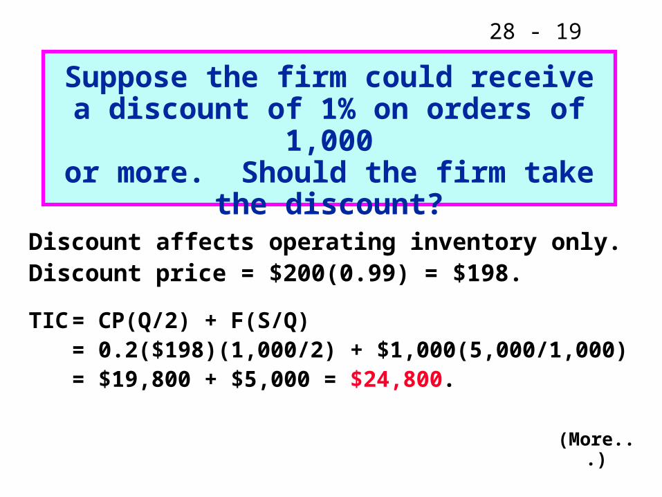
Discount affects operating inventory only.Discount price = $200(0.99) = $198.

TIC = CP(Q/2) + F(S/Q)= 0.2($198)(1,000/2) + $1,000(5,000/1,000)= $19,800 + $5,000 = $24,800.

Suppose the firm could receive a discount of 1% on orders of 1,000or more. Should the firm take the

discount?

(More...)

28 - 20

Savings = 0.01($200)(5,000) = $10,000

Added costs = $24,800 - $20,000 = $ 4,800

Net savings = $10,000 - $4,800 = $ 5,200

Firm should take the discount.

28 - 21

Yes, but it must be applied to shorter periods during which usage is approximately constant.

Can the EOQ be used if there are seasonal variations?

28 - 22

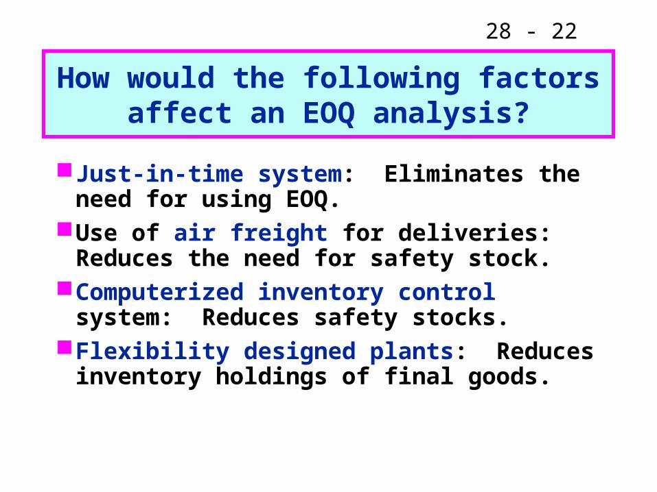
How would the following factors affect an EOQ analysis?

Just-in-time system: Eliminates the need for using EOQ.

Use of air freight for deliveries: Reduces the need for safety stock.

Computerized inventory control system: Reduces safety stocks.

Flexibility designed plants: Reduces inventory holdings of final goods.

28 - 23

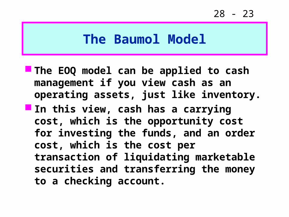
The Baumol Model

The EOQ model can be applied to cash management if you view cash as an operating assets, just like inventory.

In this view, cash has a carrying cost, which is the opportunity cost for investing the funds, and an order cost, which is the cost per transaction of liquidating marketable securities and transferring the money to a checking account.

28 - 24

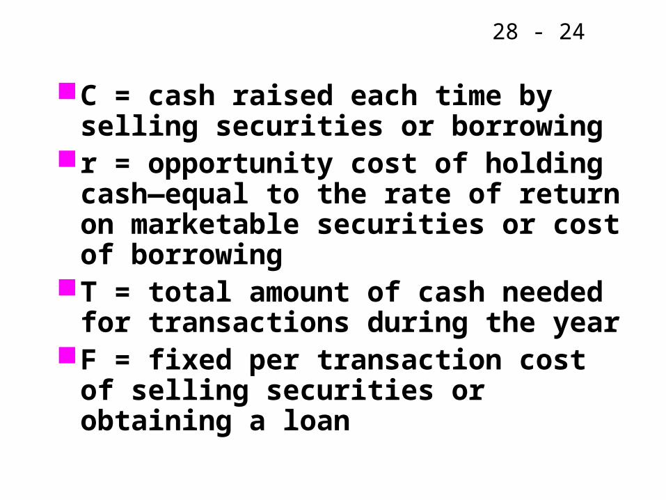
C = cash raised each time by selling securities or borrowing

r = opportunity cost of holding cash—equal to the rate of return on marketable securities or cost of borrowing

T = total amount of cash needed for transactions during the year

F = fixed per transaction cost of selling securities or obtaining a loan

28 - 25

Costs of cash—Holding costs

Holding cost

= (average cash balance)

x (opportunity cost rate)

Average cash balance = C/2

Holding cost = C/2 x r = rC/2

28 - 26

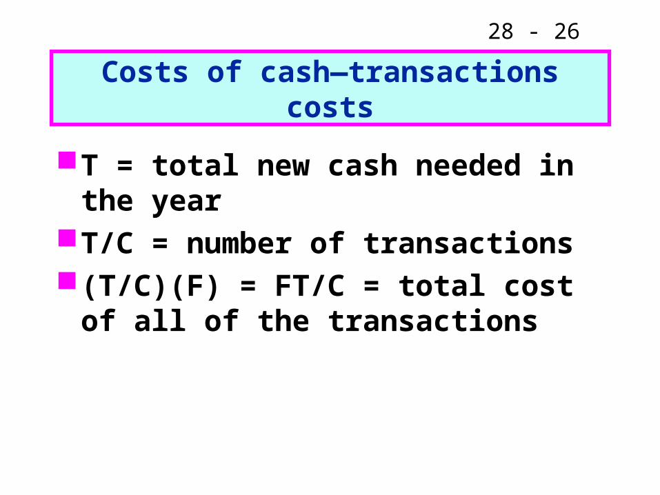
Costs of cash—transactions costs

T = total new cash needed in the yearT/C = number of transactions(T/C)(F) = FT/C = total cost of all of

the transactions

28 - 27

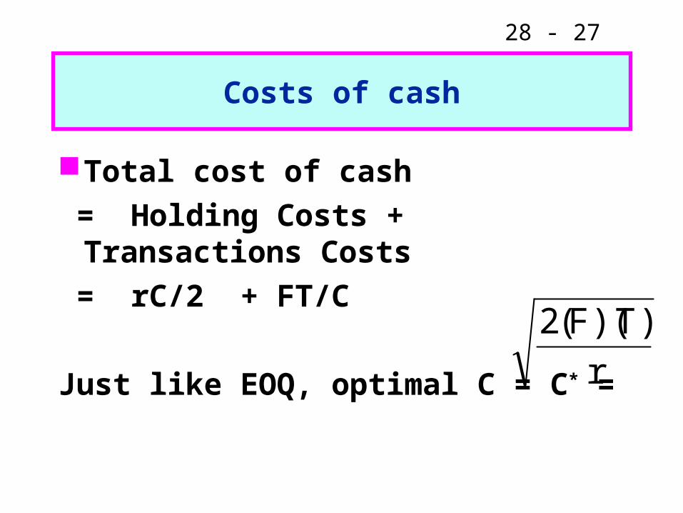
Costs of cash

Total cost of cash

= Holding Costs + Transactions Costs

= rC/2 + FT/C

Just like EOQ, optimal C = C* =r

)T)(F(2

28 - 28

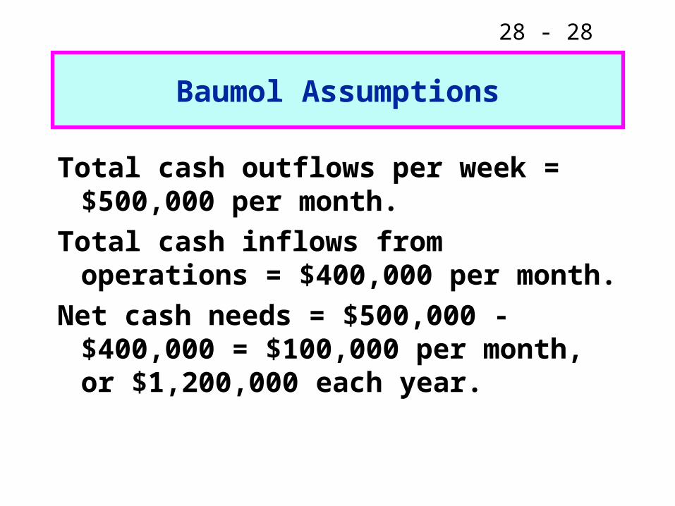
Baumol Assumptions

Total cash outflows per week = $500,000 per month.

Total cash inflows from operations = $400,000 per month.

Net cash needs = $500,000 - $400,000 = $100,000 per month, or $1,200,000 each year.

28 - 29

Costs:

Transaction/order costs = $32 per transaction (F)

r = 7% = rate the firm can earn on its marketable securities

123,33$07.0

)1200000)(32(2C*

28 - 30

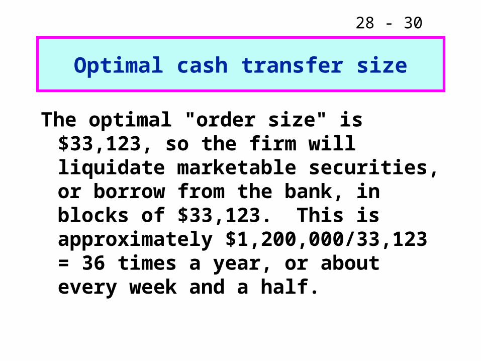
Optimal cash transfer size

The optimal "order size" is $33,123, so the firm will liquidate marketable securities, or borrow from the bank, in blocks of $33,123. This is approximately $1,200,000/33,123 = 36 times a year, or about every week and a half.

28 - 31

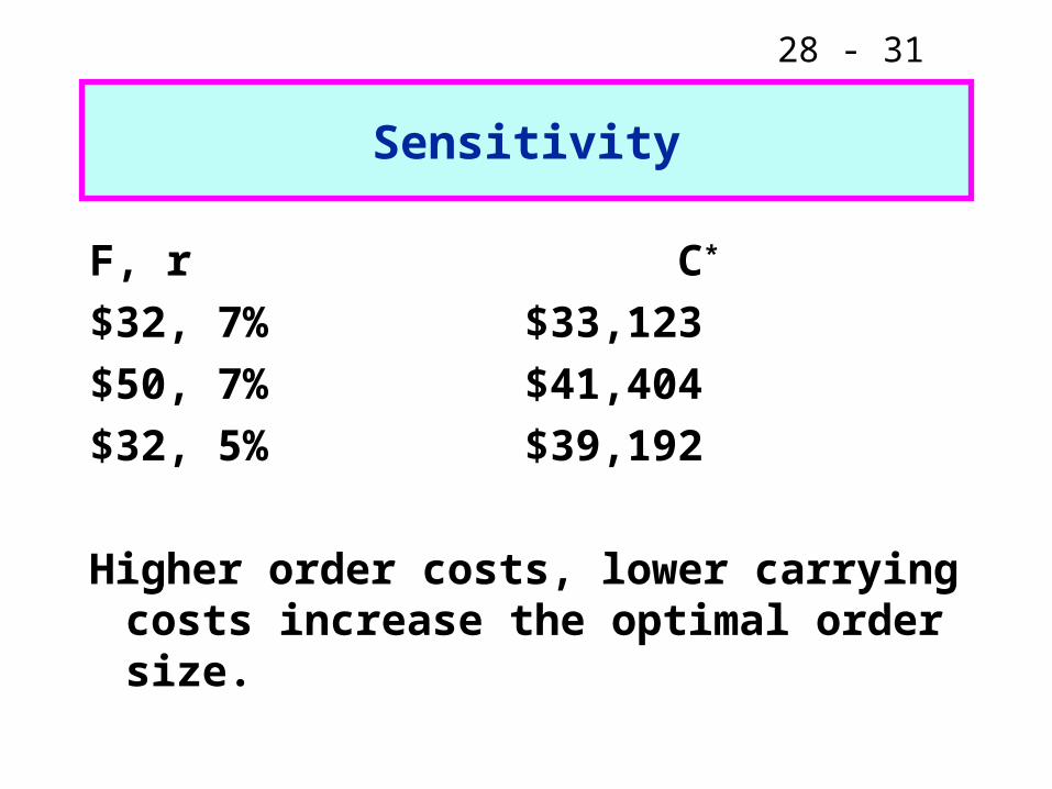
Sensitivity

F, r C*

$32, 7% $33,123

$50, 7% $41,404

$32, 5% $39,192

Higher order costs, lower carrying costs increase the optimal order size.